Closed cosmologies with a perfect fluid and a scalar field

Abstract

Closed, spatially homogeneous cosmological models with a perfect fluid and a scalar field with exponential potential are investigated, using dynamical systems methods. First, we consider the closed Friedmann-Robertson-Walker models, discussing the global dynamics in detail. Next, we investigate Kantowski-Sachs models, for which the future and past attractors are determined. The global asymptotic behaviour of both the Friedmann-Robertson-Walker and the Kantowski-Sachs models is that they either expand from an initial singularity, reach a maximum expansion and thereafter recollapse to a final singularity (for all values of the potential parameter $\kappa$), or else they expand forever towards a flat power-law inflationary solution (when $\kappa^{2}<2$). As an illustration of the intermediate dynamical behaviour of the Kantowski-Sachs models, we examine the cases of no barotropic fluid, and of a massless scalar field in detail. We also briefly discuss Bianchi type IX models.

I Introduction

Cosmological models with a scalar field and an exponential potential are of fundamental importance in the study of the universe. These models are motivated by the fact that they arise naturally in alternative theories of gravity and occur as the low-energy limit in supergravity theories [1, 2]. By using qualitative techniques, the well-known power-law inflationary solution has been shown to be an attractor for all initially expanding Bianchi models (except a subclass of the Bianchi type IX models which will recollapse) in the class of spatially homogeneous Bianchi models [3, 4]. More recently, cosmological models which contain both barotropic matter and a scalar field with an exponential potential have been studied [5], partially motivated by the fact that there exist spatially flat isotropic scaling solutions in which the energy density due to the scalar field is proportional to the energy density of the perfect fluid [6]. In [7] the stability of these cosmological scaling solutions within the class of spatially homogeneous cosmological models with a perfect fluid subject to the equation of state $p=(\gamma-1)\mu$ (where $\gamma$ is a constant satisfying $0<\gamma<2$) was studied and it was found that when $\gamma>2/3$, and particularly for realistic matter with $\gamma\geq 1$, the scaling solutions are unstable; essentially they are unstable to curvature perturbations, although they are stable to shear perturbations. In addition, in [8] homogeneous and isotropic spacetimes with non-zero spatial curvature were studied.

It is clearly of interest to study more general cosmological models. One class of models of particular interest are those with positive spatial curvature. These models have attracted less attention since they are more complicated mathematically. Positive-curvature Friedmann-Robertson-Walker (FRW) models [8, 9, 10, 11], Kantowski-Sachs models [12] and Bianchi type IX models [3, 10, 13, 14] have been studied using qualitative methods, although rigorous analyses using a new set of compact variables have not been carried out. The Bianchi type IX models are known to have very complicated dynamics, exhibiting the characteristics of chaos [10, 15], and are hence beyond the scope of the present study. Recently [16] positive-curvature FRW models and Kantowski-Sachs models with a perfect fluid and a cosmological constant have been investigated using qualitative methods and utilizing compactified variables.

The outline of this paper is as follows. We shall first comprehensively study the qualitative properties of the class of positive-curvature FRW models with a barotropic fluid and a non-interacting scalar field with an exponential potential, extending and generalising work by Turner [17], who used different basic variables. We shall then analyse the qualitative properties of the Kantowski-Sachs models. Positive-curvature FRW models and Kantowski-Sachs models belong to the class of spherically symmetric models, and hence the present work is a natural extension of recent work [18, 19]. Indeed, it turns out that understanding the dynamics of the Kantowski-Sachs models is crucial for understanding the global dynamics of general spherically symmetric similarity models [20].

A Matter model

The matter content of the models is taken to be a perfect fluid and a scalar field with exponential potential. The corresponding energy-momentum tensor is

$$T_{ab} = (T_{{\rm pf}\,ab}+T_{{\rm sf}\,ab}),$$ (1)

$$T_{{\rm pf}\,ab} = \mu u_{a}u_{b}+p\left(u_{a}u_{b}+g_{ab}\right),$$ (2)

$$T_{{\rm sf}\,ab} = \phi_{,a}\phi_{,b}-\left(\frac{1}{2}\phi_{,c}\phi^{,c}+V(\phi)\right)g_{ab},$$ (3)

$$V(\phi) = V_{0}e^{-\kappa\phi},$$ (4)

where $\kappa$ is a non-negative constant, and the pressure is given by $p=(\gamma-1)\mu$, with the equation-of-state parameter in the range $1\leq\gamma\leq 2$. The fluid energy density $\mu$ and the scalar field $\phi$ are functions of a timelike coordinate $t$. A dot denotes differentiation with respect to $t$ and throughout units are used in which $c=8\pi G=1$. The matter components are assumed to be non-coupled, and thus they are separately conserved:

$$\nabla_{a}T_{\rm pf}^{ab}= 0 =\nabla_{a}T_{\rm sf}^{ab}.$$ (5)

For convenience, we define

$$X=\frac{1}{\sqrt{2}}\dot{\phi}.$$ (6)

II Closed Friedmann models

We start our investigation of closed cosmological models with a perfect fluid and a scalar field by looking at the closed FRW models. The line element for these models can be written

$$ds^{2}=-dt^{2}+S(t)^{2}dr^{2}+S(t)^{2}\sin^{2}r\,d\Omega^{2}.$$ (7)

The expansion of the fluid congruence is given by $\theta=3\dot{S}/S$, and the evolution equation for the curvature $K\equiv 9/(\theta^{2}S^{2})$ is

$$\dot{K}=-\frac{2K}{3\theta}(3\dot{\theta}+\theta^{2}).$$ (8)

The conservation equations yield

$$\dot{\mu} = -\gamma\theta\mu,$$ (9)

$$\dot{X} = -\theta X+\frac{\kappa}{\sqrt{2}}V.$$ (10)

From the field equations we obtain

$$\mu = \frac{1}{3}\left[(1+K)\theta^{2}-3X^{2}-3V\right],$$ (11)

$$\dot{\theta} = -\frac{1}{3}\left\{\theta^{2}+\frac{1}{2}D^{2}+\frac{3}{2}\left[3X^{2}-3V+3(\gamma-1)\mu\right]\right\}.$$ (12)

Assuming $\mu\geq 0$, the Friedmann equation, Eq. (11), shows that $D=\sqrt{(1+K)\theta^{2}}$ is a dominant quantity. Thus, compact variables can be defined according to

$$Q_{0}=\frac{\theta}{D},\quad U=\frac{\sqrt{3}X}{D},\quad W=\frac{\sqrt{3V}}{D}.$$ (13)

Note also that the curvature is given by

$$K=\frac{1-Q_{0}^{2}}{Q_{0}^{2}}.$$ (14)

The Friedmann equation becomes

$$\Omega_{D}=\frac{3\mu}{D^{2}}=1-U^{2}-W^{2}.$$ (15)

Defining a new independent variable, ${}^{\prime}=d/d\tau=\frac{3}{D}\,d/dt$, the evolution equation for $D$

$$D^{\prime} = -3Q_{0}\left(U^{2}+\frac{\gamma}{2}\Omega_{D}\right)D$$ (16)

decouples. Thus, a reduced set of evolution equations is obtained:

$$Q_{0}^{\prime} = (1-Q_{0}^{2})\left[1-3\left(U^{2}+\frac{\gamma}{2}\Omega_{D}\right)\right],$$ (17)

$$U^{\prime} = 3Q_{0}U\left[-1+\left(U^{2}+\frac{\gamma}{2}\Omega_{D}\right)\right]+\sqrt{\frac{3}{2}}\kappa W^{2},$$ (18)

$$W^{\prime} = 3Q_{0}\left(U^{2}+\frac{\gamma}{2}\Omega_{D}\right)W-\sqrt{\frac{3}{2}}\kappa UW.$$ (19)

There is also an auxiliary evolution equation

$$\Omega_{D}^{\prime}=-3Q_{0}\left[(1-\Omega_{D})\gamma-2U^{2}\right]\Omega_{D},$$ (20)

and it is straight-forward to consider the set of variables $(Q_{0},U,\Omega_{D})$, rather than $(Q_{0},U,W)$ [17]. Note that by setting $\kappa=0,U=0$, and identifying $\Lambda=V_{0}$, $\Omega_{\Lambda}=W^{2}$, the evolution equations corresponding to closed FRW models with a cosmological constant are obtained [16].

It is also useful to consider the deceleration parameter, given by

$$q_{\rm pf}\equiv-\left(1+3\frac{u^{a}_{\rm pf}\nabla_{a}\theta_{\rm pf}}{\theta_{\rm pf}^{2}}\right)=-\frac{1}{Q_{0}^{2}}\left[1-3\left(U^{2}+\frac{\gamma}{2}\Omega_{D}\right)\right],$$ (21)

for $Q_{0}\neq 0$. From this expression, we can see that there is an inflationary region ($q_{\rm pf}<0$) in the state space whenever $\Omega_{D}<\frac{2}{3\gamma}(1-3U^{2})$. However, as will be seen below, it is only when $\kappa^{2}<2$ that there exist attractors that are inflationary. Note also that for $Q_{0}\neq 0$,

$$Q_{0}^{\prime}=-(1-Q_{0}^{2})Q_{0}^{2}q_{\rm pf},$$ (22)

so that $Q_{0}^{\prime}<0$ whenever $q_{\rm pf}>0$ in which case $Q_{0}$ is itself monotonic. When $q_{\rm pf}<0$, that is in the inflationary region, $Q_{0}$ need not be monotonic – for example, see the orbits close to ${}_{+}\Phi$ in Figs. 1 and 2.

The dynamical system Eqs. (18) is symmetric under the transformation

$$\left(\tau,Q_{0},U,W\right)\rightarrow\left(-\tau,-Q_{0},-U,W\right).$$ (23)

Thus, it is sufficient to discuss the behaviour in one part of the state space, the dynamics in the other part being obtained by Eq. (23).

Furthermore, note that

$$M = \frac{\Omega_{D}}{1-Q_{0}^{2}}$$ (24)

$$M^{\prime} = -(3\gamma-2)Q_{0}M$$ (25)

is a monotonic function in the regions $Q_{0}<0$ and $Q_{0}>0$ for $\Omega_{D}\neq 0$. As there are no equilibrium points with $Q_{0}=0$ when $\gamma>2/3$, $M$ acts as a monotonic function in the interior of the state space. Consequently there can be no periodic or recurrent orbits in the interior state space and global results can be deduced. In addition, from the expression for the monotonic function $M$ we can see immediately that either $Q_{0}^{2}\rightarrow 1$ or $\Omega_{D}\rightarrow 0$ asymptotically.

A Equilibrium points of the closed FRW dynamical system

A number of equilibrium points can be found for the dynamical system, Eqs. (18). In what follows, $\epsilon=\pm 1$ denotes the sign of $Q_{0}$, whereas $\Omega_{\phi}=U^{2}+W^{2}$ is a density parameter associated with the scalar field. In Table I, the various equilibrium points are summarized. The subscripts on the labels have the following significance: The left subscript gives the sign of $Q_{0}$ and indicates whether the corresponding model is expanding (+) or contracting ($-$). The right subscript gives the sign of $U$; i.e., the sign of $\dot{\phi}$.

	Interpretation	$Q_{0}$	$U$	$W$	Note
${}_{\pm}{\rm F}$	Flat Friedmann	$\epsilon$	0	0
${}_{\pm}{\rm K}_{\pm}$	Kinetic dom.	$\epsilon$	$\pm 1$	0
${}_{\pm}\Phi$	Scalar-field dom.	$\epsilon$	$\frac{\kappa}{\sqrt{6}}\epsilon$	$\sqrt{1-\frac{\kappa^{2}}{6}}$	$\kappa^{2}<6$
${}_{\pm}{\rm X}$	Curvature scaling	$\frac{\kappa}{\sqrt{2}}\epsilon$	$\frac{\epsilon}{\sqrt{3}}$	$\sqrt{\frac{2}{3}}$	$\kappa^{2}<2$
${}_{\pm}{\rm FS}$	Flat matter scaling	$\epsilon$	$\sqrt{\frac{3}{2}}\frac{\gamma}{\kappa}\epsilon$	$\sqrt{\frac{3}{2}}\frac{1}{\kappa}\sqrt{\gamma(2-\gamma)}$	$\kappa^{2}>3\gamma$
${\rm S}_{\pm}$	Static	0	$\pm\sqrt{-\frac{3\gamma-2}{3(2-\gamma)}}$	0	$\gamma<2/3$

TABLE I.: Equilibrium points of the closed FRW models.

The equilibrium points labeled ${}_{\pm}{\rm F}$ correspond to the flat Friedmann solution. For these points, the scalar field vanishes ($U=0=W$). There is an orbit from ${}_{+}{\rm F}$ to ${}_{-}{\rm F}$ and this orbit represents the closed FRW solution with no scalar field, starting from a Big Bang at ${}_{+}{\rm F}$ and recollapsing to a “Big Crunch” at ${}_{-}{\rm F}$.

The K points represent exact solutions with a massless scalar field ($W=0$). As the fluid is negligible ($\Omega_{D}=0$), these solutions are dominated by the kinetic term $U$. They correspond to Jacobs analogues of Kasner solutions in which $U$ takes on the role of a shearing mode [10].

There are equilibrium points with non-vanishing potential, where the scalar field dominates ($\Omega_{D}=0$). These points ${}_{\pm}\Phi$ are only physical when $\kappa^{2}<6$. For $\kappa^{2}=6$, ${}_{+}\Phi$ coincides with ${}_{+}{\rm K}_{+}$, and ${}_{-}\Phi$ with ${}_{-}{\rm K}_{-}$. For $\kappa^{2}>6$, they are outside the physical part of the state space. The equilibrium point with $\epsilon=+1$ (i.e., ${}_{+}\Phi$) is a sink, and for $\kappa^{2}<2$ it corresponds to the power-law inflationary attractor solution (cf. the expression for $q_{\rm pf}$ in Table II).

There are also points ${}_{\pm}{\rm X}$ for which the matter is unimportant, but the curvature is non-vanishing ($Q_{0}^{2}\neq 1$), and tracks the scalar field. The corresponding solutions are called curvature scaling solutions [8]. These solutions only exist when $\kappa^{2}<2$. For $\kappa^{2}=2$, ${}_{+}{\rm X}$ coincides with ${}_{+}\Phi$, and ${}_{-}{\rm X}$ with ${}_{-}\Phi$. Above this value of $\kappa$, these equilibrium points are outside the physical part of the state space.

When $\kappa^{2}>3\gamma$, there is a flat matter scaling solution, for which both the fluid and the scalar field are dynamically important. The corresponding equilibrium points are denoted ${}_{\pm}{\rm FS}$, and for $\kappa^{2}=3\gamma$ they coincide with ${}_{\pm}\Phi$.

Finally, there are equilibrium points ${\rm S}_{\pm}$ corresponding to static solutions, analogous to the Einstein static universe. These are only physical when $\gamma<2/3$. For $\gamma=2/3$, a set of equilibrium points appears along the line $U=0=W$, signaling a change of stability when the points ${\rm S}_{\pm}$ leave the physical state space. In what follows, we will only consider equations of state for which $1\leq\gamma\leq 2$, hence we will not consider these points further.

	$\Omega_{D}$	$\Omega_{\phi}$	$q_{\rm pf}$
${}_{\pm}{\rm F}$	1	0	$\frac{1}{2}(3\gamma-2)$
${}_{\pm}{\rm K}_{\pm}$	0	1	2
${}_{\pm}\Phi$	0	1	$\frac{1}{2}(\kappa^{2}-2)$
${}_{\pm}{\rm X}$	0	1	0
$\pm{\rm FS}$	$\frac{1}{\kappa^{2}}(\kappa^{2}-3\gamma)$	$\frac{3\gamma}{\kappa^{2}}$	$\frac{1}{2}(3\gamma-2)$
${\rm S}_{\pm}$	$\frac{4}{3(2-\gamma)}$	$-\frac{3\gamma-2}{3(2-\gamma)}$	Not defined

TABLE II.: The physical quantities $\Omega_{D}$, $\Omega_{\phi}$, and $q_{\rm pf}$ for the different equilibrium points of the closed FRW models.

	Eigenvalues
${}_{\pm}{\rm F}$	$(3\gamma-2)\epsilon$	$-\frac{3}{2}(2-\gamma)\epsilon$	$\frac{3\gamma}{2}\epsilon$
${}_{\pm}{\rm K}_{\pm}$	$4\epsilon$	$3(2-\gamma)\epsilon$	$3\epsilon-\sqrt{\frac{3}{2}}\kappa{\,\operatorname{sgn}\left(U\right)}$
${}_{\pm}\Phi$	$-(3\gamma-\kappa^{2})\epsilon$	$-\frac{1}{2}(6-\kappa^{2})\epsilon$	$-(2-\kappa^{2})\epsilon$
${}_{\pm}{\rm X}$	$-\frac{\kappa}{\sqrt{2}}(3\gamma-2)\epsilon$	$\frac{1}{\sqrt{2}}(-\kappa\epsilon\pm\sqrt{8-3\kappa^{2}})$
$\pm{\rm FS}$	$(3\gamma-2)\epsilon$	$-\frac{3}{4}\left[(2-\gamma)\pm\frac{1}{\kappa}\sqrt{(2-\gamma)[24\gamma^{2}-(9\gamma-2)\kappa^{2}]}\right]\epsilon$
${\rm S}_{\pm}$	$-\frac{\kappa}{\sqrt{2}}\sqrt{-\frac{3\gamma-2}{2-\gamma}}{\,\operatorname{sgn}\left(U\right)}$	$\pm\sqrt{2}\sqrt{-(3\gamma-2)}$

TABLE III.: Eigenvalues for the different equilibrium points of the closed FRW models.

Past attractors
Expanding from a singularity ($Q_{0}>0$)	${}_{+}{\rm K}_{-}$	Always
	${}_{+}{\rm K}_{+}$	$\kappa^{2}<6$
Contracting from a dispersed state ($Q_{0}<0$)	${}_{-}\Phi$	$\kappa^{2}<2$ (and $\kappa^{2}<3\gamma$)
Future attractors
Contracting to a singularity ($Q_{0}<0$)	${}_{-}{\rm K}_{+}$	Always
	${}_{-}{\rm K}_{-}$	$\kappa^{2}<6$
Expanding to a dispersed state ($Q_{0}>0$)	${}_{+}\Phi$	$\kappa^{2}<2$ (and $\kappa^{2}<3\gamma$)

TABLE IV.: Summary of sources and sinks for the closed FRW models.

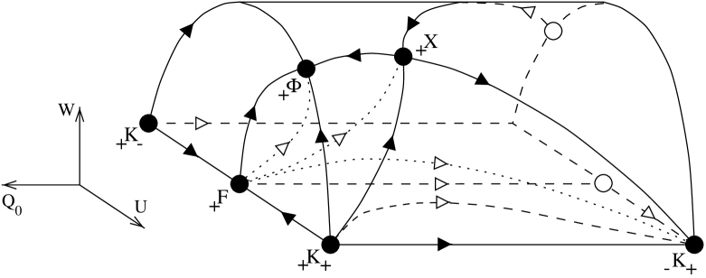
FIG. 1.: The state space for closed FRW models with a scalar field when $\kappa^{2}<2/3$. Dashed curves and white arrows and circles are screened. Dotted orbits are in the interior of the state space.

Table II presents some physical quantities for the various equilibrium points, and Table III lists their eigenvalues. The sources and sinks of the dynamical system when $\gamma>2/3$ are listed in Table IV, and the global behaviour for different values of $\kappa$ can be summarized as follows: The state space when $0<\kappa^{2}<2/3$ is depicted in Fig. 1, where the features in the rear part of the state space have been suppressed. Dashed and full curves represent orbits in the boundary submanifolds, while dotted curves represent orbits in the interior. Both ${}_{+}{\rm K}_{-}$ and ${}_{+}{\rm K}_{+}$ are past attractors, while ${}_{-}{\rm K}_{+}$ and ${}_{+}\Phi$ act as future attractors. There are also orbits from ${}_{+}{\rm K}_{-}$, whose future attractor is ${}_{-}{\rm K}_{-}$ at the rear of the figure. Note that orbits future asymptotic to ${}_{+}\Phi$ correspond to solutions that exhibit power-law inflation ($-1<q_{\rm pf}<0$, see Table II). Observe that the outgoing eigenvector directions from the saddle point ${}_{+}{\rm F}$ span a separatrix surface in the interior of the state space. Similarly, ${}_{+}{\rm X}$ is a saddle for which the ingoing eigenvector directions span another separatrix surface. These separatices confine orbits in the interior state space to specific regions. For example, there is one region where all orbits are past asymptotic to ${}_{+}{\rm K}_{+}$ and future asymptotic to ${}_{-}{\rm K}_{+}$.

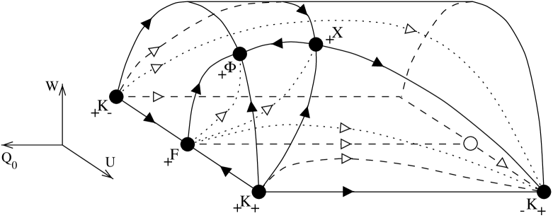
FIG. 2.: The state space for closed FRW models with a scalar field when $2/3<\kappa^{2}<2$. Dashed curves and white arrows and circles are screened. Dotted orbits are in the interior of the state space.

FIG. 3.: Separatrix orbits in the $\Omega_{D}=0$ submanifold of the closed FRW models when $\kappa^{2}$ is near $2/3$. (a) $\kappa^{2}<2/3$; (b) $\kappa^{2}=2/3$; (c) $\kappa^{2}>2/3$.

When $\kappa^{2}>2/3$, the separatrix surface associated with ${}_{+}{\rm X}$ changes structure, see Fig. 2. This is easiest seen by considering the separatrix orbits in the $\Omega_{D}=0$ submanifold, see Fig. 3. When $\kappa^{2}<2/3$, there is one separatrix orbit from ${}_{-}\Phi$ to ${}_{+}{\rm X}$, and one from ${}_{-}{\rm X}$ to ${}_{+}\Phi$. For $\kappa^{2}=2/3$, these two orbits coalesce into a single orbit from ${}_{-}{\rm X}$ to ${}_{+}{\rm X}$. This orbit corresponds to a special “Bouncing Universe” solution, existing only for this particular value of $\kappa$. When $\kappa^{2}>2/3$, the separatrix orbit to ${}_{+}{\rm X}$ starts at ${}_{+}{\rm K}_{-}$, and the orbit from ${}_{-}{\rm X}$ goes to ${}_{-}{\rm K}_{+}$. Thus, there is a bifurcation for $\kappa^{2}=2/3$; however, we note that there is no stability change of equilibrium points involved. A similar behaviour of separatrix surfaces has been found for Bianchi type IX models [13].

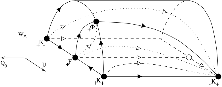
FIG. 4.: The state space for closed FRW models with a scalar field when $2<\kappa^{2}<3\gamma$. Dashed curves and white arrows and circles are screened. Dotted orbits are in the interior of the state space.

When $\kappa$ increases, the equilibrium point ${}_{+}{\rm X}$ approaches ${}_{+}\Phi$. For $\kappa^{2}=2$ these two points coincide, and the state space for $\kappa^{2}>2$ is depicted in Fig. 4. Both ${}_{+}{\rm K}_{-}$ and ${}_{+}{\rm K}_{+}$ still act as past attractors, while ${}_{-}{\rm K}_{+}$ is a future attractor. However, the stability of ${}_{+}\Phi$ has changed; it has become a saddle. There is still a separatrix surface associated with ${}_{+}{\rm F}$. Thus, orbits having ${}_{+}{\rm K}_{+}$ as their past attractor all end at ${}_{-}{\rm K}_{+}$.

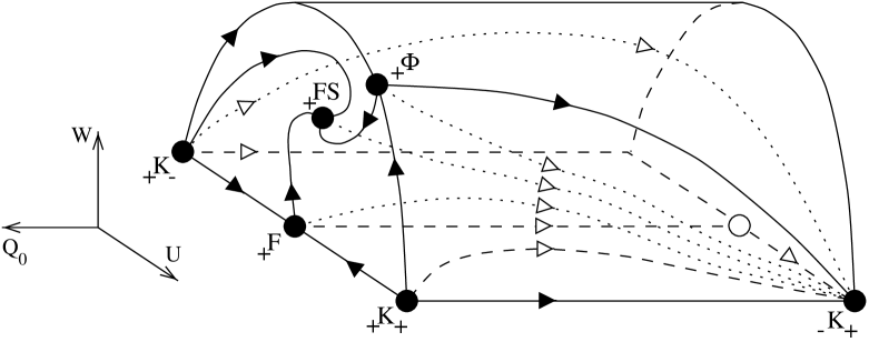
FIG. 5.: The state space for closed FRW models with a scalar field when $3\gamma<\kappa^{2}<6$. Dashed curves and white arrows and circles are screened. Dotted orbits are in the interior of the state space.

For $\kappa^{2}>3\gamma$, the equilibrium point ${}_{+}{\rm FS}$, corresponding to the matter-scaling solution, appears from ${}_{+}\Phi$, see Fig. 5. The point ${}_{+}{\rm FS}$ is a spiral sink with an out-going eigenvector direction entering the interior state space. Note that this equilibrium point thus is stable in the flat ($Q_{0}=1$) submanifold, but unstable to curvature perturbations (i.e., perturbations in the $Q_{0}$ direction). The scalar-field dominated point ${}_{+}\Phi$ still is a saddle, and now there is a separatrix surface spanned by the out-going eigenvector directions there. Thus, there are two separatrix surfaces, both of which are spiraling around the out-going eigenvector direction of ${}_{+}{\rm FS}$.

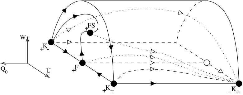
FIG. 6.: The state space for closed FRW models with a scalar field when $\kappa^{2}>6$. Dashed curves and white arrows and circles are screened. Dotted orbits are in the interior of the state space.

When $\kappa$ increases, the ${}_{+}\Phi$ equilibrium point comes closer and closer to ${}_{+}{\rm K}_{+}$, and for $\kappa^{2}=6$ they coincide. The state space when $\kappa^{2}>6$ is given in Fig. 6. There is only one past and one future attractor, namely ${}_{+}{\rm K}_{-}$ and ${}_{-}{\rm K}_{+}$, respectively.

To summarize, when $\kappa^{2}>2$ all solutions start from and recollape to a singularity ($K\rightarrow K$). Thus, in this case solutions can neither expand forever nor inflate. When $\kappa^{2}<2$, there are also ever-expanding (${\rm K}\rightarrow\Phi$) (and ever-collapsing $\Phi\rightarrow{\rm K}$) solutions in addition to the recollapsing solutions. Inflation occurs when $\ddot{S}>0$, i.e., $3\dot{\theta}+\theta^{2}>0$, which leads to the condition

$$-(3\gamma-2)-3(2-\gamma)U^{2}+3\gamma W^{2}>0.$$ (26)

This corresponds to a parabolic region along the ridge of the state spaces, Figs. 1, 2 and 4 – 6. The only equilibrium points within this region are ${}_{\pm}\Phi$ for $\kappa^{2}<2$, corresponding to power-law inflation. Consequently, in the case $\kappa^{2}<2$ there is a subclass of solutions that inflate.

III Kantowski-Sachs models

We now turn our attention to the Kantowski-Sachs (KS) models. The line element can be written

$$ds^{2}=-dt^{2}+D_{1}(t)^{2}dx^{2}+D_{2}(t)^{2}d\Omega^{2},$$ (27)

where

$$D_{1}=\exp\left[\beta^{0}(t)-2\beta^{+}(t)\right],\quad D_{2}=\exp\left[\beta^{0}(t)+\beta^{+}(t)\right].$$ (28)

The kinematic quantities of the fluid congruence are related to the Misner variables ($\beta^{0}$, $\beta^{+}$) by

$$\theta=3\dot{\beta}^{0},\quad\sigma_{+}=3\dot{\beta}^{+},$$ (29)

and the evolution equations for the metric functions $B_{1}\equiv D_{1}^{-1}$ and $B_{2}\equiv D_{2}^{-1}$ become

$$\dot{B}_{1}=-\frac{1}{3}(\theta+\sigma_{+})B_{1},\quad\dot{B}_{2}=-\frac{1}{3}(\theta+\sigma_{+})B_{2}.$$ (30)

The conservation equations give

$$\dot{\mu} = -\gamma\theta\mu,$$ (31)

$$\dot{X} = -\theta X+\frac{\kappa}{\sqrt{2}}V,$$ (32)

and the field equations yield

$$\mu = \frac{1}{3}\left(\theta^{2}-\sigma_{+}^{2}+3B_{2}^{2}-3X^{2}-3V\right),$$ (33)

$$\dot{\theta} = -\frac{1}{3}\left(\theta^{2}+2\sigma_{+}^{2}+6X^{2}-3V+\frac{3}{2}(3\gamma-2)\mu\right),$$ (34)

$$\dot{\sigma}_{+} = \frac{1}{3}\left(\theta^{2}-\sigma_{+}^{2}-3\theta\sigma_{+}-3X^{2}-3V-3\mu\right).$$ (35)

The Friedmann equation, Eq. (33), together with the assumption $\mu\geq 0$ shows that $D=\sqrt{\theta^{2}+3B_{2}^{2}}$ is a dominant quantity. Consequently, compact variables are introduced according to

$$Q_{0}=\frac{\theta}{D},\quad Q_{+}=\frac{\sigma_{+}}{D},\quad U=\frac{\sqrt{3}X}{D},\quad W=\frac{\sqrt{3V}}{D}.$$ (36)

The curvature variable $K=3B_{2}^{2}\,\theta^{-2}=(1-Q_{0}^{2})/Q_{0}^{2}$ shows that the flat solutions correspond to $Q_{0}^{2}=1$. The Friedmann equation becomes

$$\Omega_{D}=\frac{3\mu}{D^{2}}=1-Q_{+}^{2}-U^{2}-W^{2}.$$ (37)

By introducing a new independent variable, $\tau$, where ${}^{\prime}=d/d\tau=\frac{3}{D}\,d/dt$, the evolution equation for $D$,

$$D^{\prime}=-\left[Q_{+}(1-Q_{0}^{2})+3Q_{0}\left(Q_{+}^{2}+U^{2}+\frac{\gamma}{2}\Omega_{D}\right)\right]D,$$ (38)

decouples, and a reduced set of evolution equations is obtained:

$$Q_{0}^{\prime} = (1-Q_{0}^{2})\left[1+Q_{0}Q_{+}-3\left(Q_{+}^{2}+U^{2}+\frac{\gamma}{2}\Omega_{D}\right)\right],$$ (39)

$$Q_{+}^{\prime} = -(1-Q_{0}^{2})(1-Q_{+}^{2})+3Q_{0}Q_{+}\left[-1+\left(Q_{+}^{2}+U^{2}+\frac{\gamma}{2}\Omega_{D}\right)\right],$$ (40)

$$U^{\prime} = U\left\{(1-Q_{0}^{2})Q_{+}+3Q_{0}\left[-1+\left(Q_{+}^{2}+U^{2}+\frac{\gamma}{2}\Omega_{D}\right)\right]\right\}+\sqrt{\frac{3}{2}}\kappa W^{2},$$ (41)

$$W^{\prime} = W\left\{(1-Q_{0}^{2})Q_{+}+3Q_{0}\left(Q_{+}^{2}+U^{2}+\frac{\gamma}{2}\Omega_{D}\right)\right\}-\sqrt{\frac{3}{2}}\kappa UW.$$ (42)

There is also an auxiliary evolution equation:

$$\Omega_{D}^{\prime} = -\Omega_{D}\left\{3\gamma Q_{0}-2\left[Q_{+}(1-Q_{0}^{2})+3Q_{0}\left(Q_{+}^{2}+U^{2}+\frac{\gamma}{2}\Omega_{D}\right)\right]\right\}.$$ (43)

Note that by setting $\kappa=0,U=0$, and identifying $\Lambda=V_{0}$, $\Omega_{\Lambda}=W^{2}$, the evolution equation corresponding to Kantowski-Sachs models with a cosmological constant are obtained [16]. The deceleration parameter is given by

$$q_{\rm pf} = -\frac{1}{Q_{0}^{2}}\left[1-3\left(Q_{+}^{2}+U^{2}+\frac{\gamma}{2}\Omega_{D}\right)\right].$$ (44)

Note that the dynamical system Eqs. (40) is symmetric under the transformation

$$\left(\tau,Q_{0},Q_{+},U,W\right)\rightarrow\left(-\tau,-Q_{0},-Q_{+},-U,W\right).$$ (45)

Thus, it is sufficient to discuss the behaviour in one part of the state space, the dynamics in the other part being obtained by Eq. (45).

The function

$$M = Q_{+}^{-2(3\gamma-2)}(1-Q_{0}^{2})^{-3(2-\gamma)}\Omega_{D}^{4},$$ (46)

$$M^{\prime} = 2Q_{+}^{-1}\left[(3\gamma-2)(1-Q_{0}^{2})+3(2-\gamma)Q_{+}^{2}\right]M$$ (47)

is monotonic in the regions $Q_{+}>0$ and $Q_{+}<0$, since $2/3<\gamma<2$. Noting that

$$\left.Q_{+}^{\prime}\right|_{Q_{+}=0}=-(1-Q_{0}^{2})<0,$$ (48)

we conclude that the submanifold $Q_{+}=0$ is not invariant, but acts as a membrane. Thus, the existence of $M$ rules out any periodic or recurrent orbits in the interior of the state space and again global results are possible. From the expression for the monotonic function $M$ we can immediately see that asymptotically $Q_{+}\rightarrow 0$, $Q_{0}^{2}\rightarrow 1$ or $\Omega_{D}\rightarrow 0$.

A Equilibrium points of the KS dynamical system

The dynamical system, Eqs. (40), has several equilibrium points, which are displayed in Table. V. As before, $\epsilon=\pm 1$ denotes the sign of $Q_{0}$, while $\Omega_{\phi}\equiv U^{2}+W^{2}$. Again, the left subscript gives the sign of $Q_{0}$ and indicates whether the corresponding model is expanding or contracting. The values of $\Omega_{D}$, $\Omega_{\phi}$, and $q_{\rm pf}$ for each of the equilibrium points are given in Table VI while the eigenvalues are displayed in Table VII. Note that all of the equilibrium points correspond to exact self-similar cosmological models [5, 10].

	Interpretation	$Q_{0}$	$Q_{+}$	$U$	$W$	Note
${}_{\pm}{\rm F}$	Flat Friedmann	$\epsilon$	0	0	0
${}_{\pm}{\rm K}$	Kinetic dom.	$\epsilon$	$\pm\sqrt{1-U_{0}^{2}}$	$U_{0}$	0	Ring
${}_{\pm}\Phi$	Scalar-field dom.	$\epsilon$	0	$\frac{\kappa}{\sqrt{6}}\epsilon$	$\frac{1}{\sqrt{6}}\sqrt{6-\kappa^{2}}$	$\kappa^{2}<6$
	(when $\kappa^{2}<2$)
${}_{\pm}\Xi$	Curvature scaling	$2\frac{1+\kappa^{2}}{4+\kappa^{2}}\epsilon$	$-\frac{2-\kappa^{2}}{4+\kappa^{2}}\epsilon$	$\frac{\sqrt{6}\kappa}{4+\kappa^{2}}\epsilon$	$\frac{\sqrt{6}}{4+\kappa^{2}}\sqrt{2+\kappa^{2}}$	$\kappa^{2}<2$
${}_{\pm}{\rm FS}$	Flat matter scaling	$\epsilon$	0	$\sqrt{\frac{3}{2}}\frac{\gamma}{\kappa}\epsilon$	$\sqrt{\frac{3}{2}}\frac{1}{\kappa}\sqrt{\gamma(2-\gamma)}$	$\kappa^{2}>3\gamma$
${}_{\pm}{\rm SSKS}$	Self-similar KS	$\frac{2}{3\gamma-4}\epsilon$	$\frac{3\gamma-2}{3\gamma-4}\epsilon$	0	0	$\gamma<2/3$

TABLE V.: Equilibrium points of the KS models.

As for the closed FRW models, ${}_{\pm}{\rm F}$ denotes the flat Friedmann solution. Note that the closed FRW solution without a scalar field does not appear as a submanifold of the Kantowski-Sachs models without a scalar field. Consequently, there is no orbit connecting ${}_{+}{\rm F}$ with ${}_{-}{\rm F}$.

There are two sets ${}_{\pm}{\rm K}$ of vacuum ($\Omega_{D}=0$) equilibrium points, parameterized by the constant $U_{0}$, corresponding to kinetic dominated solutions. These sets are analogues of the “Kasner rings” that are present for various Bianchi models.

The flat scalar-field dominated points ${}_{\pm}\Phi$, already encountered for the closed FRW models, appear in the Kantowski-Sachs case as well. As for the closed FRW models, they are physical when $\kappa^{2}<6$ and inflationary when $\kappa^{2}<2$.

There are also equilibrium points ${}_{\pm}\Xi$, corresponding to curvature scaling solutions (i.e. they have $\Omega_{D}=0$, $Q_{0}^{2}<1$) which are physical when $\kappa^{2}<2$. They are also inflationary, but in other respects they resemble the points ${}_{\pm}{\rm X}$ of the closed FRW models.

As for the closed FRW models, the equilibrium points ${}_{\pm}{\rm FS}$, corresponding to the flat matter-scaling solution, enter the physical part of the state space when $\kappa^{2}>3\gamma$.

Finally, there are also equilibrium points corresponding to the self-similar Kantowski-Sachs solution. This solution is only physical when $\gamma<2/3$, and so we will not consider them further.

	$\Omega_{D}$	$\Omega_{\phi}$	$q_{\rm pf}$
${}_{\pm}{\rm F}$	1	0	$\frac{1}{2}(3\gamma-2)$
${}_{\pm}{\rm K}$	0	$U_{0}^{2}$	2
${}_{\pm}\Phi$	0	1	$\frac{1}{2}(\kappa^{2}-2)$
${}_{\pm}\Xi$	0	$12\frac{1+\kappa^{2}}{(4+\kappa^{2})^{2}}$	$\frac{1}{2}\frac{\kappa^{2}-2}{1+\kappa^{2}}$
${}_{\pm}{\rm FS}$	$\frac{\kappa^{2}-3\gamma}{\kappa^{2}}$	$\frac{3\gamma}{\kappa^{2}}$	$\frac{1}{2}(3\gamma-2)$
${}_{\pm}{\rm SSKS}$	$-12\frac{\gamma-1}{(3\gamma-4)^{2}}$	0	$\frac{1}{2}(3\gamma-2)$

TABLE VI.: The physical quantities $\Omega_{D}$, $\Omega_{\phi}$, and $q_{\rm pf}$ for the different equilibrium points of the KS models.

	Eigenvalues
${}_{\pm}{\rm F}$	$(3\gamma-2)\epsilon$	$-\frac{3}{2}(2-\gamma)\epsilon$	$-\frac{3}{2}(2-\gamma)\epsilon$	$\frac{3\gamma}{2}\epsilon$
${}_{\pm}{\rm K}$	$4\epsilon-2Q_{+}$	$3(2-\gamma)\epsilon$	0	$3\epsilon-\sqrt{\frac{3}{2}}\kappa U_{0}$
${}_{\pm}\Phi$	$-\frac{1}{2}(6-\kappa^{2})\epsilon$	$-\frac{1}{2}(6-\kappa^{2})\epsilon$	$-(2-\kappa^{2})\epsilon$	$-(3\gamma-\kappa^{2})\epsilon$
${}_{\pm}\Xi$	$-3\frac{2+\kappa^{2}}{4+\kappa^{2}}\epsilon$	$-6\frac{\gamma+(\gamma-1)\kappa^{2}}{4+\kappa^{2}}\epsilon$	$-\frac{3}{2}\frac{2+\kappa^{2}\pm\sqrt{(2+\kappa^{2})(18-7\kappa^{2})}}{4+\kappa^{2}}\epsilon$
${}_{\pm}{\rm FS}$	$-\frac{3}{2}(2-\gamma)\epsilon$	$(3\gamma-2)\epsilon$	$-\frac{3}{4\kappa}\left[(2-\gamma)\kappa\pm\sqrt{(2-\gamma)(24\gamma^{2}-(9\gamma-2)\kappa^{2})}\right]\epsilon$
${}_{\pm}{\rm SSKS}$	$-3\frac{2-\gamma}{3\gamma-4}\epsilon$	$\frac{3\gamma}{3\gamma-4}\epsilon$	$-\frac{3}{2}\frac{2-\gamma\pm\sqrt{(2-\gamma)(24\gamma^{2}-41\gamma+18)}}{3\gamma-4}\epsilon$

TABLE VII.: Eigenvalues for the different equilibrium points of the KS models.

Past attractors
Expanding from a singularity ($Q_{0}>0$)	${}_{+}{\rm K}$	$\kappa U_{0}<\sqrt{6}$
Contracting from a dispersed state ($Q_{0}<0$)	${}_{-}\Phi$	$\kappa^{2}<2$
Future attractors
Contracting to a singularity ($Q_{0}<0$)	${}_{-}{\rm K}$	$\kappa U_{0}<\sqrt{6}$
Expanding to a dispersed state ($Q_{0}>0$)	${}_{+}\Phi$	$\kappa^{2}<2$

TABLE VIII.: Summary of sources and sinks for the KS models.

The eigenvalues for each of the equilibrium points are given in Table VII. The sources and sinks of the dynamical system when $\gamma>2/3$ are listed in Table VIII (all of the other equilibrium points are saddles). Thus, there is always two segments of the equilibrium set ${}_{+}{\rm K}$ that act as sources for orbits. Similarly there are two segments on ${}_{-}{\rm K}$ that are sinks. When $\kappa^{2}>2$, these are the only attractors, and all solutions start from and recollape to a singularity ($K\rightarrow K$).

When $\kappa^{2}<2$, which then implies that $\kappa^{2}<3\gamma$ for $\gamma>2/3$, the equilibrium points ${}_{\pm}\Phi$ are attractors. Thus, for $\kappa^{2}<2$, there are also ever-expanding (${}_{+}{\rm K}\rightarrow{{}_{+}\Phi}$) and ever-collapsing (${}_{-}\Phi\rightarrow{{}_{-}{\rm K}}$) solutions.

From the expression for the monotonic function $M$ we deduce that all orbits asymptotically have $Q_{+}\rightarrow 0$, $Q_{0}^{2}\rightarrow 1$ or $\Omega_{D}\rightarrow 0$. Indeed, the existence of the monotonic function ensures that there are no periodic orbits and that generically orbits asymptote towards the local attractors (sinks and sources). Therefore, we can determine the global dynamics of the models.

To summarize, when $\kappa^{2}>2$ all solutions start from and recollape to a singularity ($K\rightarrow K$). Thus, in this case solutions can neither isotropize nor inflate. When $\kappa^{2}<2$, there are also ever-expanding (${\rm K}\rightarrow\Phi$) (and ever-collapsing $\Phi\rightarrow{\rm K}$) solutions in addition to the recollapsing solutions. Again, the $\Phi$ points correspond to power-law inflation when $\kappa^{2}<2$. Consequently, in this case there is a subclass of solutions that isotropize and inflate.

The global asymptotic dynamics is similar to that in the case of positive-curvature FRW models. However, due to the presence of shear, the intermediate or transient dynamics can be quite different. In the Kantowski-Sachs case the state space is four-dimensional and so we cannot display the phase portraits graphically (as in the FRW case). However, as an illustration we shall present the phase portraits in the three-dimensional fluid vacuum and the massless scalar field invariant sets in order to compare intermediate behaviours.

B Fluid vacuum

The fluid vacuum ($\Omega_{D}=0$) is an invariant submanifold, as seen from Eq. (43). Using the Friedmann equation to eliminate $W$, we obtain a three-dimensional dynamical system in $(Q_{0},Q_{+},U)$:

$$Q_{0}^{\prime} = (1-Q_{0}^{2})\left[1+Q_{0}Q_{+}-3(Q_{+}^{2}+U^{2})\right],$$ (49)

$$Q_{+}^{\prime} = -(1-Q_{0}^{2})(1-Q_{+}^{2})-3Q_{0}Q_{+}(1-Q_{+}^{2}-U^{2}),$$ (50)

$$U^{\prime} = (1-Q_{0}^{2})Q_{+}U+\left(\sqrt{\frac{3}{2}}\kappa-3Q_{0}U\right)(1-Q_{+}^{2}-U^{2}).$$ (51)

From table VI, it is immediately seen that the equilibrium points that are contained in this submanifold are ${}_{\pm}{\rm K}$, ${}_{\pm}\Phi$, and ${}_{\pm}\Xi$. The state space is depicted in Figs. 7, 8 and 9. Note that $Z=0$, where $Z$ is defined by

$$Z=Q_{+}-\frac{1}{2}Q_{0}+\frac{\sqrt{6}}{2\kappa}U,$$ (52)

is an invariant submanifold, and that both ${}_{\pm}\Phi$ and ${}_{\pm}\Xi$ are contained in this submanifold.

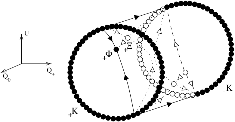
FIG. 7.: The state space for Kantowski-Sachs models with no fluid ($\Omega_{D}=0$), with $\kappa^{2}<2$. Dashed curves and white arrows and circles are screened. Dotted orbits lie in the $Z=0$ invariant submanifold.

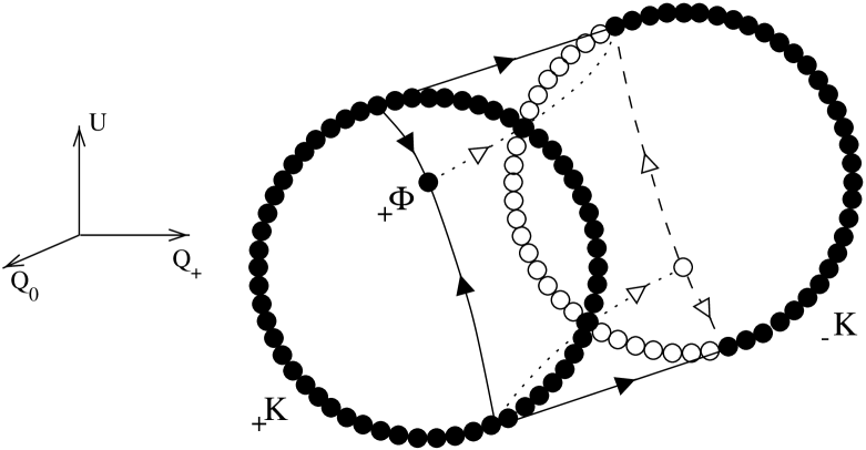
FIG. 8.: The state space for Kantowski-Sachs models with no fluid ($\Omega_{D}=0$), with $2<\kappa^{2}<6$. Dashed curves and white arrows and circles are screened. Dotted orbits lie in the $Z=0$ invariant submanifold.

FIG. 9.: The state space for Kantowski-Sachs models with no fluid ($\Omega_{D}=0$), with $\kappa^{2}>6$. Dashed curves and white arrows and circles are screened.

C Massless case

The massless case corresponds to the invariant submanifold $W=0$, which leads to a three-dimensional system in ($Q_{0},Q_{+},U$):

$$Q_{0}^{\prime} = -(1-Q_{0}^{2})\left[\frac{3\gamma-2}{2}-Q_{0}Q_{+}+\frac{3}{2}(2-\gamma)(Q_{+}^{2}+U^{2})\right],$$ (53)

$$Q_{+}^{\prime} = -(1-Q_{0}^{2})(1-Q_{+}^{2})-\frac{3}{2}(2-\gamma)Q_{0}Q_{+}\Omega_{D},$$ (54)

$$U^{\prime} = U\left[(1-Q_{0}^{2})Q_{+}-\frac{3}{2}(2-\gamma)Q_{0}\Omega_{D}\right].$$ (55)

From table V, it is immediately seen that the equilibrium points that are contained in this submanifold are ${}_{\pm}{\rm K}$ and ${}_{\pm}{\rm F}$. The state space is depicted in Fig. 10.

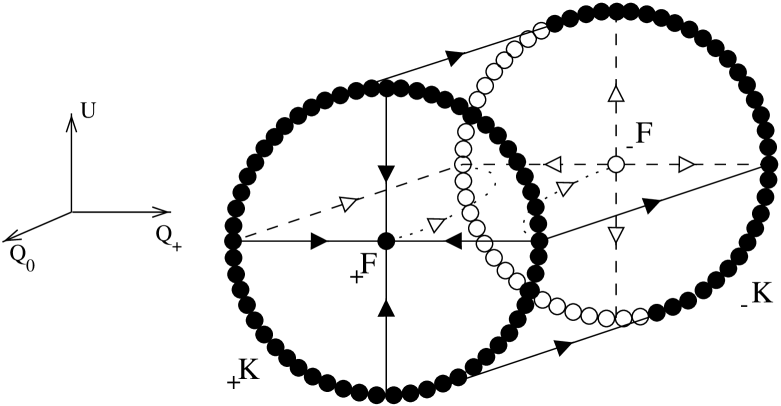
FIG. 10.: The state space for Kantowski-Sachs models with fluid and massless scalar field, $W=0$. Dashed curves and white arrows and circles are screened. The horizontal plane is the $U=0$ invariant submanifold (compare with [21]).

IV Discussion

We have studied closed cosmological models with a perfect fluid satisfying a linear equation of state with $2/3<\gamma<2$ and a scalar field with an exponential potential. We have utilized a new set of normalised variables which lead to the compactification of state space, enabling us to apply the theory of dynamical systems to determine the qualitative properties of the models. In all cases we have been able to find monotonic functions which, together with a local analysis of the equilibrium points, enable us to determine the global properties of the models.

We first studied the closed FRW cosmological models. We found that when $\kappa^{2}>2$, all solutions start from and recollape to a singularity ($K\rightarrow K$). In this case solutions generically do not inflate. When $\kappa^{2}<2$, solutions can either recollapse ($K\rightarrow K$) or expand forever (${\rm K}\rightarrow\Phi$) towards power-law inflation solutions (or collapse forever $\Phi\rightarrow{\rm K}$); consequently, in this case there is a subclass of solutions that inflate. A number of phase portraits were displayed.

These results generalise previous qualitative work on positive-curvature FRW models with a scalar field (only) [9] and with a scalar field plus a barotropic perfect fluid [8] in which compactified variables were not utilized, and rigorous analyses of perfect fluid (only) models using compactified variables [10, 11], and completes and generalises more recent work using different compactified variables [17]. We also note that positive-curvature FRW models with a perfect fluid and a positive cosmological constant have been investigated recently using qualitative methods and utilizing compactified variables [16].

In the case of the Kantowski-Sachs models we again found that when $\kappa^{2}>2$ all solutions start from and recollape to a singularity ($K\rightarrow K$) and can consequently neither isotropize nor inflate. When $\kappa^{2}<2$, there are also ever-expanding (${\rm K}\rightarrow\Phi$) (and ever-collapsing $\Phi\rightarrow{\rm K}$) solutions in addition to the recollapsing solutions, where again the $\Phi$ points correspond to the flat FRW power-law inflationary solution. Consequently, in this case there is a subclass of solutions that isotropize and inflate.

The investigation of Kantowski-Sachs models complements the study of Bianchi models [5] and completes the analysis of spatially homogeneous models. Collins [22] studied perfect fluid Kantowski-Sachs models qualitatively using expansion-normalised variables (for which the state space was non-compact) and showed that all models start at a Big Bang and recollapse to a final “Big Crunch” singularity. This work was generalised recently by Goliath and Ellis [16] in which Kantowski-Sachs models with a perfect fluid and a cosmological constant were investigated using qualitative methods and utilizing the compactified variables of Uggla and Zur-Muhlen [13]; particular attention was focussed upon whether the models isotropize, thereby explaining the presently observed near-isotropy of the universe. More importantly, Kantowski-Sachs models with a scalar field and an exponential potential, but without barotropic matter, have been studied qualitatively [12], although compactified variables were not utilized.

To conclude an analysis of positive-curvature spatially homogeneous cosmological models with a perfect fluid and a scalar field with an exponential potential, Bianchi type IX models would need to be studied. However, such a study is beyond the scope of the current paper. For example, Bianchi type IX models are known to have very complicated dynamics, exhibiting the characteristics of chaos [10, 15]. However, partial results are known. Bianchi type IX models with a scalar field (only) have been studied qualitatively, with an emphasis on whether these models can isotropize [14]. Scalar-field models with matter have also been studied [3]. For example, it has been shown that the power-law inflationary solution is an attractor for all initially expanding Bianchi type IX models except for a subclass of the models which recollapse [3, 4]. However, compact variables have not been utilized and the analyses were not rigorous.

A more rigorous treatment of the class of Bianchi type IX models with a non-tilted perfect fluid (only) using compactified variables has been possible [10]. Although an appropriately defined normalised Hubble variable is found to be monotonic, enabling some results to be obtained, several problems remain open. More rigorous global results are possible. For example, Bianchi type IX models with matter have been shown to obey the “closed universe recollapse” conjecture [23], whereby initially expanding models enter a contracting phase and recollapse to a future “Big Crunch”. In addition, Ringström has proven that a curvature invariant is unbounded in the incomplete directions of inextendible null geodesics for generic vacuum Bianchi models [24], and rigorously shown that the Mixmaster attractor is the past attractor of Bianchi type IX models with an orthogonal perfect fluid [25]. A complete qualitative analysis of the special class of locally rotationally symmetric Bianchi type IX perfect fluid models, which do not exhibit oscillatory or chaotic behaviour near to the initial or final singularities, has been given in [13], based upon an appropriately defined set of bounded variables.

The Kantowski-Sachs models exhibit similar global properties to the positive-curvature FRW models; in particular, for $\kappa^{2}>2$ all initially expanding models reach a maximum expansion and thereafter recollapse, whereas for $\kappa^{2}<2$ models generically recollapse or expand forever towards a flat isotropic power-law inflationary solution. The Bianchi type IX models share these qualitative properties. However, the intermediate behaviour of the Kantowski-Sachs models can be quite different to that of the FRW models. In order to illustrate the possible intermediate dynamics of the Kantowski-Sachs models, we studied the special cases of no barotropic fluid, and a massless scalar field in Secs. III B and III C, respectively (see Figs. 7 – 10).

Finally, we remark that the dynamics of the Kantowski-Sachs models obtained here will be crucial for understanding the global dynamics of general self-similar spherically symmetric models [20].

V Acknowledgements

We would like to thank Peter Turner for his help with the analysis of the positive-curvature FRW models [17]. AC would like to acknowledge financial support from NSERC of Canada. MG would like to thank the Department of Mathematics and Statistics at Dalhousie University for hospitality while this work was carried out.

REFERENCES

- [1] M. B. Green, J. H. Schwarz, and E. Witten, Superstring Theory (Cambridge University Press, Cambridge, 1987).
- [2] N. Kaloper, R. Madden, and K. A. Olive, Nucl. Phys. B452, 677 (1995).
- [3] Y. Kitada and K. Maeda, Phys. Rev. D 45, 1416 (1992); Y. Kitada and K. Maeda, Class. Quantum Grav. 10, 703 (1993).
- [4] A. A. Coley, J. Ibáñez, and R. J. van den Hoogen, J. Math. Phys 38, 5256 (1997).
- [5] A. P. Billyard, A. A. Coley, R. J. van den Hoogen, J. Ibáñez, and I. Olasagasti, Class. Quantum Grav. 16, 4035 (1999).
- [6] E. J. Copeland, A. R. Liddle, and D. Wands, Phys. Rev. D 57, 4686 (1998).
- [7] A. P. Billyard, A. A. Coley, and R. J. van den Hoogen, Phys. Rev. D 58, 123501 (1998).
- [8] R. J. van den Hoogen, A. A. Coley, and D. Wands, Class. Quantum Grav. 16, 1843 (1999).
- [9] J. J. Halliwell, Phys. Letts. B 185, 341 (1987).
- [10] J. Wainwright and G. F. R. Ellis, Dynamical Systems in Cosmology (Cambridge University Press, Cambridge, 1997).
- [11] J. Wainwright, in G. S. Hall and J. R. Pulham (eds.) Proceedings of the forty sixth Scottish universities summer school in physics, Aberdeen (Institute of physics publishing, London, 1996).
- [12] A. B. Burd and J. D. Barrow, Nucl. Phys. B308, 929 (1988).
- [13] C. Uggla and H. von zur Mühlen, Class. Quantum Grav. 7, 1365 (1990).
- [14] R. J. van den Hoogen and I. Olasagasti, Phys. Rev. D 59, 107302 (1999).
- [15] D. Hobill, A. Burd, and A. Coley (Eds.), Deterministic chaos in general relativity, NATO ASI series B, vol. 332 (Plenum Press, New York, 1994).
- [16] M. Goliath and G. F. R. Ellis, Phys. Rev. D 60, 023502 (1999).
- [17] P. Turner, Honours Thesis Project (Dalhousie University 1999).
- [18] O. I. Bogoyavlensky, Methods in the qualitative theory of dynamical systems in astrophysics and gas dynamics, (Springer, Berlin 1985).
- [19] B. J. Carr, A. A. Coley, M. Goliath, U. S. Nilsson, and C. Uggla, preprint gr-qc/9902070 (1999).
- [20] A. A. Coley and M. Goliath, preprint gr-qc/0003080, to appear in Class. Quantum Grav. (2000).
- [21] M. Goliath, U. S. Nilsson, and C. Uggla, Class. Quantum Grav. 15, 167 (1998).
- [22] C. B. Collins, J. Math. Phys. 18, 2116 (1977).
- [23] X. F. Lin and R. M. Wald, Phys. Rev. D 40, 3280 (1989); ibid. 41, 2444 (1989).
- [24] H. Ringström, Class. Quantum Grav. 17, 713 (2000).
- [25] H. Ringström, in preparation.