The Innermost Stable Circular Orbit of Binary Black Holes

Abstract

We introduce a new method to construct solutions to the constraint equations of general relativity describing binary black holes in quasicircular orbit. Black hole pairs with arbitrary momenta can be constructed with a simple method recently suggested by Brandt and Brügmann, and quasicircular orbits can then be found by locating a minimum in the binding energy along sequences of constant horizon area. This approach produces binary black holes in a ”three-sheeted” manifold structure, as opposed to the ”two-sheeted” structure in the conformal-imaging approach adopted earlier by Cook. We focus on locating the innermost stable circular orbit and compare with earlier calculations. Our results confirm those of Cook and imply that the underlying manifold structure has a very small effect on the location of the innermost stable circular orbit.

]

I INTRODUCTION

Binary black holes are among the most promising sources of gravitational radiation for the new generation of gravitational wave detectors such as the Laser Interferometric Gravitational Wave Observatory (LIGO), VIRGO, GEO and TAMA. This has motivated an intense theoretical effort to predict the gravitational waveform emitted during the inspiral and coalescence of two black holes [1].

Because of the circularizing effects of gravitational radiation damping, we expect the orbits of close binary systems to have small eccentricities. The inspiral of a binary black hole system then proceeds adiabatically along a sequence of quasicircular orbits up to the innermost stable circular orbit (hereafter ISCO), where the evolution is expected to change into a rapid plunge and coalescence[2]. The ISCO therefore leaves a characteristic signature in the gravitational wave signal, and knowledge of its location and frequency is thus very important for the prospect of future observations.

While various approximations may be adequate to model the adiabatic inspiral up to the ISCO, it is generally expected that only numerical simulations in full general relativity can accurately model the dynamical plunge and merger and predict the gravitational signal from that phase. It is therefore desirable to construct initial data for numerical evolution calculations describing binary black hole pairs at the ISCO, which adds another motivation for determining the location of the ISCO.

Various approaches have been adopted to locate the ISCO in compact binaries, including first order post-Newtonian approximations [5], variational principles [6], second order post-Newtonian methods combined with a “hybrid” approach [7], a Padé approximation [8] and an effective-one-body approach [9, 3], and numerical solutions to the constraint equations of general relativity [10, 11]. Unfortunately, however, the results differ significantly and yet have to show any sign of convergence (see Table II below). It would clearly be desirable to understand the origin of these differences. In this paper, we revisit binary black hole solutions to the constraint equations, and evaluate how some of the choices which have to be made in this approach affect the location of the ISCO.

Before the constraint equations of general relativity can be solved, a background geometry and topology have to be chosen. In the conformal-imaging approach adopted by Cook [10], a conformally flat (spatial) background metric is chosen together with a two-sheeted manifold structure (see Sec. II A). It has been suggested that these choices may affect the location of the ISCO, and may explain the difference between these and the more recent post-Newtonian results.

In this paper, we combine the methods of Cook [10] and Brandt and Brügmann [12] to introduce a new approach to constructing binary black holes in quasicircular orbit. We follow Cook [10] and choose a conformally flat background metric, but do not assume an inversion-symmetry as is done in the conformal-imaging approach. This considerably simplifies the solution of the momentum constraint (see Sec. II B), and produces binary black holes in a three-sheeted manifold structure as opposed to the two-sheeted structure in the conformal-imaging approach. Moreover, adopting the “puncture” approach of Brandt and Brügmann [12], the Hamiltonian constraint can be solved very easily numerically on R³ without having to impose boundary conditions on interior boundaries (see Sec. II C). We locate the ISCO, and find that its physical parameters agree very well with those found with the conformal-imaging approach of Cook [10]. We therefore conclude that the choice of the underlying manifold structure has a very small effect on the location of the ISCO. Our new approach, which is significantly simpler than the conformal-imaging approach, may also provide a framework in which the conformal-flatness assumption may be relaxed, and its effect on the ISCO be evaluated.

The paper is organized as follows. In Sec. II, we introduce the basic equations and explain how binary black holes in quasicircular orbit can be constructed. We discuss our numerical implementation in Sec. III. In Sec. IV we present our results and compare with those from other approaches. We briefly summarize in Sec. V.

II SETUP OF THE PROBLEM

A The Initial Value Problem

A framework for constructing initial data describing binary black holes has been provided by Arnowitt, Deser and Misner’s $3+1$ decomposition of Einstein’s equations [13] and York’s conformal decomposition [14, 15].

The $3+1$ decomposition splits Einstein’s equations into evolution and constraint equations for the metric $\gamma_{ij}$ of a spatial hypersurface $\Sigma$, and the extrinsic curvature $K_{ij}$, which describes the embedding of the hypersurface $\Sigma$ in the full spacetime. The physical metric $\gamma_{ij}$ can now be decomposed into a conformal factor $\psi$ and a conformal background metric $\hat{\gamma}_{ij}$,

$$\gamma_{ij}=\psi^{4}\hat{\gamma}_{ij}.$$ (1)

It is also convenient to decompose the extrinsic curvature $K_{ij}$ into its trace $K$ and a trace-free conformal background extrinsic curvature $\hat{A}_{ij}$ according to

$$K_{ij}=\psi^{-2}\hat{A}_{ij}+\frac{1}{3}\gamma_{ij}K.$$ (2)

The Hamiltonian constraint then reduces to an equation for the conformal factor $\psi$,

$$8\hat{\nabla}^{2}\psi-\psi\hat{R}-\frac{2}{3}\psi^{5}K^{2}+\psi^{-7}\hat{A}_{ij}\hat{A}^{ij}=0,$$ (3)

and the momentum constraint can be written

$$\hat{D}_{j}\hat{A}^{ij}-\frac{2}{3}\psi^{6}\hat{\gamma}^{ij}\hat{D}_{j}K=0.$$ (4)

Here $\hat{D}_{i}$ is the covariant derivative compatible with the conformal background metric, $\hat{\nabla}^{2}$ the Laplacian, and $\hat{R}$ is the Ricci scalar.

Binary black hole initial data cannot be constructed uniquely, because the constraint equations of general relativity determine neither the background geometry nor the topology of the spacetime, both of which have to be chosen before the constraint equations can be solved. Loosely speaking, these ambiguities correspond to different amounts of gravitational radiation in the initial data sets. In this paper, we will follow Cook et.al. [10, 16, 17] and choose a flat background geometry, but we will choose a three-sheeted topology as opposed to the two-sheeted topology of Cook.

Choosing the background geometry amounts to choosing the conformal background metric $\hat{\gamma}_{ij}$. Following Cook et.al. [10, 16, 17], we choose the conformal background geometry to be flat so that $\hat{\gamma}_{ij}=f_{ij}$, where $f_{ij}$ is the flat metric in a so far arbitrary coordinate system. The covariant derivative $\hat{D}_{i}$ then becomes the flat-space covariant derivative, and the Ricci scalar $\hat{R}$ vanishes. We will later specialize to cartesian coordinates, $\hat{\gamma}_{ij}=\delta_{ij}$, for which $\hat{D}_{i}$ reduces to a partial derivative. We also take the hypersurface $\Sigma$ to be maximally embedded in the spacetime so that $K=0$. With these choices, the constraint equations simplify to

$$\hat{\nabla}^{2}\psi=-\frac{1}{8}\psi^{-7}\hat{A}_{ij}\hat{A}^{ij}$$ (5)

and

$$\hat{D}_{j}\hat{A}^{ij}=0.$$ (6)

Note that maximal slicing $K=0$ automatically decouples the momentum constraint from the Hamiltonian constraint.

Choosing the topology of the spacetime is less straight-forward (compare the discussion in [16]). Since we are interested in isolated black-holes systems, it is natural to assume the hypersurface $\Sigma$ to be asymptotically flat. Constructing black hole data in vacuum, however, necessarily involves non-trivial topologies. This can be illustrated by a $t=const$ slice of the Schwarzschild geometry in isotropic coordinates, where every point inside the black hole’s throat can be mapped into a point outside the throat and vice versa. Moreover, such a mapping can be accomplished with an isometry, which maps the metric into itself, implying that the physical fields at a point inside the throat are identical to those at a point outside the throat. In particular, the geometry near the center is identical to the geometry near infinity. We can therefore think of this solution as describing two identical, asymptotically flat “universes” or “sheets”, which are connected by a throat or Einstein-Rosen bridge [18].

There is no unique generalization of this topology to the case of multiple black holes [19]. For two black holes, the two throats could either connect to the same asymptotically flat sheet, or else to two separate asymptotically flat sheets. The former approach results in a two-sheeted topology, the latter in a three-sheeted topology.

Cook et.al. [10, 16, 17] implemented a “conformal-imaging” formalism, which adopts a two-sheeted topology together with the additional demand that the two sheets are related by an isometry so that their physical fields are identical (cf. [20, 21]). It has been argued that this choice is the “most faithful generalization of the Schwarzschild geometry to the case of multiple holes” [16]. Moreover, the isometry conditions on the throats can be used as boundary conditions in numerical implementations, so that singularities inside the throats can be eliminated from the numerical grid. The computational disadvantage of this method is that boundary conditions have to be imposed on fairly complicated surfaces. In finite difference algorithms, this can be accomplished either with bispherical or Čadež coordinates [22], designed such that a constant coordinate surface coincides with the throat, or else with fairly complicated algorithms in cartesian coordinates. Both approaches, together with a spectral method, have been compared in [17].

In this paper, we choose instead a three-sheeted topology and do not assume an inversion-symmetry across the throats, which simplifies the problem in two respects. The analytical solution to the momentum constraint becomes very simple, since we no longer need to construct inversion-symmetric solutions (see Sec. II B). Moreover, the singularities inside the black holes can be removed analytically using a “puncture” method recently suggested by Brandt and Brügmann [12] (see Sec. II C). The problem can then be solved quite easily on R³ in cartesian coordinates, without having to impose interior boundary conditions. The only added complication is that one now has to locate apparent horizons in the numerically constructed hypersurface.

B Solving the Momentum Constraint for Binary Black Holes

For maximally sliced hypersurfaces, the momentum constraint decouples from the conformal factor, and analytical solutions to (6) can be given. Moreover, for conformally and asymptotically flat data, the total (physical) linear momentum [23]

$$P^{i}=\frac{1}{8\pi}\oint_{\infty}\hat{A}^{ij}d^{2}S_{j}$$ (7)

and the total (physical) angular momentum

$$J_{i}=\frac{\epsilon_{ijk}}{8\pi}\oint_{\infty}x^{j}\hat{A}^{kl}d^{2}S_{l}$$ (8)

can be determined from $\hat{A}^{ij}$ without having to solve the Hamiltonian constraint (5) (see [24]).

Analytical solutions to the momentum constraint (6) describing single boosted or spinning black holes have been given by Bowen and York [24, 25, 26]. A solution $\hat{A}^{ij}$, describing a single black hole at the coordinate location ${\bf C}$ with linear momentum ${\bf P}$ is given by

$$\hat{A}^{ij}_{\bf CP}=\frac{3}{2r^{2}_{\bf C}}\left(P^{i}n^{j}_{\bf C}+P^{j}n^{i}_{\bf C}+(f^{ij}+n^{i}_{\bf C}n^{j}_{\bf C})P_{k}n^{k}_{\bf C}\right).$$ (9)

Here $r_{\bf C}=\|x^{i}-C^{i}\|$ is the coordinate distance to the center of the black hole and $n^{i}_{\bf C}=(x^{i}-C^{i})/r$ is the normal vector pointing away from that center. Additional terms have to be added in the conformal-imagine approach for an isometry condition to hold across the throat. Note that we have only included linear momentum terms in this expression, and that we are therefore restricting our analysis to non-spinning black holes.

Since the momentum constraint (6) is linear, we can construct binary black hole solutions by superposition of single solutions

$$\hat{A}^{ij}=\hat{A}^{ij}_{{\bf C}_{1}{\bf P}_{1}}+\hat{A}^{ij}_{{\bf C}_{2}{\bf P}_{2}}.$$ (10)

From (7) and (8) we find the that total momentum of this solution is ${\bf P}={\bf P}_{1}+{\bf P}_{2}$, and the angular momentum about the origin of the coordinate system

$${\bf J}={\bf C}_{1}{\bf\times P}_{1}+{\bf C}_{2}{\bf\times P}_{2}.$$ (11)

Note that constructing inversion-symmetric solutions for multiple black holes in the conformal-imaging approach is fairly complicated. There, the components of the extrinsic curvature are expressed in terms of an infinite series of recursively defined quantities (see [21] and Appendix A of [10]). Relaxing the inversion symmetry, so that the extrinsic curvature can be written as a simple superposition of two solutions (9), therefore greatly simplifies the problem.

C Solving the Hamiltonian Constraint for Binary Black Holes

Solutions to the Hamiltonian constraint (5) can be constructed by generalizing the Schwarzschild solution in isotropic coordinates for a static (i.e. $\hat{A}_{ij}=0$) and spherically symmetric black hole at coordinate location ${\bf C}$,

$$\psi=1+\frac{{\cal M}}{2r_{\bf C}}$$ (12)

(note that asymptotic flatness demands $\psi\rightarrow 1$ as $r\rightarrow\infty$). Solutions describing multiple static black holes can be constructed by adding contributions ${\cal M}/(2r_{\bf C})$ for each black hole. To establish an inversion-symmetry, additional terms would again have to be added [20].

In the “puncture” method suggested by Brandt and Brügmann [12], a general nonstatic solution to the Hamiltonian constraint is written as a sum of the static, analytic contribution plus a term correcting for finite $\hat{A}_{ij}$. Adopting their notation, we write

$$\psi=u+\frac{1}{\alpha},$$ (13)

where $\alpha$ is defined by

$$\frac{1}{\alpha}=\frac{{\cal M}_{1}}{2r_{{\bf C}_{1}}}+\frac{{\cal M}_{2}}{2r_{{\bf C}_{2}}}.$$ (14)

The Hamiltonian constraint then becomes an equation for the correction term $u$

$$\hat{\nabla}^{2}u=-\beta\,(1+\alpha u)^{-7},$$ (15)

where we have abbreviated

$$\beta=\frac{1}{8}\,\alpha^{7}\,K_{ij}K^{ij}.$$ (16)

For asymptotic flatness, we impose a Robin boundary condition $\partial(r\,(u-1))/\partial r=0$ at large distances from the black holes. The existence and uniqueness of solutions $u$ on R³ has been established in [12]. The beauty of this approach is that the poles at the center of the black holes have been absorbed into the analytical terms. The corrections $u$ are regular everywhere and can be solved for very easily on a simple computational domain, without having to impose boundary conditions on the throats.

Once the conformal factor $\psi$ has been determined, the ADM mass of the solution can be found from

$$E = -\frac{1}{2\pi}\oint_{\infty}\hat{\nabla}^{i}\psi\,d^{2}S_{i}$$ (17)

$$= -\frac{1}{2\pi}\oint_{\infty}\hat{\nabla}^{i}\left(\frac{1}{\alpha}\right)d^{2}S_{i}-\frac{1}{2\pi}\int\hat{\nabla}^{2}u\,dV$$ (18)

$$= {\cal M}_{1}+{\cal M}_{2}+\frac{1}{2\pi}\int\beta\,(1+\alpha u)^{-7}dV.$$ (19)

Note that the integral extends over all space.

D Constructing Equal-mass Binary Black Holes in Quasicircular Orbit

We now specialize to equal mass black holes with ${\cal M}\equiv{\cal M}_{1}={\cal M}_{2}$. In the center-of-mass frame of the binary system, we have

$${\bf P}\equiv{\bf P}_{1}=-{\bf P}_{2}.$$ (20)

Binaries in quasicircular orbit should furthermore satisfy ${\bf P\cdot C}=0$, where we have defined

$${\bf C}\equiv{\bf C}_{1}-{\bf C}_{2}.$$ (21)

Without loss of generality, we can then take ${\bf C}$ to be aligned with the $z$-axis, ${\bf P}$ to be aligned with the $x$-axis, and place the origin of the cartesian coordinate system at the center between the two black holes.

The problem has now been reduced to a three-dimensional parameter space with the free parameters ${\cal M}$, $C\equiv\|{\bf C}\|$ and $P\equiv\|{\bf P}\|$. For every configuration, we compute several physical quantities. We determine the total ADM mass $E$ from (17) and the total angular momentum $J\equiv J_{y}=PC$ from (11). Since we have restricted our analysis to non-spinning black holes, the mass of each individual black hole can be identified with the irreducible mass

$$M=M_{\rm irr}\approx\left(\frac{A}{16\pi}\right)^{1/2},$$ (22)

where $A$ the proper area of the black hole’s apparent horizon [27]. We now define the effective potential as the binding energy

$$E_{b}=E-2M.$$ (23)

Lastly, we compute the proper separation $l$ between the two horizons along the line connecting the centers of the two apparent horizons, which is a very good approximation to the shortest proper separation between the two horizons.

Quasicircular orbits can then be found quite easily (see [10]) by computing the effective potential $E_{b}$ as a function of separation $l$ along a sequence of constant black hole mass $M$ and angular momentum $J$ and locating turning points

$$\left.\frac{\partial E_{b}}{\partial l}\right|_{M,J}=0.$$ (24)

A minimum corresponds to a stable quasicircular orbit, while a maximum corresponds to an unstable orbit. For a quasicircular orbit, the binary’s orbital angular velocity $\Omega$ as measured at infinity can then be determined from

$$\Omega=\left.\frac{\partial E_{b}}{\partial J}\right|_{M,l}$$ (25)

(see footnote [28] for a Newtonian illustration).

III NUMERICAL IMPLEMENTATION

We adopt a finite difference approach to solve eq. (15) in cartesian coordinates. The numerical code is implemented in a parallel, distributed memory environment using DAGH software [29], and the Laplace operator in (15) is inverted using PETSc software [30]. We linearize eq. (15) and iteratively solve for corrections to approximate solutions until convergence to a desired accuracy has been achieved. Since the components of the extrinsic curvature (10) are either symmetric or antisymmetric across the coordinate planes $x=0$, $y=0$ and $z=0$, it is sufficient to solve the Hamiltonian constraint in only one octant.

In addition to verifying second order convergence of our code, we have performed tests in the linear regime by comparing with the linear analytic solution for black holes boosted towards each other (eq. (16) in [12]), and in the nonlinear regime by comparing with the “A2B8” dataset [17], for which values of the ADM mass in a three-sheeted manifold structure have been given in Table I of [12]. Note, however, that those masses have erroneously been calculated for black hole spins with signs opposite to those given in that table, “${\bf S}_{1,2}=-{\bf S}_{1,2}$” [31].

Given a solution $\psi$ for a set of parameters ${\cal M}$, $C$ and $P$, we can locate an apparent horizon and determine the black hole mass $M$ from the horizon’s proper area using the algorithm described in [32]. This algorithm expresses the location of a closed surface in terms of symmetric trace-free tensors, and varies the expansion coefficients until an outer-most trapped surface has been found. We found that for the horizons in this problem, which are fairly spherical and only very mildly deformed, an expansion up to order $\ell=4$ is adequate.

Before constructing sequences of constant black hole mass $M$, it is convenient to rescale all variables with respect to that desired value of the black hole mass $M$. We introduce the sum of the black hole masses

$$m\equiv M_{1}+M_{2}=2M$$ (26)

and the reduced mass

$$\mu\equiv\frac{M_{1}M_{2}}{M_{1}+M_{2}}=\frac{M}{2},$$ (27)

and define the dimensionless parameters $\bar{\cal M}\equiv{\cal M}/m$ $\bar{C}\equiv C/m$ and $\bar{P}\equiv P/\mu$. We also rescale the angular momentum and angular velocity as $\bar{J}\equiv J/\mu m$ and $\bar{\Omega}\equiv m\Omega$, and identify the dimensionless effective potential with the rescaled binding energy $\bar{E}_{b}\equiv E_{b}/\mu$.

Sequences of constant $\bar{J}$ can now be constructed by setting $\bar{P}=\bar{J}/\bar{C}$ for a set of different values of $\bar{C}$, and by iterating over $\bar{\cal M}$ until the (dimensionless) numerical value of the black hole mass $\bar{M}\equiv M_{\rm num}/M$ has converged to unity within a desired accuracy for each $\bar{C}$ [33].

For typical cases of interest, the difference between the ADM mass $E$ and the sum of the black hole masses $m$ is quite small. According to (23), the binding energy is therefore much smaller than those masses, and its relative numerical error much larger. In order to reliably locate a minimum in the binding energy, we therefore have to determine the masses to very high accuracy (cf. [10]). Moreover, numerous models have to be calculated to construct a sufficient number of sequences over a sufficient range of separations, which is only affordable for a fairly moderate maximum grid size. For a uniform, cartesian grid of a given size, a compromise then has to be found between extending the computational grid to large enough distances and sufficiently resolving the individual black holes.

FIG. 1.: The binding energy $\bar{E}_{b}$ for $\bar{C}=2.5$ and $\bar{J}=3.0$ for different locations of the outer boundary $\bar{Z}_{\rm out}$ (at constant grid resolution $\bar{h}=0.03125$, top panel) and different grid resolutions $\bar{h}$ (at constant outer boundary $\bar{Z}_{\rm out}=6$, bottom panel). The dashed line only includes contributions to the ADM mass from inside the computational grid, and the solid line denotes the corrected value (see text).

The location of the outer boundary of the computational grid affects the results through the Robin boundary condition on $u$, which is correct only asymptotically, and the energy integral (17), which should extend over all space. The latter effect can be improved by extending the energy integral beyond the numerical grid, where $\alpha$ and $\beta$ can be evaluated analytically, and where $u$ can be estimated from its value on the surface of the computational grid and its $1/r$ falloff. In the top panel of Fig. 1, we show the binding energy for different locations of the outer boundary $\bar{Z}_{\rm out}\equiv Z_{\rm out}/m$ for a typical configuration of interest ($\bar{C}=2.5$, $\bar{J}=3.0$) with a fixed grid resolution $\bar{h}\equiv h/m=0.03125$. For all calculations presented in this paper we use $\bar{X}_{\rm out}=\bar{Y}_{\rm out}=\bar{Z}_{\rm out}/2$. For the dashed line, only contributions to the ADM mass from inside the computational grid have been taken into account, and for the solid line we have expanded the volume for the energy integral by a factor of six in each dimension. Obviously, the latter converges much more rapidly and yields a more accurate value for all locations of the outer boundary.

The resolution of the individual black holes affects the accuracy with which their apparent horizons can be located, and hence the accuracy of their masses $\bar{M}$. The effect of the resolution on the binding energy is demonstrated in the bottom panel of Fig. 1, where we show $\bar{E}_{b}$ for different grid resolutions for the same configuration, this time with the outer boundary fixed at $\bar{Z}_{\rm out}=6$.

From Fig. 1, we find that the binding energy $\bar{E}_{b}$ can be determined to within at most a few percent error for $\bar{Z}_{\rm out}=6$ and $\bar{h}=0.03125$, corresponding to a numerical grid of size $96\times 96\times 192$. The iteration to construct one model then takes approximately 3 CPU hours on the NCSA Origin2000, which makes an extensive survey of parameter space affordable. We use these grid specifications for all results presented in the following section.

IV RESULTS

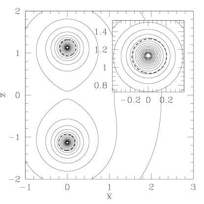
FIG. 2.: Contours of the conformal factor $\psi$ for a configuration close to the innermost stable circular orbit ($\bar{C}=2.25$ and $\bar{J}=2.95$). The contours (solid lines) logarithmically span the interval $\psi=1$ and $\psi=9.2$. Note that the apparent horizons, marked by the thick dashed lines, are not concentric with the contours of the conformal factor. Instead, they are dragged along by the black holes and lag slightly behind in their (counter-clockwise) orbit.

In Fig. 2, we show contour plots of the conformal factor $\psi$ for a configuration close to the ISCO ($\bar{C}=2.25$ and $\bar{J}=2.95$). The apparent horizons, marked by the thick dashed lines, are dragged along by the black holes and lag slightly behind in their counter-clockwise orbit. This effect has been discussed for single boosted black holes in [34]. Note that we compute the proper separation $\bar{l}\equiv l/m$ between the horizons along the line connecting the centers of the apparent horizons. This is a coordinate-dependent quantity, but a very good approximation to the (coordinate-independent) shortest proper separation between the horizons.

We now construct sequences of constant angular momentum for various values of $\bar{J}$, and plot the effective potential $\bar{E}_{b}$ along these sequences as a function of $\bar{l}$ in Fig. 3. A minimum in the effective potential corresponds to a stable quasicircular orbit. The bold line connecting these minima in Fig. 3 represents a sequence of quasicircular orbits. This sequence terminates at the ISCO, where the adiabatic, quasicircular inspiral of the two black holes is expected to change into a rapid plunge and merger [2]. Since this transition leaves a characteristic signature in the gravitational wave signal, the knowledge of the location and frequency of the ISCO are of great importance for future observations with the new generation of gravitational wave detectors.

FIG. 3.: The effective potential $\bar{E}_{b}$ as a function of proper separation $\bar{l}$ for the following values of the angular momentum $\bar{J}$: 2.9, 2.92, 2.94, 2.95, 2.96, 2.97, 2.98, 3.00, 3.02, 3.06, 3.10, 3.15, 3.20, 3.25 (from bottom to top). Quasicircular orbits correspond to minima in the effective potential. The bold line connects these minima and represents a sequence of quasicircular orbits. This sequence terminates at the innermost stable circular orbit.

$\bar{l}$	$\bar{E}_{b}$	$\bar{J}$	$\bar{\Omega}$	$P/a$	$C/a$
4.8	-0.092	2.95	0.18	1.7	5.9
4.880	-0.09030	2.976	0.172	1.685	5.91

TABLE I.: Comparison of our results for the innermost stable circular orbit (top line) with those of Cook [10] (bottom line).

In Table I, we list our results for the physical parameters of the ISCO (top line) and compare with the results of Cook [10] (bottom line). We tabulate the proper separation between the horizons $\bar{l}$, the binding energy $\bar{E}_{b}$, the angular momentum $\bar{J}$, and the angular velocity $\bar{\Omega}$ as well as the the linear momentum of each black hole $P/a$ and the coordinate separation $C/a$, where $a$ is the (coordinate) radius of the black holes. The latter is not well-defined in our calculation, but since the black holes are nearly spherical it is very reasonable to estimate an average radius from the $\ell=0$ monopole term in the multipole expansion for the horizon.

We conclude that all quantities agree fairly well with those of Cook [10] within our estimated numerical error of a few percent. As the most significant deviation, we find that in our calculation the binary is slightly more tightly bound at the ISCO, and correspondingly has a slightly larger angular velocity. However, even these quantities differ by less than $\sim 5\%$, which may be caused by numerical effects. We conclude that the choice of the underlying manifold structure has a very small effect on the location of the ISCO.

Reference	$\bar{E}_{b}$	$\bar{J}$	$\bar{\Omega}$
Schwarzschild	-0.0572	3.464	0.068
CE [5]	-0.1	3.3	—
BD [6]	-0.65	0.85	2
KWW [7]	-0.0378	3.83	0.0605
Cook [10]	-0.09030	2.976	0.172
BCSST [11]	-0.048	3.9	0.06
DIS [8]	-0.0653	—	0.0885
BD [9]	-0.06005	3.40	0.0734
This work	-0.092	2.95	0.18

TABLE II.: Comparison of the binding energy $\bar{E}_{b}$, the angular momentum $\bar{J}$ and the angular velocity $\bar{\Omega}$ for the innermost stable circular orbit from various different calculations: a test particle orbiting a Schwarzschild black hole, Clark and Eardley (CE) [5], Blackburn and Detweiler (BD) [6], Kidder, Will and Wiseman (KWW) [7], Cook [10], Baumgarte et.al. (BCSST) [11], Damour, Iyer and Sathyaprakash (DIS) [8], Buonanno and Damour (BD) [9], and the results from this paper. The results of Baumgarte et.al. [11] are for an $n=1$ polytrope binary of compaction $M/R=0.2$. Naively extrapolating to $M/R=0.5$ yields values very close to our results for binary black holes.

In Table II we compare the binding energy, the angular momentum and the angular velocity at the ISCO from various different calculations. For a test particle orbiting a Schwarzschild black hole, the ISCO can be located analytically, which yields $\bar{E}_{b}=\sqrt{8/9}-1\sim-0.0572$, $\bar{J}=2\sqrt{3}\sim 3.464$, and $\bar{\Omega}=1/6^{3/2}\sim 0.0680$. Clark and Eardley [5] adopted a first order post-Newtonian argument to approximately estimate the location of the ISCO. We list their values for nonrotating neutron stars. Blackburn and Detweiler [6] adopted a variational principle and assumed a periodic solution to Einstein’s equations. At the ISCO, for which the approximations of this approach fail, they find extremely tightly bound binaries. Kidder, Will and Wiseman [7] adopted a second order post-Newtonian approximation together with a “hybrid” approach and found an extremely weakly bound ISCO. However, several authors have cast doubt on the robustness and consistency of the hybrid approach [35, 8]. Baumgarte et.al. [11] constructed fully relativistic models of corotating binary neutron star in quasiequilibrium, albeit assuming conformal flatness, and found that the ISCO depends on the compaction of the neutron stars. In Table I we list their results for $n=1$ polytropes of compaction $M/R=0.2$, where $M$ and $R$ are the mass-energy and areal radius which the stars would have in isolation. Naively extrapolating their results to $M/R=0.5$ yields values which are very similar to our result for binary black holes. Damour, Iyer and Sathyaprakash [8] combined a second order post-Newtonian approximation with a Padé approximation, which yields a slightly more tightly bound ISCO than that for a test-particle orbiting a Schwarzschild black hole. A similar result is found by Buonanno and Damour, who combine a second order post-Newtonian approximation with an effective-one-body method [9, 3].

V SUMMARY AND DISCUSSION

Since an accurate knowledge of the ISCO is very important for possible future gravitational wave observations, it is very unsettling that different approaches to computing the ISCO lead to very different results (compare Table II). One of these approaches, namely constructing binary black hole solutions to the constraint equations of general relativity, involves choosing the background geometry and topology, and it would be very desirable to know how much the results depend on these choices.

In this paper, we introduce a new method to construct solutions to the constraint equations of general relativity describing binary black holes in quasicircular orbit. We combine the approaches of Cook [10] and Brandt and Brügmann [12] to construct binary black holes in a three-sheeted manifold structure, as opposed to the two-sheeted topology in the conformal-imaging approach adopted by Cook [10]. We locate the ISCO and find that its physical parameters are very similar to those found by Cook [10]. Our results confirm those earlier results and imply that the underlying manifold structure only has a very small effect on the ISCO. The latter is perhaps not entirely surprising, since it reflects the fact that the strength of the imaged poles in the conformal-imaging approach is smaller than the strength of the poles themselves [20].

Our new approach is considerably simpler than the conformal-imaging approach of Cook [10]. The analytic solution to the momentum constraint simplifies because no inversion-symmetric solutions have to be constructed, and the numerical solution to the Hamiltonian constraint simplifies because we can adopt the “puncture” method of Brandt and Brügmann [12]. In particular, we can solve the Hamiltonian constraint in cartesian coordinates on $R^{3}$ without having to impose interior boundary conditions. One disadvantage of our approach is that the apparent horizons have to be located numerically, which we do with the algorithm developed in [32].

In this paper, we follow Cook [10] and choose a conformally flat background metric. Accordingly, we cannot address the dependence of the ISCO on the choice of the background geometry. However, since our new method is significantly simpler than the conformal-imaging approach, it may provide a useful framework to relax the assumption of conformal flatness and to construct binary black holes in quasicircular orbit for more general background geometries.

- [1] See, e.g., the talks presented at the ITP Miniprogram Colliding Black Holes: Mathematical Issues in Numerical Relativity (doug-pc.itp.ucsb.edu/online/numrel00/).
- [2] Note that the transition from adiabatic inspiral to dynamical plunge at the innermost stable circular orbit may be fairly gradual [3, 4].
- [3] A. Buananno and T. Damour, submitted (2000), also gr-qc/0001013.
- [4] A. Ori and K. S. Thorne, submitted (2000), also gr-qc/0003032.
- [5] J. P. A Clark and D. M. Eardley, Astrophys. J. 215, 311 (1977).
- [6] J. K. Blackburn and S. Detweiler, Phys. Rev. D 46, 2318 (1992).
- [7] L. E. Kidder, C. M. Will and A. G. Wiseman, Class. Quantum Grav. 9, L125 (1992); Phys. Rev. D 47, 3281 (1993).
- [8] T. Damour, B. R. Iyer and B. S Sathyaprakash, Phys. Rev. D 57, 885 (1998).
- [9] A. Buananno and T. Damour, Phys. Rev. D 59, 084006 (1999).
- [10] G. B. Cook, Phys. Rev. D 50, 5025 (1994).
- [11] T. W. Baumgarte, G. B. Cook, M. A. Scheel, S. L. Shapiro, and S. A. Teukolsky, Phys. Rev. Lett. 79, 1182 (1997); Phys. Rev. D 57, 7292 (1998).
- [12] S. Brandt and B. Brügmann, Phys. Rev. Lett. 78, 3606 (1997).
- [13] R. Arnowitt, S. Deser and C. W. Misner, in Gravitation: An Introduction to Current Research, edited by L. Witten (Wiley, New York, 1962).
- [14] J. W. York, Jr., Phys. Rev. Lett. 26, 1656 (1971).
- [15] J. W. York, Jr., in Sources of Gravitational Radiation, edited by L. L. Smarr (Cambridge University Press, Cambridge, England, 1979).
- [16] G. B. Cook, Phys. Rev. D 44, 2983 (1991).
- [17] G. B. Cook, M. W. Choptuik, M. R. Dubal, S. Klasky, R. A. Matzner and S. R. Oliveira, Phys. Rev. D 47, 1471 (1993).
- [18] A. Einstein and N. Rosen, Phys. Rev. 48, 73 (1935).
- [19] R. W. Linquist, J. Math. Phys. 4, 938 (1963).
- [20] C. W. Misner, Ann. Phys. (N.Y.) 24, 102 (1963).
- [21] A. D. Kulkarni, L. C. Shepley and J. W. York, Jr., Phys. Lett. 96A, 228 (1983).
- [22] A. Čadež, Ph.D. dissertation, University of North Carolina (1971); see also Appendix C in [16].
- [23] Note that these integrals are in terms of cartesian coordinates.
- [24] J. Bowen and J. W. York, Jr., Phys. Rev. D 21, 2047 (1980).
- [25] J. Bowen, Gen. Relativ. Gravit. 11, 227 (1979).
- [26] J. W. York, Jr., in Frontiers in Numerical Relativity, edited by C. R. Evans, L. S. Finn, and D. W. Hobbill (Cambridge University Press, Cambridge, 1989).
- [27] C. Christodoulou, Phys. Rev. Lett. 25, 1596 (1970).
- [28] To illustrate this approach, consider two Newtonian point-masses of mass at a separation , for which . Minimizing for constant and yields for circular orbits. The orbital angular velocity can then be found from , where the derivative is taken for constant and . Combining the two results recovers, as expected, the Kepler law .
- [29] M. Parashar and J. C. Brown, in Proceedings of the International Conference for High Performance Computing, edited by S. Sahni, V. K. Prasanna and V. P. Bhatkar (Tata McGraw-Hill, New York, 1995), also www.caip.rutgers.edu/parashar/DAGH/.
- [30] S. Balay, W. D. Gropp, L. C. McInnes, and B. F. Smith, in Modern Software Tools in Scientific Computing, edited by E. Arge, A. M. Bruaset and H. P. Langtangen, p. 163, Birkhauser Press, 1997; see also the PETSc home page http://www.mcs.anl.gov/petsc.
- [31] B. Brügmann, private communication.
- [32] T. W. Baumgarte, G. B. Cook, M. A. Scheel, S. L. Shapiro, and S. A. Teukolsky, Phys. Rev. D 54, 4849 (1996).
- [33] Alternatively, all quantities could be rescaled with respect to the numerical values of . In this case, no iteration is needed to achieve , since this obviously holds identically, but instead an iteration is necessary to find a desired value of (see [10]).
- [34] G. B. Cook and J. W. York, Jr., Phys. Rev. D 41, 1077 (1990).
- [35] N. Wex and G. Schäfer, Class. Quantum Grav. 10, 2729 (1993); also G. Schäfer and N. Wex, in XIIIth Moriond Workshop: Perspectives in Neutrinos, Atomic Physics and Gravitation, edited by J. Trân Thanh Vân, T. Damour, E. Hinds and J. Wilkerson (Editions Frontières, Gif-sur-Yvette, 1993), p. 513.