The general treatment of high/low energy particle
interference phase in a gravitational field

Abstract

The interference phase of the high/low energy particle in a gravitational field is studied. By means of the complete Schwarzshild tetrads, we again deal with the phase in terms of the type-I and type-II phases, which correspond to the momentum and “spin connection” of Dirac particle coupling to the curved spacetime respectively. We find that the type-II phase is in the magnitude of the square of the gravitational potential, which can be neglected in the weak field. For the high energy particle (mass neutrinos), we obtain that the phase calculated along the null is equivalent to the half phase along the geodesic in the high energy limit. Further, we apply the covariant phase to the thermal neutron interference, and obtain the consistent interference phase with that exploited in COW experiment.

PACS number(s): 95.30.Sf, 26.30.+k, 14.60.Pq

I Introduction

The neutrino oscillations have been a hot topic in the high energy experimental and theoretical phycics recently [1, 2], in particular, with highly confident atomspheric neutrino experiment of Super-Kamiokande to assure the neutrino mass  [3]. As a natural extension of the theoretical consideration, the description of neutrino oscillation in the flat spacetime should be replaced by that in the curved spacetime if the gravitational background is taken into account. In other words, the physics related to the neutrino oscillation in Minkowski spacetime with Lorentz invariant will be extended to Riemanian spacetime with general coordinate transformation. The pioneer theoretical considerations on the gravitationally induced neutrino oscillation were proposed by Wudka [4], and later advocated by Ahluwalia [5] who for the first time presented the three flavor neutrino oscillations in the weak field expansion scheme. Further some thoughtful idea on the nongeometrical element in the description of the gravitational theory, trigered by the gravitationally induced neutrino oscillation clock, was also provided [5]. Moreover the violation of the equivalence principle was also employed to account for the significant influence on the MSW effect [6] for the solar neutrinos [7, 8]. More recently, from the different angle, the gravitational effects on the neutrino oscillations have been paid much attention by a number of authors [5, 9, 10, 11, 12, 13], but, unfortunately, debates and conflicts occur in the understanding of the gravitationally induced neutrino oscillations  [5, 10, 11, 12, 13].

In this paper, we will discuss the particle interference phase in a gravitational field in a unified version, i.e., provide a unified description of the phases for both high energy particle (two mass neutrinos) and low energy particle (COW thermal neutrons). In order to develope the treatments by using the null condition to calculate the neutrino relative phase and appling the weak field condition to calculate COW thermal neutron phase, we employ the accurate particle world line (geodesic) to calculate both phase factors, and at last we can obtain the correct neutrino relative phase by dividing a factor of 2 and obtain the COW neutron interference phase by the convenient approximated condition.

The energy condition in the gravitational field to account for the relative phase of mass neutrinos often makes the confusions and even conflicts[5, 11, 12]. Apparently, we point out that almost all debates related to the neutrino oscillation in curved spacetime originate from the inconvenient use of this condition. It is noted that replacing the null by the geodesic to calculate the neutrino oscillation phase will produce a factor of 2 error. However this factor of 2 will be automatically deleted when considering the two neutrino arrival time differnce[12]. Here, we still follow the plane wave treatment for the extremely relativistic neutrinos in the framework of the standard treatment [13], otherwise the wave packet treatment will be applied for the general case [14].

For the reason of simplicity, we confine our treatment in two generation neutrinos (electron and muon) and mainly in Schwarzschild geometry with radial propagation and nonradial propagation respectively. The purpose of the paper is threefold. First we point out the general treatment of the high (low) energy particle phase in a gravitational field, include the type-I and type-II phases. Second we give the complete description of neutrino phase along the geodesic, and point out the relation to that by the null in the high energy limit. Third we apply the covariant geodesic phase to the COW thermal interference phase, then we can find that the geodesic phase can result in the correct results for the interference phases of both the two mass neutrinos and the thermal neutron by the standard treatment.

So the paper is organized as follows. In Sec. II, we discuss Dirac equation and the treatments of particle interference phase in the curved spacetime, which includes type-I and type-II phases. In Sec. III and Sec. IV, we calculate the neutrino oscillation phase in Schwarzschild spacetime along the geodesic, and compare it with that along the null, in the radial and nonradial directions respectively. The application of the unified geodesic phase to the COW thermal neutron interference is done in Sec. V. Furthermore, discussions and conclusions involved in the high energy neutrino oscillations and low energy thermal neutron interference in curved spacetime are given. We set $G=\hbar=c=1$ throughout this article.

II Dirac equation in a curved spacetime

Previous to entering our main point, we stress that the semiclassical approximated Dirac particle does not follow the geodesic exactly, but the force aroused by the spin and the curvature coupling has a little contribution to the geodesic deviation [15]. So here we take the neutrino as a spinless particle to go along the geodesic [4]. The gravitational effects on the spin incorporated into Dirac equation through the “spin connection” $\Gamma_{\mu}$ appearing in the Dirac equation in curved spacetime [16, 17], which is constructed by means of the variation of the covariant Lagrangian of the spinor field as,

$$\left[\gamma^{a}h^{\mu}_{a}(\partial_{\mu}+\Gamma_{\mu})+m\right]\psi=0.$$ (1)

In this equation and in the rest of this section, greek indices $\mu,\nu,\sigma$ refer to general covariant (Riemanian) coordinates, while the latin indices $a,b,c,d$ refer to locally Lorentz (Minkowski) coordinates. The tetrads $h_{a}{}^{\mu}$ connect these sets of coordinates by

$$g_{\mu\nu}=\eta_{ab}\;h^{a}{}_{\mu}\;h^{b}{}_{\nu}\;,$$ (2)

the tetrads are supposed to satisfy the following relation

$$h^{a}{}_{\mu}\;h_{a}{}^{\nu}=\delta_{\mu}{}^{\nu}\quad;\quad h^{a}{}_{\mu}\;h_{b}{}^{\mu}=\delta^{a}{}_{b}\;.$$ (3)

The explicit expression for $\Gamma_{\mu}$ can be written in terms of the Dirac matrices and tetrads(see  [11])

$$\Gamma_{\mu}={1\over 8}[\gamma^{b},\gamma^{c}]h_{b}{}^{\nu}h_{c\nu;\mu}.$$ (4)

We must first simplify the Dirac matrix product in the spin connection term. It can be shown that

$$\gamma^{a}[\gamma^{b},\gamma^{c}]=2\eta^{ab}\gamma^{c}-2\eta^{ac}\gamma^{b}-2i\epsilon^{dabc}\gamma_{5}\gamma_{d},$$ (5)

where $\eta^{ab}$ is the metric in flat space and $\epsilon^{abcd}$ is the (flat space) totally antisymmetric tensor, with $\epsilon^{0123}=+1$. With Eq.(5), the contribution from the spin connection is arranged as

$$\Gamma_{\mu}={1\over 2}v_{\mu}-{3i\over 4}a_{\mu}\gamma_{5},$$ (6)

where $v_{\mu}$ is the tetrad vector and $a_{\mu}$ is the tetrad axial-vector respectively, defined by

$$v_{\mu}=T^{\lambda}{}_{\lambda\mu},\,\,\,a_{\mu}={1\over 6}\epsilon_{\mu\nu\lambda\sigma}T^{\nu\lambda\sigma}$$ (7)

$$T^{\sigma}{}_{\mu\nu}=\Gamma^{\sigma}{}_{\nu\mu}-\Gamma^{\sigma}{}_{\mu\nu}\;\;,\;\;\Gamma^{\sigma}{}_{\mu\nu}=h_{a}{}^{\sigma}\partial_{\nu}h^{a}{}_{\mu}\;,$$ (8)

If $v_{\mu}\rightarrow 0$, then the expression of Eq.(6) is recovered to the form obtained by Cardal and Fuller [11]. It is instructive to outline the properties of the spin connection. We can see that the two terms in the spin connection represent the different aspects of the gravitational coupling with the Dirac field. The second term of r.h.s. of Eq.(6), proportional to $i\gamma_{5}$, has the similar form to the weak interaction field [18, 19]. Moreover $a^{\mu}$ is an axial-vector, which represents the physical modification from axial symmetry to the spherical symmetry [21]. From the gravitational interation point of view, $a^{\mu}$ shows the rotational gravitational field property, or the angular momentum aspect of gravitational field, in other words, it represents the gravitomagnetic like interaction. However the first term of Eq.(6) is similar to the canonical momentum, then its contribution seems to be the gravitational field momentum. In order to group Eq.(6) with terms arising from the matter effects, we can without physical consequence arrange Eq.(6) as follows

$$\Gamma_{\mu}=P_{G\mu}+iA_{G\mu}{\cal P}_{L},$$ (9)

$$A^{\mu}_{G}\equiv{h\over 4}h_{a}{}^{\mu}\epsilon^{abcd}(h_{b\nu,\sigma}-h_{b\sigma,\nu})h_{c}{}^{\nu}h_{d}{}^{\sigma}={3h\over 2}a^{\mu},$$ (10)

$$P_{G\mu}={1\over 2}v_{\mu}\;\;,\;\;{\cal P}_{L}=\left[-{\gamma_{5}\over 2h}\right].$$ (11)

In these equations, $h=(-g)^{1/2}=[\rm det(g_{\mu\nu})]^{1/2}$. The expression in Eq.(9) treats left- and right-handed states differently. Proceeding as in the discussion of matter effects, we will borrow the neutrino oscillation standard treatment in a gravitational field in  [11], where the gravitational induced effective mass can be calculated from the mass shell condition, which is obtained by iterating the Dirac equation

$$(P_{\mu}+P_{G\mu}+A_{G\mu}{\cal P}_{L})(P^{\mu}+P_{G}^{\mu}+A_{G}^{\mu}{\cal P}_{L})=m^{2},$$ (12)

where $P_{\mu}$ is the 4-momentum, and we have not included background matter effects. However, the following approximated conditions are usually valid for neutrinos, i.e., $P_{\mu}>>P_{G\mu}$, $P_{\mu}>>A_{G\mu}$ and $P_{\mu}>>m$.

The complication in calculating the neutrino phase in curved spacetime is related to the nature of the neutrino trajectories. In flat spacetime, the neutrino trajectories are straight lines. But in the curved spacetime, the geodesic is curved from the global point of view, which is more complicated than the situation of the flat spacetime. Now we will follow the factual mass particle world line to cope with the neutrino oscillation problem, but we can prove that the neutrino phase along the null is the half of the value along the geodesic in the high energy limit (see APPENDIX A). However the relative phase of two mass neutrinos should be equivalent to that along the geodesic through dividing a factor of 2 because the arrival time difference of two mass neutrinos should be considered[12].

In flat spacetime, the phase factor can be written as a conventional manner [11, 17, 20],

$${\Phi}=\int mds=\int(Edt-Pdx)=\int\eta_{\mu\nu}P^{\mu}dx^{\nu},$$ (13)

where phase factor $\Phi$ is also the classical Langrange for the particle motion, and the route is along the particle world line(geodesic) determined by the variational principle or Jacobi-Hamilton equation [9, 15, 17]. ds is the interval in flat spacetime with $ds^{2}=\eta_{\mu\nu}dx^{\mu}dx^{\nu}$ and the metric $\eta_{\mu\nu}=diag(+1,-1,-1,-1)$. In the curved spacetime, however, the neutrino phase is calculated along the null[11, 13]

$${\Phi}=\int md\lambda=\int g_{\mu\nu}P^{\mu}dx^{\nu}=\int P_{\mu}\stackrel{{\scriptstyle\circ}}{{n}}{}^{\mu}d\lambda,$$ (14)

where $\lambda$ is the affine parameter along the null. For the null (photon trajectory) it therefore may be convenient to leave the affine parameter $\lambda$ as the variable of integration in Eq.(14). The tangent vector to the null ${\stackrel{{\scriptstyle\circ}}{{n}}}{}^{\mu}=dx^{\mu}/d\lambda$, and ${x^{\mu}}(\lambda)=\left[x^{0}(\lambda),x^{1}(\lambda),x^{2}(\lambda),x^{3}(\lambda)\right]$. Now we consider the general mass shell condition and ignore the terms of ${\cal O}(A^{2})$, ${\cal O}(AM)$, ${\cal O}(P_{G\mu}^{2})$ and ${\cal O}(P_{G\mu}M)$. Following ref.[11], we obtain

$$P_{\mu}\stackrel{{\scriptstyle\circ}}{{n}}{}^{\mu}=m^{2}/2P_{o}-A_{G\mu}\stackrel{{\scriptstyle\circ}}{{n}}{}^{\mu}-P_{G\mu}\stackrel{{\scriptstyle\circ}}{{n}}{}^{\mu}.$$ (15)

From Eq.(15), we find that the total phase includes two types. The first type is contributed by the phase of the spinless particle $m^{2}/2P_{o}$, which is conventionally discussed [11, 13] and the second type is contributed by the “spin connection”. According to the definition by Anandan [17], the type-I phase represents the contribution of the particle momentum coupled to the spacetime cuvature, and the type-II phase represents the spin connection contribution of the particle coupled to the spacetime geometry.

Further, it is convenient to define a column vector of flavor amplitudes [11]. For example, for mixing between $\nu_{e}$ and $\nu_{\tau}$,

$$\chi(\lambda)\equiv\pmatrix{\langle\nu_{e}|\Psi(\lambda)\rangle\cr\langle\nu_{\tau}|\Psi(\lambda)\rangle}.$$ (16)

Eq.(16) can be written as a differential equation for the null parameter $\lambda$,

$$i{d\chi\over d\lambda}=\left(m^{2}/2P_{o}-A_{G\mu}\stackrel{{\scriptstyle\circ}}{{n}}{}^{\mu}-P_{G\mu}\stackrel{{\scriptstyle\circ}}{{n}}{}^{\mu}\right)\chi,$$ (17)

Eq.(17) can be integrated to yield the neutrino flavor evolution. A similar equation was obtained in Ref. [11].

III Radial neutrino oscillation in Schwarzschild spacetime

In this section we will study the phases along the geodesic and along the null in Schwarzschild spacetime. In Schwarzshild geometry, the spherically static spacetime can be globally represented by the Schwarzshild coordinate system $\{x^{\mu}\}=(t,r,\theta,\phi)$ with the line element as

$$ds^{2}=g_{oo}dt^{2}+g_{11}dt^{2}-r^{2}d\theta^{2}-r^{2}sin^{2}\theta d\phi^{2},$$ (18)

$$g_{oo}=(-g_{11})^{-1}=1-{r_{s}\over r},$$ (19)

where $r_{s}=2M$ is Schwarzschild radius and M is the gravitational mass of star. The general form of tetrads in Schwarzshild spacetime are given as follows (see APPENDIX B). The spacelike components of coordinates share the SO(3) rotational symmetry and timelike coordinate shares the reflection symmetry

$$h^{a}{}_{\mu}\equiv\pmatrix{\gamma_{oo}&0&0&0\cr 0&\gamma_{11}s\theta c\phi&r\;c\theta c\phi&-r\;s\theta s\phi\cr 0&\gamma_{11}s\theta s\phi&r\;c\theta s\phi&r\;s\theta c\phi\cr 0&\gamma_{11}c\theta&-r\;s\theta&0}$$ (20)

where $\gamma_{oo}=\sqrt{g_{oo}}$, $\gamma_{11}=\sqrt{-g_{11}}$, $s=\sin$ and $c=\cos$, and the subscript $\mu$ is the column index. This tetrad deduces the tetrad axial vector and tetrad vector $a^{\mu}=0$ and $v^{\mu}=(0,v^{1},0,0)$. It is easy to understand that the axial tetrad is cancelled in the case of the spherical symmetry, which represents the deviation from the spherical symmetry and occurs in the Kerr spacetime [21]. The nonzero tetrad vector(see APPENDIX B)

$$v_{1} = g_{11}v^{1}=-(g_{oo})^{-1}\left[[ln\sqrt{g_{oo}}]^{{}^{\prime}}+{1-\sqrt{g_{11}}\over r}\right]$$ (21)

$$= {1\over 2}(-g_{11})^{{}^{\prime}}+{g_{11}\over r}(1-\sqrt{-g_{11}}),$$ (22)

so the type-II phase is

$$\Phi_{II} = \int P_{G\mu}dx^{\mu}=\int_{r_{o}}^{r}v_{1}/2dr$$ (23)

$$= {1\over 4}\left[r-r_{o}+ln{(1-{r_{s}\over r})\over(1-{r_{s}\over r_{o}})}\right]$$ (24)

$$\simeq {-1\over 8}\left[({r_{s}\over r})^{2}-({r_{s}\over r_{o}})^{2}\right].$$ (25)

From Eq.(25), if $r\rightarrow r_{s}$, the type-II phase will be infinite. Then in the weak field, we can conclude that the type-II phase for neutrino in the curved spacetime is proportional to the square of the gravitational potential, i.e., $({r_{s}\over 2r})^{2}$, which is lower than the contribution of the type-I phase that is related to the gravitational potential, i.e., the gravitational red shift [11, 13]. But, if we consider the strong gravitational field, e.g., near the horizon of the black hole[9], the type-II phase might produce some effects on the particle interference. However, we stress that the type-II phase of Eq.(25) is independent of the neutrino mass, namely it is equally contributed to the different neutrinos. So this leads to the cancelling of the relative type-II phase between the different mass neutrinos. Therefore we only consider the type-I phase of the mass neutrinos in the Schwarzschild geometry by means of the particle geodesic equation

$${d^{2}x^{\lambda}\over ds^{2}}+{\stackrel{{\scriptstyle\circ}}{{\Gamma}}}{}^{\lambda}_{\mu\nu}{dx^{\mu}\over ds}{dx^{\nu}\over ds}=0$$ (26)

where

$${\stackrel{{\scriptstyle\circ}}{{\Gamma}}}{}^{\lambda}{}_{\mu\nu}=\frac{1}{2}g^{\lambda\rho}\left[\partial_{\mu}g_{\rho\nu}+\partial_{\nu}g_{\rho\mu}-\partial_{\rho}g_{\mu\nu}\right]$$ (27)

is the Levi–Civita connection. Along radial direction with $d\theta=d\phi=0$, there are two nontrivial independent equations in the four geodesic equations(see Appendix C). The nontrivial equation of timelike

$$\ddot{t}+{\dot{g_{oo}}\over g_{oo}}\dot{t}=0$$ (28)

where the dot represents the derivative to ds, for instance, $\dot{t}={dt\over ds}$. The Eq.(28) gives

$$g_{oo}\dot{t}=const.,~{}~{}~{}or,~{}~{}~{}E=P_{o}=mg_{oo}\dot{t}=const.$$ (29)

Eq.(29) represents that the covariant energy is the motion constant along the geodesic, by which the calculation of the phase is proceeded. It is stressed that it is the covariant energy $P_{o}$ (not $P^{o}$) the constant of motion, then this fact will be important in the later calculation of the neutrino phase. Otherwise the ambiguous definition of the neutrino energy in the gravitational field will lead to the confusion in understanding the gravitationally induced neutrino oscillation.

The mass shell condition can be written in the Schwarzshild spacetime, which is not independent and can be deducted from the geodesic equations

$$g_{oo}\dot{t}^{2}+g_{11}\dot{r}^{2}+r^{2}\dot{\phi}^{2}=1,~{}~{}~{}$$ (30)

substituting Eq.(29) into Eq.(30) with $\dot{\phi}=0$, which means the radial motion, thus we obtain

$${ds\over dr}=\sqrt{{-g_{oo}g_{11}\over({P_{o}\over m})^{2}-g_{oo}}}.$$ (31)

If $m\rightarrow 0$, then ${ds\over dr}=0$, the null condition is recovered. If $r\rightarrow\infty$, the asympotic flat solution $g_{oo}\rightarrow 1$ and $-g_{11}\rightarrow 1$ is obtained, by which we can acquire the phase of flat spacetime. In Schwarzshild spacetime, $-g_{oo}g_{11}=1$, Eq.(31) becomes simply

$${ds\over dr}={1\over\sqrt{({P_{o}\over m})^{2}-g_{oo}}}=({m\over P_{o}})(1+\delta^{2}).$$ (32)

where $\delta^{2}={g_{oo}\over 2}({m\over P_{o}})^{2}$. The accurate phase factor in Schwarzshild spacetime along the radial direction is acquired in virtue of the phase factor

$$\Phi(geod) = \int m({ds\over dr})dr=\int{mdr\over\sqrt{({P_{o}\over m})^{2}-g_{oo}}}$$ (33)

$$= ({mr\over k})\sqrt{k+{r_{s}\over r}}-({mr_{o}\over k})\sqrt{k+{r_{s}\over r_{o}}}$$ (34)

$$- ({mr_{s}\over 2k^{3/2}})log\left[r_{s}+2kr+2r\sqrt{k(k+{r_{s}\over r})}\right]$$ (35)

$$+ ({mr_{s}\over 2k^{3/2}})log\left[r_{s}+2kr_{o}+2r_{o}\sqrt{k(k+{r_{s}\over r_{o}})}\right]$$ (36)

$$\approx {m^{2}\over P_{o}}(r-r_{o})+O(\delta^{2})=2\Phi(null),$$ (37)

where $k=({P_{o}\over m})^{2}-1$. $\Phi(null)={m^{2}\over 2P_{o}}(r-r_{o})$ is the neutrino phase along the null given by  [11, 13].

It is noted that the Schwarzschild coordinates r and $r_{o}$ are not the applicable physical distances, and the physical distance connected coordinate is given by $dL=\sqrt{-g_{11}}dr$, where dL is the physical distance. The quantity $0\leq g_{oo}\leq 1$ leads to $g_{oo}\ll k\sim 10^{12}$ for the electron neutrino. In other words, the gravitational contribution appears in one part of $10^{12}$ as shown in Ref. [12]. This means that the Schwarzschild gravitation has little contribution to the neutrino oscillation phase, which is same as that concluded in  [11, 12]. The above phase calculation is a precisely treatment, and we do not use any approxamations, except the final approximated simplification. However, we admit that the Schwarzschild coordinates employed to calculate the phase factor is not the real physical distance although there exists some complications between them in the general case.

In order to illustrate the validity of the geodesic phase treatment, we calculate the geodesic phase again from the other method. From the equations (30) and (32), the derivative between the time-like and the space-like coordinates,

$${dt\over dr} = \sqrt{{(-g_{11})\over g_{oo}}}[1-({m\over P_{o}})^{2}g_{oo}]^{-1/2}$$ (38)

$$\approx \sqrt{{(-g_{11})\over g_{oo}}}(1+\delta^{2}),\,\,\,$$ (39)

If the neutrino mass $m\rightarrow 0$, then $\delta\rightarrow 0$, which leads to the null condition ${dt\over dr}=\sqrt{{(-g_{11})\over g_{oo}}}$ that is conventionally used in the standard treatment[11, 13]. For the electron neutrino, the mass $m\sim 1$ ev and the energy $E\sim 1$ Mev, $\delta^{2}\sim 10^{-12}$[18, 19], which is really a little quantity. If we set $\delta=0$, then Eq.(38) represents the null condition, which will produce the null phase [11, 13]. But, if this almost negligible quantity is taken into account, then what do the things occur to the phase calculation? Let us follow the very routine phase calculation as proceeded in the standard treatment of the neutrino phase in a gravitational field,

$$\Phi=\int g_{\mu\nu}P^{\mu}dx^{\nu}\\ =\int(g_{oo}P^{o}dt+g_{11}P^{r}dr).$$ (40)

The mass shell condition in Schwarzshild spacetime

$$g_{\mu\nu}P^{\mu}P^{\nu}=m^{2},\,\,\,g_{oo}(P^{o})^{2}+g_{11}(P^{r})^{2}=m^{2},$$ (41)

and the approximated energy momentum relation from Eq.(41)

$$(-g_{11})P^{r}=\sqrt{g_{oo}(-g_{11})}P^{o}-\sqrt{{(-g_{11})\over g_{oo}}}{m^{2}\over 2P^{o}},$$ (42)

substituting (42) and (38) into (40), we obtain

$$\Phi(geod) = \int\left[g_{oo}P^{o}{dt\over dr}+g_{11}P^{r}\right]dr$$ (43)

$$= \int\left[\sqrt{{(-g_{11})g_{oo}}}P^{o}\delta^{2}+\sqrt{{(-g_{11})g_{oo}}}{m^{2}\over 2P_{o}}\right]dr$$ (44)

$$= \int\left[\sqrt{{(-g_{11})g_{oo}}}{m^{2}\over 2P_{o}}+\sqrt{{(-g_{11})g_{oo}}}{m^{2}\over 2P_{o}}\right]dr$$ (45)

$$= \int\sqrt{{(-g_{11})g_{oo}}}({m^{2}\over P_{o}})dr$$ (46)

$$= {m^{2}\over P_{o}}(r-r_{o})+O(\delta^{2})=2\Phi(null).$$ (47)

It is not strange that the geodesic phase is double of the result by the null [11]. This also indicates that the application of the null condition arises the correct result, and the geodesic phase of two neutrinos despises the two neutrino arrival time difference[12].

Now we discuss the physical coordinate problem because the Schwarzschild coordinate employed in Eq.(43) is not the proper physical distance, however, which is given by

$$L-L_{o}\hbox{} \hbox{}\equiv\hbox{} \hbox{}\int_{r_{o}}^{r}\sqrt{-g_{11}}\,dr$$ (48)

$$\hbox{}=\hbox{} \hbox{}r\sqrt{1-{r_{s}\over r}}-r_{o}\sqrt{1-{r_{s}\over r_{o}}}$$ (49)

$$+ r_{s}\left[\ln\!\left(\sqrt{r-r_{s}}+\sqrt{r}\right)-\ln\!\left(\sqrt{r_{o}-r_{s}}+\sqrt{r_{o}}\right)\right]\;.$$ (50)

We consider the case of a weak field, then the physical distance is approximately obtained

$$L-L_{o}\simeq r-r_{o}+{r_{s}\over 2}\ln\frac{r}{r_{o}}\;,$$ (51)

where L($L_{o}$) is the proper physical distance corresponding to the coordinate r ($r_{o}$). In the case of weak field as well as the conditions $\Delta L=L-L_{o}\ll L$ and $\Delta r=r-r_{o}\ll r$, we obtain

$$\Delta r=(1-{r_{s}\over 2L})\Delta L=\left[1+V(L)\right]\Delta L\;,$$ (52)

where $V(L)={-r_{s}\over 2L}$ is the gravitational potential expressed by the physical distance. So the relative phase of the mass neutrinos is

$$\Delta\Phi={\Delta m^{2}\over 2P_{o}}\left[1+V(L)\right]\Delta L\;,$$ (53)

where $\Delta m^{2}=m_{\mu}^{2}-m_{e}^{2}$ is the mass square difference. So the oscillation length can be given by the usual manner

$$L_{OSC}=2\pi{2P_{o}\over\Delta m^{2}}\left[1-V(L)\right]\;.$$ (54)

Likewise, as stated by Cardall and Fuller [11], $P_{o}$ does not represent the neutrino energy measured by a locally inertial observer at rest at finite radius, but rather the energy of the neutrino measured by such an observer at rest at infinity. It is generally not possible to extract a separate “gravitational phase” from the expression (53); nevertheless, it is clear that gravity has an effect on the oscillations of the radially propagating neutrinos, corresponding to the gravitational redshift. In the weak field limit one could define a “gravitational phase,” however, the energy definition and coordinate condition should be apparently declared.

IV nonradial propagation in Schwarzshild spacetime

In this section we contrast the radially propagating neutrinos with the nonradically propagating neutrinos in order to demonstrate how the gravity affects vacuum neutrino oscillations. As a further application, the general covariant phase can be applied to solve the nonrelativistic thermal neutron interference. For the general nonradial propagation of the mass particle, the knowledge of the geodesic should be exploited[22] (see APPENDIX C). In the $\theta=\pi/2$ plane. The accurate phase along the azimuthal geodesic can be calculated by

$$\Phi^{a}(geod) = \int mds=\int m({ds\over dr})dr$$ (55)

$$= \int{mdr\over\sqrt{({P_{o}\over m})^{2}-g_{oo}(1-{l^{2}\over r^{2}})}}$$ (56)

$$= ({mr\over k})\sqrt{k+{r_{s}\over r}+{l^{2}\over r^{2}}}-({mr_{o}\over k})\sqrt{k+{r_{s}\over r_{o}}+{l^{2}\over r^{2}}}$$ (57)

$$- ({mr_{s}\over 2k^{3/2}})log\left[r_{s}+2kr+2r\sqrt{k(k+{r_{s}\over r}+{l^{2}\over r^{2}})}\right]$$ (58)

$$+ ({mr_{s}\over 2k^{3/2}})log\left[r_{s}+2kr_{o}+2r_{o}\sqrt{k(k+{r_{s}\over r_{o}}+{l^{2}\over r^{2}})}\right]$$ (59)

where $l$ is the integral of motion $r^{2}\dot{\phi}=J/m=l=const$, and J is the angular momentum of the particle. If $l=0$, the radial geodesic phase of Eq.(43) will be recovered. Equivalently, the nonradial phase can be calculated in terms of the azimuthal coordinate $\phi$

$$\Phi^{a}(geod)=\int mds=\int m({ds\over d\phi})d\phi=\int m(\dot{\phi})^{-1}d\phi=\int{mr^{2}\over l}d\phi$$ (60)

then the particle trajectory can be determined by the trajactory equation [22]

$${1\over r}=u={r_{s}\over 2l^{2}}(1+e\cos\phi),$$ (61)

where e is the ellipse eccentricity, and we set the initial perihelion location at zero and neglect the perihelion precession term. Substituting Eq.(61) into Eq.(60), we have, becomes

$$\Phi^{a}(geod)=({4ml^{3}\over r_{s}^{2}})I(\phi),$$ (62)

$$I(\phi) = \int_{0}^{\phi}{dx\over(1+e\cos x)^{2}}$$ (63)

$$= -2ArcTanh[{(e-1)Tan(\phi/2)\over\sqrt{e^{2}-1}}](e^{2}-1)^{-3/2}$$ (64)

$$+ {e\sin\phi\over(e^{2}-1)(1+e\cos\phi)}$$ (65)

For the low energy particle, the eccentricity of the trajectory can be given

$$e = \sqrt{1+{2EJ^{2}\over m(r_{s}m/2)^{2}}}=|1-2v^{2}({r\over r_{s}})|,$$ (66)

$$2E/m = (v^{2}-{r_{s}\over r}),~{}~{}~{}J=mvr.$$ (67)

In the case of COW experiment, the scale of the instrument is about 5 centimeters (shown in FIG.1.), which is much less than the radius of the earth, and so the transverse azimuthal angle is very small $\phi=\delta\phi$. Therefore, Taylor expansion gives

$$I(\delta\phi)={\delta\phi\over(1+e)^{2}}={\delta\phi\over(1+|1-2v^{2}{r\over r_{s}}|)^{2}}.$$ (68)

V the covariant treatment of the thermal neutron interference

Now we use the covariant phase to deal with the thermal neutron interference on the earth (COW experiment), which is satisfactorily described by the COW interference phase obtained through solving Schoedinger equation induced by the Newtonian gravitational potential[24] or through the weak field approximation method[20]. Our purpose of using the covariant method to cope with the low energy thermal neutron interference is to find how the spacetime global structure influences on the COW interference. Unlike the covariant treatment, the Newtonian gravitational potential induced COW interference phase does not include the information of the global structure of the curved spacetime, and nonetheless the weak field approximation method induced COW interference phase[20] may also neglect some characteristics of the curved spacetime. The second motivation of using the covariant method to deal with the thermal neutron interference aims at indicating that the covariant phase is not only useful for the high energy mass neutrinos but also successfully applicable to the low energy thermal neutron interference. The particle wave behaviours incorporated into the curved spacetime will reflect some quantum properties of the particle in Einstein’s general relativity, which has not yet been well explored until now. Moreover the successfully application of the covariant phase to the COW experiement can help us to wipe out the suspect of the universality of the covariant treatment of the phase on the particle interference in any energy bands.

In FIG.1., the scale of the instrument of COW experiment is some centimeters, which is much less than the scale of the gravitational source, the radius of the earth. For the arm plane of the COW instrument perpendicular to the surface of the earth, the thermal neutron motions are divided into two beams, the one is radial motion along AB (CD) and the other is nonradial along AC (BD). We calculate the phase difference along the different routes ABD and ACD. Taking the earth as an exact sphere, the Schwarzschild metric induced radial velocity is

$${P\over m}={dr\over ds}=\sqrt{(E/m)^{2}-g_{oo}}=\sqrt{k+{r_{s}\over r}}\;,$$ (69)

so the momentum difference from A to B

$$(P_{A}^{2}-P_{B}^{2})/m^{2} = {r_{s}\over R_{\oplus}}-{r_{s}\over R_{\oplus}+H}$$ (70)

$$= 2gH+O(\delta_{s}\delta_{H}^{2}),$$ (71)

where $\delta_{s}={r_{s}\over R_{\oplus}}\sim 10^{-11}$ and $\delta_{H}={H\over R_{\oplus}}\sim 10^{-8}$, $g={r_{s}\over 2R_{\oplus}^{2}}$ is the gravitational acceleration on the surface of the earth and $R_{\oplus}$ is the earth radius.

For the nonradial motion of the nonrelativistic thermal neutron beams through AC and BD, with the velocity condition $2v^{2}{r\over r_{s}}>1$ (in the COW experiement, $v^{2}\sim 10^{-10}$[25] and ${r_{s}\over r}\sim 10^{-11}$), from Eq.(68), we have

$$I(\delta\phi)={\delta\phi\over(1+|1-(v/v_{G})^{2}|)^{2}}=({v_{G}\over v})^{4}\delta\phi,$$ (72)

where $v_{G}=\sqrt{{r_{s}\over 2r}}$ and the velocity approximation condition now becomes ${v\over v_{G}}>1$, which yields the transverse phase at radius r, from Eq.(62) and Eq.(72)

$$\Phi^{a}(r)=({mrv^{3}\over v_{G}^{4}})I(\delta\phi)={m^{2}r\delta\phi\over P},~{}~{}~{}$$ (73)

where $P=mv$ is the transverse momentum, and the Schwarzschild coordinate r should be replaced by the physical distance if applicable, i.e., $dL=\sqrt{-g_{11}}dr$, where L notes the physical distance. In the case of the weak field, the relation between the coordinate difference and the physical distance is $\Delta r=(1+{r_{s}\over 2L})\Delta L$. Thus Eq.(73) becomes

$$\Phi(L)={m^{2}H\over P}(1+{r_{s}\over 2L}),$$ (74)

where H is the arm length of the the COW interference instrument (FIG.1), and we set the square route, i.e., H=AB=BD=AC=CD in FIG.1. Then the interference phase difference of two thermal neutron beams becomes

$$\Delta\Phi(COW) = \Phi(ABD)-\Phi(ACD)$$ (75)

$$= \Phi(R_{\oplus}+H)-\Phi(R_{\oplus})$$ (76)

$$= {m^{2}H\over\langle P\rangle}gH=m^{2}gH^{2}{\lambda_{n}\over 2\pi}\;.$$ (77)

where $\lambda_{n}=2\pi/\langle P\rangle$ is the thermal neutron wave length with the momentum $\langle P\rangle=(P_{A}+P_{B})/2\sim P_{A}\sim P_{B}$. This is just the anticipated result in COW experiment [25]

However, we stress two facts here, from the point of view of the covariant treatment of Dirac particle. Firstly, the COW thermal neutron phase obtained is a type-I phase because the type-II phase is the square of the gravitational redshift, which can be neglected in the weak field condition. Secondly, if the thermal velocity satisfies $v<v_{G}$, unlike the COW phase, the interference will follow a different regulation related to the thermal neutron wave length. The above condition cannot be obtained from the weak field expansion method to deal with the COW neutron interference[20]. In other words, we can construct the critical wave length for COW thermal neutron as $\lambda_{G}={2\pi\over mv_{G}}$, therefore the critical condition for the COW interference phase needs the wave length of the thermal neutron must be shorter than this critical wave length , i.e., $\lambda_{n}<\lambda_{G}$.

VI conclusions and discussions

On the basis of the particle interference phase along the geodesic, the following conclusions are obtained and demonstrated.

(1) On the phase of the particle propagating in Schwarzschild spacetime, we exploit the geodesic route to calculate it, and our results for the neutrino oscillation relative phase is in agreement with that in Refs. [11, 13] if the geodesic phase is divided by a factor of 2, which originates from the consideration of the simultaneous arrival of two mass neutrinos for the interference[12]. However our results are different from that in ref. [5], where the weak field expansion is applied. We find that two factors influence on our understanding of the gravitationally induced neutrino oscillation, i.e., energy definition and physical distance. The geodesic phase will produce a factor of 2 error contrasting to the null phase, which is also paid attention in the flat spacetime[23], and then the energy definition needs the integral constant of motion in the gravitational field. Moreover, the physical distance should be transformed from the Schwarzschild coordinate system. Otherwise any ambiguous definitions of above two conditions will result in confusion or conflict because the mass neutrino phase is very sensitive to these conditions.

(2) Two types of phases are taken into account in the article. Type-I phase is contributed by the curved spacetime, which represents the coupling of the momentum of the particle to the curved spacetime. Type-II phase is contributed by the coupling of the “spin connection” of the particle to the curved spacetime. In the case of Schwarzschild weak field, type-II phase is proportional to the square of the effect of gravitational red shift. Namely, type-I phase is the first order effect of the gravitational potential and type-II phase is the second order effect of the gravitational potential. So we can neglect the type-II phase when dealing with the physical problems in the solar system, such as atomspheric neutrino, solar neutrino as well as the thermal neutron interference in COW experiment.

(3) We find that, if the thermal neutron velocity exceeds over a critical velocity, then COW interference phase will appear. But, if the thermal neutron velocity is not higher than this velocity, the COW phase will be broken. This critical velocity may be the critical condition for the validation of the COW interference[25], however this conclusion cannot be derived from the weak field method to deduce the COW interference phase[20]. From the quantum mechanics language, there exists a critical wave length, and the COW interference needs that the thermal neutron wave length must be shorter than this critical wave length, $\lambda_{n}<\lambda_{G}$ with $\lambda_{G}={2\pi\over mv_{G}}$. If this conclusion is valid, we could suggest the low velocity thermal neutron interference experiement to inspect the proposed effect. Moreover the further experiement not only detects the Newtonian gravitational potential induced interference effect, but also becomes a sensor of the curved spacetime, to inspect the general relativity induced COW interference condition.

In summary, we can speculate that the type-II phase should play an important role in the strong rotational gravitational field, especially near Kerr black hole, where the high order terms of gravitational potential will effect.

appendix A

The velocity of an extremely relativistic neutrino is nearly the speed of light. Despite of this, the propagation difference between a massive neutrino and a photon can have important consequences. In the standard treatment of the neutrino oscillation, the neutrino is usually supposed to travel along null-lines [1, 2, 18, 19], and almost no attention has been paid to this small difference. Although seemingly irrelevant, this tiny deviation becomes important for the understanding of the neutrino oscillation. Motivated by this argument, we will compare the neutrino phase when calculated along the geodesic and along the null-line. With this, we will be able to verify the factor of 2 error when the null is replaced by the geodesic. This study can be shown to remain valid in the case of flat spacetime.

Let $n^{\mu}$ and ${\stackrel{{\scriptstyle\circ}}{{n}}}{}^{\mu}$ be the tangent vectors to the geodesic and to the null-line, respectively, their difference $\epsilon^{\mu}$ being a small quantity for the case of an extremely relativistic neutrino. Here, we suppose that the two neutrinos, the massless and massive, start their journey at the same initial spacetime position A, and their space routes are almost the same. But, there will be an arrival time-difference at the detector position B. This means that their 4-dimensional spacetime trajectories are not the same, and consequently the tangent vectors will present a small difference. Thus, we have

$$n^{\nu}={\stackrel{{\scriptstyle\circ}}{{n}}}{}^{\nu}+\epsilon^{\nu},\quad\mbox{or}\quad P^{\nu}={\stackrel{{\scriptstyle\circ}}{{P}}}{}^{\nu}+m\epsilon^{\nu}\;,$$ (78)

where $P^{\nu}=mn^{\nu}$ (${\stackrel{{\scriptstyle\circ}}{{P}}}{}^{\nu}=m{\stackrel{{\scriptstyle\circ}}{{n}}}{}^{\nu}$) is the 4-momentum along the geodesic (null-line) with

$${\stackrel{{\scriptstyle\circ}}{{n}}}{}^{\nu}={dx^{\mu}\over d\lambda}={d{\stackrel{{\scriptstyle\circ}}{{x}}}{}^{\nu}\over ds}$$ (79)

and

$$n^{\mu}={dx^{\mu}\over ds}\;.$$ (80)

In these expressions, $\lambda$ and $s$ are respectively affine parameters along the null and the geodesic lines. These two tangent vectors satisfy the mass shell relations of the geodesic and the null-line:

$$g_{\mu\nu}n^{\mu}n^{\nu}=1$$ (81)

and

$$g_{\mu\nu}{\stackrel{{\scriptstyle\circ}}{{n}}}{}^{\mu}{\stackrel{{\scriptstyle\circ}}{{n}}}{}^{\nu}=0\;.$$ (82)

Now, substituting (78) into (81), we obtain

$$g_{\mu\nu}({\stackrel{{\scriptstyle\circ}}{{n}}}{}^{\mu}+\epsilon^{\mu})({\stackrel{{\scriptstyle\circ}}{{n}}}{}^{\nu}+\epsilon^{\nu})=1\;,$$ (83)

or, by using (82),

$$2g_{\mu\nu}{\stackrel{{\scriptstyle\circ}}{{n}}}{}^{\mu}\epsilon^{\nu}+{\cal O}(\epsilon^{2})=1\;.$$ (84)

We can estimate the order of $\{n^{\mu}\}$ and $\{{\stackrel{{\scriptstyle\circ}}{{n}}}{}^{\mu}\}$ by noting that $n\epsilon\sim 1/2$, which implies that $\epsilon\sim n^{-1}\sim{m\over E}$, where $E=P^{o}\sim P^{i}$ $(i=1,2,3)$ for a relativistic neutrino.

The neutrino phase induced by the null condition, as in the standard treatment, comes from the 4-momentum $P^{\nu}$ defined along the geodesic line, and the tangent vector $\{{\stackrel{{\scriptstyle\circ}}{{n}}}{}^{\mu}\}$ to the null-line [11]. We notice that, if the 4-momentum ${\stackrel{{\scriptstyle\circ}}{{P}}}{}^{\nu}$ defined along the null-line was instead used to compute the null phase, we would obtain zero because of the null condition. Therefore, the phase along the geodesic line (geodesic phase) and the phase along the null-line (null phase) can be written respectively as [11, 15, 20, 17]

$$\Phi({\rm geod})=\int mds=\int g_{\mu\nu}P^{\mu}n^{\nu}ds\;,$$ (85)

and

$$\Phi({\rm null})=\int g_{\mu\nu}P^{\mu}{\stackrel{{\scriptstyle\circ}}{{n}}}{}^{\nu}ds\;.$$ (86)

Therefore, the difference between the geodesic phase and the null phase, by using Eq.(84), is

$$\Phi({\rm geod}) - \Phi({\rm null})=\int g_{\mu\nu}P^{\mu}(n^{\nu}-{\stackrel{{\scriptstyle\circ}}{{n}}}{}^{\nu})ds$$ (87)

$$= \int g_{\mu\nu}P^{\mu}\epsilon^{\nu}ds=\int g_{\mu\nu}{\stackrel{{\scriptstyle\circ}}{{P}}}{}^{\mu}\epsilon^{\nu}ds+{\cal O}(\epsilon^{2})$$ (88)

$$= {1\over 2}\int mds+{\cal O}(\epsilon^{2})={1\over 2}\Phi({\rm geod})+{\cal O}(\epsilon^{2})\;,$$ (89)

that is

$$\Phi({\rm geod})=2\Phi({\rm null})+{\cal O}(\epsilon^{2})\;.$$ (90)

This conclusion, valid for a general curved spacetime, is similar to that found in in a Schwarzschild [12] spacetime. Concerning the Schwarzschild spacetime, Bhattacharya et al [12] have the following argument for the factor of 2. As the neutrino energy is fixed, but the masses are different, if a interference is to be observed at the same final spacetime point B$(r_{B},t_{B})$, the relevant components of the wave function could not both have started at the same initial spacetime point A$(r_{A},t_{A})$ in the semiclassical approximation. Instead, the lighter mass (hence faster moving) component must either have started at the same time from a spatial location $r<r_{A}$, or (what is equivalent) started from the same location $r_{A}$ at a later time $t_{A}+\Delta t$. Hence, there is already an initial phase difference between the two mass components due to this time gap, even before the transport from $r_{A}$ to $r_{B}$ which leads to the phase $\Phi({\rm null})$, i.e., the additional initial phase difference may be taken into account [12].

appendix B

Tetrad in the spherical, static and isotropic coordinate system $(X^{0}=t,X^{1},X^{2},X^{3})$, $h^{(0)}{}_{0}=\sqrt{C(\rho)}$ and $h^{a}{}_{\alpha}=\sqrt{D(\rho)}\delta^{a}_{\alpha}$ [26], the corresponding line element (to avoid confusion, Latin indices are enclosed in parentheses to express Lorentz coordinates)

$$ds^{2} = g_{\mu\nu}dX^{\mu}dX^{\nu}$$ (91)

$$= C(\rho)dt^{2}-D(\rho)(d\rho^{2}+\rho^{2}d\Omega^{2})$$ (92)

$$d\Omega^{2}=d\theta^{2}+\sin\theta d\phi^{2},~{}~{} \,\,\,X^{1}=\rho\sin\theta\cos\phi$$ (93)

$$X^{2}=\rho\sin\theta\sin\phi,~{}~{} \,\,X^{3}=\rho\cos\theta$$ (94)

comparing the line element in the Schwarzschild form, we get

$$C(\rho)=g_{oo},~{}~{} \,\,\sqrt{D(\rho)}\rho=r,~{}~{} ~{}~{}{\partial\rho\over\partial r}=\sqrt{{-g_{11}\over D(\rho)}}$$ (95)

using the general coordinate transformation

$$h^{a}{}_{\mu}={\partial X^{{}^{\prime}\nu}\over\partial X^{\mu}}h^{{}^{\prime}a}{}_{\nu}$$ (96)

where $\{X^{\mu}\}$ and $\{X^{{}^{\prime}\nu}\}$ are the isotropic and Schwarzschild coordinates respectively. Through using the above transformation and relationship, then we obtain the tetrad in the Schwarzschild coordinate system.

$$h^{a}{}_{\mu}\equiv\pmatrix{\gamma_{oo}&0&0&0\cr 0&\gamma_{11}s\theta c\phi&r\;c\theta c\phi&-r\;s\theta s\phi\cr 0&\gamma_{11}s\theta s\phi&r\;c\theta s\phi&r\;s\theta c\phi\cr 0&\gamma_{11}c\theta&-r\;s\theta&0},$$ (97)

where $\gamma_{oo}=\sqrt{g_{oo}}$, $\gamma_{11}=\sqrt{-g_{11}}$, $s=\sin$ and $c=\cos$, and the subscript $\mu$ is the column index. The contravariant tetrad can be constructed by $h_{a}{}^{\mu}=g^{\mu\nu}h^{b}{}_{\nu}\eta_{ab}$,

$$h^{a}{}_{\mu}\equiv\pmatrix{\gamma_{oo}^{-1}&0&0&0\cr 0&\gamma_{11}^{-1}s\theta c\phi&r^{-1}\;c\theta c\phi&-(r\;s\theta)^{-1}s\phi\cr 0&\gamma_{11}^{-1}s\theta s\phi&r^{-1}\;c\theta s\phi&(r\;s\theta)^{-1}c\phi\cr 0&\gamma_{11}^{-1}c\theta&-r^{-1}\;s\theta&0}.$$ (98)

One can proof that the orthagonal relation between $h^{a}{}_{\mu}$ and $h^{a}{}_{\mu}$ are satisfied. Eqs.(97) and (98) can construct the tetrad vector and the tetrad axial-vector

$$\Gamma^{o}{}_{o1}=[ln\sqrt{g_{oo}}]^{{}^{\prime}},\,\,\Gamma^{3}{}_{32}=\Gamma^{3}{}_{23}=\tan\theta$$ (99)

$$\Gamma^{1}{}_{11}=[ln\sqrt{-g_{11}}]^{{}^{\prime}},\,\,\,\Gamma^{1}{}_{22}={r\over\sqrt{-g_{11}}}$$ (100)

$$\Gamma^{1}{}_{33}=\Gamma^{1}{}_{22}(\sin\theta)^{2},~{}~{}~{}\,\,\Gamma^{2}{}_{33}=-\sin\theta\cos\theta$$ (101)

$$\Gamma^{2}{}_{21}=\Gamma^{3}{}_{31}={1\over r},~{}~{}\,\,\Gamma^{2}{}_{12}=\Gamma^{3}{}_{31}={\sqrt{-g_{11}}\over r}$$ (102)

$$\sqrt{-g_{11}}^{{}^{\prime}}={d\sqrt{-g_{11}}\over dr}$$ (103)

$$T^{0}{}_{01}=[ln\sqrt{g_{oo}}]^{{}^{\prime}},~{}~{}\,\,h=r^{2}\sin\theta,$$ (104)

$$T^{2}{}_{21}=-T^{2}{}_{21}=(1-\sqrt{-g_{11}})/r,$$ (105)

$$a^{\mu} \equiv 0$$ (106)

$$v^{1} = \left[(ln\sqrt{g_{oo}})^{{}^{\prime}}+{1-\sqrt{-g_{11}}\over r}\right]\approx{1\over 2r}({r_{s}\over r})^{2},$$ (107)

$$v_{1} = g_{11}v^{1}=-(g_{oo})^{-1}\left[[ln\sqrt{g_{oo}}]^{{}^{\prime}}+{1-\sqrt{g_{11}}\over r}\right]$$ (108)

$$= {1\over 2}(-g_{11})^{{}^{\prime}}+{g_{11}\over r}(1-\sqrt{-g_{11}})$$ (109)

appendix C

In the Schwarzschild geometry, the components of the geodesic equation are[22]

$$\ddot{t}+{\dot{g_{oo}}\over g_{oo}}\dot{t} = 0$$ (110)

$$\ddot{r}+{1\over 2}g_{oo}^{{}^{\prime}}(-g^{11})(\dot{t})^{2} +$$ (111)

$$ln\sqrt{-g^{11}}^{{}^{\prime}}-rg^{11}[(\dot{\theta})^{2}+\sin^{2}\theta(\dot{\phi})^{2}] = 0$$ (112)

$$\ddot{\theta}+{2\over r}\dot{\theta}\dot{r}-\sin\theta\cos\theta(\dot{\phi})^{2} = 0$$ (113)

$$\ddot{\phi}+{2\over r}\dot{\phi}\dot{r}+2\cot\theta\dot{\theta}\dot{\phi} = 0$$ (114)

where the dots indicate derivatives with respect to s, such as $\dot{t}\equiv{dt\over ds}$ and $\dot{r}\equiv{dr\over ds}$. We will assume that the orbit is in the plane $\theta={\pi\over 2}$, then Eqs.(111) and (114) can now be integrated directly, giving two integrals of the motion

$$g_{oo}\dot{t}={E\over m}=const,$$ (115)

$$E=P_{o},~{}~{}r^{2}\dot{\phi}={J\over m}=l=const,~{}~{}~{}J=-P_{3}$$ (116)

These two constants are proportional to the energy and the angular momentum, respectively. Precisely, these quantities are constants of the motion and represent the energy and the angular momentum per unit mass.

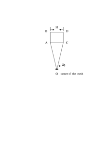
FIG. 1.: Diagram illustration of the thermal neutron interference route. We assume the arms AB, BD, AC and CD to be same, i.e., AB = BD = AC = CD = H. OA and OC represent the radius of the earth and the angle between OA and OC is $\delta\phi$.

REFERENCES

- [1] K. Zuber, Phys. Rep. 305, 295 (1998).
- [2] S. Bilenky, C. Giunti and W. Grimus, Phenomenology of neutrino oscillation (hep-ph/9812360).
-
[3]
Y. Fukuda et al., Phys. Rev. Lett. 81, 1158 (1998);
Y. Fukuda et al., Phys. Rev. Lett. 81, 1562 (1998);
Y. Fukuda et al., Phys. Rev. Lett. 82, 1810 (1999). - [4] J. Wudka, Mod. Phys. Lett. A6, 3291 (1991).
- [5] D. V. Ahluwalia and C. Burgard, Gen. Rel. and Grav., 28, 1161 (1996).
- [6] L. Wolfenstein, Phys. Rev. D 17, 2369 (1978); S. Mikheyev and A. Yu. Smirnov, Nuovo Cimento Soc. Ital. Fis. C 9, 17 (1986).
- [7] M.Gasperini, Phys. Rev. D39, 3606 (1989); A. Halprin and C.N. Leung, Phys. Rev. Lett.67, 1833 (1991).
- [8] J.R. Mureika and R.B. Mann, Phys. Rev. D. 54, 2761 (1996).
- [9] D. Píriz, M. Roy, and J. Wudka, Phys. Rev. D 54, 1587 (1996).
- [10] Y. Grossman and H. J. Lipkin, Phys. Rev. D. 55, 2760 (1997).
- [11] C.Y. Cardall and G.M. Fuller, Phys. Rev. D 55, 7960 (1996).
- [12] T. Bhattacharya, S. Habib, and E. Mottola, Phys. Rev. D59, 067301 (1999).
- [13] N. Fornengo, C. Giunti, C. W. Kim, and J.Song, Phys. Rev. D 56, 1895 (1997).
- [14] C. Giunti, C.W. Kim and U.W. Lee, Phys. Rev. D44, 3636 (1991); C.W. Kim and A. Pevsner, ”Neutrinos in Physics and Astrophysics”, Contemporary Concepts in Physics, vol. 8 ed. by H. Feshbach (Harwood Academic Chur), Switzerland, 1993; C. Giunti, C.W. Kim, Phys. Rev. D58, 017301 (1998).
- [15] J. Audretsch, J. Phys. A, 14, 411 (1981).
-
[16]
P.A.M. Dirac, Proc. Roy. Soc. London, 117A, 610
(1928); 118A, 351(1928); V. Fock, and D. Ivenenko, Compt.
Rend.,188, 1470 (1929); V. Fock, Zeits, Phys., 57, 261
(1929).
D. R. Brill and J. A. Wheeler, Rev. Mod. Phys. 29, 465. -
[17]
J. Anandan, Phys. Rev. D 15, 1448 (1977);
J. Anandan, IL NUOVO CIMENTO 53A, 221 (1979). - [18] F. Boehm, and P. Vogel, Physics of Massive Neutrinos (Cambridge University Press, Cambridge, 1992).
- [19] J. N. Bahcall, Neutrino Astrophysics (Cambridge University Press, Cambridge, 1994).
- [20] L. Stodolsky, Gen. Rel. and Grav., 11, 391 (1979).
- [21] J. Nitsch, and Hehl, F.W., Phys. Lett. B 15, 1448 (1981).
- [22] C.W. Misner, K.S. Thorne and J.A. Wheeler, Gravitation (W.H. Freeman and Company, San Francisco, 1973); S. W. Weinberg, Gravitation and Cosmology (Wiley, New York, 1972); H.C. Ohanian, and R. Ruffini, Gravitation and Spacetime (Norton & Company, New York, 1994).
- [23] H. Lipkin, Phys. Lett. B 348, 604 (1995); H. Lipkin, “Quantum mechanics of neutrino oscillation”, hep-ph/9901399.
- [24] J. J. Sakurai, Modern Quantum Mechanics (Benjamin/Cummings, New York, 1985).
- [25] R. Colella, A.W. Overhauser, and S.A. Werner, Phys. Rev. Lett. 34, 1472 (1975); D. M. Greenberger, Rev. Mod. Phys., 55, 875 (1983); S. A. Werner, H. Kaiser, M. Arif and R. Clothier, Physica B, 151, 22 (1988).
- [26] K. Hayashi and T. Shirafuji, Phys. Rev. D 19, 3524 (1979).