Feynman Diagrams of Generalized Matrix Models and the Associated Manifolds in Dimension 4

Abstract

The problem of constructing a quantum theory of gravity has been tackled with very different strategies, most of which relying on the interplay between ideas from physics and from advanced mathematics. On the mathematical side, a central rôle is played by combinatorial topology, often used to recover the space-time manifold from the other structures involved. An extremely attractive possibility is that of encoding all possible space-times as specific Feynman diagrams of a suitable field theory. In this work we analyze how exactly one can associate combinatorial 4-manifolds to the Feynman diagrams of certain tensor theories.

PACS: 04.60.Nc, 02.40.Sf
MSC (2000): 57Q05 (primary), 57M99 (secondary).

1 Introduction

We describe in this paper precise conditions which allow to associate a four-dimensional manifold to a Feynman diagram of a rank-four tensor theory. The question originates from the attempt of formulating a quantum theory of gravity [1] in terms of a generalization of the matrix model formulation of two-dimensional quantum gravity [2]. We try to keep our discussion as much as possible independent of dimension, but we only give precise conditions in dimension two, three and four. The result was actually previously known in dimension two and three, but the fact that we can give a unified treatment allows us to clarify better the specific conditions which we exhibit in dimension four.

To give an $n$-dimensional theory of Euclidean quantum gravity one needs to define a path integral of the following form over equivalence classes of metrics:

$$Z[\Lambda,G]=\sum_{M\in{\rm Top}_{n}}\ \ \int\limits_{{\rm Riem}(M)/{\rm Diff}(M)}\mathcal{D}[g]\;{\rm e}^{-S_{g}[\Lambda,G]}\;.$$ (1)

Here ${\rm Riem}(M)/{\rm Diff}(M)$ is the space of Riemannian metrics over $M$ modulo diffeomorphism, the weight factor $S_{g}[\Lambda,G]$ is the standard Einstein-Hilbert action

$$S_{g}[\Lambda,G]=\int_{M}\!\!\sqrt{g}d^{n}\!x\left(-\frac{1}{16\pi G}R[g]+\Lambda\right)\;,$$

and a sum over all possible $n$-dimensional topologies has also been included. Formal expressions like (1) have demonstrated extremely powerful heuristic tools in theoretical physics but, as a matter of fact, they generally lack a proper definition. To actually give a definition one typically needs to be more specific and restrictive about the class ${\rm Top}_{n}$ of manifolds under consideration, and about the space ${\rm Riem}(M)/{\rm Diff}(M)$ of metrics. A possible strategy is to consider triangulated manifolds and to approximate path integration over inequivalent Riemannian structures with summation over inequivalent triangulations of the manifold. Here a triangulation ${\cal T}$ is considered to define the singular Riemannian structure in which all $n$-simplices are flat and have edges of a given length $a$. The action takes the form

$$S(\Lambda,G;{\cal T}) = k_{n}\nu_{n}({\cal T})-h_{n-2}\nu_{n-2}({\cal T})$$ (2)

where $\nu_{i}({\cal T})$ is the number of $i$-simplices in ${\cal T}$ and $k_{i}$, $h_{i}$ are given as follows in terms of the volume $\mathrm{vol}(\sigma^{i})$ of the flat $i$-simplex with edges having length $a$:

$$\begin{array}[]{lcl}k_{n}&=&\Lambda\cdot\mathrm{vol}(\sigma^{n})+\frac{n(n+1)}{2}\frac{\arccos(1/n)}{16\pi G}\mathrm{vol}(\sigma^{n-2}),\\ h_{n-2}&=&\frac{1}{8G}\mathrm{vol}(\sigma^{n-2}).\end{array}$$

This approach is known as ‘Dynamical Triangulation’ (see [3] for discussion and references) and the partition function $Z[\Lambda,G]$ is given by

$$Z_{{\rm DT}}[\Lambda,G]=\sum_{M\in{\rm Top}_{n}}\ \sum_{{\cal T}\in{\rm Tria}(M)}\;{\rm e}^{-k_{n}\nu_{n}({\cal T})+h_{n-2}\nu_{n-2}({\cal T})}.$$ (3)

Here ${\rm Tria}(M)$ denotes the set of triangulations, up to combinatorial equivalence, of a manifold $M$, and the partition function is perfectly analogous to that of (1). Note that the sum over triangulations together with the sum over topologies corresponds to the sum over all $n$-dimensional simplicial complexes which are manifolds. (As usual we consider also “singular” triangulations, i.e. we allow self-adjacencies and multiple adjacencies.) Note also that if in (1) one wants to consider the action on ${\rm Riem}(M)$ of only those diffeomorphisms which are isotopic to the identity, then the discretized analogue again has the form of (3), except that each triangulation ${\cal T}$ should now be weighted according to the number of non-isotopic ways it can be realized in the corresponding manifold.

Dynamical Triangulations have been intensively investigated in two, three and four dimensions. It is of particular interest that in two dimensions the theory may be reformulated in terms of a matrix model [2]. In the perturbative approach to this theory, the resulting Feynman diagrams have vertices which correspond to two-simplices, and propagators which correspond to edge-pairings, so a diagram leads to a surface obtained by glueing triangles. In extending the triangulation strategy to arbitrary dimension one is brought to the search for theories having Feynman diagrams in which vertices can be identified with $n$-simplices, and propagators with glueings of codimension-1 faces. If this happens then each Feynman diagram gives an $n$-dimensional simplicial complex.

Generalized matrix models with Feynman diagrams corresponding to simplicial complexes were discussed by Sasakura [4], Gross [5], Boulatov [6], Ooguri [7], and more recently by De Pietri-Freidel-Krasnov-Rovelli[8] and others. However, in all these works a complete discussion of the topological properties of the resulting simplicial complexes is missing, and the results of the present paper allow to fill this gap. More precisely, it is the aim of the present paper to introduce a specific $n$-tensor model whose Feynman diagrams can be identified with $n$-dimensional simplicial complexes, and to explicitly analyze the topological properties of these spaces. After a brief discussion of the two- and three-dimensional cases we address the four-dimensional problem. As a main result we provide an explicit criterion to decide whether the simplicial complex associated to a given Feynman diagram is a manifold or not. When the criterion is fulfilled the value of a Feynman diagram corresponds to the value of the discretized Einstein-Hilbert action of (2) on the associated triangulation. In connection with the papers mentioned above, it is worth remarking here that the weight factor of model [6] corresponds to the three dimensional Ponzano-Regge [9] model and the one of model [8] to the Barrett-Crane [10] four dimensional relativistic spin model, while in our model each Feynman graph is weighted by the simplicial action (2). Moreover, as consequence of Remark 3.2, all these models can be seen as Spin Foam [11] models.

2 Generalized matrix models and fat graphs

We review in this section the matrix model whose Feynman diagrams lead to surfaces, then we introduce more complicated models which eventually will give higher-dimensional simplicial complexes. We set up a useful graphical encoding of the Feynman diagrams, which will help us in describing how exactly a diagram leads to a simplicial complex.

Two-dimensional quantum gravity as a matrix model

The partition function of the matrix model corresponding to two-dimensional quantum gravity is

$$Z[N,\lambda]=\int[d\phi]\;{\rm e}^{-\frac{1}{2}\mathrm{Tr}[\phi^{2}]+\frac{\lambda}{3}\mathrm{Tr}[\phi^{3}]},\qquad[d\phi]=\frac{1}{\mathcal{N}}\prod_{\alpha\leq\beta}d\Re{\phi_{\alpha\beta}}\prod_{\alpha<\beta}d\Im{\phi_{\alpha\beta}}$$ (4)

where the configuration variable is a Hermitian $N\times N$ matrix $\phi=(\phi_{\alpha\beta})$, and $\mathcal{N}$ is a normalization constant chosen such that $Z[N,0]=1$. We note that the integral defining $Z[N,\lambda]$ is divergent for real $\lambda$. This means that some procedure must be given to properly define (4). For the purpose of this work we will consider $Z[N,\lambda]$ as a formal power series in $\lambda$ and we will view (4) as a formal definition of the coefficients $Z^{(\!k\!)}[N]$ such that $Z[N,\lambda]=\sum_{k}Z^{(\!k\!)}[N]\lambda^{k}/k!$, where $Z^{(\!k\!)}[N]$ corresponds to $d^{k}Z[N,\lambda]/d\lambda^{k}|_{\lambda=0}$, and is computed by interchanging integration and derivation. In the standard field-theoretical language we say that we evaluate the integral of (4) as the Feynman graph expansion (formal power series in $\lambda$) generated by

$$Z[N,\lambda]=\left.\exp\left[\frac{\lambda}{3}V^{\alpha_{1}\alpha_{2};\beta_{1}\beta_{2};\gamma_{1}\gamma_{2}}\frac{\delta}{\delta J^{\alpha_{1}\alpha_{2}}}\frac{\delta}{\delta J^{\beta_{1}\beta_{2}}}\frac{\delta}{\delta J^{\gamma_{1}\gamma_{2}}}\right]Z^{\scriptscriptstyle(0)}[N;J]\right|_{J=0}$$

$$Z^{\scriptscriptstyle(0)}[N;J]=\int[d\phi]\;{\rm e}^{-\frac{1}{2}\mathrm{Tr}[\phi^{2}]+\phi_{\alpha\beta}J^{\alpha\beta}}={\rm const}\cdot\exp\left[\frac{1}{2}J^{\alpha\beta}G_{\alpha\beta;\gamma\delta}J^{\gamma\delta}\right],\qquad$$

where the Einstein convention of sum over repeated covariant-contravariant indices is assumed, $G_{\alpha_{1}\alpha_{2};\beta_{1}\beta_{2}}=g_{\alpha_{1}\beta_{2}}\cdot g_{\alpha_{2}\beta_{1}}$, $V^{\alpha_{1}\alpha_{2};\beta_{1}\beta_{2};\gamma_{1}\gamma_{2}}=g^{\alpha_{2}\beta_{1}}\cdot g^{\beta_{2}\gamma_{1}}g^{\gamma_{2}\alpha_{1}}$, $g_{\alpha\beta}=g^{\alpha\beta}=\delta^{\alpha}_{\beta}$, where $\delta$ is the Kronecker symbol. The function $Z^{\scriptscriptstyle(0)}[N;J]$ thus defined is the free partition function in presence of the source $J$.

It is now convenient to use a graphical representation of tensor expressions containing sums over dummy indices. We will represent the metric and $\delta$ as:

$$g_{\alpha_{1}\alpha_{2}}=\begin{array}[]{c}\begin{picture}(20.0,30.0)\put(0.0,20.0){\makebox(10.0,10.0)[]{$\scriptstyle\alpha_{1}$}} \put(10.0,20.0){\makebox(10.0,10.0)[]{$\scriptstyle\alpha_{2}$}} \put(10.0,20.0){\oval(10.0,20.0)[b]} \end{picture}\end{array},\qquad g^{\beta_{1}\beta_{2}}=\begin{array}[]{c}\begin{picture}(20.0,30.0)\put(0.0,0.0){\makebox(10.0,10.0)[]{$\scriptstyle\beta_{1}$}} \put(10.0,0.0){\makebox(10.0,10.0)[]{$\scriptstyle\beta_{2}$}} \put(10.0,10.0){\oval(10.0,20.0)[t]} \end{picture}\end{array},\qquad\delta^{\alpha}_{\beta}=\begin{array}[]{c}\begin{picture}(10.0,30.0)\put(0.0,0.0){\makebox(10.0,10.0)[]{$\scriptstyle\beta$}} \put(0.0,20.0){\makebox(10.0,10.0)[]{$\scriptstyle\alpha$}} \put(5.0,10.0){\line(0,1){10.0}} \end{picture}\end{array}$$ (5)

Moreover, we will use the following symbols

$$T^{\alpha_{1}\ldots\alpha_{i}}_{\beta_{1}\ldots\beta_{j}}=\begin{array}[]{c}\begin{picture}(50.0,50.0)\put(0.0,37.0){\makebox(10.0,10.0)[]{$\scriptstyle\alpha_{1}$}} \put(20.0,37.0){\makebox(10.0,10.0)[]{$\ldots$}} \put(40.0,37.0){\makebox(10.0,10.0)[]{$\scriptstyle\alpha_{i}$}} \put(5.0,35.0){\line(0,-1){5.0}} \put(45.0,35.0){\line(0,-1){5.0}} \put(0.0,20.0){\framebox(50.0,10.0)[]{$T$}} \put(10.0,20.0){\line(0,-1){5.0}} \put(40.0,20.0){\line(0,-1){5.0}} \put(5.0,3.0){\makebox(10.0,10.0)[]{$\scriptstyle\beta_{1}$}} \put(20.0,3.0){\makebox(10.0,10.0)[]{$\ldots$}} \put(35.0,3.0){\makebox(10.0,10.0)[]{$\scriptstyle\beta_{j}$}} \end{picture}\end{array}\qquad,\qquad\prod_{i=1}^{n}\delta^{\alpha_{i}}_{\beta_{\sigma(i)}}=\begin{array}[]{c}\begin{picture}(50.0,50.0)\put(0.0,37.0){\makebox(10.0,10.0)[]{$\scriptstyle\alpha_{1}$}} \put(10.0,37.0){\makebox(10.0,10.0)[]{$\scriptstyle\alpha_{2}$}} \put(25.0,37.0){\makebox(10.0,10.0)[]{$\ldots$}} \put(40.0,37.0){\makebox(10.0,10.0)[]{$\scriptstyle\alpha_{n}$}} \put(5.0,35.0){\line(0,-1){5.0}} \put(15.0,35.0){\line(0,-1){5.0}} \put(45.0,35.0){\line(0,-1){5.0}} \put(0.0,20.0){\framebox(50.0,10.0)[]{$\sigma\;{\scriptstyle\uparrow}$}} \put(5.0,20.0){\line(0,-1){5.0}} \put(15.0,20.0){\line(0,-1){5.0}} \put(45.0,20.0){\line(0,-1){5.0}} \put(0.0,3.0){\makebox(10.0,10.0)[]{$\scriptstyle\beta_{1}$}} \put(10.0,3.0){\makebox(10.0,10.0)[]{$\scriptstyle\beta_{2}$}} \put(25.0,3.0){\makebox(10.0,10.0)[]{$\ldots$}} \put(40.0,3.0){\makebox(10.0,10.0)[]{$\scriptstyle\beta_{n}$}} \end{picture}\end{array}$$ (6)

to represent a generic tensor with $i$ contravariant and $j$ covariant indices, and a permutation $\sigma\in{\hbox{\Got S}}_{n}$, respectively. When two strands are connected by a line we assume that the strands carry the same dummy index and that summation over this index is taken. Using these conventions, the propagator and the vertex are represented by the diagrams:

$$V^{\alpha_{1}\alpha_{2};\beta_{1}\beta_{2};\gamma_{1}\gamma_{2}} \Rightarrow \begin{array}[]{c}\begin{picture}(100.0,25.0)\put(45.0,15.0){\oval(90.0,30.0)[b]} \put(25.0,15.0){\oval(30.0,24.0)[b]} \put(65.0,15.0){\oval(30.0,24.0)[b]} \put(0.0,17.0){${\scriptstyle\alpha_{1}\alpha_{2}}$} \put(40.0,17.0){${\scriptstyle\beta_{1}\beta_{2}}$} \put(80.0,17.0){${\scriptstyle\gamma_{1}\gamma_{2}}$} \end{picture}\end{array}$$

$$G_{\alpha_{1}\alpha_{2};\beta_{1}\beta_{2}} \Rightarrow \begin{array}[]{c}\begin{picture}(80.0,25.0)\put(35.0,10.0){\oval(70.0,26.0)[t]} \put(35.0,10.0){\oval(50.0,20.0)[t]} \put(0.0,0.0){${\scriptstyle\alpha_{1}\alpha_{2}}$} \put(60.0,0.0){${\scriptstyle\beta_{1}\beta_{2}}$} \end{picture}\end{array}$$

A direct inspection shows that, up to order $\lambda^{2}$, the formal power series $Z[N,\lambda]$ is given by

$$Z[N,\lambda] = 1+\lambda^{2}\left(\frac{1}{6}[[D1]]+\frac{1}{2}[[D2]]+\frac{1}{6}[[D3]]\right)+\ldots$$

$$= 1+\lambda^{2}\left(\frac{1}{6}N^{3}+\frac{1}{2}N^{3}+\frac{1}{6}N\right)+\ldots\ .$$

where $[[D1]]$, $[[D2]]$ and $[[D3]]$ are the evaluations of the Feynman diagrams of Fig. 1, carried out using the correspondence just discussed between diagrams and tensor expressions. Note that, if we associate a triangle to each vertex and an edge-glueing to each propagator as described in Fig. 1, then the two diagrams corresponding to the sphere evaluate to $N^{3}$, while the one corresponding to the torus evaluates to $N$.

Figure 1: The three inequivalent Feynman diagrams of the two-dimensional matrix model (4) at order $\lambda^{2}$. The association of triangles to vertices is explicitly shown. Interpreting each propagator as a gluing instruction between two edges of triangles, it is easy to see that $D1$ and $D2$ correspond to different triangulation of the sphere, while $D3$ corresponds to a triangulation of the torus.

Higher-rank generalized matrix models

It is possible to consider higher-dimensional extensions of the matrix model (4), using higher-rank tensors. The natural generalization of the matrix model partition function is achieved by considering as configuration variable an $n$-tensor ${\phi_{\alpha_{1}\ldots\alpha_{n}}}$, where each $\alpha_{i}$ varies between $1$ and $N$, having the following symmetry:

$$\phi_{\alpha_{\tau(1)}\ldots\alpha_{\tau(n)}}=\Re[{\phi_{\alpha_{1}\ldots\alpha_{n}}}]+i\cdot{\rm sgn}(\tau)\cdot\Im[{\phi_{\alpha_{1}\ldots\alpha_{n}}}]$$ (9)

where $\tau\in{\hbox{\Got S}}_{n}$ and ${\rm sgn}(\tau)$ is the signature (also called parity) of $\tau$. Using multi-indices ${\mathbf{\alpha}}=(\alpha_{1}\ldots\alpha_{n})$ we consider the following partition function for the $n$-tensor model

$$Z_{n}[N,\lambda]=\int[d\phi]\;\exp\left[{-\frac{1}{2}\sum_{\mathbf{\alpha}}|\phi_{\mathbf{\alpha}}|^{2}+\frac{\lambda}{n+1}\sum_{{\mathbf{\alpha}}^{\scriptscriptstyle(\!0\!)}\ldots{\mathbf{\alpha}}^{\scriptscriptstyle(\!n\!)}}V^{{\mathbf{\alpha}}^{\scriptscriptstyle(\!0\!)}\ldots{\mathbf{\alpha}}^{\scriptscriptstyle(\!n\!)}}\cdot\phi_{{\mathbf{\alpha}}^{\scriptscriptstyle(\!0\!)}}\cdot\ldots\cdot\phi_{{\mathbf{\alpha}}^{\scriptscriptstyle(\!n\!)}}}\right]$$ (10)

where $V^{{\mathbf{\alpha}}^{\scriptscriptstyle(\!0\!)}\ldots{\mathbf{\alpha}}^{\scriptscriptstyle(\!n\!)}}$ is the vertex function which will be defined in (25) below (we do not define it here because its form is not needed and because the general definition will involve notations introduced later. A definition for the three-tensor and four-tensor model will be given before the general one in (2) and (2), respectively).

As in the 2-dimensional case, the expansion of $Z_{n}[N,\lambda]$ is obtained by introducing another function $Z_{n}^{\scriptscriptstyle(0)}[N;J]$ such that

$$Z_{n}[N,\lambda]=\left.\exp\left[\frac{\lambda}{n+1}V^{{\mathbf{\alpha}}^{\scriptscriptstyle(\!0\!)}\ldots{\mathbf{\alpha}}^{\scriptscriptstyle(\!n\!)}}\frac{\delta}{\delta J^{{\mathbf{\alpha}}^{\scriptscriptstyle(\!0\!)}}}\cdots\frac{\delta}{\delta J^{{\mathbf{\alpha}}^{\scriptscriptstyle(\!n\!)}}}\right]Z_{n}^{\scriptscriptstyle(0)}[N;J]\right|_{J=0}.$$ (11)

Proposition 2.1

The free partition function in presence of source of the generalized matrix models (10) whose fundamental field fulfills the symmetry requirements (9), defined as

$$Z_{n}^{\scriptscriptstyle(0)}[N;J]=\int[d\phi]\exp\Bigg{[}-\frac{1}{2}\sum_{\alpha_{1},\ldots,\alpha_{n}}|\phi_{\alpha_{1}\ldots\alpha_{n}}|^{2}+\sum_{\alpha_{1},\ldots,\alpha_{n}}\phi_{\alpha_{1}\ldots\alpha_{n}}J^{\alpha_{1}\ldots\alpha_{n}}\Bigg{]}$$

is given by

$$Z_{n}^{\scriptscriptstyle(0)}[N;J]=\exp\left[\frac{1}{2}J^{\alpha_{1}\ldots\alpha_{n}}G_{\alpha_{1}\ldots\alpha_{n};\beta_{1}\ldots\beta_{n}}J^{\beta_{1}\ldots\beta_{n}}\right],$$ (12)

where the propagator is defined as

$$G_{\alpha_{1}\ldots\alpha_{n};\beta_{1}\ldots\beta_{n}}=\frac{2}{n!}\sum_{\begin{array}[]{c}\scriptstyle\tau\in{\hbox{\Got S}}_{n}\\[-2.84526pt] \scriptstyle{\rm sgn}(\tau)=-1\end{array}}G_{\alpha_{1}\ldots\alpha_{n};\beta_{1}\ldots\beta_{n}}^{\scriptscriptstyle(\!\tau\!)},$$ (13)

and $G_{\alpha_{1}\ldots\alpha_{n};\beta_{1}\ldots\beta_{n}}^{\scriptscriptstyle(\!\tau\!)}=\delta_{\alpha_{\tau(1)}\beta_{1}}\ldots\delta_{\alpha_{\tau(n)}\beta_{n}}$. Moreover, if integration is restricted to real $\phi$, the partition function has the same form (12) but the propagator is given by

$$G_{\alpha_{1}\ldots\alpha_{n};\beta_{1}\ldots\beta_{n}}=\frac{1}{n!}\sum_{\tau\in{\hbox{\Got S}}_{n}}G_{\alpha_{1}\ldots\alpha_{n};\beta_{1}\ldots\beta_{n}}^{\scriptscriptstyle(\!\tau\!)}$$ (14)

Proof of  2.1. The measure $[d\phi]$, as usual, is the product of the Lebesgue measures over all the independent components of $\phi$ multiplied by a normalization constant $\mathcal{N}$ such that $Z_{n}^{\scriptscriptstyle(0)}[N;0]=1$.

The symmetry requirement (9) implies that the free partition function in presence of source can be written as follows just in terms of the completely symmetrized $J^{\beta_{1}\ldots\beta_{n}}_{S}$ and the completely anti-symmetrized $J^{\beta_{1}\ldots\beta_{n}}_{A}$ parts of the source $J^{\beta_{1}\ldots\beta_{n}}$:

$$Z_{n}^{\scriptscriptstyle(0)}[N;J]$$

$$=\ \ \frac{1}{\mathcal{N}}\int\!\!\prod_{\alpha_{1}\leq\ldots\leq\alpha_{n}}\!\!d\Re{\phi_{\alpha_{1}\ldots\alpha_{n}}}\exp\Bigg{[}-\frac{1}{2}\!\sum_{\alpha_{1},\ldots,\alpha_{n}}|\Re\phi_{\alpha_{1}\ldots\alpha_{n}}|^{2}+\!\sum_{\alpha_{1},\ldots,\alpha_{n}}\Re\phi_{\alpha_{1}\ldots\alpha_{n}}J_{S}^{\alpha_{1}\ldots\alpha_{n}}\Bigg{]}\times$$

$$\ \ \ \ \qquad\times\prod_{\alpha_{1}<\ldots<\alpha_{n}}\!\!d\Im{\phi_{\alpha_{1}\ldots\alpha_{n}}}\exp\Bigg{[}-\frac{1}{2}\!\sum_{\alpha_{1},\ldots,\alpha_{n}}|\Im\phi_{\alpha_{1}\ldots\alpha_{n}}|^{2}+i\!\sum_{\alpha_{1},\ldots,\alpha_{n}}\Im\phi_{\alpha_{1}\ldots\alpha_{n}}J_{A}^{\alpha_{1}\ldots\alpha_{n}}\Bigg{]}.$$

Gaussian integration with respect to the variables $\Re\phi_{\alpha_{1}\ldots\alpha_{n}}$ and $\Im\phi_{\alpha_{1}\ldots\alpha_{n}}$ can be easily performed. The result is indeed:

$$Z_{n}^{\scriptscriptstyle(0)}[N;J]=\frac{k}{\mathcal{N}}\exp\Bigg{[}\frac{1}{2}\sum_{\alpha_{1},\ldots,\alpha_{n}}(J_{S}^{\alpha_{1}\ldots\alpha_{n}})^{2}-\frac{1}{2}\sum_{\alpha_{1},\ldots,\alpha_{n}}(J_{A}^{\alpha_{1}\ldots\alpha_{n}})^{2}\Bigg{]}$$

where $k=k(n,N)$ is a constant which takes into account the number Gaussian integrations which have been performed. It is now easy to check that, fixing $\mathcal{N}=k$, the first part of the proposition holds. Now, if the variable $\phi$ is restricted to be real, i.e. integration with respect to the $\Re\phi_{\alpha_{1}\ldots\alpha_{n}}$’s is only considered, then the term depending on $J_{A}^{\alpha_{1}\ldots\alpha_{n}}$ does not appear and this proves second part of the proposition. (Note that restricting to real $\phi$ one has to make a different choice of $\mathcal{N}$.)  2.1

Using Proposition 2.1, we can now rewrite the partition function of the $n$-tensor model in terms of its Feynman diagram expansion. In fact, combining (11) and (12), it is possible to express $Z_{n}[N,\lambda]$ as the formal power series

$$\begin{split}Z_{n}[N,\lambda]=\sum_{k}&\frac{1}{k!}\frac{\lambda^{k}}{(n+1)^{k}}V^{{\mathbf{\alpha}}^{\scriptscriptstyle(\!0\!)}\ldots{\mathbf{\alpha}}^{\scriptscriptstyle(\!n\!)}}\cdot\ldots\cdot V^{{\mathbf{\alpha}}^{\scriptscriptstyle(\!kn+k-n-1\!)}\ldots{\mathbf{\alpha}}^{\scriptscriptstyle(\!kn+k-1\!)}}\times\\ &\!\!\!\!\times\frac{(1/2)^{k(n+1)/2}}{(k(n+1)/2)!}\sum_{\sigma\in{\hbox{\Got S}}_{\{0,\ldots,kn+k-1\}}}\!\!\!\!G_{{\mathbf{\alpha}}^{\scriptscriptstyle(\!\sigma(0)\!)}{\mathbf{\alpha}}^{\scriptscriptstyle(\!\sigma(1)\!)}}\cdot\ldots\cdot G_{{\mathbf{\alpha}}^{\scriptscriptstyle(\!\sigma(kn+k-2)\!)}{\mathbf{\alpha}}^{\scriptscriptstyle(\!\sigma(kn+k-1)\!)}}\end{split}$$ (15)

where the sum over $k$ is restricted to all positive $k$’s such that $k(n+1)$ is even. The explicit form of the propagator $G_{{\mathbf{\alpha}}^{\scriptscriptstyle(\!1\!)}{\mathbf{\alpha}}^{\scriptscriptstyle(\!2\!)}}$ is given by (13), whereas the vertex has not been defined yet. Note that restricting to real $\phi$ we would have obtained the same expression with the propagator of (14).

The three-tensor and four-tensor generalized matrix model

Since our main interest is to analyze models related to quantum gravity in three and four dimensions, we provide now the explicit definition of the partition function in these two cases:

$$Z_{3}[N,\lambda] = \int[d\phi]\exp\Bigg{[}-\frac{1}{2}\sum_{\alpha_{1},\alpha_{2},\alpha_{3}}|\phi_{\alpha_{1}\alpha_{2}\alpha_{3}}|^{2}$$

$$\qquad\qquad+\frac{\lambda}{4}\sum_{\alpha_{1},\ldots,\alpha_{6}}\phi_{\alpha_{1}\alpha_{2}\alpha_{3}}\phi_{\alpha_{4}\alpha_{5}\alpha_{3}}\phi_{\alpha_{4}\alpha_{2}\alpha_{6}}\phi_{\alpha_{1}\alpha_{5}\alpha_{6}}\Bigg{]}$$

$$Z_{4}[N,\lambda] = \int[d\phi]\exp\Bigg{[}-\frac{1}{2}\sum_{\alpha_{1},\ldots,\alpha_{4}}|\phi_{\alpha_{1}\alpha_{2}\alpha_{3}\alpha_{4}}|^{2}$$

$$\qquad\qquad+\frac{\lambda}{5}\sum_{\alpha_{1},\ldots,\alpha_{10}}\phi_{\alpha_{1}\alpha_{2}\alpha_{3}\alpha_{4}}\phi_{\alpha_{4}\alpha_{5}\alpha_{6}\alpha_{7}}\phi_{\alpha_{7}\alpha_{3}\alpha_{8}\alpha_{9}}\phi_{\alpha_{9}\alpha_{6}\alpha_{2}\alpha_{10}}\phi_{\alpha_{10}\alpha_{8}\alpha_{5}\alpha_{1}}\Bigg{]}$$

Using the graphic presentation defined by (5) and (6), the Feynman rules of the two models (2) and (2) are illustrated respectively in Fig. 2 and in Fig. 3.

Figure 2: Feynman rules of the 3-tensor generalized matrix model. The analogy of the vertex diagram with the tetrahedron is explicitly shown.

Remark 2.2

The choice of indices in the last term of (2) may appear to be a weird one, since it leads to the vertex picture of Fig. 2, in which two of the ends of the vertex have a seemingly unnatural torsion. An explanation of this choice will be given in Remark 3.1.

Figure 3: Feynman rules of the 4-tensor generalized matrix model. The analogy of the vertex diagram with the 4-simplex is explicitly shown.

Encoding of Feynman diagrams: fat graphs

We introduce in this paragraph labeled graphs which conveniently encode the Feynman diagrams arising from the models discussed above.

Definition 2.3

A fat $n$-graph is a connected $(n+1)$-valent graph with the following additional structures: all the edges are oriented and labeled by a permutation in ${\hbox{\Got S}}_{n}$, and at each vertex the $n+1$ initial portions of edge emanating from the vertex are numbered by $0,1,\dots,n$. We will denote by $\textsf{FG}_{n}$ the set of all fat $n$-graphs up to homeomorphisms which preserve all structures.

A practical way of describing a fat $n$-graph, which we will always use, is as follow. We take an immersion (possibly with double points) of the graph in ${\hbox{\Bbb R}}^{2}$, in such a way that at each vertex all the edges start with a positive upward component of the velocity, as in (22) below. Then the numbering $0,1,\dots,n$ is simply taken from left to right. Direction and label of an edge are marked on the edge itself.

Definition 2.4

A fat $n$-graph is said to be oriented if all its edges are labeled by even permutations. The set of all such graphs is denoted by $\textsf{FG}_{n}^{+}$.

It is now straight-forward to encode the Feynman diagram expansion (15) of the $n$-tensor model in terms of a sum over all fat $n$-graphs. We proceed as follows. We first label all the initial portions of edges by a multi-index $k$. We then associate tensor expressions to vertices and edges of the fat graph, according to the following rules:

$$\begin{array}[]{c}\begin{picture}(70.0,35.0)\put(0.0,0.0){\makebox(10.0,10.0)[]{${\scriptscriptstyle(\!j\!)}$}} \put(20.0,10.0){\oval(30.0,30.0)[tl]} \put(20.0,25.0){\vector(1,0){30.0}} \put(30.0,27.0){\makebox(10.0,10.0)[]{$\sigma$}} \put(50.0,10.0){\oval(30.0,30.0)[tr]} \put(60.0,0.0){\makebox(10.0,10.0)[]{${\scriptscriptstyle(\!i\!)}$}} \end{picture}\end{array}\Rightarrow G^{\scriptscriptstyle(\!\tau\!)}_{{\mathbf{\alpha}}^{\scriptscriptstyle(\!j\!)}{\mathbf{\alpha}}^{\scriptscriptstyle(\!i\!)}}\qquad,\qquad\begin{array}[]{c}\begin{picture}(80.0,35.0)\put(40.0,15.0){\oval(70.0,30.0)[b]} \put(40.0,15.0){\oval(40.0,30.0)[b]} \put(40.0,0.0){\circle*{3.0}} \put(35.0,10.0){\makebox(10.0,10.0)[]{$\ldots$}} \put(5.0,7.0){\makebox(10.0,10.0)[]{$\scriptstyle 0$}} \put(20.0,7.0){\makebox(10.0,10.0)[]{$\scriptstyle 1$}} \put(75.0,7.0){\makebox(10.0,10.0)[]{$\scriptstyle n$}} \put(0.0,20.0){\makebox(10.0,10.0)[]{${\scriptscriptstyle(\!i_{0}\!)}$}} \put(15.0,20.0){\makebox(10.0,10.0)[]{${\scriptscriptstyle(\!i_{1}\!)}$}} \put(70.0,20.0){\makebox(10.0,10.0)[]{${\scriptscriptstyle(\!i_{n}\!)}$}} \end{picture}\end{array}\Rightarrow V^{{\mathbf{\alpha}}^{\scriptscriptstyle(\!i_{0}\!)}\ldots{\mathbf{\alpha}}^{\scriptscriptstyle(\!i_{n}\!)}}$$ (20)

where $\tau=\sigma\circ(1\;n)$. In this way we obtain a tensor expression in which each multi-index ${\mathbf{\alpha}}^{\scriptscriptstyle(\!i\!)}$ appears exactly twice. We denoted by $[[G]]$ the sum over all the possible values of the multi-indices ${\mathbf{\alpha}}^{\scriptscriptstyle(\!i\!)}$ of this tensor expression.

Using the definition just given, we can now plug into (15) the explicit formula for the propagators given in Proposition 2.1, and rewrite $Z_{n}[N,\lambda]$ as a sum over all fat $n$-graphs. One only needs to be careful about multiplicities. Denoting by $\nu_{0}(G)$ and $\nu_{1}(G)$ the numbers of vertices and edges of a fat graph $G$, the right expression is computed to be

$$Z_{n}[N,\lambda] = 1+\sum_{G\in\textsf{FG}_{n}^{+}}\ w_{n}(G)\cdot\lambda^{\nu_{0}(G)}\cdot[[G]],$$ (21)

$$w_{n}(G) = \frac{\mu(G)}{\nu_{0}(G)!\cdot(n+1)^{\nu_{0}(G)}\cdot(n!)^{\nu_{1}(G)}},$$

where $\mu(G)$ is the number of the inequivalent ways of labeling the vertices of $G$ with $\nu_{0}(G)$ symbols. Note also that $\nu_{1}(G)=(n+1)\nu_{0}(G)/2$, and that the factors $\nu_{1}(G)!$ and $2^{\nu_{1}(G)}$ originally appearing in (15) get simplified during the computation.

3 Complex associated to a fat graph

Given a finite set ${\cal S}$ of (disjoint) simplices, all having the same dimension, we call face-pairing ${\cal P}$ on ${\cal S}$ a set of simplicial homeomorphisms between codimension-1 faces of the elements of ${\cal S}$, where each such face appears exactly once as the source or target of a homeomorphism. We interpret ${\cal P}$ as a set of glueing instructions between the simplices of ${\cal S}$, and we denote by ${\cal S}/{\cal P}$ the space resulting from the glueing. We will often implicitly assume that ${\cal S}/{\cal P}$ is connected. We will denote by $\textsf{GS}_{n}$ the set of all spaces of the form ${\cal S}/{\cal P}$ where all the elements of ${\cal S}$ are $n$-simplices. So an element of $\textsf{GS}_{n}$ is a simplicial complex with a fixed “singular” triangulation.

We now define a map from the set $\textsf{FG}_{n}$ of fat $n$-graphs to the set $\textsf{GS}_{n}$ of spaces obtained by glueing $n$-simplices. To each vertex $v$ of $G\in\textsf{FG}_{n}$ we associate an $n$-simplex $S(v)$ with vertices labeled $p_{i}(v)$, $i=0,\ldots,n$. To each initial portion of edge at $v$ we associate an $(n-1)$-face of $S(v)$, according to the rule

$$\begin{array}[]{c}\begin{picture}(180.0,50.0)\put(0.0,35.0){\makebox(10.0,10.0)[]{$\theta(p_{0}(v)$)}} \put(45.0,35.0){\makebox(10.0,10.0)[]{$\theta(p_{1}(v)$)}} \put(90.0,30.0){\oval(160.0,40.0)[b]} \put(90.0,30.0){\oval(80.0,40.0)[b]} \put(85.0,0.0){\makebox(10.0,10.0)[]{$v$}} \put(90.0,10.0){\circle*{4.0}} \put(90.0,30.0){\oval(30.0,40.0)[bl]} \put(100.0,20.0){\makebox(10.0,10.0)[]{$\cdots$}} \put(165.0,35.0){\makebox(10.0,10.0)[]{$\theta(p_{n}(v)$)}} \end{picture}\end{array}$$ (22)

where $\theta(p_{i}(v))$ represents the face opposite to $p_{i}(v)$. Each edge of $G$ determines a pairing (simplicial identification) between the $(n\!-\!1)$-faces associated to its ends, as described now. First, to each vertex of $G$ we associate the following object:

$$\begin{array}[]{c}\begin{picture}(250.0,50.0)\put(28.0,15.0){\makebox(0.0,0.0)[bl]{$\theta(p_{0}(v)$)}} \put(5.0,30.0){\line(1,0){40.0}} \put(5.0,35.0){\line(0,-1){5.0}} \put(0.0,37.0){\makebox(10.0,10.0)[]{$\scriptstyle i_{1}^{0}$}} \put(15.0,35.0){\line(0,-1){5.0}} \put(10.0,37.0){\makebox(10.0,10.0)[]{$\scriptstyle i_{2}^{0}$}} \put(25.0,37.0){\makebox(10.0,10.0)[]{$\ldots$}} \put(45.0,35.0){\line(0,-1){5.0}} \put(40.0,37.0){\makebox(10.0,10.0)[]{$\scriptstyle i_{n}^{0}$}} \put(98.0,15.0){\makebox(0.0,0.0)[bl]{$\theta(p_{1}(v)$)}} \put(75.0,30.0){\line(1,0){40.0}} \put(75.0,35.0){\line(0,-1){5.0}} \put(70.0,37.0){\makebox(10.0,10.0)[]{$\scriptstyle i_{1}^{1}$}} \put(85.0,35.0){\line(0,-1){5.0}} \put(80.0,37.0){\makebox(10.0,10.0)[]{$\scriptstyle i_{2}^{1}$}} \put(95.0,37.0){\makebox(10.0,10.0)[]{$\ldots$}} \put(115.0,35.0){\line(0,-1){5.0}} \put(110.0,37.0){\makebox(10.0,10.0)[]{$\scriptstyle i_{n}^{1}$}} \put(228.0,15.0){\makebox(0.0,0.0)[bl]{$\theta(p_{n}(v)$)}} \put(205.0,30.0){\line(1,0){40.0}} \put(205.0,35.0){\line(0,-1){5.0}} \put(200.0,37.0){\makebox(10.0,10.0)[]{$\scriptstyle i_{1}^{n}$}} \put(215.0,35.0){\line(0,-1){5.0}} \put(210.0,37.0){\makebox(10.0,10.0)[]{$\scriptstyle i_{2}^{n}$}} \put(225.0,37.0){\makebox(10.0,10.0)[]{$\ldots$}} \put(245.0,35.0){\line(0,-1){5.0}} \put(240.0,37.0){\makebox(10.0,10.0)[]{$\scriptstyle i_{n}^{n}$}} \put(125.0,0.0){\circle*{4.0}} \put(125.0,30.0){\oval(200.0,60.0)[b]} \put(125.0,30.0){\oval(60.0,60.0)[b]} \put(125.0,30.0){\oval(100.0,60.0)[br]} \put(160.0,20.0){$\cdots$} \end{picture}\end{array}$$ (23)

where the sequence $(i_{1}^{k},i_{2}^{k},\cdots,i_{n}^{k})$ depends on whether $n\cdot k$ is even or odd. If $n\cdot k$ is even then the sequence is $(k-1,k-2,\cdots,k-n)$, with indices meant modulo $n+1$, while if $n\cdot k$ is odd then the sequence is $(k+1,k+2,\cdots,k+n)$, with indices again modulo $n+1$. Now an edge of $G$ can be pictured as follows:

$$\begin{array}[]{c}\begin{picture}(200.0,60.0)\put(25.0,5.0){\line(0,1){10.0}} \put(27.0,0.0){$\theta(p_{j_{0}}\!(v))$} \put(5.0,15.0){\line(1,0){40.0}} \put(5.0,20.0){\line(0,-1){5.0}} \put(0.0,22.0){\makebox(10.0,10.0)[]{$\scriptstyle j_{1}$}} \put(15.0,20.0){\line(0,-1){5.0}} \put(10.0,22.0){\makebox(10.0,10.0)[]{$\scriptstyle j_{2}$}} \put(25.0,22.0){\makebox(10.0,10.0)[]{$\ldots$}} \put(45.0,20.0){\line(0,-1){5.0}} \put(40.0,22.0){\makebox(10.0,10.0)[]{$\scriptstyle j_{n}$}} \put(40.0,35.0){\oval(30.0,30.0)[tl]} \put(40.0,50.0){\vector(1,0){70.0}} \put(70.0,52.0){\makebox(10.0,10.0)[]{$\sigma$}} \put(110.0,35.0){\oval(30.0,30.0)[tr]} \put(125.0,5.0){\line(0,1){10.0}} \put(127.0,0.0){$\theta(p_{i_{0}}\!(w))$} \put(105.0,15.0){\line(1,0){40.0}} \put(105.0,20.0){\line(0,-1){5.0}} \put(100.0,22.0){\makebox(10.0,10.0)[]{$\scriptstyle i_{1}$}} \put(115.0,20.0){\line(0,-1){5.0}} \put(110.0,22.0){\makebox(10.0,10.0)[]{$\scriptstyle i_{2}$}} \put(125.0,22.0){\makebox(10.0,10.0)[]{$\ldots$}} \put(145.0,20.0){\line(0,-1){5.0}} \put(140.0,22.0){\makebox(10.0,10.0)[]{$\scriptstyle i_{n}$}} \end{picture}\end{array}$$ (24)

and we associate to the edge the map from $\theta(p_{i_{0}}(v))$ to $\theta(p_{j_{0}}(w))$ which maps $p_{i_{k}}(v)$ to $p_{j_{\tau(k)}}(w)$ where $\tau=\sigma\circ(1\;n)$. Summing up, we have associated to $G\in\textsf{FG}_{n}$ a set ${\cal S}$ of $n$-simplices and a face-pairing ${\cal P}$ on this set. The result is then a triangulated complex ${\cal S}/{\cal P}$, so indeed a map $\textsf{FG}_{n}\to\textsf{GS}_{n}$ has been defined.

Remark 3.1

If we give to $S(v)$ the orientation induced by the ordering $p_{0}(v)$, $p_{1}(v)$, …, $p_{n}(v)$, and to its faces the orientation as portions of the boundary, then the ordering chosen in (23) is always a positive one. In particular, a face-glueing as in (24) reverses the induced orientation precisely when $\sigma\in{\hbox{\Got S}}_{n}$ is an even permutation. This explains Fig. 2 and answers the naturality issue raised in Remark 2.2.

Remark 3.2

Taking Fig. 2 and Fig. 3 as models, one can rather easily turn (23) and (24) into rules which allow to associate to a fat graph $G$ a pattern of circuits (i.e. maps from the circle) on the graph. If there are $\nu_{2}(G)$ of these circuits and we attach $\nu_{2}(G)$ discs $D^{2}$ to $G$ along them, we get a polyhedron with precisely three types of points. Namely, the neighbourhood of a point is either a plane, or the union of $n$ half-planes with common boundary line, or the infinite cone over the 1-skeleton of an $n$-simplex. It is not hard to see that this polyhedron is actually the 2-skeleton of the cellularization dual to the triangulation defined by the graph as just explained. We can then interpret the fat graph as a way of describing the dual 2-skeleton of a triangulation. In particular, this dual 2-skeleton determines the triangulation itself. Note that, in general, a simplicial complex is not determined by the 2-skeleton dual to the decomposition into simplices. This is however true if the complex is obtained by glueing codimension-1 faces of simplices, as in the case of complexes defined by fat graphs.

Remark 3.3

For a triangulation of a manifold it is always automatically true that it is obtained by glueing codimension-1 faces of simplices. Moreover, if the manifold has empty boundary, any codimension-1 face belongs to precisely two simplices (or to only one but with multiplicity two). So the triangulation defines an element of $\textsf{GS}_{n}$, and in particular it comes from a fat graph.

Remark 3.4

As already mentioned, the geometric construction described in this section can be used to define a map $\textsf{FG}_{n}\to\textsf{GS}_{n}$. Any space presented as ${\cal S}/{\cal P}$ arises from some fat graph, so the map is surjective. Moreover, given an element of $\textsf{GS}_{n}$, if we choose a direction for the glueings and a numbering from $0$ to $n$ of the vertices of each simplex, a unique fat graph is determined. This shows that the map $\textsf{FG}_{n}\to\textsf{GS}_{n}$ is a bijection, provided one defines on $\textsf{FG}_{n}$ the equivalence relation which corresponds to the arbitrariness of the choices just described. In other words, up to taking the appropriate identifications, a fat graph and a space obtained by glueing simplices are one and the same thing.

Equivalence of fat graphs

We describe here how to turn the map $\textsf{FG}_{n}\to\textsf{GS}_{n}$ into a bijection. Let us first spell out the equivalence relation implicit in the definition of $\textsf{GS}_{n}$. Two spaces ${\cal S}/{\cal P}$ and ${\cal S}^{\prime}/{\cal P}^{\prime}$ are identified if they are combinatorially equivalent, namely if there exists a simplicial isomorphism $\phi:{\cal S}\to{\cal S}^{\prime}$ such that each glueing of ${\cal P}$ corresponds via $\phi$ to one of ${\cal P}^{\prime}$ or to the inverse of one of ${\cal P}^{\prime}$. The equivalence relation on $\textsf{FG}_{n}$ needed to make $\textsf{FG}_{n}\to\textsf{GS}_{n}$ bijective is now generated by two moves. The first move consists in reversing the direction of an edge and at the same time replacing its colour $\sigma$ by $(1\;n)\cdot\sigma^{-1}\cdot(1\;n)$. The second move takes place at a vertex and depends on the choice of $\lambda\in{\hbox{\Got S}}_{\{0,\dots,n\}}$, as described in Fig. 4-left,

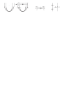
Figure 4: The move which corresponds to a change of numbering of vertices of a simplex

where as usual $\,\downarrow\!\lambda\,$ means that the $i$-th strand on the bottom is matched with the $\lambda(i)$-th strand on the top. Here $\lambda^{(i)}:\{0,\ldots,n\}\setminus\{i\}\to\{0,\ldots,n\}\setminus\{\lambda(i)\}$ is just the restriction of $\lambda$, and its action on strands is defined as above, as suggested in Fig. 4-centre. For the sake of simplicity in Fig. 4-centre we have assumed that both $n\cdot i$ and $n\cdot\lambda(i)$ are even; in general the rule described after (23) should be employed. Note that after the second move some edges can have multiple colours. To get rid of them, one should employ the (very natural) association rule described in Fig. 4-right (but note that to apply the rule one may first need to reverse the direction of the edge, using the first move).

General vertex function

We can now provide the general definition of the vertex function to be used in (10), so that it translates precisely (23) under the correspondence between fat graphs and tensor expressions defined in (5) and (6). Namely, we define

$$V^{{\mathbf{\alpha}}^{\scriptscriptstyle(\!0\!)}\ldots{\mathbf{\alpha}}^{\scriptscriptstyle(\!n\!)}}=\prod_{r<s}\delta^{\alpha^{\scriptscriptstyle(\!r\!)}_{m(r,s)}\alpha^{\scriptscriptstyle(\!s\!)}_{n(r,s)}}$$ (25)

where $m(r,s)$ and $n(r,s)$ are implicitly defined by the condition that, using the sequence $i^{k}_{l}$ defined in (23), $i^{r}_{m(r,s)}=s$ and $i^{s}_{n(r,s)}=r$, respectively. So for instance when $n$ is even we have that $m(r,s)$ and $n(r,s)$ are given respectively by $r-s$ modulo $n+1$ and $s-r$ modulo $n+1$. Of course this definition is coherent with the vertex function already defined in the case of rank-3 and rank-4 tensor models given in Fig. 2 and Fig. 3, respectively.

We go back now to (3) and (21), in order to compare them. First of all we note that, by the very choice of the vertex function of (25), the evaluation of the tensor expression corresponding to a fat $n$-graph $G$ involves the computation of precisely $\nu_{2}(G)$ traces of the Kronecker $\delta$, so $[[G]]=N^{\nu_{2}(G)}$. Here $\nu_{2}(G)$ is the number of circuits determined on the graph $G$ by equations (23) and (24) as already explained in Remark 3.2. In the same remark we have also noted that $\nu_{2}(G)$ is precisely the number of codimension-2 faces of the complex associated to $G$. Note that the evaluation is indeed invariant under the moves which define the equivalence relation on $\textsf{FG}_{n}$. This shows that when $G$ defines a manifold with a triangulation ${\cal T}$, the evaluation $[[G]]$ which appears in (21) is precisely the same as the evaluation $\exp(-k_{n}\nu_{n}({\cal T})+h_{n-2}\nu_{n-2}({\cal T}))$ of ${\cal T}$ which appears in (3), provided one chooses the constants in such a way that $h_{n-2}=\log N$ and $k_{n}=-\log(\lambda)$.

Summing up, with the choice of constants just described, we can split the sum in (21) according to whether $G\in\textsf{GS}_{n}^{+}$ defines a manifold or not (in the latter case we will just write $G\not\in{\rm Top}_{n}$ for the sake of simplicity). Namely:

$$\begin{split}Z_{n}[N,\lambda]=1&+\sum_{M\in{\rm Top}_{n}^{+}}\ \sum_{{\cal T}\in{\rm Tria}(M)}w_{n}({\cal T})\;{\rm e}^{-k_{n}\nu_{n}({\cal T})+h_{n-2}\nu_{n-2}({\cal T})}\\ &+\sum_{G\in\textsf{GS}_{n}^{+},\ G\not\in{\rm Top}_{n}}\ w_{n}(G)\cdot\lambda^{\nu_{0}(G)}\cdot N^{\nu_{2}(G)}.\end{split}$$ (26)

where the weight of ${\cal T}$ is computed by picking any $G\in\textsf{FG}_{n}^{+}$ which defines ${\cal T}$, and setting $w_{n}({\cal T})$ equal to $w_{n}(G)$ times the number of all different such $G$’s. This number is of course just equal to the number of different elements of $\textsf{FG}_{n}^{+}$ which are equivalent to $G$ under the moves defined in the previous paragraph.

Equation (26) shows that, to understand the exact relation between the partition function of the $n$-tensor model and that of the Dynamical Triangulation, one needs to be able to tell which elements of $\textsf{GS}_{n}^{+}$ define $n$-manifolds. This is the topic of next section, where we deal with the more general case of $\textsf{GS}_{n}$, which would arise anyway by restricting to a real integration variable in the partition function (10).

4 Simplicial glueings which define manifolds

The discussion of the preceding sections motivates a purely topological question, to state which we set up notations which will be used throughout this section. Fix an integer $n$ and consider a finite number of copies ${\cal S}=\{\Delta_{1},\dots,\Delta_{k}\}$ of the standard $n$-simplex. Let ${\cal P}$ be a face-pairing on ${\cal S}$, denote ${\cal S}/{\cal P}$ by $X$ and let $\pi:{\cal S}\to X$ be the natural projection. Let $X^{*}$ be the space obtained from $X$ by removing the projection of the vertices of the $\Delta_{i}$’s.

Question 4.1

When is $X$ a (closed) $n$-manifold?

Question 4.2

When is $X^{*}$ an (open) $n$-manifold?

A remark is in order. The reason why we consider also $X^{*}$ and not $X$ only is that a satisfactory answer exists for $X$ only if $n\leq 3$, while if $n=4$ we can provide such an answer for $X^{*}$ but not for $X$. Moreover the answer for $X^{*}$ and $n=3$ is very easily expressed.

PL category

Before proceeding we need to be more specific about the category in which we ask our questions. Since we are dealing with simplices, the obvious category to use is the piecewise-linear one (PL for short). All the definitions and results we will mention about PL topology may be found in [12]

The space $X$ has an obvious (finite) PL structure. Note however that the projections of the $\Delta_{i}$’s do not provide in general a triangulation of $X$, because the restriction of $\pi$ to $\Delta_{i}$ may well be non-injective. However, if we triangulate each $\Delta_{i}$ using a fine enough subdivision, we do get a triangulation in the projection. (One sees that $n$ iterations of the barycentric subdivision always suffice, but we do not insist on this point.)

The space $X^{*}$ also has a PL structure, obtained by choosing (infinite but locally finite) triangulations of the $\Delta_{i}^{*}=\Delta_{i}\setminus\{{\rm vertices}\}$, in a way which is consistent with the glueings. Rather than providing the details of this construction, we show how to realize $X^{*}$ as a subset of another polyhedron $X^{\partial}$, which will allow us to understand $X^{*}$ better. Let us consider in $\Delta_{i}$ the second barycentric subdivision, and let us remove the open stars of the original vertices, thus getting a polyhedron $\Delta_{i}^{\partial}$. (Recall that the star of a vertex in a simplicial complex is the union of all the simplices containing the vertex; for the open star only the interior of these simplices is taken.) Since the elements of ${\cal P}$ are simplicial maps, they restrict to glueings between the $\Delta_{i}^{\partial}$’s. We denote by $X^{\partial}$ space resulting from these glueings. Of course $X^{\partial}$ has a (finite) PL structure. It easily follows that $X^{*}$ embeds in $X^{\partial}$ as an open subset (see Remark 4.7 below). The natural question to ask about $X^{\partial}$ is now:

Question 4.3

When is $X^{\partial}$ a (compact) $n$-manifold (with boundary)?

Another natural question is:

Question 4.4

Provided $X$ (or $X^{\partial}$) is a manifold, when is it orientable?

The answer to this question is actually easy. Knowing that a common codimension-1 face is induced opposite orientations from two adjacent simplices, we are led to the following condition on $({\cal S},{\cal P})$ and the subsequent straight-forward result:

1. Up to reversing the natural orientation of some of the $\Delta_{i}$’s, all face-pairings in ${\cal P}$ reverse the induced orientation.

(Ori stands here for ‘Orientability of the manifold.’)

Proposition 4.5

Let $X$ and $X^{\partial}$ be manifolds. They are orientable if and only if Ori holds.

To face the other questions raised we will need to recall what a PL $n$-manifold exactly is, but we first state the result which clarifies the mutual relations. We will give a proof at the end of this section, after having acquainted the reader to the basic techniques of PL topology.

Proposition 4.6

1. $X^{*}$ is an open $n$-manifold if and only if $X^{\partial}$ is a compact $n$-manifold with boundary, and in this case $X^{*}$ is homeomorphic to $X^{\partial}\setminus\partial X^{\partial}$.

2. $X$ is a closed $n$-manifold if and only if $X^{\partial}$ is a compact $n$-manifold with boundary and all the components of $\partial X^{\partial}$ are homeomorphic to $S^{n-1}$.

Using this proposition we will only focus henceforth on $X$ and $X^{*}$, leaving $X^{\partial}$ in the background.

So, let us start with some basics of PL topology. Let $X$ be a polyhedron with a triangulation ${\cal K}$, and let $p\in X$. Assuming first $p$ is a vertex of ${\cal K}$, we define its link as

$${\rm lk}_{\cal K}(p)=\bigcup\Big{\{}\sigma\in{\cal K}:p\not\in\sigma,\ \exists\tau\in{\cal K}\ {\rm s.t.}\ \tau\supset\{p\}\cup\sigma\Big{\}}.$$

If $p$ is not a vertex we consider a subdivision of ${\cal K}$ in which $p$ is a vertex, and consider its link there. It is a fact that the link is independent of ${\cal K}$ up to PL homeomorphism, so we will just write ${\rm lk}_{X}(p)$. Some examples of links in a small 2-dimensional polyhedron are shown in Fig. 5.

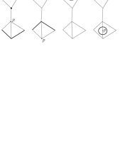
Figure 5: The links of the various points $p$ are shown in bold.

Note that the star of a point $p$, mentioned above, is just the cone from $p$ over the link of $p$. This remark motivates the following fact (which is actually often used as a definition): a polyhedron is a PL $n$-manifold if and only if the link of every point is homeomorphic either to the $(n-1)$-sphere $S^{n-1}$ (for interior points) or to the closed $(n-1)$-disc $D^{n-1}$ (for boundary points).

Remark 4.7

Even when $X^{\partial}$ is not a manifold we can define $\partial X^{\partial}$ as the projection of the links of the vertices of ${\cal S}$ (in the second barycentric subdivision). Then we always have $X^{*}=X^{\partial}\setminus\partial X^{\partial}$.

Dimension 2

When the dimension is 2, Question 4.1 always has a positive answer. To see this, note that (in all dimensions) the link of any point $p\in X$ is obtained by glueing the links (in the $\Delta_{i}$’s) of its preimages $\pi^{-1}(p)$ via the pairings induced from those in ${\cal P}$. Now, for $n=2$, either $\pi^{-1}(p)$ is a single point in the interior of a triangle, and its link is $S^{1}$, or it is made of points on the boundary of the triangles, and all the links are segments. The face-pairing ${\cal P}$ induces the identification in pairs of the endpoints of these segments, and the result is again $S^{1}$.

Before turning to dimension 3, we make another general remark. Since the restriction of the projection $\pi$ to each $\Delta_{i}$ can be far from injective, one cannot predict in general how many points a fibre $\pi^{-1}(p)$ will contain, but there are two exceptions. First, if $q$ belongs to the interior of one of the $\Delta_{i}$’s, then $q$ is not glued to any other point, so $\pi^{-1}(\pi(q))=\{q\}$, and the link of $\pi(q)$ certainly is $S^{n-1}$. Second, if $q$ lies in the interior of a codimension-1 face of one of the $\Delta_{i}$’s, then $q$ gets glued to another point only, i.e. $\pi^{-1}(\pi(q))=\{q,q^{\prime}\}$. In this case ${\rm lk}_{X}(\pi(q))$ is obtained from ${\rm lk}_{\Delta_{i}}(q)$ and ${\rm lk}_{\Delta_{i}^{\prime}}(q^{\prime})$, which are both homeomorphic to $D^{n-1}$, by an identification of their common boundary $S^{n-2}$, and the result is again $S^{n-1}$. This shows that when facing Questions 4.1 or 4.2, one only needs to compute the links of the points $\pi(q)$ where $q$ lies in a face of codimension 2 or more.

Dimension 3

To answer Question 4.2 for $n=3$ we introduce now the following condition on $({\cal S},{\cal P})$. Note that this condition, as all others we will introduce, can be checked algorithmically in a very easy way once a concrete encoding of the pair $({\cal S},{\cal P})$ is given.

1. The edges of the $\Delta_{i}$’s can be given an orientation so that all the elements in ${\cal P}$, when restricted to edges, match the orientation.

(Here Dir stands for ‘Direction of the edges,’ the term orientation having been already taken up before.)

Proposition 4.8

$X^{*}$ is an open $3$-manifold if and only if Dir holds.

Proof of  4.8. One sees quite easily that for all points of $X^{*}$ except the projections of midpoints of edges the link in $X$ is always $S^{2}$, without any assumption. Consider now an edge of one of the $\Delta_{i}$’s, and let $q$ be its midpoint. If we arbitrarily choose points $q_{\pm}$ lying on the same edge but on opposite sides of $q$, we see that ${\rm lk}_{\Delta_{i}}(q)$ is a bigon with vertices $q_{+}$ and $q_{-}$. Considering the glueings induced by ${\cal P}$, we will have that the edges of the bigons get glued in pairs. A connected space obtained by glueing in pairs the edges of certain bigons is either $S^{2}$ or the projective plane, depending on whether the two vertices of each bigon remain distinct in the glued space or not. Now one easily sees that Dir is precisely the condition that these vertices remain distinct, and the conclusion follows.  4.8

Using the result just established and Proposition 4.6(2), we see that in dimension 3, to check whether $X$ is a closed manifold, we must first check Dir, and then verify that $\partial X^{\partial}$ is a union of $S^{2}$’s. When we truncate the $\Delta_{i}$’s to get the $\Delta^{\partial}_{i}$’s, we get triangles on the boundary, so $({\cal S},{\cal P})$ determines a triangulation $\partial X^{\partial}$. Now, a triangulated surface is $S^{2}$ if and only if it is connected and its Euler-Poincaré characteristic $\chi$ is $2$. This implies that the question whether $X$ is a manifold can be checked algorithmically.

Orientation in dimension 3

We have now the following result which shows that in dimension 3 all is really easy. This result underlies the construction in [13].

Proposition 4.9

If $n=3$ then Dir is implied by Ori.

Proof of  4.9. We assume that all tetrahedra are oriented in such a way that the elements of ${\cal P}$ reverse the induced orientation. Consider an edge $(v_{0},v_{1})$ belonging to a tetrahedron $(v_{0},v_{1},v_{2},v_{3})$. Considering the triangle $(v_{0},v_{1},v_{2})$, we can assume that this ordering of the vertices defines the positive orientation induced by the tetrahedron on the triangle. Consider the face $(v_{0},v_{1},v_{3})$ and the face $(v_{0}^{\prime},v_{1}^{\prime},v_{2}^{\prime})$ glued to it (where the glueing respects the ordering of vertices). The assumptions easily imply that the ordering $(v_{0}^{\prime},v_{1}^{\prime},v_{2}^{\prime})$ defines the positive orientation. Now let $v_{3}^{\prime}$ be the other vertex of the tetrahedron which contains $(v_{0}^{\prime},v_{1}^{\prime},v_{2}^{\prime})$, and consider the face $(v_{0}^{\prime\prime},v_{1}^{\prime\prime},v_{2}^{\prime\prime})$ glued to $(v_{0}^{\prime},v_{1}^{\prime},v_{3}^{\prime})$. Again $(v_{0}^{\prime\prime},v_{1}^{\prime\prime},v_{2}^{\prime\prime})$ is a positive ordering. Proceeding like this we will end up at some point with a glueing between $(v^{(k)}_{0},v^{(k)}_{1},v^{(k)}_{3})$ and $(v_{i_{0}},v_{i_{1}},v_{2})$, with $\{i_{0},i_{1}\}=\{0,1\}$. Since $(v_{i_{0}},v_{i_{1}},v_{2})$ is a positive ordering, the permutation $(0,1,2)\to(i_{0},i_{1},2)$ is an even one, so $i_{0}=0$ and $i_{1}=1$. Along our sequence we have considered all edges glued to $(v_{0},v_{1})$, and our conclusion shows that a consistent orientation for these edges can be chosen.  4.9

Dimension 4

Assume from now on that $n=4$. It will turn out that $X^{*}$ is a $4$-manifold if and only if the same condition Dir considered above, and two more conditions Cycl and Surf, are satisfied. Rather than giving formal definitions soon, we illustrate how these conditions arise. Recall that we have nothing to check up to codimension 1, and codimension 4 (i.e. vertices) is ruled out of $X^{*}$. So we have codimension 2 (triangles) and 3 (edges). By analogy with dimension 3, we will only worry at first about barycentres (later we will show that indeed if the barycentres have spherical link then all points do).

Starting from codimension 2, let $q$ be the barycentre of a triangle $T$ contained in $\Delta_{i}$. The link of $q$ in $\Delta_{i}$ is PL homeomorphic to $D^{3}$, but it is convenient to analyze its combinatorial structure. First note that ${\rm lk}_{\Delta_{i}}(q)\cap T={\rm lk}_{T}(q)$, so it is the boundary of a triangle, which may be identified to $\partial T$ itself. Now $T$ is contained in two $3$-faces of $\Delta_{i}$, and $\partial{\rm lk}_{\Delta_{i}}(q)$ is given precisely by the intersection with these two faces. Moreover the intersection with each one is a triangle bounded by $\partial T$. Summing up, we may identify ${\rm lk}_{\Delta_{i}}(q)$ with the space shown in Fig. 6 (a).

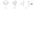
Figure 6: Links of the barycentres of a triangle (a) and an edge (b). The link of the midpoint of an edge is the double cone on the link in a cross-section (c).

Now, to get ${\rm lk}_{X}(\pi(q))$ we must glue together the links of the various points identified to $q$. Using Fig. 6 (a) we note that each glueing identifies a (lower or upper) triangular hemisphere to another one. As we proceed with the glueings, we still have a ball $D^{3}$ whose boundary is given by the union of two triangular hemispheres, until the upper and lower hemisphere are glued together. Such a glueing is determined by a permutation of the vertices of the triangle, and the result is $S^{3}$ if the permutation is the identity, it is the lens space $L_{3,1}$ if the permutation is even but non-trivial, and it is not a $3$-manifold if the permutation is odd (of the three vertices, one is fixed by the permutation, and it is easy to see that its link is the projective plane). Since the triangle glueings are precisely those induced by the face-pairings ${\cal P}$, we have following definition and result:

1. The following should happen for all triangles $(v_{0},v_{1},v_{2})$. Let $v_{3},v_{4}$ be the other vertices of the same $4$-simplex. Let $(v_{0},v_{1},v_{2},v_{4})$ be glued to $(v_{0}^{\prime},v_{1}^{\prime},v_{2}^{\prime},v_{3}^{\prime})$, in this order. Let $v_{4}^{\prime}$ be the other vertex of the same $4$-simplex, and proceed until a glueing of $(v^{(k)}_{0},v^{(k)}_{1},v^{(k)}_{2},v^{(k)}_{4})$ with $(v_{\sigma(0)},v_{\sigma(1)},v_{\sigma(2)},v_{3})$ is first found, where $\{\sigma(0),\sigma(1),\sigma(2)\}=\{0,1,2\}$. Then we should have $\sigma={\rm id}$.

(Here the name Cycl comes from the fact that we look at simplices Cyclically arranged around a codimension-2 face.)

Proposition 4.10

Cycl holds if and only if ${\rm lk}_{X}(\pi(q))\cong S^{3}$ for all barycentres $q$ of triangles.

Note that condition Cycl as stated only makes sense in dimension 4, but one can easily devise an extension to all dimensions. In particular, the $3$-dimensional analogue of Cycl is condition Dir discussed above.

We turn now to codimension 3, so we consider the midpoint $q$ of an edge of $\Delta_{i}$. We arbitrarily choose two points $q_{\pm}$ on the same edge but on opposite sides of $q$, and we note that ${\rm lk}_{X}(q)$ can be naturally identified with the ‘join’ of $\{q_{+},q_{-}\}$ with ${\rm lk}_{\Delta_{i}\cap P}(q)$, where $P$ is a hyperplane through $q$, orthogonal to the edge containing $q$. The notion of ‘join’ $A\vee B$ of two polyhedra $A$ and $B$ is another general one from PL topology, but in the special case where $A$ consists of two points $\{q_{+},q_{-}\}$, the space $\{q_{+},q_{-}\}\vee B$ is simply the union of the two cones $\{q_{+}\}\vee B$ and $\{q_{-}\}\vee B$ glued along the common basis $B$. The link of $q$ in $\Delta_{i}$ is shown in Fig. 6 (b), and the explanation of why it can be described like this is suggested in Fig. 6 (c).

Now, as above, ${\rm lk}_{X}(\pi(q))$ is obtained by glueing together the faces of the various ${\rm lk}_{\Delta_{i^{\prime}}}(q^{\prime})$, where $\pi(q^{\prime})=\pi(q)$. Each face of ${\rm lk}_{\Delta_{i^{\prime}}}(q^{\prime})$ is given by $\{q^{\prime}_{+},q^{\prime}_{-}\}\vee e^{\prime}$, where $e^{\prime}$ is an edge of the triangle ${\rm lk}_{\Delta_{i^{\prime}}\cap P^{\prime}}(q^{\prime})$. Every glueing between ${\rm lk}_{\Delta_{i^{\prime}}}(q^{\prime})=\{q^{\prime}_{+},q^{\prime}_{-}\}\vee e^{\prime}$ and ${\rm lk}_{\Delta_{i^{\prime\prime}}}(q^{\prime\prime})=\{q^{\prime\prime}_{+},q^{\prime\prime}_{-}\}\vee e^{\prime\prime}$ maps $\{q^{\prime}_{+},q^{\prime}_{-}\}$ to $\{q^{\prime\prime}_{+},q^{\prime\prime}_{-}\}$ and $e^{\prime}$ to $e^{\prime\prime}$, and it is determined by these data. The resulting space is then determined by the answers to the following questions:

1. Can the arbitrary $q_{+}/q_{-}$ choice be made in such a way that each $q^{\prime}_{+}$ is glued to a $q^{\prime\prime}_{+}$?

2. What surface results from the triangles ${\rm lk}_{\Delta_{i^{\prime}}\cap P^{\prime}}(q^{\prime})$ under the edge glueings $e^{\prime}\to e^{\prime\prime}$?

Of course the answer to (1) is positive if an only if Dir holds. To answer (2) we first formalize the construction of the surface.

1. Associate to each edge $(v_{0},v_{1})$ of a $4$-simplex $(v_{0},v_{1},v_{2},v_{3},v_{4})$ an abstract triangle $T(v_{0},v_{1})$. The edge is not oriented, so $T(v_{0},v_{1})=T(v_{1},v_{0})$. Denote the vertices of $T(v_{0},v_{1})$ by $T^{v_{j}}(v_{0},v_{1})$, for $j=2,3,4$. For each pairing $(v_{0},v_{1},v_{2},v_{3})\to(v^{\prime}_{0},v^{\prime}_{1},v^{\prime}_{2},v^{\prime}_{3})$, consider the edge-pairings

   $$(T^{v_{i}}(v_{j},v_{k}),T^{v_{l}}(v_{j},v_{k}))\to(T^{v^{\prime}_{i}}(v^{\prime}_{j},v^{\prime}_{k}),T^{v^{\prime}_{l}}(v^{\prime}_{j},v^{\prime}_{k})),\qquad{\rm where}\ \{i,j,k,l\}=\{0,1,2,3\}.$$

   The closed surface $\Sigma({\cal S},{\cal P})$ resulting from these edge-pairings between the triangles should be a union of components homeomorphic to $S^{2}$.

(Here Surf stands for Surface.)

Remark 4.11

1. Each $4$-simplex determines 10 triangles, and each face-pairing between $4$-simplices determines 6 edge-pairings between triangles.

2. Since $\Sigma({\cal S},{\cal P})$ is intrinsically defined as a triangulated surface, one can algorithmically check that a certain component $\Sigma_{0}$ is $S^{2}$, by checking whether $\chi(\Sigma_{0})=2$.

Proposition 4.12

Dir and Surf jointly hold if and only if ${\rm lk}_{X}(\pi(q))\cong S^{3}$ for all midpoints $q$ of edges.

Proof of  4.12. If $q$ is the midpoint of $(v_{0},v_{1})$ then ${\rm lk}_{\Delta_{i}}(q)=\{q_{+},q_{-}\}\vee T(v_{0},v_{1})$, and the labels $T^{v_{i}}(v_{j},v_{k})$ are chosen so that the glueings induced by ${\cal P}$ are precisely those described in Surf. If Dir and Surf hold we deduce that ${\rm lk}_{X}(\pi(q))\cong\{q_{+},q_{-}\}\vee S^{2}\cong S^{3}$. Assume now that ${\rm lk}_{X}(\pi(q))\cong S^{3}$. A closed surface embedded in $S^{3}$ is necessarily orientable, and hence transversely orientable. This implies that we can make a consistent choice of $q_{+}/q_{-}$, so Dir holds. Therefore $S^{3}$ is realized as $\{q_{+},q_{-}\}\vee\Sigma_{0}$ for a component $\Sigma_{0}$ of $\Sigma_{0}({\cal S},{\cal P})$. The link of $q_{+}$ in $\{q_{+},q_{-}\}\vee\Sigma_{0}$ is precisely $\Sigma_{0}$, so $\Sigma_{0}\cong S^{2}$.  4.12

We can now state our main result (see below for a formal proof):

Theorem 4.13

$X^{*}$ is a $4$-manifold if and only if conditions Cycl, Dir and Surf hold.

Remark 4.14

This result implies that it is very easy to check algorithmically whether $X^{\partial}$ is a $4$-manifold with boundary or not. It is also easy to give a presentation of $\partial X^{\partial}$ as a triangulated $3$-manifold, but the triangulation which arises is arbitrarily complicated, so the problem of recognizing whether it is a union of $S^{3}$’s is theoretically solved by the Rubinstein-Thompson [14] algorithm, but undoable in practice. This shows that the best one can really do, using current knowledge, about Questions 4.1-4.3, is the closed $3$-dimensional case and the bounded $4$-dimensional case.

Orientation in dimension 4

Recall that, in dimension 3, condition Ori implies condition Dir. The situation in dimension 4 is more elaborate.

Proposition 4.15

Assume $n=4$. If Ori holds then the permutation $\sigma\in{\hbox{\Got S}}_{3}$ which arises in condition Cycl is automatically an even one. Moreover Ori and Surf jointly imply Dir.

Proof of  4.15. The first assertion is easy: all the triangle-pairings along the sequence in Cycl reverse the induced orientation. For the second assertion, we first note that if Ori holds then each link ${\rm lk}_{\Delta_{i}}(q)$ can be oriented as the boundary of the corresponding star, and the pairings between the bigonal faces of the ${\rm lk}_{\Delta_{i}}(q)$’s reverse the induced orientation. Now, if Surf holds, we can choose orientations on the $T(v_{0},v_{1})$’s so that all edge-pairings reverse orientation. Now we can combine the orientations of ${\rm lk}_{\Delta_{i}}(q)$ and $T(v_{0},v_{1})$ to get a consistent choice of $q_{+}/q_{-}$, so Dir holds.  4.15

It is a tedious exercise, which we omit, to show that these are the only relations which hold in general between the various conditions considered.

Final proofs

The discussion accompanying the introduction of the various conditions almost but not quite proves our main result. We complete its proof now.

Proof of  4.13. By Propositions 4.10 and 4.12, if $X^{*}$ is a $4$-manifold then Cycl, Dir and Surf hold. To see the opposite implication we must show that links of all points, not only of barycentres, are homeomorphic to $S^{3}$. Now condition Cycl implies that the projection $\pi$ is injective on the interior of each triangular face. It follows that our description of ${\rm lk}_{X}(\pi(q))$ extends verbatim from the centre of a triangle to any point in the interior of the same triangle. The same argument applies to edges, because Dir implies that $\pi$ is injective on their interior.  4.13

We conclude this section with a proof omitted above. Here $n$ is again arbitrary.

Proof of  4.6. For (1), we note that $X^{*}$ may be equivalently defined by removing from $X$ not just the vertices but also their closed stars in the second barycentric subdivision. So $X^{*}$ naturally embeds in $X^{\partial}$, and it is clear that if $X^{\partial}$ is manifold then $X^{*}=X^{\partial}\setminus\partial X^{\partial}$ is a manifold.

To conclude (1), we are left to show that if $X^{*}$ is a manifold then $X^{\partial}$ is. Of course we only need to examine links of points of the candidate boundary, i.e. points in the projection of the bases of the stars removed from the $\Delta_{i}$’s. Let $p$ be such a point and consider $q\in\pi^{-1}(p)$. Note that $q$ lies in the link of a vertex $v$ of one of the $\Delta_{i}$’s. Consider now the line in $\Delta_{i}$ through $v$ and $q$, and choose on it points $q_{\pm}$ near $q$ so that $q_{-},q,q_{+},v$ appear in this order on the line. Let $P$ be the hyperplane in $\Delta_{i}$ orthogonal to the line. Then

$${\rm lk}_{\Delta_{i}}(q)=\{q_{+},q_{-}\}\vee{\rm lk}_{P\cap\Delta_{i}}(q),\qquad{\rm lk}_{\Delta^{\partial}_{i}}(q)=\{q_{-}\}\vee{\rm lk}_{P\cap\Delta_{i}}(q).$$

When we consider the glueings ${\cal P}$, we see that all the $q_{-}$’s corresponding to the various $q$’s in $\pi^{-1}(p)$ get identified to a certain point $p_{-}\in X^{\partial}$, while the $q_{+}$’s get identified to a point $p_{+}\in X^{*}\setminus X^{\partial}$. In the meantime the various ${\rm lk}_{P\cap\Delta_{i}}(q)$’s get glued together, yielding a certain polyhedron $W_{p}$. This shows that

$${\rm lk}_{X^{*}}(p)=\{p_{+},p_{-}\}\vee W_{p},\qquad{\rm lk}_{X^{\partial}}(p)=\{p_{-}\}\vee W_{p}.$$

Now, the assumption that $X^{*}$ is a manifold guarantees that ${\rm lk}_{X^{*}}(p)$ is $S^{n-1}$. But the link of $p_{+}$ in $\{p_{+},p_{-}\}\vee W_{p}$ is $W_{p}$, and $S^{n-1}$ is a manifold, so $W_{p}$ is $S^{n-2}$. Then $\{p_{-}\}\vee W_{p}$ is $D^{n-1}$, and the proof of (1) is complete.

To prove (2), note that if $X$ is a manifold then $X^{*}$ is, because it is an open subset of $X$. So, by (1), we see that $X^{\partial}$ is a manifold. So we can assume in any case that $X^{\partial}$ is a manifold. Now $X$ is obtained from $X^{\partial}$ by attaching to each component of $\partial X^{\partial}$ the cone based on the component, and the conclusion easily follows.  4.6

5 Graphic translation of conditions

We describe in this section the combinatorial counterparts in $\textsf{FG}_{4}$ of the conditions Ori, Dir, Surf, and Cycl introduced above. We only provide quick statements and we omit the proofs (except for some hints concerning Surf). One basically only needs to plug the definitions of Section 4 into the construction described in Section 3.

Condition Ori is of course just the condition that the fat graph should be equivalent, with respect to the relation defined at the end of Section 3, to one of $\textsf{FG}_{4}^{+}$. An easy criterion goes as follows: Ori holds if an only we can attach a sign $\epsilon(v)$ to each vertex $v$ of the graph, in such a way that the parity of the permutation attached to any edge is precisely the product of the signs attached to the ends of that edge.

To translate condition Dir, recall from (23) that the four strands leaving a vertex $v$ from a branch $\theta(p_{i_{0}}(v))$ are numbered by $\{0,1,2,3,4\}\setminus\{i_{0}\}$. Moreover a propagator matches such a quadruple of indices with another one, belonging to the same or to another vertex. We now pick $i_{1},i_{2}\in\{0,1,2,3,4\}\setminus\{i_{0}\}$ and arbitrarily declare that $p_{i_{1}}(v)\prec p_{i_{2}}(v)$. Note now that $\{i_{1},i_{2}\}$ appears precisely in three of the branches leaving $v$. We then extend the ordering $\prec$ to the three other pairs matched to $\{p_{i_{1}}(v),p_{i_{2}}(v)\}$ by the propagators, and we continue in a similar way until either a contradiction to $\prec$ is reached or all matching pairs have been visited. Condition Dir si now the condition that no contradiction is ever reached, for any initial choice of $v$ and $i_{1},i_{2}$.

We illustrate the procedure to check Dir with an example. Consider the fat graph of Fig. 7,

Figure 7: A fat graph and the corresponding propagators with canonical labels

let $v$ and $\bar{v}$ be its vertices, and set $i=p_{i}(v)$, $\bar{i}=p_{i}(\bar{v})$ by simplicity. Start for instance by declaring that $3\prec 4$. Extending this relation through the edges labeled $(1\;2)$, id, and $(1\;2\;3)$ we respectively deduce that $\bar{0}\prec\bar{2}$, $\bar{4}\prec\bar{0}$ and $2\prec 4$. Now for each of these pairs we have to follow two edges (not three, because with the third one we would get back to $3\prec 4$), and proceed so forth. Following the inverse of the edge labeled $(2\;4)$ from $\bar{0}\prec\bar{2}$ we deduce that $\bar{3}\prec\bar{4}$, and then following the same edge again we deduce that $\bar{2}\prec\bar{1}$, whereas following the edge labeled $(1\;2)$ from $2\prec 4$ we deduce that $\bar{1}\prec\bar{2}$. So we have a contradiction, and Dir does not hold in this case.

Condition Cycl involves the pattern of circuits already mentioned in Remark 3.2, and obtained by joining the vertices (Fig. 3-centre) with the propagators (Fig. 3-left). To translate Cycl we pick one of these circuits with an arbitrary direction, and we follow the circuit starting from one of the vertex-propagator junctions. We give arbitrary labels $\alpha,\beta,\gamma$ to the three other strands at the same junction, and we follow the labeling as we travel along the circuit, according to the following rules. First, when we travel through a propagator, we give matching strands the same label. Second, when we travel through a vertex, referring to Fig. 3-centre, we note that the various strands come in groups of four, and we examine the relative position of the strand at which the circuit enters the vertex. If this position is the $i$-th one, then the circuit exits at the $(4-i)$-th position, and the labeling rules are as follows: $[\,|\,,\alpha,\beta,\gamma]\leftrightarrow[\alpha,\beta,\gamma,\,|\,]$ and $[\alpha,\beta,\,|\,,\gamma]\leftrightarrow[\gamma,\,|\,,\alpha,\beta]$, where the vertical segment $|$ represents the strand of circuit we are following. The condition is now that, when we come back to the starting junction, the labeling of the three other strands should be the same as at the beginning. Some attention should be paid when a circuit travels more than once through a junction, but the same formal rules actually apply, one should just locally ignore that other strands are globally part of the same circuit.

We use again the same example considered above to illustrate the procedure for checking Cycl. Figure 8

Figure 8: Circuits determined by a fat graph, and labels along one of them

shows the pattern of circuits and highlights one of them. We follow the five edges of this circuit as suggested in the figure, starting with labels $\alpha_{1},\beta_{1},\gamma_{1}$, denoting by $\alpha_{i}^{\prime},\beta_{i}^{\prime},\gamma_{i}^{\prime}$ the labels after the $i$-th edge, and by $\alpha_{i+1},\beta_{i+1},\gamma_{i+1}$ the new labels after going through a vertex. Since when we get back to the beginning of the circuit labels are changed, Cycl does not hold in this case.

We are left to translate condition Surf. Recall that we have to show that a certain triangulated surface $\Sigma$ is the union of components homeomorphic to the sphere. This can be checked by first computing the number $k$ of components, and then by checking that $\chi(\Sigma)=2k$. To compute $k$ we will use the fact that it equals the number of components of the 1-skeleton of the cellularization dual to the triangulation. To check that $\chi(\Sigma)=2k$ we note that if the fat graph has $h$ vertices, then in the triangulation of $\Sigma$ there are $10h$ triangles and $15h$ edges, so we only need to compute the number $m$ of vertices of $\Sigma$ and check that $m=5h+2k$. Summing up, we can express Surf in the following purely combinatorial terms. Consider first the rules of Fig. 9,

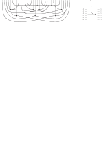
Figure 9: Combinatorial description of the 1-skeleton dual to the triangulation of $\Sigma$.

which allow to associate to the fat graph a trivalent graph. Here the rule for the vertex is explicitly shown, and the rule for the edge is that the strand labeled $\{i,j\}$ on the right should be matched with the strand labeled $\varphi_{\sigma}(\{i,j\})$ on the left, where $\varphi_{\sigma}(\{i,j\})=\{\tau(i),\tau(j)\}$, and $\tau=\sigma\circ(1\;4)$. Denote by $k$ the number of trivalent graphs in this picture. Next consider the rules of Fig. 10,

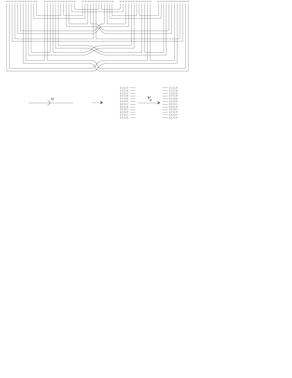
Figure 10: Circuits corresponding to the vertices of the triangulation of $\Sigma$.

where the meaning is as above, with $\psi_{\sigma}(\{i,j\},k)=(\{\tau(i),\tau(j)\},\tau(k))$, $\tau=\sigma\circ(1\;4)$. Denote by $m$ the number of circuits in this figure. Then Surf is precisely the condition that $m-2k$ is 5 times the number of vertices of the fat graph.

Remark 5.1

It is actually possible to attach colours in ${\hbox{\Got S}}_{2}$ to the edges of the trivalent graph of Fig. 9, turning it into a fat $2$-graph, in such a way that the circuits of Fig. 10 are precisely those defined by this graph as explained in Remark 3.2. We have refrained from doing this and preferred to give an explicit rule.

——————————–

We thank Mauro Carfora, Annalisa Marzuoli, Carlo Rovelli and Gianni Cicuta for discussions and correspondence.

References

- [1] For an overview on current attempts towards a quantum theory of gravity see: “Special Issue on Quantum Geometry and Diffeomorphism Invariant Quantum Field Theory,” J. Math. Phys. 36, 6069-6547 (1995).
- [2] F. David, Nucl. Phys. B257, 45 (1985). J. Ambjorn, B. Durhuus, J. Frolich, Nucl. Phys. B257, 433 (1985). V. A. Kazakov, I. K. Kostov, A. A. Migdal, Phys. Lett. 157, 295 (1985). D. V. Boulatov, V. A. Kazakov, I. K. Kostov, A. A. Migdal, Nucl. Phys. B275, 641 (1986). M. Douglas, S. Shenker, Nucl. Phys. B335, 635 (1990). D. Gross, A. Migdal, Phys. Rev. Lett. 64, 635 (1990); E. Brezin, V. A. Kazakov, Phys. Lett. B236, 144 (1990).
- [3] J. Ambjorn, M. Carfora, A. Marzuoli, “The Geometry of Dynamical Triangulations,” Lecture Notes in Physics Vol. m50, Springer-Verlag, Berlin, 1997.
- [4] N. Sasakura, Mod. Phys. Lett. A6, 2613 (1991).
- [5] M. Gross, Nucl. Phys. Proc. Suppl. 25A, 144-149 (1992).
- [6] D. V. Boulatov, Mod. Phys. Lett. A7 (1992), 1629; Int. J. Mod. Phys. A8 (1993), 3139-3162.
- [7] H. Ooguri, Mod. Phys. Lett. A7, 2799 (1992).
- [8] R. De Pietri, L. Freidel, K. Krasnov, C. Rovelli, “Barrett-Crane model from a Boulatov-Ooguri field theory over a homogeneous space,” Nucl. Phys. B (2000), to appear. e-Print Archive: hep-th/9907154.
- [9] G. Ponzano, T. Regge, in Spectroscopy and group theoretical methods in Physics, edited by F. Bloch (North-Holland, Amsterdam, 1968). V. G. Turaev, O. Y. Viro, Topology 31, 865–902 (1992).
- [10] J. W. Barrett, L. Crane, J. Math. Phys. 39, 3296 (1998).
- [11] M. Reisenberger, “Worldsheet formulations of gauge theories and gravity,” talk given at the 7th Marcel Grossmann Meeting, Stanford, July 1994, e-Print Archive: gr-qc/9412035. J. Baez, Class. Quant. Grav. 15, 1827 (1998). M. P. Reisenberger, C. Rovelli, Phys. Rev. D56 3490 (1997); R. De Pietri, “Canonical loop quantum gravity and spin foam models,” to appear in the proceedings of the XXIII Congress of the Italian Society for General Relativity and Gravitational Physics (SIGRAV), 1998, e-Print Archive: gr-qc/9903076. M. P. Reisenberger, C. Rovelli, “Space-Time as a Feynman Diagram: the Connection Formulation,” e-Print Archive: gr-qc/0002095; “Spin Foams As Feynman Diagrams,” e-Print Archive: gr-qc/0002083.
- [12] B. Rourke, B. Sanderson, “An Introduction to Piecewise Linear Topology,” Ergebn. Math. Wiss. Vol. 69, Springer-Verlag, Berlin-Heidelberg-New York, 1972.
- [13] R. Benedetti, C. Petronio, Manuscripta Math. 88, 291-310 (1995).
- [14] H. Rubinstein, “An algorithm to recognize the -sphere,” Proceedings of the International Congress of Mathematicians, Vol. 1, 2 (Zürich, 1994), 601–611, Birkhäuser, Basel, 1995. A. Thompson, “Thin position and the recognition problem for ,” Math. Res. Lett. 1, 613–630 (1994).