IS OUR VACUUM STABLE ?

Abstract

The stability of our vacuum is analyzed and several aspects concerning this question are reviewed. 1) In the standard Glashow-Weinberg-Salam (GWS) model we review the instability towards the formation of a bubble of lower energy density and how the rate of such bubble formation process compares with the age of the Universe for the known values of the GWS model. 2) We also review the recent work by one of us (E.I.G) concerning the vacuum instability question in the context of a model that solves the cosmological constant problem. It turns out that in such model the same physics that solves the cosmological constant problem makes the vacuum stable. 3) We review our recent work concerning the instability of elementary particle embedded in our vacuum, towards the formation of an infinite Universe. Such process is not catastrophic. It leads to a ”bifurcation type” instability in which our Universe is not eaten by a bubble (instead a baby universe is born). This universe does not replace our Universe rather it disconnects from it (via a wormhole) after formation.

1 On Vacuum Stability in the Weinberg-Salam model.

In modern theories of elementary particle interactions, the vacuum is defined by the expectation value of a scalar field. In the Weinberg-Salam[1] model such scalar field (the Higgs field) is responsible for the gauge symmetry breaking and fermion masses production. Let us begin our studies of vacuum instability by considering a model containing just a scalar field with a potential $V(\phi)$ as depicted in fig 1.

Figure 1: Scalar Field Potential with an Unstable Vacuum

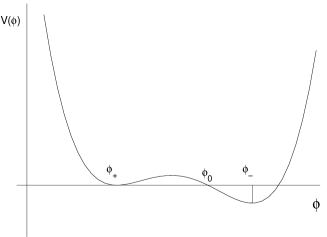
The theory is governed by an action in the form $S=\int d^{4}x(\frac{1}{2}\partial_{\mu}\phi\partial^{\mu}\phi-V(\phi))$, where $\partial_{\mu}\phi\partial^{\mu}\phi=(\partial_{0})^{2}-(\nabla\phi)^{2}$

As it is obvious, there is no classical (in Minkowski space) solution connecting $\phi_{+}$ and $\phi_{-}$. There is however a Euclidean solution connecting a point close to $\phi_{-}$ to $\phi_{+}$, the tunneling solution. This is a solution in imaginary time. Defining $\tau=it$, $\rho=\sqrt{\vec{x}^{2}+\rho^{2}}$ and considering solutions of the form $\phi=\phi(\rho)$, we obtain the following equation of motion

$$\frac{d^{2}\phi}{d\rho^{2}}+\frac{3}{\rho}\frac{d\phi}{d\rho}+V^{{}^{\prime}}(\phi)=0$$ (1)

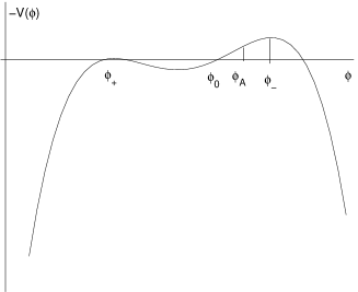
Equation (1) is like that of a particle, $\phi$ playing the role of ”position”, $\rho$ ”time”, $\frac{3}{\rho}\frac{d\phi}{d\rho}$ friction, $-V$, the mechanical potential (see$-V$ in Fig.2).

Figure 2: The Effective Mechanical Potential

To avoid a singularity at $\rho=0$, $\frac{d\phi}{d\rho}$ must vanish for $\rho=0$. If we set as initial condition at $\rho=0$, $\phi$ close to $\phi=\phi_{-}$ the field stays close to $\phi=\phi_{-}$ for a long $\rho$ interval, the friction term becomes negligible and $\phi$ arrives at $\phi=\phi_{+}$ with $\frac{d\phi}{d\rho}\neq 0$, i.e. ”overshoots”. If $\phi=\phi_{0}$, because of the friction the field does not make it to $\phi=\phi_{+}$. By continuity of a value $\phi=\phi_{A}$ exists such that $\phi\rightarrow\phi_{+}$ as $\rho\rightarrow\infty$. This is the tunneling solution. This solution has a classical Euclidean action $S_{E}$ and the tunneling probability per unit time per unit volume is proportional to $e^{-S_{E}}$. $\phi_{A}\rightarrow\phi_{-}$ takes place classically.
In the quantum theory one finds zero-point fluctuations that give rise to vacuum energy $\frac{1}{2}\hbar\omega$ for each boson mode $(\omega=\sqrt{\vec{p}^{2}+m^{2}})$, since masses depend on the Higgs field ($m^{2}=V^{"}(\phi)$ for the Higgs field itself, $m^{2}\sim e^{2}\phi^{2}$ for gauge vector fields, etc.) and $\frac{1}{2}\Sigma\hbar\omega\rightarrow\frac{1}{2}V\int\frac{d^{3}k}{(2\pi)^{3}}\hbar\sqrt{\vec{k}^{2}+m^{2}(\phi)}$, we see that an infinite $\phi$ dependent vacuum energy appears. The Dirac fermions also contribute $-\hbar\omega$ for each occupied negative energy state. The resulting energy density $V_{eff}(\phi)$ makes sense after a renormalization process which get rid of the infinities. The process of renormalization introduces an arbitrary scale into the problem. If we demand that such scale will not affect physical quantities like $V_{eff}(\phi)$ itself, we arrive at what is called renormalization group equation for $V_{eff}(\phi)$. Such $V_{eff}(\phi)$ holds for small coupling although $\phi$ itself can be large.
One can then ask: for which values $V_{eff}(\phi)$ our vacuum is unstable? One can check that for the known values of $m_{Higgs}>90Gev$,$V_{eff}(\phi=0)>V_{eff}(\phi_{+})$ ($\phi_{+}$ is the value of the Higgs for our vacuum), but for large values of $\phi$, $V_{eff}(\phi)$ can be negative (conventionally we set $V_{eff}(\phi_{+})\equiv 0$). The condition that does not happen gives[2] $m_{top}\leq 95Gev+0.60m_{Higgs}$

Notice that for $m_{top}\approx 175Gev$, this implies that $m_{Higgs}\geq 135Gev$, while the experimental data only tell us that $95Gev\leq m_{Higgs}\leq 190Gev$. So that we cannot tell for sure whether the standard model predicts a stable or unstable vacuum.
Even assuming the vacuum is unstable, which is possible according to what we have seen before, can ask: was the age of the universe long enough so that the probability of some nucleation took place in our past light cone? The space-time volume of our past light cone $\sim t^{4}$, $t$ is the age of the universe and the probability of nucleating per unit time per unit volume $\sim e^{-S_{E}}$. 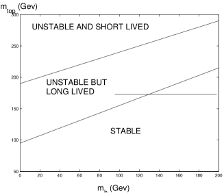The probability of nucleation is $\sim t^{4}e^{-S_{E}}$ and the age of the universe in electroweak units is $t\sim e^{101}$ so that $t^{4}e^{-S_{E}}\sim e^{-S_{E}+404}$. So that $S_{E}\geq 404$ gives the middle region Fig. 3 where the rate is not high enough so it is unlikely that we noticed already any phase transition.
The value $S_{E}\geq 404$ is consistent with the known bounds on $m_{H}$ and the known value of $m_{top}$ (See Fig. 3 which contains the inserted horizontal line $m_{top}=175Gev,90Gev<m_{H}<190Gev$) .

Figure 3: Regions of Stability and Unstability

2 The Cosmological Constant Problem

Calculations of $V_{eff}(\phi)$ are generally a calculation of the vacuum energy of the universe and how it depends on $\phi$. In flat space there is no meaning to the constant part of $V_{eff}(\phi)$ if gravity is ignored. Once gravity taken into account is very important. The naive prediction for $V_{eff}(\phi)|_{\phi=\phi_{min}}=\infty$ but we really need $V_{eff}(\phi)|_{\phi=\phi_{min}}=0$.

One has the suspicion that the calculations of $V_{eff}(\phi)$ mentioned above may miss some physics. Fine tuning $V_{eff}(\phi)$, by adding a constant so that $V_{eff}(\phi)=0$ may not be enough as we will argue, since the physics that sets $V_{eff}(\phi_{+})\approx 0$ can act again when $V_{eff}$ ”tries” to cross once again the zero value and this could affect seriously our notions concerning stability of the vacuum.

3 A Model that sets $V_{eff}(\phi_{+})=0$ naturally

Observation: Usually Generally Covariant theory is build from the action $S=\int L\sqrt{-g}d^{4}x$, $g=det(g_{\mu\nu})$, $L=scalar$, ($L^{\prime}=L$ under general coordinate transformations). Notice that $\sqrt{-g}d^{4}x$ is an invariant volume element. It is possible to build another volume element, independent of $g_{\mu\nu}$. Take for example, given 4-scalars $\varphi_{a}$ (a = 1,2,3,4), the density

$$\Phi=\varepsilon^{\mu\nu\alpha\beta}\varepsilon_{abcd}\partial_{\mu}\varphi_{a}\partial_{\nu}\varphi_{b}\partial_{\alpha}\varphi_{c}\partial_{\beta}\varphi_{d}$$ (2)

$\Phi$ transform like $\sqrt{-g}$, so $\Phi d^{4}x$ is also an invariant.

One can allow both geometrical objects to enter the theory and consider[3]

$$S=\int L_{1}\Phi d^{4}x+\int L_{2}\sqrt{-g}d^{4}x$$ (3)

Here $L_{1}$ and $L_{2}$ are $\varphi_{a}$ independent. There is a good reason not to consider mixing of $\Phi$ and $\sqrt{-g}$ , like for example using $\frac{\Phi^{2}}{\sqrt{-g}}$. This is because (3) is invariant (up to the integral of a total divergence) under the infinite dimensional symmetry $\varphi_{a}\rightarrow\varphi_{a}+f_{a}(L_{1})$ where $f_{a}(L_{1})$ is an arbitrary function of $L_{1}$ if $L_{1}$ and $L_{2}$ are $\varphi_{a}$ independent. Such symmetry (up to the integral of a total divergence) is absent if mixed terms are present.

We will study now the dynamics of a scalar field $\phi$ interacting with gravity as given by the action (3) with[4]

$$L_{1}=\frac{-1}{\kappa}R(\Gamma,g)+\frac{1}{2}g^{\mu\nu}\partial_{\mu}\phi\partial_{\nu}\phi-V(\phi),L_{2}=U(\phi)$$ (4)

$$R(\Gamma,g)=g^{\mu\nu}R_{\mu\nu}(\Gamma),R_{\mu\nu}(\Gamma)=R^{\lambda}_{\mu\nu\lambda},R^{\lambda}_{\mu\nu\sigma}(\Gamma)=\Gamma^{\lambda}_{\mu\nu,\sigma}-\Gamma^{\lambda}_{\mu\sigma,\nu}+\Gamma^{\lambda}_{\alpha\sigma}\Gamma^{\alpha}_{\mu\nu}-\Gamma^{\lambda}_{\alpha\nu}\Gamma^{\alpha}_{\mu\sigma}.$$ (5)

In the variational principle $\Gamma^{\lambda}_{\mu\nu},g_{\mu\nu}$, the scalar fields $\varphi_{a}$ and the scalar field $\phi$ are to be treated as independent variables.

We can require the scale invariance of the theory. If we perform the global scale transformation ($\theta$ = constant) $g_{\mu\nu}\rightarrow e^{\theta}g_{\mu\nu}$ then (2), with the definitions (3), (4), is invariant. $V(\phi)$ and $U(\phi)$ are in the form $V(\phi)=f_{1}e^{\alpha\phi},U(\phi)=f_{2}e^{2\alpha\phi}$ and $\varphi_{a}$ is transformed according to $\varphi_{a}\rightarrow\lambda_{a}\varphi_{a}$ (no sum on a) which means $\Phi\rightarrow\biggl{(}\prod_{a}{\lambda}_{a}\biggr{)}\Phi\equiv\lambda\Phi$ such that $\lambda=e^{\theta}$ and $\phi\rightarrow\phi-\frac{\theta}{\alpha}$. In this case we call the scalar field $\phi$ needed to implement the scale invariance as ”dilaton”.

Now,in the general case, let us consider the equations which are obtained from the variation of the $\varphi_{a}$ fields. We obtain then $A^{\mu}_{a}\partial_{\mu}L_{1}=0$ where $A^{\mu}_{a}=\varepsilon^{\mu\nu\alpha\beta}\varepsilon_{abcd}\partial_{\nu}\varphi_{b}\partial_{\alpha}\varphi_{c}\partial_{\beta}\varphi_{d}$. Since det $(A^{\mu}_{a})=\frac{4^{-4}}{4!}\Phi^{3}\neq 0$ if $\Phi\neq 0$. Therefore if $\Phi\neq 0$ we obtain that $\partial_{\mu}L_{1}=0$, or that $L_{1}=M$, where M is constant. This constant M appears in a self-consistency condition of the equations of motion that allows us to solve for $\chi\equiv\frac{\Phi}{\sqrt{-g}}$

$$\chi=\frac{2U(\phi)}{M+V(\phi)}.$$ (6)

To get the physical content of the theory, it is convenient to go to the Einstein conformal frame where

$$\overline{g}_{\mu\nu}=\chi g_{\mu\nu}$$ (7)

and $\chi$ given by (6). In terms of $\overline{g}_{\mu\nu}$ the non Riemannian contribution (defined as $\Sigma^{\lambda}_{\mu\nu}=\Gamma^{\lambda}_{\mu\nu}-\{^{\lambda}_{\mu\nu}\}$ where $\{^{\lambda}_{\mu\nu}\}$ is the Christoffel symbol), disappears from the equations, which can be written then in the Einstein form ($R_{\mu\nu}(\overline{g}_{\alpha\beta})$ = usual Ricci tensor)

$$R_{\mu\nu}(\overline{g}_{\alpha\beta})-\frac{1}{2}\overline{g}_{\mu\nu}R(\overline{g}_{\alpha\beta})=\frac{\kappa}{2}T^{eff}_{\mu\nu}(\phi)$$ (8)

where

$$T^{eff}_{\mu\nu}(\phi)=\phi_{,\mu}\phi_{,\nu}-\frac{1}{2}\overline{g}_{\mu\nu}\phi_{,\alpha}\phi_{,\beta}\overline{g}^{\alpha\beta}+\overline{g}_{\mu\nu}V_{eff}(\phi),V_{eff}(\phi)=\frac{1}{4U(\phi)}(V+M)^{2}.$$ (9)

If $V(\phi)=f_{1}e^{\alpha\phi}$ and $U(\phi)=f_{2}e^{2\alpha\phi}$ as required by scale invariance, we obtain from (10) $V_{eff}=\frac{1}{4f_{2}}(f_{1}+Me^{-\alpha\phi})^{2}$

Since we can always perform the transformation $\phi\rightarrow-\phi$ we can choose by convention $\alpha>O$. We then see that as $\phi\rightarrow\infty,V_{eff}\rightarrow\frac{f_{1}^{2}}{4f_{2}}=$ const. providing an infinite flat region. Also a minimum is achieved at zero cosmological constant for the case $\frac{f_{1}}{M}<O$ at the point $\phi_{min}=\frac{-1}{\alpha}ln\mid\frac{f_{1}}{M}\mid$. Finally, the second derivative of the potential $V_{eff}$ at the minimum is $V^{\prime\prime}_{eff}=\frac{\alpha^{2}}{2f_{2}}\mid{f_{1}}\mid^{2}>O$ if $f_{2}>O$,

There are many interesting issues that one can raise here. The first one is of course the fact that a realistic scalar field potential, with massive excitations when considering the true vacuum state, is achieved in a way which is consistent with the idea of the scale invariance. The second point to be raised is that since there is an infinite region of flat potential for $\phi\rightarrow\infty$, we expect a slow rolling new inflationary scenario to be viable, provided the universe is started at a sufficiently large value of the scalar field $\phi$. Furthermore, one can consider this model as suitable for the present day universe rather than for the early universe, after we suitably reinterpret the meaning of the scalar field $\phi$. This can provide a long lived almost constant vacuum energy for a long period of time, which can be small if $f_{1}^{2}/4f_{2}$ is small.

Such small energy density will eventually disappear when the universe achieves its true vacuum state.
Notice that for generic functions $V(\phi)$, $U(\phi)$ the minimum of $V_{eff}(\phi)$, as given from (9), is at zero if $V+M=0$ at some point and if $V^{\prime}$ is finite there (also $U>0$ there). So $V^{\prime}_{eff}=0$ and $V_{eff}=0$ is achieved generally without fine tuning! If in the neighborhood of $\phi_{+}$ $V+M=0$, $U(\phi)>0$ and $V+M$ as a function of $\phi$ that goes through zero. Then $V_{eff}\sim\frac{(V+M)^{2}}{4U(\phi_{+})}$ has a local minimum at zero. That is $V(\phi_{+})=0$ and $V(\phi_{+})=0$ automatically without fine tuning. Therefore zero vacuum energy state is obtained naturally!
Going back to the general $V(\phi)$, $U(\phi)$ case we can ask the question: given the classically stable state $\phi_{+}$, where $\phi=\phi_{+}$, $U(\phi_{+})>0$, $V(\phi_{+})+M=0$ can we make this into an unstable state?. Remember that $V_{eff}=\frac{(V+M)^{2}}{4U(\phi_{+})}$ and that we obtained $V+M=0$ as a stable (classically) state under the conditions that $U$ is $>0$ at this point and it is a regular function there. We take to be true that $U(\phi)$ is a nice function everywhere. The only way $V_{eff}=\frac{(V+M)^{2}}{4U}$ can change sign is for $U(\phi)$ to change sign. For $U(\phi)$ being a nice function, this can only happen if $U(\phi)$ goes to zero. If no fine tuning is invoked at that point, $V+M\neq 0$ (if it is true, for other $M$, i.e. for another initial condition of the universe it will not be true). Then $V_{eff}$ looks like in Fig.4

Figure 4: The Effective Potential for the Case $U(\phi)$ contains zero

Remember that in the euclidean solution relevant for nucleation -$V_{eff}$ is the relevant potential.

Figure 5: Effective Mechanical Potential when $U(\phi)$ contains zero

It is clear from Fig.5 that no tunneling is possible now!
From eq.(6) we have $V+M\rightarrow 0\Rightarrow|\Phi|>>\sqrt{-g}$ and $U\rightarrow 0\Rightarrow|\Phi|<<\sqrt{-g}$.
It is interesting to see what the volume element $\sqrt{-\bar{g}}d^{4}x$ where $\bar{g}_{\mu\nu}=\chi g_{\mu\nu}=$ Einstein metric compares with the volume element $\Phi d^{4}x$. Indeed, $\sqrt{-\bar{g}}=\chi^{2}\sqrt{-g}=\chi\Phi$, so that $\sqrt{-\bar{g}}>>|\Phi|$ for $V+M\rightarrow 0$, i.e. Einstein energy density gets diluted $\Rightarrow V_{eff}\rightarrow 0$. On other limit, $U\rightarrow 0$, $\sqrt{-\bar{g}}<<|\Phi|$, implies that Einstein energy density gets concentrated.This is the physical reason that leads to the energy barrier against crossing from $V_{eff}>0$ to $V_{eff}<0$.

4 The Decay of an Elementary Particle into a Universe

Finally we consider a different type of instability of our vacuum. In this case a region which contains a false vacuum inside, like an elementary particle, can decay into a universe!
We considered a model of an elementary particle [5] as a $2+1$ dimensional brane evolving in a $3+1$ dimensional space. The introduction of a gauge field which takes place in the brane as well as a normal surface tension, following the standard approach to the theory of extended objects [6], can lead to a stable ”elementary particle” configuration. The simplest form of the action that permits a stable configuration is:

$$S=\sigma_{0}\int\sqrt{-h}d^{3}y+\lambda\int\sqrt{-h}F_{\alpha\beta}F^{\alpha\beta}d^{3}y$$ (10)

Where $h_{\alpha\beta},\ \alpha\ \beta=0,1,2$ is the induced metric on the surface of the membrane, $h=det(h_{\alpha\ \beta})$, and $F_{\alpha\beta}F^{\alpha\beta}$ the Lagrangian of the gauge field. If we assume a spherically symmetric vector potential in the brane (up to a gauge transformation) of the simplest form (a monopole potential), we receive the general form of the surface tension as; $\sigma=\sigma_{0}+\frac{\sigma_{1}}{r^{4}}$ ($\sigma_{1}$ being $2\lambda f^{2}$, f being the strength of the monopole configuration defined by the vector potential in the brane). The energy of the static wall, $4\pi r^{2}\sigma$, has a non trivial minimum for any $\lambda>0$ that permits a stable configuration. This is the simplest possible model, below we shall consider the effect of gravity and of an internal vacuum energy. A membrane as discussed above, defines boundaries between different phases with different values for their energy densities.

We took the metric for the inside of the membrane phase, a false vacuum one, as a de Sitter metric, i.e., $ds^{2}=-(1-\chi^{2}r^{2})dt^{2}+\frac{dr^{2}}{(1-\chi^{2}r^{2})}+r^{2}(d\theta^{2}+sin^{2}\theta d\phi^{2})$ where $\chi^{2}\ =\ \frac{8\pi\rho G}{3}$, $\rho$ is the energy density. Outside, in the empty space, we can have only a Schwarzschild space time according to Birkhoff’s theorem, i.e., $ds^{2}=-(1-\frac{2GM}{r})dt^{2}+\frac{dr^{2}}{(1-\frac{2GM}{r})}+r^{2}(d\theta^{2}+sin^{2}\theta d\phi^{2})$ and in the membrane, we have a singular energy momentum tensor.
Demanding that Einstein’s equations to be satisfied not only inside and outside but also in the membrane we get [5] $\sqrt{1-\chi^{2}r^{2}+\dot{r}^{2}}-\sqrt{1-\frac{2GM}{r}+\dot{r}^{2}}=4\pi G\sigma r$ where $\dot{r}\equiv\frac{dr}{d\tau}$ and $\sigma$ is the one discussed before. Following (7), we take as the Hamiltonian the mass of the system, which gives us:

$$H=\frac{\chi^{2}r^{3}}{2G}-\frac{(4\pi G)^{2}\sigma^{2}r^{3}}{2G}+4\pi\sigma r^{2}(1-\chi^{2}r^{2}+\dot{r}^{2})^{1/2}$$ (11)

Having obtained the Hamiltonian, all the others classical dynamical variables can be obtained as was done in [7]. The conjugate momentum p will be equal to

$p=\frac{\partial L}{\partial\dot{r}}$, the Lagrangian will be equal to $L=\dot{r}\int H\frac{d\dot{r}}{\dot{r}^{2}}$ This give for the conjugate momentum $p=\int\frac{\partial H}{\partial\dot{r}}\frac{d\dot{r}}{\dot{r}}$ Using H as before we arrive at the value of p, which is equal to $p=4\pi\sigma r^{2}arcsinh(\frac{\dot{r}}{\sqrt{1-\chi^{2}r^{2}}})$ inside horizon and $p=4\pi\sigma r^{2}arccosh(\frac{\dot{r}}{\sqrt{\chi^{2}r^{2}-1}})$ outside. An arbitrary function of r can be added in the definition of p. Classically it corresponds to an additional total derivative of a function of r in the Lagrangian, while in Quantum Mechanics it corresponds to a redefinition of the wavefunction $\Psi^{\prime}=e^{if(r)}\Psi$ This means that the Hamiltonian can be taken as

$$H=\frac{\chi^{2}r^{3}}{2G}-\frac{(4\pi G)^{2}\sigma^{2}r^{3}}{2G}+4\pi\sigma r^{2}\sqrt{1-\chi^{2}r^{2}}K(\frac{p}{4\pi\sigma r^{2}})$$ (12)

where $K=cosh$ inside the horizon and $K=sinh$ outside it. In order to achieve a quantum mechanical approach we shall assume that $p=-i\frac{\partial}{\partial r}$ and from this $e^{-ia\frac{\partial}{\partial r}}\Psi(r)=\Psi(r-ia)$. The Schroedinger equation is $H\Psi=m\Psi$ in which m is the mass parameter of the external Schwarzschild solution. Defining the dimensionless variable (in units where $\hbar$ = c = 1) $x=\frac{4\pi r^{3}\sigma_{0}}{3}-4\pi\frac{\sigma_{1}}{r}$ we receive the following difference equation for $\Psi$, interpreting the order of operators in $\frac{p}{4\pi\sigma r^{2}}$ as $\frac{1}{4\pi\sigma r^{2}}p$ $f(x)\Psi(x)+g(x)[\Psi(x+i)+\Psi(x-i)]=0$ f and g are real functions of x, inside the horizon, and

$$f(x)\Psi(x)+g(x)[\Psi(x+i)-\Psi(x-i)]=0$$ (13)

outside. Expanding the equation for $\Psi$ outside the horizon, taking $x>>1$ (setting $r\ \sim\frac{1}{\chi}$ and $\chi\ \sim\ G^{1/2}\ \rho_{0}^{1/2}$, we see that $x>>1$ is satisfied if the typical energy scales determining $\sigma_{0},\ \sigma_{1}\ and\ \rho_{0}$ are $<<$ Planck scale) and keeping the first nonvanishing contribution only, we receive the equation:

$$-\frac{f}{2g}\Psi(x)=i\frac{\partial\Psi}{\partial x}$$ (14)

It has the form of a Schroedinger equation (x is time-like outside the horizon). The solution is $\Psi=Ce^{i\int(-\frac{f}{2g})dx}$ where C=constant. This means that once a bubble passes the horizon it will expand indefinitely, since $|\Psi|^{2}$ = constant and therefore the modulus of the amplitude for the bubble being at $r=\frac{1}{\chi}+\epsilon$ ($\epsilon>0$ is very small) is the same as the amplitude for the membrane being at r $\rightarrow\ \infty$ with probability equal 1. Therefore if the wave function of the bubble has a tail long enough, so it can get the horizon $r=\frac{1}{\chi}$, we have the possibility of the formation of an infinite size bubble i.e. the formation of a universe. The resulting universe becomes large not by expanding and displacing an exterior region. This cannot do, since the interior has negative pressure and the outside zero pressure. Really the bubble expands forming a wormhole region that disconnects from the outside creating a ”baby” universe in this case[8].

References

- [1] S.Weinberg, Phys. Rev. Lett. 19 (1967) 1264; A.Salam, in Elementary Particle Theory, ed. N.Svartholm (Stockholm (1968)).
- [2] For a review see M.Sher, Phys. Rept. 179 (1989) 273.
- [3] For a review and further references see E.I.Guendelman and A.Kaganovich, Phys. Rev D60 (1999): 065004.
- [4] E.I.Guendelman, Mod. Phys. Lett.A14 (1999) 1043; gr-qc/9901067; E.I.Guendelman, Mod. Phys. Lett.A14 (1999) 1397; E.I.Guendelman, Class. Quant. Grav. 17 (2000) 261.
- [5] E. I. Guendelman and J. Portnoy, Class. Quant. Grav. 16 (1999) 3315.
- [6] Y. Ne’eman, E. Eizenberg, Membranes and Other Extendons, World Scientific, Singapore 1995
- [7] V. A. Berezin Phys. Rev D55 (1997) 2139
- [8] For a review see A. H. Guth, Physica Scripta Nobel Symposium 79, 1991, p.237.