Dynamic Cosmic Strings II: Numerical evolution of excited Cosmic Strings

Abstract

An implicit, fully characteristic, numerical scheme for solving the field equations of a cosmic string coupled to gravity is described. The inclusion of null infinity as part of the numerical grid allows us to apply suitable boundary conditions on the metric and matter fields to suppress unphysical divergent solutions. The code is tested by comparing the results with exact solutions, checking that static cosmic string initial data remain constant when evolved and undertaking a time dependent convergence analysis of the code. It is shown that the code is accurate, stable and exhibits clear second order convergence. The code is used to analyse the interaction between a Weber–Wheeler pulse of gravitational radiation with the string. The interaction causes the string to oscillate at frequencies proportional to the masses of the scalar and vector fields of the string. After the pulse has largely radiated away the string continues to ring but the oscillations slowly decay and eventually the variables return to their static values.

I Introduction

This is the second paper in a series devoted to the study of dynamic cosmic strings. In the previous paper [1], henceforth referred to as paper I, we derived the equations of motion for a time dependent cylindrically symmetric cosmic string coupled to a gravitational field with two degrees of freedom. The treatment involved using a Geroch decomposition to reformulate the problem in terms of matter fields on a $2+1$ dimensional spacetime and two geometrical variables $\nu$ and $\tau$ which describe the gravitational degrees of freedom. Unlike the original cylindrical metric the reduced $2+1$ spacetime is asymptotically flat and this allows us to implement a numerical treatment of the field equations which includes null infinity as part of the grid. In paper I we presented a Cauchy-characteristic matching (CCM) code that reproduced the results of several vacuum solutions with both one and two degrees of freedom but did not perform entirely satisfactorily in the presence of matter. We have therefore developed a second implicit, purely characteristic code. The numerical details, the testing and the convergence analysis of this implicit code will be described in this paper. We also give a detailed analysis of the interaction between the string and a pulse of gravitational radiation.

After briefly describing the variables used for the coupled system in section II the details of the numerical scheme are presented in section III. We begin by describing the relaxation method we use for the much simpler problem of a static cosmic string in Minkowski spacetime and demonstrate how this approach leads naturally to the implicit scheme used to solve the general case of a dynamical cosmic string coupled to gravity. The testing of the code is described in section IV. This involves comparing it with exact solutions, checking that static cosmic string initial data remain static when they are evolved, and undertaking a time dependent convergence analysis of the code. We are able to show that the code is accurate, stable and shows clear second order convergence. In section V we analyse the interaction between an initially static cosmic string and a Weber–Wheeler type pulse of gravitational radiation. We show that this interaction causes the string fields $S$ and $P$ to oscillate and examine how this oscillation depends upon both the width and amplitude of the pulse and also upon the constants $e$, $\lambda$ and $\eta$. The key result is that the frequencies are essentially independent of the nature of the Weber–Wheeler wave but are proportional to the masses $m_{S}$ and $m_{P}$ associated with the scalar field $S$ and the vector field $P$. The string continues to ring after the gravitational pulse has largely radiated away, but the oscillations slowly decay and the variables eventually return to their static values. It is only possible to observe this effect because of the long term stability of the code. Finally in section VI we discuss our results and outline future work.

II The variables and field equations

We begin with a brief summary of the variables used to describe the spacetime and the string. In cylindrical polar coordinates $(t,\rho,\phi,z)$ we may write the line element for a cylindrically symmetric spacetime with two degrees of freedom as a modified version of that given by Jordan, Ehlers, Kundt and Kompaneets [2], [3]

$$ds^{2}=e^{2(\gamma-\psi)}(dt^{2}-d\rho^{2})-\rho^{2}e^{-2\psi}d\phi^{2}-e^{2(\psi+\mu)}(\omega d\phi+dz)^{2},$$ (1)

where $\psi$, $\omega$, $\mu$ and $\gamma$ are functions of $t$, $\rho$. As shown in paper I, in order to work with an asymptotically flat spacetime it is convenient to make a Geroch decomposition [4] in which the 4-dimensional metric is replaced by a 3-dimensional one and two auxiliary scalar fields. These scalar fields are the norm of the axial Killing vector $\nu$ and the Geroch potential $\tau$ and are related to $\psi$ and $\omega$ by equations (15) and (16) of paper I, while the conformal 3-dimensional line element is given by

$$d{\tilde{\sigma}}^{2}=e^{2(\gamma+\mu)}(dt^{2}-d\rho^{2})-\rho^{2}e^{2\mu}d\phi^{2}.$$ (2)

The cosmic string is described by a complex scalar field $\Phi$ coupled to a U(1) gauge field $A_{\mu}$, which in cylindrical symmetry can be written as [1]

$$\Phi = \frac{1}{\sqrt{2}}S(t,\rho)e^{i\phi},$$ (3)

$$A_{\mu} = \frac{1}{e}[P(t,\rho)-1]\nabla_{\mu}\phi.$$ (4)

It is also helpful to introduce rescaled coupling constants and variables given by

$$X = \frac{S}{\eta},$$ (5)

$$\alpha = \frac{e^{2}}{\lambda},$$ (6)

$$r = \sqrt{\lambda}\eta\rho,$$ (7)

$${\tilde{t}} = \sqrt{\lambda}\eta t.$$ (8)

Here $\eta$ is the vacuum expectation value of the scalar field while $\alpha$ represents the relative strength of the coupling between the scalar and vector field given by $e$, compared to the self-coupling of the scalar field given by $\lambda$. Critical coupling, for which the masses of the scalar and vector fields are equal, is given by $\alpha=8$ [5].

The field equations for a cosmic string coupled to gravity were derived in paper I in terms of Cauchy coordinates [Paper I (26)–(33)] and also in terms of compactified characteristic coordinates [Paper I (43)–(49)]. However the fully characteristic numerical scheme also requires characteristic equations in the inner region. In terms of the retarded time $u=\tilde{t}-r$ and the radius $r$ the field equations are given by

$$\Box\nu = \nu_{,r}\mu_{,r}+\frac{\tau_{,r}^{2}-\nu_{,r}^{2}}{\nu}-\nu_{,u}\mu_{,r}-\nu_{,r}\mu_{,u}+2\frac{\nu_{,u}\nu_{,r}-\tau_{,u}\tau_{,r}}{\nu}+8\pi\eta^{2}\left[2e^{2(\gamma+\mu)}(X^{2}-1)^{2}+e^{-2\mu}\nu^{2}\frac{2P_{,u}P_{,r}-P_{,r}^{2}}{\alpha r^{2}}\right],$$ (9)

$$\Box\tau = \tau_{,r}\mu_{,r}-2\frac{\tau_{,r}\nu_{,r}}{\nu}-\tau_{,u}\mu_{,r}-\tau_{,r}\mu_{,u}+2\frac{\tau_{,r}\nu_{,u}+\tau_{,u}\nu_{,r}}{\nu},$$ (10)

$$\Box\mu = \mu_{,r}^{2}+\frac{\mu_{,r}}{r}-\frac{\mu_{,u}}{r}-2\mu_{,u}\mu_{,r}+8\pi\eta^{2}\left[2\frac{e^{2(\gamma+\mu)}}{\nu}(X^{2}-1)^{2}+e^{2\gamma}\frac{X^{2}P^{2}}{r^{2}}\right],$$ (11)

$$0 = 2\gamma_{,r}+2r\gamma_{,r}\mu_{,r}-r\mu_{,rr}+r\mu_{,r}^{2}-\frac{r}{2\nu^{2}}(\tau_{,r}^{2}+\nu_{,r}^{2})-8\pi\eta^{2}\left[rX_{,r}^{2}+\frac{1}{\alpha}e^{-2\mu}\nu\frac{P_{,r}^{2}}{r}\right],$$ (12)

$$\Box P = -2\frac{P_{,r}}{r}+2\frac{P_{,u}}{r}-P_{,r}\mu_{,r}+P_{,r}\frac{\nu_{,r}}{\nu}+P_{,r}\mu_{,u}+P_{,u}\mu_{,r}-\frac{P_{,r}\nu_{,u}+P_{,u}\nu_{,r}}{\nu}-\alpha\frac{e^{2(\gamma+\mu)}}{\nu}PX^{2},$$ (13)

$$\Box X = X_{,r}\mu_{,r}-X_{,u}\mu_{,r}-X_{,r}\mu_{,u}-4\frac{e^{2(\gamma+\mu)}}{\nu}X(X^{2}-1)-e^{2\gamma}\frac{XP^{2}}{r^{2}},$$ (14)

where $\Box$ represents the flat-space d’Alembert operator

$$\Box=2\frac{\partial^{2}}{\partial u\partial r}-\frac{\partial^{2}}{\partial r^{2}}-\frac{1}{r}\left(\frac{\partial}{\partial r}-\frac{\partial}{\partial u}\right).$$ (15)

Note that there are two further Einstein equations which are not used in the numerical scheme as they are a consequence of the above equations and their derivatives. These equations are only used to provide a check on the numerical accuracy of the code.

III Numerical methods

In order to solve the above field equations we have developed two independent codes. The first is based on the Cauchy-characteristic matching code of Dubal et al. [7] and d’Inverno et al. [8]. This code performs well in the absence of matter and has been used in paper I to study several cylindrically symmetric vacuum solutions. In paper I we have also given details of the convergence analysis and described the modifications with respect to [7] that lead to long term stability with both gravitational degrees of freedom present. However the CCM code performed less satisfactorily in the evolution of the cosmic string. This is due to the existence of unphysical solutions to the evolution equations (9)–(14) which diverge exponentially as $r\rightarrow\infty$. Controlling the time evolution near null infinity by means of a bump function enabled us to select the physical solutions with regular behavior at $I^{+}$, but the bump function itself introduced noise which eventually gave rise to instabilities. We therefore implemented a second implicit, purely characteristic, code which allowed us to directly apply boundary conditions at the origin as well as null infinity and thus suppress diverging solutions. It is interesting that this problem is already present in the calculation of the static cosmic string in Minkowski spacetime. We will, therefore, first describe the numerical scheme used in the static Minkowskian case where the equations are fairly simple. We then present the modifications necessary for the static and dynamic case coupled to the gravitational field.

A The static cosmic string in Minkowski spacetime

In (9)–(14) we set the metric variables to their Minkowskian values and all time derivatives to zero to obtain the equations for the static cosmic string in Minkowski spacetime (cf. [6])

$$r\frac{d}{dr}\left(r^{-1}\frac{dP}{dr}\right) = \alpha X^{2}P,$$ (16)

$$r\frac{d}{dr}\left(r\frac{dX}{dr}\right) = X\left[P^{2}+4r^{2}(X^{2}-1)\right].$$ (17)

The boundary conditions are [6]

$$P(0)=1, \qquad\qquad\qquad\lim_{r\rightarrow\infty}P(r)=0,$$ (18)

$$X(0)=0, \qquad\qquad\qquad\lim_{r\rightarrow\infty}X(r)=1.$$ (19)

FIG. 1.: The combined grid of the inner and the outer region. Note that both grid points, $n_{1}$ and $n_{1}+1$, correspond to the position $r=1\Leftrightarrow y=1$. These points form the interface of the code and facilitate transformation of the variables from the coordinate system $r$ into that of $y$.

In order to cover the whole spacetime with a finite coordinate range, we divide the computational domain into two regions. In the inner region ($0\leq r\leq 1$) we use the coordinate $r$, while in the outer region we introduce the compactified radius

$$y = \frac{1}{\sqrt{r}},$$ (20)

which covers the range $1\geq y\geq 0$ corresponding to the region $r\geq 1$. It is also useful to combine $r$ and $y$ into a single radial variable $w$ defined by

$$w=\left\{\parbox{113.81102pt}{$r\qquad\qquad\,\,{\rm for}\,\,\,\,0\leq r\leq 1\\ 3-2/\sqrt{r}\hskip 7.96674pt{\rm for}\,\,\,\,r>1$,}\right.$$ (21)

so that the region $0\leq w<3$ corresponds to $0\leq r<\infty$ and infinity is mapped to $w=3$ [1].

In terms of the variable $y$, (16) and (17) take the form

$$y\frac{d}{dy}\left(y^{5}\frac{dP}{dy}\right) = 4\alpha X^{2}P,$$ (22)

$$y\frac{d}{dy}\left(y\frac{dX}{dy}\right) = 4X\left[P^{2}+4\frac{(X^{2}-1)}{y^{4}}\right].$$ (23)

The number of grid points in each region may differ, but each half-grid is uniform. Thus we use a total of $N:=n_{1}+n_{2}$ grid points where the points labelled $n_{1}$ and $n_{1}+1$ both correspond to the position $r=1=y$. The points $n_{1}$, $n_{1}+1$ form the interface between the two regions (see Figure 1). One point will contain the variables in terms of $r$, the other in terms of $y$. With the computational grid covering the whole spacetime, we now face a two point boundary value problem. Due to the existence of unphysical solutions diverging at $y=0$ shooting methods turned out to be unsuitable for solving this problem. On the other hand numerical relaxation, as described in [9] for example, allows us to directly control the behavior of $P$ and $X$ at infinity. The form of equations (16), (17) suggests that in order to write them as a first order system we should introduce the auxiliary variables $Q=r^{-1}P_{,r}$ and $R=rX_{,r}$. The equations may then be written in the form

$$P_{,r} = rQ,$$ (24)

$$X_{,r} = \frac{R}{r},$$ (25)

$$Q_{,r} = \alpha\frac{PX^{2}}{r},$$ (26)

$$R_{,r} = X\left[\frac{P^{2}}{r}+4r(X^{2}-1)\right].$$ (27)

The corresponding equations in the outer region are given by

$$P_{,y} = -2\frac{Q}{y^{5}},$$ (28)

$$X_{,y} = -2\frac{R}{y},$$ (29)

$$Q_{,y} = -2\alpha\frac{X^{2}P}{y},$$ (30)

$$R_{,y} = -2X\left(\frac{P^{2}}{y}+4\frac{X^{2}-1}{y^{5}}\right).$$ (31)

Standard second order centered finite differencing results in $4(N-2)$ non-linear algebraic equations which are supplemented by the 4 boundary conditions (19) and 4 interface relations

$$P_{n_{1}+1} = P_{n_{1}},$$ (32)

$$X_{n_{1}+1} = X_{n_{1}},$$ (33)

$$Q_{n_{1}+1} = Q_{n_{1}},$$ (34)

$$R_{n_{1}+1} = R_{n_{1}}.$$ (35)

We then start with piecewise linear initial guesses for $P$ and $X$ (and the corresponding derivatives $Q$ and $R$) and solve the $4N$ algebraic equations iteratively with a Newton–Raphson method. Results for various choices of the string parameter $\alpha$ are shown in Figure 6 of paper I.

B The static cosmic string coupled to gravity

From the numerical point of view, the problem of solving for a static cosmic string coupled to gravity through the Einstein equations is virtually identical to that of a static string in Minkowski spacetime. The only difference is the much higher degree of complexity of the equations due to the appearance of the functions $\nu$, $\tau$, $\mu$ and $\gamma$ as extra variables. We do not present the equations here, since they may be derived from the fully dynamic case by setting all time derivatives to zero in the relevant equations. The solution is again obtained using the relaxation method described in the previous section. As our initial guess for the metric variables we use Minkowskian values, and for the string variables $X$ and $P$ we use the previously calculated values for a Minkowskian string with the same string parameters. The results are shown in Figure 7 of paper I.

C The dynamic code

In the dynamic case all variables $\nu$, $\tau$, $\mu$, $\gamma$, $P$ and $X$ are functions of $u,r$ and we have to solve the system (9)–(14) of partial differential equations (PDEs). In order to control the behavior of the solution at infinity, we need a generalisation for PDEs of the relaxation scheme applied to ordinary differential equations (ODEs). In view of the characteristic feature of the relaxation scheme, namely the simultaneous calculation of new function values at all grid points, this generalisation leads directly to implicit evolution schemes as used for hyperbolic or parabolic PDEs. Therefore, the dynamic code is based on the implicit, second order in space and time Crank–Nicholson scheme (see [9] for example). For each solution step we consider two spatial slices of the grid-type of Figure 1, labelled $n$ and $n+1$. We then apply centered finite differencing according to

$$f = \frac{f^{n+1}_{k+1}+f^{n+1}_{k}+f^{n}_{k+1}+f^{n}_{k}}{4},$$ (36)

$$f_{,r} = \frac{f^{n+1}_{k+1}-f^{n+1}_{k}+f^{n}_{k+1}-f^{n}_{k}}{2\Delta r},$$ (37)

$$f_{,u} = \frac{f^{n+1}_{k+1}+f^{n+1}_{k}-f^{n}_{k+1}-f^{n}_{k}}{2\Delta u},$$ (38)

where $f$ represents any of our variables. Assuming that all functions are known on slice $n$ we arrive at a large set of algebraic equations for the $f^{n+1}_{i}$, similar to the static case, which needs to be supplemented by boundary conditions and interface relations analogous to (32)–(35). Again the system of algebraic equations is solved iteratively with the Newton–Raphson method. The initial guess for the data on the new slice $n+1$ is taken from the previous slice and convergence is typically achieved within three iterations. For this purpose we rewrite the dynamic equations (9)–(14) as a first order system. The equations for the variables $\nu$, $\tau$ and $X$ involve radial derivatives which may be written in terms of the second order operator $\frac{\partial}{\partial r}(r\frac{\partial}{\partial r})$ so we introduce the corresponding variables $N=r\nu_{,r}$, $T=r\tau_{,r}$ and $R=rX_{,r}$ [cf. paper I equations (110)–(115)]. The equation for $\mu$ on the other hand involves $\frac{\partial}{\partial r}(r^{2}\frac{\partial}{\partial r})$, while that for $P$ involves $\frac{\partial}{\partial r}(r^{-1}\frac{\partial}{\partial r})$. We therefore introduce the corresponding variables $M=r^{2}\mu_{,r}$ and $Q=r^{-1}P_{,r}$. Finally the equation for $\gamma$ involves only one $r$ derivative and may be written in first order form without having to introduce any further quantities. In terms of these variables (9)–(14) become:

$$\nu_{,r} = \frac{N}{r},$$ (39)

$$\tau_{,r} = \frac{T}{r},$$ (40)

$$\mu_{,r} = \frac{M}{r^{2}},$$ (41)

$$P_{,r} = rQ,$$ (42)

$$X_{,r} = \frac{R}{r},$$ (43)

$$2N_{,u} = N_{,r}+\frac{T^{2}-N^{2}}{r\nu}+\frac{NM}{r^{2}}+2\frac{\nu_{,u}N-\tau_{,u}T}{\nu}-\nu_{,u}-\frac{\nu_{,u}M}{r}-N\mu_{,u}$$ (45)

$$+8\pi\eta^{2}\left[2e^{2(\gamma+\mu)}r(X^{2}-1)^{2}+\frac{1}{\alpha}e^{-2\mu}\nu^{2}(2P_{,u}Q-rQ^{2})\right],$$

$$2T_{,u} = T_{,r}-2\frac{TN}{r\nu}+2\frac{\tau_{,u}N+\nu_{,u}T}{\nu}+\frac{TM}{r^{2}}-\tau_{,u}-\frac{\tau_{,u}M}{r}-T\mu_{,u},$$ (46)

$$2M_{,u} = M_{,r}+\frac{M^{2}}{r^{2}}-2\mu_{,u}M-2r\mu_{,u}+8\pi\eta^{2}\left[e^{2\gamma}X^{2}P^{2}+2\frac{e^{2(\gamma+\mu)}}{\nu}r^{2}(X^{2}-1)^{2}\right],$$ (47)

$$2(r+M)\gamma_{,r} = M_{,r}-2\frac{M}{r}-\frac{M^{2}}{r^{2}}+\frac{T^{2}+N^{2}}{2\nu^{2}}+8\pi\eta^{2}\left[R^{2}+\frac{1}{\alpha}e^{-2\mu}\nu r^{2}Q^{2}\right],$$ (48)

$$2Q_{,u} = Q_{,r}-\frac{QM}{r^{2}}+Q\mu_{,u}-\frac{Q\nu_{,u}}{\nu}-\frac{P_{,u}N}{r^{2}\nu}+\frac{QN}{r\nu}+\frac{P_{,u}}{r^{2}}+\frac{P_{,u}M}{r^{3}}-\alpha\frac{e^{2(\gamma+\mu)}}{\nu}\frac{PX^{2}}{r},$$ (49)

$$2R_{,u} = R_{,r}-X_{,u}-\frac{X_{,u}M}{r}+\frac{RM}{r^{2}}-R\mu_{,u}-4\frac{e^{2(\gamma+\mu)}}{\nu}rX(X^{2}-1)-e^{2\gamma}\frac{XP^{2}}{r}.$$ (50)

The corresponding first order system in the outer region is given by

$$\nu_{,y} = -2\frac{N}{y},$$ (51)

$$\tau_{,y} = -2\frac{T}{y},$$ (52)

$$\mu_{,y} = -2yM,$$ (53)

$$P_{,y} = -2\frac{Q}{y^{5}},$$ (54)

$$X_{,y} = -2\frac{R}{y},$$ (55)

$$2N_{,u} = -\frac{1}{2}y^{3}\left(N_{,y}-2yNM-2\frac{T^{2}-N^{2}}{y\nu}\right)-y^{2}\nu_{,u}M-N\mu_{,u}+2\frac{\nu_{,u}N-\tau_{,u}T}{\nu}-\nu_{,u}$$ (57)

$$\qquad\,\,\,+8\pi\eta^{2}\left[2e^{2(\gamma+\mu)}\frac{(X^{2}-1)^{2}}{y^{2}}+\frac{1}{\alpha}e^{-2\mu}\nu^{2}\left(2P_{,u}Q-\frac{Q^{2}}{y^{2}}\right)\right],$$

$$2T_{,u} = -\frac{1}{2}y^{3}\left(T_{,y}-2yTM+4\frac{TN}{y\nu}\right)-T\mu_{,u}-y^{2}\tau_{,u}M+2\frac{\tau_{,u}N+\nu_{,u}T}{\nu}-\tau_{,u},$$ (58)

$$2M_{,u} = -\frac{1}{2}y^{3}(M_{,y}-2yM^{2})-2\frac{\mu_{,u}}{y^{2}}-2\mu_{,u}M+8\pi\eta^{2}\left[e^{2\gamma}X^{2}P^{2}+2\frac{e^{2(\gamma+\mu)}}{\nu}\frac{(X^{2}-1)^{2}}{y^{4}}\right],$$ (59)

$$2(y^{2}M+1)\gamma_{,y} = \,\,\,y^{2}M_{,y}+4yM+2y^{3}M^{2}-\frac{N^{2}+T^{2}}{y\nu^{2}}-16\pi\eta^{2}\left(\frac{R^{2}}{y}+\frac{1}{\alpha}e^{-2\mu}\nu\frac{Q^{2}}{y^{5}}\right),$$ (60)

$$2Q_{,u} = -\frac{1}{2}y^{3}\left(Q_{,y}+2yQM-2\frac{QN}{y\nu}\right)+y^{4}P_{,u}-y^{4}\frac{P_{,u}N}{\nu}-\frac{\nu_{,u}Q}{\nu}$$ (62)

$$+y^{6}P_{,u}M+Q\mu_{,u}-\alpha\frac{e^{2(\gamma+\mu)}}{\nu}y^{2}PX^{2},$$

$$2R_{,u} = -\frac{1}{2}y^{3}(R_{,y}-2yRM)-X_{,u}-R\mu_{,u}-y^{2}X_{,u}M-e^{2\gamma}y^{2}XP^{2}-4\frac{e^{2(\gamma+\mu)}}{\nu}\frac{X(X^{2}-1)}{y^{2}}.$$ (63)

In order to solve these equations we must supplement them by appropriate initial and boundary conditions. We start by considering boundary conditions on the axis. In general we find the code is more stable if one imposes boundary conditions on the radial derivatives rather than the variables themselves. For the variables $\nu$, $\tau$ and $X$ we therefore impose the required boundary conditions on the initial data, but in the subsequent evolution we impose the weaker condition that their radial derivatives are finite on the axis. This ensures that the evolution equations propagate the axial conditions given on the initial data. For the variable $\mu$ we impose the condition that $M$ is zero on the axis which is equivalent to the rather weak condition that $r^{2}\mu_{r}$ vanishes there. The inverse power of $r$ in the definition of $Q$ makes it unsuitable to specify the value of this quantity at $r=0$ so in this case we work with the variable directly and require that $P=1$ on the axis. Finally the variable $\gamma$ is given by a purely radial equation, so in this case we must specify the value on the axis which is chosen to be zero to ensure elementary flatness. Therefore at $r=0$ we require

$$N = 0,$$ (64)

$$T = 0,$$ (65)

$$M = 0,$$ (66)

$$\gamma = 0,$$ (67)

$$P = 1,$$ (68)

$$R = 0.$$ (69)

For the boundary conditions at null infinity we know that regular solutions of the cylindrical wave equation have radial derivatives that decay faster than $1/r$ so that we may take the variables $N$, $T$ and $R$, which satisfy a wave type equation, to vanish at $y=0$. The asymptotics of $\mu$ are slightly different due to the additional power of $r$ in the radial derivative (similar to the spherically symmetric wave equation) but for a regular solution $\mu_{,y}$ vanishes at null infinity. The $P$ equation does not satisfy a wave type equation due to the inverse power of $r$ but has asymptotic behavior given by a modified Bessel function. The physically relevant finite solution has exponential decay so in this case one may impose the condition that $Q=0$ at $y=0$. Hence we require the solution to satisfy the following boundary conditions at $y=0$

$$N = 0,$$ (70)

$$T = 0,$$ (71)

$$\mu_{,y} = 0,$$ (72)

$$Q = 0,$$ (73)

$$R = 0.$$ (74)

These boundary conditions are sufficient to determine the solution of the first order system (39)–(63) while suppressing the unphysical solutions which are singular on the axis or null infinity. Note that $\gamma$ is determined by the constraint equation (12), which is a first order ODE, and thus only needs one boundary condition.

IV Testing the code

In paper I we used the CCM code to reproduce several exact vacuum solutions to an accuracy of about $10^{-5}$ with second order convergence. We have also checked the properties of the codes for the static cosmic string in Minkowski spacetime and coupled to gravity. Both clearly showed second order convergence. Here we will focus on testing the implicit dynamic code. We have carried out four different independent tests, namely

• Reproducing the non-rotating vacuum solution of Weber and Wheeler [10],

• Reproducing the rotating vacuum solution of Xanthopoulos [11],

• Using the results for the static cosmic string (paper I) as initial data and checking that the system stays in its static configuration,

• Convergence analysis for the string hit by a Weber–Wheeler wave.

Two additional tests arise in a natural way from the field equations and the numerical scheme. As described above there are two additional field equations which are algebraic consequences of the other field equations. We have verified that these equations are satisfied to second order accuracy ($\sim\Delta r^{2}$). Furthermore the numerical scheme calculates the residuals of the algebraic equations to be solved, which have thus been monitored in test runs. They are satisfied to a much higher accuracy (double precision machine accuracy), so the total error is dominated by the truncation error of the second order differencing scheme. Another independent test is the comparison with the explicit CCM code which yields good agreement for as long as the latter remains stable. The four main tests are now described in more detail.

A The Weber–Wheeler wave

In the first test we evolve the analytic solution given by Weber and Wheeler [10], which describes a gravitational pulse of the + polarisation mode. This solution has two free parameters, $a$ and $b$, which can be interpreted as the width and amplitude of the pulse. The equations together with a more detailed discussion have been given in paper I.

FIG. 2.: The deviation of the numerical $\nu$ and $\gamma$ from the Weber–Wheeler solution as a function of $u$ and $w$ obtained for 1920 grid points ($n_{1}=320$, $n_{2}=1600$). The wave parameters are $a=2$, $b=0.5$. Note that the error is amplified by $10^{5}$ and $10^{7}$ respectively.

We prescribe $\nu$ as initial data according to the analytic expressions obtained for $a=2$ and $b=0.5$ and set the other free variables to zero, while $\gamma$ is calculated via quadrature from the constraint equation (12). In Figure 2 we show the deviation of the numerical results from the analytical one for $N=1920$ grid points (320 points in the inner, 1600 points in the outer region) and a Courant factor of 0.5 with respect to the inner region. The convergence analysis (see below) shows that this number of points provides sufficient resolution in the outer region while still keeping computation times at a tolerable level. All computations presented in this work have been obtained with these grid parameters, unless stated otherwise. The code stays stable for much longer time intervals than shown in the figure, but does not reveal any further interesting features as the analytic solution approaches its Minkowskian values and the error goes to zero.

B The rotating solution of Xanthopoulos

Xanthopoulos [11] derived an analytic vacuum solution for Einstein’s field equations in cylindrical symmetry containing both the + and $\times$ polarisation mode. Its analytic form in terms of our metric variables and a more detailed discussion has been given in paper I. The solution has one free parameter $a$ which is set to one in this calculation.

FIG. 3.: The deviation of the numerical $\nu$, $\tau$, $\gamma$ from Xanthopoulos’ analytic solution as a function of $u$ and $w$ obtained for 1920 grid points ($n_{1}=320$, $n_{2}=1600$). Note that the error is amplified by $10^{5}$ and $10^{6}$ respectively.

FIG. 4.: The deviation of the metric and matter variables from the initial data in the case of evolving a static cosmic string with $\alpha=1$, $\eta=0.2$. For our standard grid with $1920$ points, the configuration stays static to an accuracy of about $10^{-5}$ over a range of more than 30000 time steps.

The error of our numerical results is displayed in Figure 3, where we have used the same grid parameters as in the Weber–Wheeler case. Again we have run the code for longer times and found that the error approaches zero. We conclude that the code reproduces both analytic vacuum solutions with excellent accuracy comparable to that of the CCM code and exhibits long term stability.

C Evolution of the static cosmic string

FIG. 5.: The convergence factor $\ell_{2}[\Psi^{1920}]/\ell_{2}[\Psi^{2880}]$ is plotted as a function of $u$. We expect a convergence factor of 2.25 since the number of grid points is multiplied by 1.5. Even though our results show weak variability at later times, second order convergence is maintained throughout long runs (more than 30000 time steps with $N=1920$).

The tests described above only involve vacuum solutions, so the matter part of the code and the interaction between matter and geometry has not been tested. An obvious test involving matter and geometry is to use the result for the static cosmic string in curved spacetime as initial data and evolve this scenario. All variables should, of course, remain at their initial values. We have evolved the static string data for our standard grid and the parameter set, $\alpha=1$ and $\eta=0.2$, which corresponds to a strong back-reaction of the string on the metric. The results are shown in Figure 4. The system stays in its static configuration with high accuracy over a long time interval.

D Convergence analysis

Our investigation of the interaction between the cosmic string and gravitational waves will focus on the string being hit by a wave of the Weber–Wheeler type. In order to check this scenario for convergence we have run the code for the parameter set $\eta=0.2$, $\alpha=1$, $a=2$, $b=0.5$ for different grid resolutions, where $a$ and $b$ are again the width and amplitude of the Weber–Wheeler wave. In our case it is of particular interest to investigate the time dependence of the convergence to see what resolution we need in order to obtain reliable results for long runs. We calculate the convergence rate in the same way as in the static case (cf. paper I), but this time the $\ell_{2}$-norm is a function of time. So for each variable we have

$$\ell_{2}[\Delta\Psi^{N}](u) = \sqrt{\frac{\sum[\Psi^{N}_{k}(u)-\Psi^{4320}_{k}(u)]^{2}}{N}},$$ (75)

where the upper label “4320” indicates that the high resolution reference solution has been calculated for $N=4320$ grid points. In Figure 5 we show the convergence factor $\ell_{2}[\Psi^{1920}]/\ell_{2}[\Psi^{2880}]$ as a function of $u$ for $\nu$, $\mu$, $\gamma$, $P$ and $X$. The initial data for $\tau$ is identically zero for this scenario and stays zero during the evolution. The number of grid points is increased by a factor of 1.5 here (instead of the more commonly used 2) to reduce the computation time. Only points common to all grids have been used in the sum in equation (75). For second order convergence we would expect a convergence factor of $1.5^{2}$. Although the results in Figure 5 show weak variations with $u$, second order convergence is clearly maintained for long runs. In each case the outer region contains 5 times as many grid points as the inner region (e.g. $n_{1}=320$, $n_{2}=1600$ for the $N=1920$ case). The reason for this is that in the dynamical evolutions $X$ and especially $P$ exhibit significant spatial variations out to large radii. Due to the compactification, the spatial resolution of our grid decreases as we move towards null infinity and to resolve the spatial variations of the string variables out to sufficiently large radii we therefore have to introduce a large number of grid points in the outer region. No such problems occur in the inner region. If significantly fewer grid points are used in the outer region for this analysis, the convergence properties of the string variables can deteriorate to roughly first order level.

V Time dependence of the string variables

A Static cosmic strings excited by gravitational waves

FIG. 6.: The initial data for $\nu$, $P$ and $X$ at $u_{0}=-20$ for the standard parameters $\alpha=1$, $\eta=10^{-3}$, $a=2$, $b=0.5$. The gravitational wave pulse is located in a region where the string fields $P$ and $X$ have almost fallen off to their asymptotic values.

FIG. 7.: The metric and string variables are plotted as functions of $w$ for $u=-20$ (dotted), $u=-10$ (long dotted), $u=0$ (dashed), $u=2$ (long dashed) and $u=10$ (solid line). For clarity the the graphs of $P$ are distributed over two panels. The wave pulse (in $\nu$) initially moves inwards. It excites the string, is reflected at the origin and travels outwards. After $u=10$ only $P$ differs significantly from the static configuration as the oscillations slowly decay and propagate towards larger radii (cf. Figure 8).

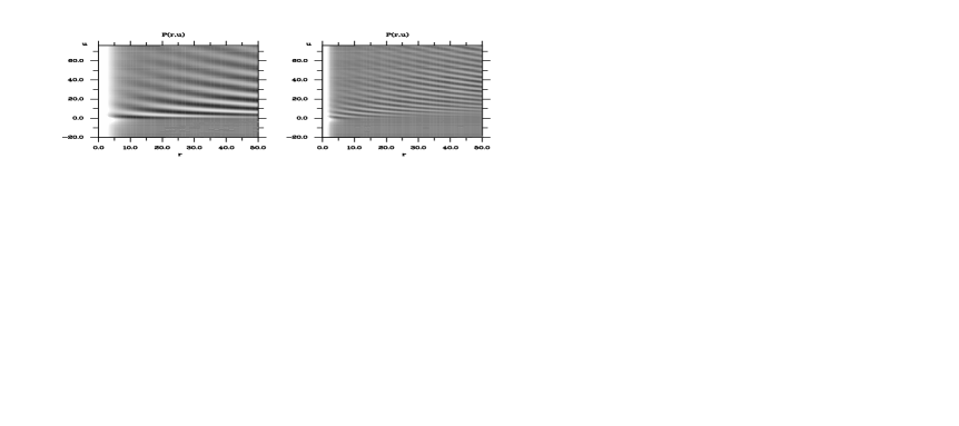
FIG. 8.: The cosmic string variable $P$ is shown as a function of radius and time for $\alpha=0.2$ (left) and $\alpha=1$ (right) (all other parameters have standard values). Note that we use the radial variable $r$ out to $r=50$ here. The ringing can clearly be seen and shows a lower frequency for smaller $\alpha$.

The scenario we are going to investigate in this section is an initially static cosmic string hit by a gravitational wave of Weber–Wheeler type. For this purpose we use the static results with two modifications as initial data. Firstly the static metric function $\nu_{0}$ is multiplied by the exact Weber–Wheeler solution to simulate the gravitational wave pulse. Thus we guarantee that initially the cosmic string is indeed in an equilibrium configuration provided the wave pulse is located sufficiently far away from the origin and its interaction with the string is negligible. Ideally the numerical calculation would start with the incoming wave located at past null infinity. In order to approximate this scenario, we found it was sufficient to use the large negative initial time $u_{0}=-20$. The second modification is to calculate $\gamma$ from the constraint equation (12) to preserve consistency with the Einstein field equations. In Figure 6 the corresponding initial data for $\nu$, $P$ and $X$ are shown for the parameter set $\eta=10^{-3}$, $\alpha=1$, $a=2$ and $b=0.5$. From now on we will refer to these values as “standard parameters” and only specify parameters if they take on non-standard values. Note that $\tau$ vanishes on the initial slice in this case and stays identically zero throughout the evolution. The case of rotating gravitational waves hitting a cosmic string will be analysed in a future publication. The time evolution of the “standard configuration” is shown in Figure 7 where we plot $\nu$, $\mu$, $\gamma$, $P$ and $X$ as functions of $w$ at times $-20$, $-10$, $0$, $2$ and $10$. While the wave pulse is still far away from the origin, its interaction with the cosmic string is negligible (dotted lines). When it reaches the core region, however, it excites the cosmic string and the scalar and vector field start oscillating (dashed curves). After being reflected at the origin, the wave pulse travels along the outgoing characteristics and the metric variables $\nu$, $\mu$ and $\gamma$ quickly settle down into their static configuration which is close to Minkowskian values for $\eta=10^{-3}$. The vector and scalar field of the cosmic string, on the other hand, continue ringing albeit with a different character. Whereas the oscillations of the scalar field $X$ are dominant in the range $r\leq 2$ and have significantly decayed at $u=10$ as shown in the figure, the vector field oscillations propagate to large radii and fall off very slowly (solid curves). This behavior is also illustrated in the right panel of Figure 8 which shows a contour plot of $P$ as a function of $(u,r)$ out to $r=50$. We shall see below, that the oscillations of $P$ will also decay eventually and the cosmic string will asymptotically settle back into its equilibrium configuration.

B Frequency analysis

We will now quantitatively analyse the oscillations of the scalar and vector field of the cosmic string. Since we are working in rescaled coordinates, time and distance are measured in units of $1/\sqrt{\lambda}\eta$ and frequency in its inverse. To avoid complicated notation, however, we will omit the units from now on unless the meaning is unclear. In order to measure frequencies, we Fourier analyse the time evolution of the scalar and vector field for fixed radius $r$. Figure 9 shows $P$ and $X$ for standard parameters as functions of time at $r=1$ together with the corresponding power spectra. The plots for $X$ show a characteristic frequency $f_{X}=0.43$ whereas for $P$ we find a strong peak at $f_{P}=0.16$. The spectrum for $P$, however, also shows a strong mode at $f=0.43$. We have calculated similar power spectra for a large class of parameter sets and discovered this effect on numerous occasions — in addition to a strong peak at the characteristic frequency of $P$ or $X$ there is a second maximum at the characteristic frequency of the other field. In general the characteristic mode of $X$ resulted in stronger peaks at smaller radius, that of $P$ was stronger at larger radii. We attribute this feature to the interaction between the scalar and vector component of the cosmic string. The variation of the relative strength of the oscillations with radius confirms the corresponding observation in Figure 7. The accuracy of the measurements of the frequencies is limited by the resolution of the Fourier spectra which again is limited by the time interval covered in the evolution and, thus, by computation time. For tolerable computation times we get an accuracy $\Delta f\approx 0.01$ which corresponds approximately to one bin in the frequency spectra.

FIG. 9.: Upper panels: The variables $P$ and $X$ at $r=1$ are plotted as functions of $u$ for $\alpha=1$, $\eta=10^{-3}$, $a=2$ and $b=0.5$. Lower panels: The corresponding power spectra. The spectrum for $P$ shows a strong peak at $f=0.16$, that for $X$ at $f=0.43$. The latter component, however, is also clearly present in the spectrum of $P$ which we attribute to the interaction between the fields (see text for details). Note that due to our rescaling of the coordinates, $u$ is measured in units of $1/\sqrt{\lambda}\eta$.

FIG. 10.: The frequencies $f_{P}$ (’+’) and $f_{X}$ (’$\times$’) are plotted as functions of $\alpha$. The curves have been obtained from fitting power laws. For $5\leq\alpha\leq 8$ the expected frequencies for $P$ and $X$ are similar and we found only one maximum in the power spectra. These values are plotted as filled lozenges and have not been included in the regression analysis as their classification is not obvious. The power law for $P$ coincides with the observed values to within measurement accuracy. The frequencies of $X$, however, show a significant, albeit small, deviation from the fitted constant line.

In order to investigate the dependency of the oscillations on $\alpha$, $\eta$, $a$, $b$ and the radial position $r$, we have varied each parameter over at least two orders of magnitude while keeping the other parameters at standard values. We have found the following dependencies:

• The frequencies of both $X$ and $P$ did not show any variations with $\eta$ for $\eta<0.1$. (Note that $\eta$ does, however, appear in the units). For larger values of $\eta$, the non-linear interaction between string and geometry becomes dominant and we did not find a simple relation between frequency maxima and parameters.

• The variation of the parameters $a$ and $b$, the width and amplitude of the Weber–Wheeler pulse, has no measurable effect on the frequencies of $X$ and $P$, but only determined the amplitude of the oscillations. A narrow, strong pulse leads to larger amplitudes.

• For small $r$ the oscillations in $X$ are stronger, whereas those for $P$ dominate at large $r$. The frequency values, however, do not depend on the radius. For radii greater than 10 the oscillations in $X$ had decayed so strongly that we could no longer measure its frequency.

• To first order approximation the frequency of the scalar field, $f_{X}$, is independent of $\alpha$ over the observed range $0.1\leq\alpha\leq 10$. $f_{P}$, however, shows a strong dependence on $\alpha$ which is also illustrated in Figure 8, where we compare contour plots of $P$ obtained for $\alpha=0.2$ and $1$. The frequency is significantly larger for $\alpha=1$.

In Figure 10 we show $f_{P}$ and $f_{X}$ as functions of $\alpha$ together with the power laws obtained from a linear regression of the corresponding double logarithmic data. In the range $5\leq\alpha\leq 8$ (where $\alpha=8$ corresponds to the critical coupling), the expected values of $f_{P}$ and $f_{X}$ become similar and we observed only one maximum in the corresponding power spectra. Therefore a classification with respect to the vector or scalar origin of the frequencies is not obvious. These values (shown by filled lozenges in Figure 10) have not been used in the regression analysis. We obtain power law indices $\sigma_{X}=0.00$ and $\sigma_{P}=0.50$, so that

$$f_{X} \sim {\rm const.}$$ (76)

$$f_{P} \sim \sqrt{\alpha}.$$ (77)

Whereas the fitted curve for $f_{P}$ coincides with the observed values to high accuracy, Figure 10 shows a small but significant deviation of the measured $f_{X}$ from the fitted constant line. Indeed the sizable range over $\alpha$ for which we observe only one frequency indicates significant non-linear interaction similar to the effect of phase locking in non-linear systems of ODEs [12]. If we consider $f_{X}$ and $f_{P}$ to be given by (76) and (77) in terms of the rescaled unphysical coordinates and we transform this back into physical units using $\alpha=e^{2}/\lambda$, we arrive at the following relations for the physical variables

$$f_{X} \sim \sqrt{\lambda}\eta,$$ (78)

$$f_{P} \sim e\eta.$$ (79)

As shown in [5] up to constant factors $\sqrt{\lambda}\eta$ and $e\eta$ are the masses of the scalar and the vector field, $m_{X}$ and $m_{P}$, and we conclude that $X$ and $P$ have characteristic frequencies

$$f_{X} \sim m_{X},$$ (80)

$$f_{P} \sim m_{P}.$$ (81)

Since the frequencies for $X$ and $P$ seem only to depend upon the respective masses we have attempted to confirm these results by considering the oscillations of a cosmic string in two further scenarios. Firstly since the frequencies do not depend upon the Weber–Wheeler pulse we take as initial data the static values for the metric variables but excite the string by adding a Gaussian perturbation to either the $X$ or $P$ static initial values. The evolution is then computed using the fully coupled system. Secondly since the frequencies do not seem to depend upon the strength of the coupling to the gravitational field we have completely decoupled the gravitational field and considered the evolution of a cosmic string in Minkowski spacetime. The initial data is taken to be that for a static string in Minkowski spacetime with a Gaussian perturbation to either the $X$ or $P$ values. The evolution is then computed using the equations for a dynamical string in a Minkowskian background [equations (85) and (86) of paper I]. In both cases we find the same frequencies, to within an amount $\Delta f=0.01$, that we found in the original case of the fully coupled system excited by a Weber–Wheeler pulse. Furthermore the frequencies did not depend on the location or shape of the field perturbation nor upon the choice of $X$ or $P$ as the perturbed field.

C The long term behavior of the dynamic string

FIG. 11.: The upper four plots show the difference between the evolved functions $\nu$, $\mu$, $\gamma$ and $X$ and their corresponding static results. For $P$ a similar 3-dimensional plot is not suitable since it fails to resolve the oscillations of the vector field. Therefore we plot the $\ell_{2}$-norm (dashed line) and the maximum (solid line) of $\Delta P$ as a function of time. $\nu$, $\mu$, $\gamma$ and $X$ quickly settle down in their equilibrium configuration to numerical accuracy. The decay of the oscillations of $P$ takes significantly more time but eventually $P$ also approaches its equilibrium state.

The time evolution shown in Figures 7 and 8 indicate that the oscillations of the cosmic string excited by gravitational waves gradually decay and metric and string settle down into an equilibrium state. We have calculated a very long run ($-20\leq u\leq 410$) to investigate the long term behavior in detail. The unphysically large value of $\eta=0.1$ is chosen for this calculation in order to guarantee a strong interaction between spacetime geometry and the cosmic string. In Figure 11 we show the difference $\Delta f:=f_{\rm evol}-f_{\rm stat}$ between the time-dependent $\nu$, $\mu$, $\gamma$ and $X$ and their corresponding static results obtained for the same parameters. For the vector field $P$ a similar 3-dimensional plot would require an extreme resolution to properly display the oscillations of the vector field (cf. Figure 7). For this reason we proceed differently and calculate the $\ell_{2}$-norm and the maximum of $\Delta P$ for each slice $u={\rm const}$. Both functions are plotted versus time in Figure 11. The incoming wave pulse can clearly be seen as a strong deviation of $\nu$ from the static function. The pulse excites the cosmic string and is reflected at the origin at $u=0$. The metric variables and the scalar field $X$ then quickly reach their equilibrium values. The oscillations in $P$ decay on a significantly longer time scale which is also evident in Figures 7 and 8 and the $\ell_{2}$-norm of $\Delta P$ slowly approaches zero. Significantly longer runs than shown here are prohibited by the required computational time, but the results indicate that $P$ will also eventually reach its equilibrium configuration.

VI Conclusion

In this paper we have described the details of the implicit, fully characteristic, numerical scheme which is used to solve the field equations for a cosmic string coupled to gravity. A feature of the cosmic string equations is that they admit exponentially diverging unphysical solutions. By using a Geroch decomposition it is possible to reformulate the problem in terms of fields which describe the string on an asymptotically flat $2+1$-dimensional metric as well as two auxiliary fields $\nu$ and $\tau$ which describe the gravitational degrees of freedom. We can then introduce a conformally compactified radial coordinate $y$ which allows us to include null infinity as part of the numerical grid. As well as avoiding the need to introduce artificial outgoing boundary conditions at the edge of the grid this approach has the advantage that we can also enforce boundary conditions for the string variables at null infinity which rule out the unphysical solutions. The use of the geometrically defined Geroch variables also improves the long term stability of the code compared to the use of metric variables.

The code has been shown to reproduce the results of two exact vacuum solutions, the Weber–Wheeler solution which describes a pulse of gravitational radiation with just the $+$ polarisation state, and a solution due to Xanthopoulos which describes a gravitational wave with both the $+$ and $\times$ polarisation states. The code has also been shown to reproduce the results of the static cosmic string code in that initial data corresponding to a static solution do not change when evolved in time using the dynamical code. For both the exact vacuum solutions and the static initial data the code shows excellent long term stability. Finally a time dependent convergence analysis demonstrates clear second order convergence of the code.

After demonstrating the reliability of the code we use it to analyse the interaction between an initially static cosmic string and a Weber–Wheeler type pulse of gravitational radiation. We find that the gravitational wave excites the string and causes the string variables $X$ and $P$ to oscillate before the configuration slowly settles back into its equilibrium state. In terms of the unphysical rescaled variables we find that the frequencies of the oscillations are essentially independent of the value of the coupling constant $\eta$ and of the width and amplitude of the Weber–Wheeler pulse. We also find that the frequency of $X$ is independent of $\alpha$ while that of $P$ is proportional to $\sqrt{\alpha}$. When this result is translated back into the physical units we find that the frequency of the scalar field is proportional to the mass of the scalar field and the frequency of the vector field is proportional to the mass of the vector field. This result is confirmed by investigating two further scenarios. Firstly we consider the evolution of static initial data for the string coupled to the gravitational field, but with a Gaussian perturbation to one of the string variables, and secondly we consider the same thing but in a Minkowskian background with the gravitational field decoupled. In both cases we obtain the same relationship between the frequencies and the mass.

Having investigated the interaction between a Weber–Wheeler type pulse of gravitational radiation and the cosmic string, the next obvious step is to consider the interaction between the string and a pulse of gravitational radiation with both polarisation states present. The code will also be a valuable tool in comparing the numerical results with those that one gets from using perturbation theory or the thin string limit to approximate the behavior of a cosmic string coupled to gravity.

- [1] Sjödin K.R.P., Sperhake U. and Vickers J.A., Dynamic Cosmic Strings I, preprint gr-qc/0002096 (2000)
- [2] Jordan P., Ehlers J. and Kundt W., Abh. Wiss. Mainz. Math. Naturwiss., K1, 2 (1960)
- [3] Kompaneets A.S., Sov. Phys. JETP 7, 659 (1958)
- [4] Geroch R., A Method for Generating Solutions of Einstein’s Equations, J. Math. Phys., 12, 918 (1971)
- [5] Shellard E.P.S. and Vilenkin A., Cosmic Strings and other Topological Defects, Cambridge, 1994
- [6] Garfinkle D., General relativistic strings, Phys. Rev. D, 32, 1323 (1985)
- [7] Dubal M.R., d’Inverno R.A. and Clark C.J.S., Combining Cauchy and characteristic codes. II. The interface problem for vacuum cylindrical symmetry, Phys. Rev D, 52, 6868 (1995)
- [8] d’Inverno R.A., Dubal M.R. and Sarkies E.A., Cauchy-characteristic matching for a family of cylindrical solutions possessing both gravitational degrees of freedom, preprint gr-qc/0002057 (2000)
- [9] Press W.H., Teukolsky S.A., Vetterling W.T. and Flannery B.P., Numerical Recepies in C: The art of Scientific Computing, Cambridge, 1992
- [10] Weber J. and Wheeler J.A., Reality of the Cylindrical Gravitational Waves of Einstein and Rosen, Rev. Mod. Phys., 29, 509 (1957)
- [11] Xanthopoulos B.C., Cylindrical waves and cosmic strings of Petrov type D, Phys. Rev. D, 34, 3608 (1986)
- [12] Arnold V.I., Geometrical Methods in the Theory of Ordinary Differential Equations, Springer, 1983