Alberta-Thy-04-00
Quantum Radiation of a Uniformly Accelerated Refractive Body


V. Frolov Β  and D. Singh
e-mail: frolov@phys.ualberta.cae-mail: singh@phys.ualberta.ca
Abstract

We study quantum radiation generated by an accelerated motion of a small body with a refractive index $n$ which differes slightly from 1. To simplify calculations we consider a model with a scalar massless field. We use the perturbation expansion in a small parameter $n-1$ to obtain a correction to the vacuum Hadamard function for a uniformly accelerated motion of the body. We obtain the vacuum expectation for the energy density flux in the wave zone and discuss its properties.

Theoretical Physics Institute, Department of Physics,


University of Alberta, Edmonton, Canada T6G 2J1


PACS number(s): 03.70.+k, 11.10.-z, 42.50.Lc

1 Introduction

Electromagnetic radiation from a uniformly accelerated charge is an example of an β€œeternal problem” of physics. Starting with the work by Born [1] different aspects of this problem have been discussed again and again (see e.g [2, 3] and references therin). In this paper we consider a peculiar quantum analogue of this problem.

Consider a small uncharged body and assume that it has internal degrees of freedom interacting with the electromagnetic field. A polarizable body is a well known example of such a system. Electromagnetic zero-point fluctuations induce dipole moments in the body. If a polarizable body is at rest, corrections to the field connected with this effect after averaging result in the change of the energy of the system. In the presence of two polarizable bodies the energy shift depends on the distance between them and results in the well known Casimir effect (see e.g. [4]–[7]). For an accelerated motion of a polarizable body the net result of the emission of its induced fluctuating dipole moment is quantum radiation, or so called dynamical Casimir effect [10]–[11]. For a non-relativistic motion and relativistic motion in 2 dimensional spacetime this effect is studied quite well, especially in the special case when the polarizability is very high and a surface of the body can be approximated by a reflecting mirror-like boundary [8]–[22]. Much less results have been obtained for the relativistic motion in physical 4 dimensional spacetime. Exception are cases of a uniformely accelerated plane mirror [23] and relativistic expanding spherical mirrors [25]–[26]. See also [27] where quantum radiation from an accelerated spherical body with a mirror boundary was considered. In this paper we study the effect of quantum radiation generated by an accelerated motion of a small polarizable body.

To simplify calculations, we assume that internal degrees of freedom of a body interact not with the electromagnetic field but with a scalar massless field. We assume that a β€œrefractive index” $n$ inside a small ball differs from its vacuum value, 1. To solve the problem, we assume also that $n$ is close to 1 and use the perturbation expansion in a small parameter $n-1$. We consider a simplest accelerated motion when the direction and the value of the acceleration (as measured in the comoving frame) are constant. We calculate a correction to the vacuum Hadamard function created by a uniformly accelerated motion of the body. The main result of the paper is the expression for the quantum average energy density flux at infinity for this problem.

The paper is organized as follows. Section 2 discusses the set up of the problem. We formulate the equation for a massless scalar field in a presence of β€œrefracting” matter and discuss the case when a refractive ball is uniformely accelerated. Section 3 contains the calculation of the perturbed Hadamard function in the presence of the accelerated refractive ball of small size. We also discuss symmetry relations for observables at ${\cal J}^{+}$ connected with the boost invariance of the problem. The expressions for $\langle\hat{\varphi}^{2}\rangle^{\mbox{\tiny{ren}}}$ and $\langle\hat{T}^{\mu}_{\nu}\rangle^{\mbox{\tiny{ren}}}$ in the wave zone are obtained and discussed in SectionΒ 4. SectionΒ 5 contains a discussion of the obtained results.

2 Model

2.1 A β€œrefractive” body in a static spacetime

Our purpose is to study quantum radiation from a an accelerated β€œrefractive” body. We shall use a simplified model by assuming that a body interacts with a quantum massless scalar field $\varphi$.

In order to describe the model let us consider first a static gravitational field described by metric

$$dS^{2}=-A^{2}\,dt^{2}+\gamma_{ij}\,dx^{i}\,dx^{j}\,.$$ (2.1)

Here $A$ and $\gamma_{ij}$ do not depend on $t$; $\xi^{\mu}\,\partial_{\mu}=\partial_{t}$ is a Killing vector, and

$$A^{2}=-\xi^{\mu}\,\xi_{\mu}\,.$$ (2.2)

It is well known (see [28]) that the Maxwell equations in the metric (2.1) are identical to the Maxwell equations in a media with $\varepsilon=\mu=A$. Thus $A^{-1}$ plays the role of the refraction index $n=1/\sqrt{\varepsilon\mu}$. We use this observation to introduce an effective refraction index into the equations for the scalar field.

Consider a new metric $dS_{n}^{2}$ related to (2.1) as follows

$$dS_{n}^{2}=-\,\frac{A^{2}}{n}\,dt^{2}+n\gamma_{ij}\,dx^{i}\,dx^{j}\,,$$ (2.3)

where the effective refraction index $n=n(x^{i})$ does not depend on time $t$. We choose an equation for the scalar field $\varphi$ in the form

$$\Box_{n}\varphi=0\,,$$ (2.4)

where $\Box_{n}$ is the β€œbox”-operator in the metric (2.3). Equation

$$dS_{n}^{2}=0\,,$$ (2.5)

gives characteristics for the equation (2.4). Consider a Killing observer moving with a four-velocity $u^{\mu}=\xi^{\mu}/A$. In the reference frame of this observer, $d\tau=A\,dt$ is a proper time, $dl=\sqrt{\gamma_{ij}\,dx^{i}\,dx^{j}}$ is a proper distance, and equation (2.5) takes the form

$$\frac{dl}{d\tau}=\frac{1}{n}\,.$$ (2.6)

The characteristics of the scalar field equation (2.4) are rays moving with a velocity $c/n$ with respect to a static observer, and hence $n$ really plays the role of the refraction index.

The equation (2.4) can be identically rewritten in the form

$$\Box\varphi=D(n)\,\varphi\,,$$ (2.7)

where

$$D(n)\,\varphi=\frac{n^{2}-1}{A^{2}}\,\partial_{t}^{2}\varphi\,.$$ (2.8)

In the case when $|n-1|\ll 1$, the term $D(n)\varphi$ can be consided as a perturbation111There is an ambiguity in the form of the metric (2.3). One can multiply the metric by any function $f(n)$ which for $n=1$ takes the value 1. This operation would modify the form of the operator $D(n)$. In particular, a term proportional $\nabla n\nabla$ would be generated. For a wave of characteristic frequency $\omega$ it gives a contribution $\sim\omega\Delta n/b$ where $b$ is a size of the body. It can be considered as a perturbation only if it is much smaller than the leading derivative terms of the unperturbed operator which are of the order $\omega^{2}$. For our problem $\omega\sim a$ where $a$ is the acceleration of the body, and $ab\ll 1$. In order to escape problems connected with the applicability of the perturbation approach and to simplify the calculations we choose the special case $f=1$. . It should be emphasized that the form of the operator $D(n)$ implies that equations (2.7)-(2.8) can be easily generalized to the case of a media with dispersion. For a monochromatic wave of frequency $\omega$, $\partial_{t}^{2}\rightarrow-\omega^{2}$, and in order to take into account the dispersion it is sufficient to put $n=n(\omega)$.

In our set-up we assume that $n=1$ everywhere outside some four-dimensional region $\Gamma$ where a refractive body is located, and n=constβ‰ 1𝑛const1n=\,\mbox{const}\ \not=1 inside this region. We assume that a body is static and rigid. Let $B$ be a three-dimensional volume occupied by the body at $t=t_{0}$ and $S=\partial B$ be a surface of the body. Denote by $\Sigma$ a three-dimensional surface formed by Killing trajectories passing through $S$. The region $\Gamma$ is defined as a four-dimensional region located inside $\Sigma$. Thus we have $\Sigma=\partial\Gamma$.

The operator (2.8) in a spacetime with such a body is of the form

$$D(n)=\frac{n^{2}-1}{A^{2}}\,\vartheta(\Gamma)\,\partial_{t}^{2}\,,$$ (2.9)

where $\vartheta$ is the Heavyside step function.

2.2 Uniformly accelerated body

Now we adopt the above scheme to the case of a uniformly accelerated body moving in a flat spacetime. Let $(T,X,Y,Z)$ be standard Cartesian coordinates so that the metric is

$$dS^{2}=-dT^{2}+dX^{2}+dY^{2}+dZ^{2}\,.$$ (2.10)

Denote by $\gamma$ a world line of a uniformly moving observer. If $X$ is the direction of motion and $a$ is the acceleration, $\gamma$ is described by the equation

$$X^{2}-T^{2}=l^{2}\equiv a^{-2}\,.$$ (2.11)

In what follows the length parameter $l$ will play an important role. For this reason it is convenient from the very beginning to introduce dimensional coordinates

$$t=\frac{T}{l}\,,\quad x=\frac{X}{l}\,,\quad y=\frac{Y}{l}\,,\quad z=\frac{Z}{l}\,.$$ (2.12)

Denote

$$x=(1+\xi)\cosh\eta\,,\quad t=(1+\xi)\sinh\eta\,.$$ (2.13)

Then the metric (2.10) takes the Rindler form

$$dS^{2}=l^{2}\left[-(1+\xi)^{2}\,d\eta^{2}+d\xi^{2}+dy^{2}+dz^{2}\right]\,.$$ (2.14)

This metric is valid in the wedge $x>|t|$. The equation (2.11) for $\gamma$ takes the form

$$\xi=0\,,$$ (2.15)

while $l\eta$ is a proper time along $\gamma$.

Surface $\eta=\eta_{0}$ is a plane with a three-dimensional flat metric. It is convenient to introduce spherical coordinates $(\beta,\theta,\phi)$ related to $(\xi,y,z)$ as

$$(\xi,y,z)=\beta n^{i}\,,$$ (2.16)

where

$$n^{i}=(\cos\theta,\sin\theta\cos\phi,\sin\theta\sin\phi)$$ (2.17)

is a unit vector directed from the origin $\xi=y=z=0$ to the point $(\xi,y,z)$.

Consider a small uniformly accelerated body, i.e. with the size much smaller than $l$. Such a body is at rest in the reference frame (2.14). In the general case the surface of the body is described by the equation

$$\beta=\beta_{0}(\theta,\varphi)\,.$$ (2.18)

Relation (2.18) is the equation which defines the surface $\Sigma$, while (2.18) together with $\eta=\eta_{0}$ determines a position of the surface of the body at time $\eta_{0}$. Later we consider a special case when the body is a ball and its surface is a sphere of radius $b$. For this case

$$\beta_{0}=\frac{b}{l}=\mbox{const}\,.$$ (2.19)

3 Quantum Radiation of an Accelerated Refractive Body

3.1 Hadamard functions and stress-energy tensor

To find quantum radiation of an uniformly accelerated body with $|n-1|\ll 1$, we consider the operator $D(n)$ as a perturbation and use perturbation expansion to obtain an answer.

In the absence of the body the field equation is

$$\Box\varphi=0\,.$$ (3.1)

Denote

$$G_{0}^{(1)}(x,x^{\prime})=\langle 0|\hat{\varphi}(x)\,\hat{\varphi}(x^{\prime})+\hat{\varphi}(x^{\prime})\,\hat{\varphi}(x)|0\rangle\,,$$ (3.2)

the Hadamard function for the standard Minkowski vacuum $|0\rangle$. One has

$$G_{0}^{(1)}(x,x^{\prime})=\frac{1}{2\pi^{2}l^{2}}\,\frac{1}{s^{2}(x,x^{\prime})}\,,$$ (3.3)

where

$$s^{2}(x,x^{\prime})=-(t-t^{\prime})^{2}+(x-x^{\prime})^{2}+(y-y^{\prime})^{2}+(z-z^{\prime})^{2}\,,$$ (3.4)

$(t,x,y,z)$ and $(t^{\prime},x^{\prime},y^{\prime},z^{\prime})$ being dimensionless Cartesian coordinates of points $x$ and $x^{\prime}$.

Consider the inhomogeneous equation

$$\Box\varphi=j\,.$$ (3.5)

Its solution is

$$\varphi(x)=\varphi_{0}(x)-l^{4}\int G_{0}^{\mbox{\tiny{ret}}}(x,x^{\prime})\,j(x^{\prime})\,d^{4}x^{\prime}\,.$$ (3.6)

where the retarded Green function $G_{0}^{\mbox{\tiny{ret}}}$ is

$$G_{0}^{\mbox{\tiny{ret}}}(x,x^{\prime})=\frac{1}{2\pi l^{2}}\,\delta(s^{2}(x,x^{\prime}))\,\vartheta(t-t^{\prime})\,.$$ (3.7)

By considering the right-hand side of (2.7) as a perturbation and using (3.6) one gets

$$G^{(1)}(x,x^{\prime})=G_{0}^{(1)}(x,x^{\prime})+G_{\mbox{\tiny{ren}}}^{(1)}(x,x^{\prime})\,,$$ (3.8)

where

$$G_{\mbox{\tiny{ren}}}^{(1)}(x,x^{\prime})=-l^{4}\,\left\{\int_{\Gamma}d^{4}x^{\prime\prime}\left[G_{0}^{\mbox{\tiny{ret}}}(x,x^{\prime\prime})\,D^{\prime\prime}\,G_{0}^{(1)}(x,x^{\prime\prime})\right.\right.$$
$$\hskip 128.0374pt\left.\left.+\,G_{0}^{\mbox{\tiny{ret}}}(x^{\prime},x^{\prime\prime})\,D^{\prime\prime}\,G_{0}^{(1)}(x,x^{\prime\prime})\right]\right\}\,.$$ (3.9)

Notation $D^{\prime\prime}$ indicates that the operator $D$ acts on the argument $x^{\prime\prime}$. We also use notation $G_{\mbox{\tiny{ren}}}^{(1)}$ for $G^{(1)}-G_{0}^{(1)}$. That is this object that is required for the calculation of physically observable quantities obtained by subtracting contribution of zero-point fluctuations in an empty spacetime. The integration in (3.9) is performed over the interior of the world-tube $\Gamma$.

By calculating $G_{\mbox{\tiny{ren}}}^{(1)}(x,x^{\prime})$ we can find $\langle\varphi^{2}\rangle^{\mbox{\tiny{ren}}}$ and $\langle T_{\mu\nu}\rangle^{\mbox{\tiny{ren}}}$ which characterize change in the fluctuations and in the stress-energy tensor generated by the moving body:

$$\langle\varphi^{2}(x)\rangle^{\mbox{\tiny{ren}}}=\frac{1}{2}\,\lim_{x^{\prime}\rightarrow x}G_{\mbox{\tiny{ren}}}^{(1)}(x,x^{\prime})\,,$$ (3.10)
⟨Tμ​ν​(x)⟩ren=limxβ€²β†’xΠμ​ν′​Gren(1)​(x,xβ€²).superscriptdelimited-⟨⟩subscriptπ‘‡πœ‡πœˆπ‘₯rensubscriptβ†’superscriptπ‘₯β€²π‘₯subscriptΞ πœ‡superscriptπœˆβ€²superscriptsubscript𝐺ren1π‘₯superscriptπ‘₯β€²\langle T_{\mu\nu}(x)\rangle^{\mbox{\tiny{ren}}}=\lim_{x^{\prime}\rightarrow x}\Pi_{\mu\nu^{\prime}}\,G_{\mbox{\tiny{ren}}}^{(1)}(x,x^{\prime})\,. (3.11)

Here

$$\Pi_{\mu\nu^{\prime}}=\left(\frac{1}{2}-\xi\right)\nabla_{(\mu}\nabla_{\nu^{\prime})}+\left(\xi-\frac{1}{4}\right)g_{\mu\nu^{\prime}}\,g^{\alpha\beta}\nabla_{\alpha}\nabla_{\beta^{\prime}}-\frac{1}{2}\,\xi\left(\nabla_{(\mu}\nabla_{\nu)}+\nabla_{(\mu^{\prime}}\nabla_{\nu^{\prime})}\right)\,,$$ (3.12)

and $\xi$ is a parameter of non-minimal coupling. For $\xi=0$ one gets the canonical stress-energy tensor, while for $\xi-1/6$ one gets the β€œimproved” one with vanishing trace.

3.2 $\langle\varphi^{2}(x)\rangle^{\mbox{\tiny{ren}}}$ and $\langle T_{\mu\nu}(x)\rangle^{\mbox{\tiny{ren}}}$ on ${\cal J}^{+}$

We shall perform calculations assuming that a point of observation, $x$, is located very far away from the moving body, in the so-called radiation zone. Denote

$$r=\sqrt{x^{2}+y^{2}+z^{2}}\,,\quad u=t-r\,,\quad(x,y,z)=rN^{i}\,,$$
$$N^{i}=(\cos\Theta,\sin\Theta\cos\Phi,\sin\Theta\sin\Phi)\,.$$ (3.13)

The coordinate $u$ is the dimensionless retarded time, and $(r,\Theta,\Phi)$ are spherical coordinates in the inertial reference frame. The wave-zone corresponds to taking the limit $r\rightarrow\infty$ with $u$ and $N^{i}$ fixed.

For calculations it is convenient to make the point splitting in $t$-direction, i.e. to choose $x$ and $x^{\prime}$ (the arguments of $G_{\mbox{\tiny{ren}}}^{(1)}$) so that

$$r=r^{\prime}\,,\quad N^{i}=N^{i^{\prime}}\,.$$ (3.14)

We also put

$$u=u_{0}-\frac{h}{2}\,,\quad u^{\prime}=u_{0}+\frac{h}{2}\,.$$ (3.15)

For such a point splitting, $G_{\mbox{\tiny{ren}}}^{(1)}(x,x^{\prime})$ becomes a function of $r,N^{i},u_{0}$ and $h$:

$$\left.G_{\mbox{\tiny{ren}}}^{(1)}(x,x^{\prime})\right|_{{\mbox{\tiny{point}}\atop\mbox{\tiny{splitted}}}}=G(r,u_{0},N^{i},h)\,.$$ (3.16)

Since $G_{\mbox{\tiny{ren}}}^{(1)}$ is a symmetric function of its coordinates $x$ and $x^{\prime}$, $G$ is an even function of its argument $h$.

To obtain $\langle\varphi^{2}\rangle^{\mbox{\tiny{ren}}}$, (3.10), it is sufficient to put $h=0$ in (3.16). The calculations of the energy density flux are more involved. One obtains

d​Ed​U​d​Ω≑R2β€‹βŸ¨TU​U⟩ren≑r2β€‹βŸ¨Tu​u⟩ren=4​π​r2​limhβ†’0[Ξ u​u​G​(r,u0,Ni,h)],π‘‘πΈπ‘‘π‘ˆπ‘‘Ξ©superscript𝑅2superscriptdelimited-⟨⟩subscriptπ‘‡π‘ˆπ‘ˆrensuperscriptπ‘Ÿ2superscriptdelimited-⟨⟩subscript𝑇𝑒𝑒ren4πœ‹superscriptπ‘Ÿ2subscriptβ†’β„Ž0delimited-[]subscriptΞ π‘’π‘’πΊπ‘Ÿsubscript𝑒0superscriptπ‘π‘–β„Ž\frac{dE}{dUd\Omega}\equiv R^{2}\langle T_{UU}\rangle^{\mbox{\tiny{ren}}}\equiv r^{2}\langle T_{uu}\rangle^{\mbox{\tiny{ren}}}=4\pi r^{2}\lim_{h\rightarrow 0}\left[\Pi_{uu}\,G(r,u_{0},N^{i},h)\right], (3.17)

where

Ξ u​u=18​(1βˆ’4​ξ)β€‹βˆ‚u02βˆ’12β€‹βˆ‚h2.subscriptΠ𝑒𝑒1814πœ‰superscriptsubscriptsubscript𝑒0212superscriptsubscriptβ„Ž2\Pi_{uu}=\frac{1}{8}\left(1-4\xi\right)\partial_{u_{0}}^{2}-\frac{1}{2}\,\partial_{h}^{2}\,. (3.18)

As we shall see, the leading term of $G$ in the wave zone is proportional to $r^{-2}$, so that

$$G(r,u_{0},N^{i},h)=\frac{1}{r^{2}l^{2}}\left[{\cal G}_{1}(u_{0},\Theta)+h^{2}\,{\cal G}_{2}(u_{0},\Theta)+O(h^{4})\right].$$ (3.19)

We include factor $l^{2}$ to restore the correct dimensionality of $G$. Functions ${\cal G}_{1}$ and ${\cal G}_{2}$ are dimensionless. They do not depend on $\Phi$ since the system is invariant with respect to rotation in $(y,z)-$plane. Combining these results, we get

$$\langle\varphi^{2}\rangle^{\mbox{\tiny{ren}}}\sim\frac{{\cal G}_{1}(u_{0},\Theta)}{2r^{2}l^{2}}\,,$$ (3.20)
$$\frac{dE}{dUd\Omega}\sim\frac{1}{l^{2}}\left[\frac{1}{8}\left(1-4\xi\right)\partial_{u_{0}}^{2}{\cal G}_{1}(u_{0},\Theta)-{\cal G}_{2}(u_{0},\Theta)\right].$$ (3.21)

3.3 Boost invariance

An important additional information about $\langle\varphi^{2}\rangle^{\mbox{\tiny{ren}}}$ and the energy flux at ${\cal J}^{+}$ can be obtained by using the symmetry of the problem. The spacetime with a uniformly accelerated body is invariant under boost transformations

$$t\rightarrow\tilde{t}=\gamma(t+vx)\,,$$
$$x\rightarrow\tilde{x}=\gamma(x+vt)\,,$$ (3.22)
$$\tilde{y}=y\,,\quad\tilde{z}=z\,,\quad\gamma=(1-v^{2})^{-1/2}\,.$$

It is easy to determine how this symmetry transformation acts on ${\cal J}^{+}$. To do this, we introduce retarded spherical coordinates $(u,r,\Theta,\Phi)$ and $(\tilde{u},\tilde{r},\tilde{\Theta},\tilde{\Phi})$ for both Minkowski frames $x$ and $\tilde{x}$, and using (3.22), we find the relation between them. In the wave-zone limit, $r\rightarrow\infty$, $(u,\Theta,\Phi)$ – fixed, we have

$$\tilde{r}=\gamma r(1+v\cos\Theta)+\gamma\,\frac{vu\cos\Theta}{1+v\cos\Theta}\,,$$
$$\tilde{u}=\frac{\gamma^{u}}{1+v\cos\Theta}\,,$$ (3.23)
$$\tan\tilde{\Theta}=\frac{\sin\Theta}{\gamma(\cos\Theta+v)}\,,\quad\tilde{\Phi}=\Phi\,.$$

The invariance of $\langle\varphi^{2}\rangle^{\mbox{\tiny{ren}}}$ under the transformation (3.22) requies that

$${\cal G}_{1}(\tilde{u},\tilde{\Theta})=\gamma^{2}(1+v\cos\Theta)^{2}\,{\cal G}_{1}(u,\Theta)\,.$$ (3.24)

The invariance condition (3.24) can be written in the infinitesimal form. For this we put $v=\delta v$ and put the first variation of (3.24) with respect to $\delta v$ at $v=0$ equal to zero. This gives the following relation

$$\left(\frac{\partial\tilde{u}}{\partial v}\right)_{v=0}\partial_{u}{\cal G}_{1}+\left(\frac{\partial\tilde{\Theta}}{\partial v}\right)_{v=0}\partial_{\Theta}{\cal G}_{1}=2\cos\Theta\,{\cal G}_{1}\,.$$ (3.25)

Using (3.23), we get

$$\left(\frac{\partial\tilde{u}}{\partial v}\right)_{v=0}=-u\cos\Theta\,,\quad\left(\frac{\partial\tilde{\Theta}}{\partial v}\right)_{v=0}=-\sin\Theta\,.$$ (3.26)

Hence we have

$$\frac{\partial{\cal G}_{1}}{\partial(\ln u)}+\frac{\partial{\cal G}_{1}}{\partial\ln(\sin{\Theta})}=-2{\cal G}_{1}\,.$$ (3.27)

A general solution of the equation (3.27) can be presented in the form

$${\cal G}_{1}(u,\Theta)=\frac{1}{u^{2}}\,{\cal H}_{1}(\frac{\sin\Theta}{u})\,.$$ (3.28)

In a similar way we get

$${\cal G}_{2}(u,\Theta)=\frac{1}{u^{4}}\,{\cal H}_{2}(\frac{\sin\Theta}{u})\,.$$ (3.29)

4 $\langle\varphi^{2}\rangle^{\mbox{\tiny{ren}}}$ and $\langle T_{\mu\nu}\rangle^{\mbox{\tiny{ren}}}$ in the Wave Zone

4.1 Wave zone approximation

To calculate functions ${\cal G}_{1}$ and ${\cal G}_{2}$, we rewrite (3.9) in a more explicit form. Since integration is performed over the world tube $\Gamma$, it is convenient to write the integral in (3.9) in the Rindler coordinates

$$\int_{\Gamma}d^{4}x^{\prime\prime}\,\ldots=\int d\eta\int d\omega\int_{0}^{\beta_{0}(\theta,\phi)}\beta^{2}\,A\,d\beta\,\ldots\equiv\int d^{4}v\,\ldots\,,$$ (4.1)

where $A=1+\beta\,\cos\theta$, $d\omega=\sin\theta\,d\theta\,d\phi$ and $\beta_{0}$ defines the boundary of the body, see (3.20). In these coordinates we also have

$$D=\frac{(n^{2}-1){\cal D}}{l^{2}}\,,$$ (4.2)
$${\cal D}=A^{-2}\,\vartheta(\beta_{0}(\theta,\phi)-\beta)\,\,\partial_{\eta}^{2}\,.$$ (4.3)

Both Green functions $G_{0}^{\mbox{\tiny{ret}}}$ and $G_{0}^{(1)}$ depend only on the distance $s$ between a point in the wave zone and a point inside or on the boundary of the world tube $\Gamma$. Simple calculations give

$$s^{2}(x,x^{\prime\prime})=-2r\,w-u^{2}+2uA\sinh\eta+1+2\beta n^{1}+\beta^{2}\,,$$ (4.4)

where

$$w=u+\beta\,\mbox{\boldmath$n$}_{\bot}\mbox{\boldmath$N$}_{\bot}-F(\eta)\,A\,,\hskip 14.22636ptF(\eta)=\sinh\eta-N^{1}\cosh\eta\,.$$ (4.5)

Here $(u,r,\Theta,\Phi)$ are retarded spherical coordinates of the point $x$ in the wave zone, and $(\eta,\beta,\theta,\phi)$ are Rindler spherical coordinates of the point $x^{\prime\prime}$ in the tube $\Gamma$. The vectors $n$ and $N$ are defined by equations (2.17) and (3.13), respectively, and $\mbox{\boldmath$n$}_{\bot}=(0,n^{2},n^{3})$, $\mbox{\boldmath$N$}_{\bot}=(0,N^{2},N^{3})$.

An important observation is that the leading, $1/r^{2}$, term of $G_{\mbox{\tiny{ren}}}^{(1)}$ in the wave zone can be obtained by neglecting the terms independent of $r$ in (4.4), that is by using the following approximate expressions

$$s^{2}(x,x^{\prime\prime})\approx-2rw_{-}\,,\quad s^{2}(x^{\prime},x^{\prime\prime})\approx-2rw_{+}\,,$$ (4.6)

where

$$w_{\pm}=w_{0}\pm\frac{h}{2}\,,\quad w_{0}=u_{0}+\beta\,\mbox{\boldmath$n$}_{\bot}\mbox{\boldmath$N$}_{\bot}-F(\eta)\,A\,.$$ (4.7)

Combining all these results and using (3.19), we get

$${\cal G}_{1}(u_{0},\Theta)+h^{2}{\cal G}_{2}(u_{0},\Theta)+\ldots$$
$$\hskip 31.2982pt=\frac{n^{2}-1}{16\pi^{3}}\int d^{4}v\left[\delta(w_{-})\,{\cal D}(\frac{1}{w_{+}})+\delta(w_{+})\,{\cal D}(\frac{1}{w_{-}})\right].$$ (4.8)

We omitted $\vartheta$-function which enters the definition (3.7) of $G_{0}^{\mbox{\tiny{ret}}}$ since a future-directed null cone emitted from a point in the wave zone never crosses the tube $\Gamma$.

4.2 Calculation of integrals

Denote by $I(\eta_{0},h)$ the following integral

$$I(\eta_{0},h)=\int_{-\infty}^{\infty}d\eta\,\delta(w_{-})\,\partial_{\eta}^{2}(\frac{1}{w_{+}})\,.$$ (4.9)

Notice that

$$\partial_{\eta}^{2}(\frac{1}{w_{+}})=\frac{F\,A}{w_{\pm}^{2}}+\frac{2(F^{\prime})^{2}\,A^{2}}{w_{\pm}^{3}}\,,$$ (4.10)

where $(\ )^{\prime}=\partial_{\eta}(\ )$. We use here the following property of the function $F(\eta)$

$$F^{\prime\prime}(\eta)=F(\eta)\,.$$ (4.11)

For Ξ˜β‰ 0Θ0\Theta\not=0, $F(\eta)$ is a monotonically increasing function which changes from $-\infty$ (at $\eta=-\infty$) to $+\infty$ (at $\eta=\infty$). Thus equation $w_{0}(\eta)=c$ has a unique solution for any $c$. We denote by $\eta_{0}$ and $\eta_{\pm}$ the solutions of the following equations

$$w_{0}(\eta_{0})=0\,,\quad w_{0}(\eta_{\pm})=\mp\frac{h}{2}\,.$$ (4.12)

The integral (4.9) can be easily calculated by using the relation

$$\delta(w_{-})=\frac{\delta(\eta_{-})}{F^{\prime}(\eta_{-})\,A}\,.$$ (4.13)

We get

$$I(\eta_{0},h)=\frac{1}{F^{\prime}(\eta_{-})}\left[\frac{1}{h^{2}}F(\eta_{-})+\frac{2}{h^{3}}(F^{\prime}(\eta_{-}))^{2}\,A\right].$$ (4.14)

Now we use the following Taylor expansions

$$\eta_{-}=\eta_{0}+\sum_{n=1}^{\infty}\frac{h^{n}}{n!}\,z_{n}\,,$$ (4.15)
$$w_{0}(\eta_{-})=-A\,\sum_{n=1}^{\infty}\frac{1}{n!}\,F_{0}^{(n)}\,(\eta_{-}-\eta_{0})^{n}\,,$$ (4.16)

where $F_{0}^{(n)}=F^{(n)}(\eta_{0})$. Substituting (4.15) into (4.16) and using (4.11), we solve equation

$$w_{0}(\eta_{-})=\frac{h}{2}$$ (4.17)

to determine $z_{n}$ in terms of $F_{0}$ and $F^{\prime}_{0}$. For calculations we use Maple. The result is

$$z_{1}=-\frac{1}{2AF^{\prime}_{0}}\,,\quad z_{2}=-\frac{F_{0}}{4A^{2}(F^{\prime}_{0})^{3}}\,,\quad z_{3}=-\frac{-3(F_{0})^{2}+(F^{\prime}_{0})^{2}}{8A^{3}(F^{\prime}_{0})^{5}}\,,$$
$$z_{4}=\frac{3F_{0}[-5(F_{0})^{2}+3(F^{\prime}_{0})^{2}]}{16A^{4}(F^{\prime}_{0})^{7}}\,,$$ (4.18)
$$z_{5}=-\frac{3[35(F_{0})^{4}-30(F_{0})^{2}(F^{\prime}_{0})^{2}+3(F^{\prime}_{0})^{4}]}{32A^{5}(F^{\prime}_{0})^{9}}\,.$$

We performed calculations up to the order $h^{5}$ which is required to calculate (4.9) up to the order $h^{2}$.

Next steps of the calculations are the following:

  1. 1.

    Write $F(\eta_{-})$ as

    $$F(\eta_{-})=F_{0}\cosh(\eta_{-}-\eta_{0})+F^{\prime}_{0}\sinh(\eta_{-}-\eta_{0})\,.$$ (4.19)
  2. 2.

    Substitute (4.15) into expression (4.19) and using (4.18) get the expression for $F(\eta_{-})$ in powers of $h$.

  3. 3.

    Use the obtained expansion to calculate $I(\eta_{0},h)$ defined by (4.14).

  4. 4.

    Calculate $J_{0}(\eta_{0},h)=I(\eta_{0},h)+I_{0}(\eta_{0},-h)$ to obtain the expression for

    $$J(\eta_{0},h)=\int_{-\infty}^{\infty}d\eta\left[\delta(w_{-})\,\partial_{\eta}^{2}(\frac{1}{w_{+}})+\delta(w_{+})\,\partial_{\eta}^{2}(\frac{1}{w_{-}})\right].$$ (4.20)

We performed these calculations using Maple. The final result is

$$J(\eta_{0},h)=-\frac{F_{0}\sin^{2}\Theta}{2A^{2}(F^{\prime}_{0})^{5}}\left[1+\frac{h^{2}}{8A^{2}(F^{\prime}_{0})^{4}}\,[(4\cosh^{2}\eta_{0}+3)\cos^{2}\Theta\right.$$
$$\quad\quad\quad\quad\left.-\,8\sinh\eta_{0}\cosh\eta_{0}\cos\Theta-7+4\cosh^{2}\eta_{0}]\right]\,.$$ (4.21)

Thus the right-hand side of (4.8) is

$${n^{2}-1\over 16\pi^{3}}\int d\omega\int_{0}^{\beta_{0}(\theta,\phi)}d\beta\,\beta^{2}\,A^{-1}\,J(\eta_{0},h)\,.$$ (4.22)

In this relation $\eta_{0}$ is a solution of the equation

$$F(\eta_{0})=A^{-1}(u_{0}+\beta\,\mbox{\boldmath$n$}_{\bot}\mbox{\boldmath$N$}_{\bot})\,.$$ (4.23)

Since $\beta\ll 1$, one can solve this equation perturbatively. Let $\tilde{\eta}_{0}$ be a solution of the equation

$$F(\tilde{\eta}_{0})=u_{0}\,,$$ (4.24)

then

$$\eta_{0}-\tilde{\eta}_{0}\approx{\beta\over{F^{\prime}}_{0}}\,(\mbox{\boldmath$n$}_{\bot}\mbox{\boldmath$N$}_{\bot}-u_{0}\cos\theta)\,,$$ (4.25)

where ${F^{\prime}}_{0}={F^{\prime}}(\tilde{\eta}_{0})$. In order to take into account the dependence of $J(\eta_{0},h)$ on $\beta$ it is sufficient to expand $J$ near $\tilde{\eta}_{0}$ and use (4.25). The obtained corrections contain an additional small factor $b/l$, where $b$ is the size of the body. By neglecting this correction and similar corrections in $A$, we get

$${(n^{2}-1)\,V\over 16\pi^{3}l^{3}}\,J_{0}(\tilde{\eta}_{0},h),$$ (4.26)

where $V$ is the volume of the body. By comparison with (4.8) we get

$${\cal G}_{1}(u_{0},\Theta)=-{\cal B}\,\frac{F_{0}\sin^{2}\Theta}{(F^{\prime}_{0})^{5}}\,,$$ (4.27)
$${\cal G}_{2}(u_{0},\Theta)=-{\cal B}\,\frac{F_{0}\sin^{2}\Theta}{8(F^{\prime}_{0})^{9}}\left(4F_{0}^{2}-3\sin^{2}(\Theta)\right)\,,$$ (4.28)

where

$${\cal B}={(n^{2}-1)\,V\over 32\pi^{3}l^{3}}\,.$$ (4.29)

Let us emphasize once again that since we are considering the leading in $b/l$ terms, to calculate $F_{0}$ and $F^{\prime}_{0}$ one must put $b=0$. In particular, $F_{0}=u_{0}$. In order to get $F^{\prime}_{0}$ one must first solve the equation

$$F_{0}\equiv\sinh\eta_{0}-\sin\Theta\cosh\eta_{0}=u_{0}\,,$$ (4.30)

and determine $\eta_{0}=\eta_{0}(u_{0},\cos\Theta)$, ans substitute this value into the definition of $F^{\prime}_{0}$

$$F^{\prime}_{0}\equiv\cosh\eta_{0}-\sin\Theta\sinh\eta_{0}\,.$$ (4.31)

4.3 $\langle\varphi^{2}\rangle^{\mbox{\tiny{ren}}}$ and energy density flux

It is easy to check that ${\cal G}_{1,2}$ obey the symmetry relations (3.28)–(3.29). Really by using relations (4.30) and (4.31) one can rewrite ${\cal G}_{1,2}$ in the form

$${\cal G}_{1}(u,\Theta)=-{\cal B}\,{g_{1}(z)\over u^{2}}\,,\hskip 14.22636pt{\cal G}_{2}(u,\Theta)=-{\cal B}\,{g_{2}(z)\over u^{4}}\,,$$ (4.32)

where $z=\sin(\Theta)/u$ and

$$g_{1}(z)={z^{2}\over(1+z^{2})^{5/2}}\,,\hskip 14.22636ptg_{2}(z)={z^{2}(4-3z^{2})\over 8(1+z^{2})^{9/2}}\,.$$ (4.33)

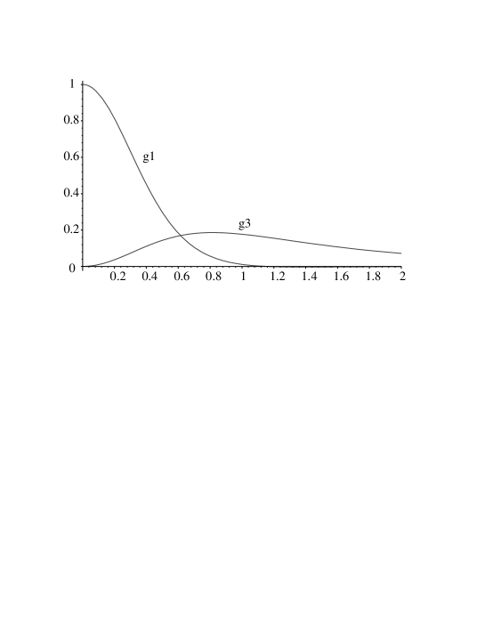
Using equations (3.20) and (3.21), we get

$$\langle\varphi^{2}\rangle^{\mbox{\tiny{ren}}}\sim-\frac{(n^{2}-1)b^{3}ag_{1}(z)}{48\pi^{2}R^{2}U^{2}}\,,$$ (4.34)
$$\frac{dE}{dUd\Omega}=-\frac{(n^{2}-1)b^{3}a}{12\pi^{2}U^{4}}\,(1-5\xi)g_{3}(z)\,.$$ (4.35)

Here

$$g_{3}(z)=\frac{1-3z^{2}/4}{(1+z^{2})^{9/2}}\,.$$ (4.36)

In the previous relations we restored dimensional coordinates $R$ and $U=T-R$, and $z$ which enters these relations is $\sin(\Theta)/(aU)$, where $a$ is the acceleration of the body. Plots of functions $g_{1}$ and $g_{3}$ are shown in FigureΒ 1

Refer to caption

Figure 1: Plots of functions $g_{1}(z)$ ($g1$) and $g_{3}(z)$ ($g3$).

By integrating over angles one gets the total energy density flux

$$\frac{dE}{dU}=-\frac{(n^{2}-1)b^{3}a^{3}}{30\pi U^{2}}\,(1-5\xi)f(aU)\,,$$ (4.37)

where

$$f(u)={1+4u^{2}+5u^{4}+10u^{6}\over(1+u^{2})^{4}}\,.$$ (4.38)

5 Conclusion

In this paper we considered the vacuum polarization effects in the presence of a uniformly accelerated dielectic body. We considered a scalar field model. Under assumption that a size of the body, $b$, is much smaller than the inverse acceleration, $a^{-1}$, we calculated the energy density flux created by the accelerated body at infinity. This flux is given by (4.37), and for the canonical energy (i.e. for $\xi=0$) it is always negative. Its divergence $\sim U^{-2}$ near $U=0$ is connected with the idealization of the problem: it is assumed that the motion remains uniformly accelerated for an infinite interval of time. The boost-invariance property connected with this assumption significantly simplifies calculations. In particular, the quantity $dE/(dUd\Omega)$ giving the anglular distribution of the energy density flux at ${\cal J}^{+}$ at given moment of the retarted time $U$, besides common scale dependence, $U^{-4}$, depends on the function of one variable, $\sin\Theta/aU$.

It would be interesting to repeat calculations for a more realistic case of the electromagnetic field. One can expect that some general features, especially those that are related to the symmetry of the problem, will remain similar to the case of the scalar massless field, while details, such as the angular distribution of the energy flux which might depend on the spin of the field will differ. It should be specially emphasized that the dependence of the electromagnetic field equations on the dielectric and magnetic properties of the media is uniquely fixed, while in the model case of a scalar field there is an ambiguity which we specially fixed to simplify the model.

In our consideration we assumed that a uniformly accelerated refractive body is cold, that is its temperature is zero. One can also consider a case when a body is heated. Especialy interesting is a case when the temperature of he body coincides with the Unruh temperature corresponding to its acceleration. General arguments given in [29, 30] allows one to expect that in this case the quantum radiation vanishes. We hope to return to these problems somewhere else.


Acknowledgments:Β Β  This work was partly supported by the Natural Sciences and Engineering Research Council of Canada. One of the authors (V.F.) is grateful to the Killam Trust for its financial support.


References

  • [1] A. Born, Ann. Physik 30, 1 (1909).
  • [2] T. Fulton and F. Rohlich, Ann. Phys. 9, 499 (1960).
  • [3] V.L. Ginzburg, Soviet Phys. Uspekhi, 98, 569 (1969).
  • [4] H. B. G. Casimir, Proc. K. Ned. akad. Wet. 51, 793 (1948).
  • [5] P. W. Milloni, The Quantum Vacuum, Academic Press, New York, 1994.
  • [6] V. M. Mostepanenko, The Casimir Effect, Cambridge Univ. Press, 1997.
  • [7] β€œThe Casimir Effect: 50 Years Later”, Ed. M. Bordag, World Scientific, Singapore, 1999.
  • [8] G. T. Moore, J. Math. Phys. 11, 2679 (1970).
  • [9] S. A. Fulling, and P. C. W. Davies, Proc. Roy. Soc. A 348, 393 (1976).
  • [10] B. S. DeWitt, Phys. Rep. C 19, 297 (1975).
  • [11] B. D. Birrel and P. C. W. Davies, Quantum Fields in Curved Spacetime, Cambridge Univ. Press, 1982.
  • [12] G. Calucci, J. Phys. A: Math. Gen. 25, 3873 (1992).
  • [13] C. K. Law, Phys. Rev. A 49, 433 (1994).
  • [14] V. V. Dodonov, Phys. Lett. A 207, 126 (1995).
  • [15] O. Meplan and C. Gignoux, Phys. Rev. Lett. 77, 615 (1996).
  • [16] A. Lambrecht, M.-T. Jaekel, and S. Reynaud, Phys. Rev. Lett. 77, 615 (1996).
  • [17] A. Lambrecht, M.-T. Jaekel, and S. Reynaud, Europhys. Lett. 43, 147 (1998).
  • [18] A. Lambrecht, M.-T. Jaekel, and S. Reynaud, Frequency Up-Converted Radiation from a Cavity Moving in Vacuum, E-preprint quant-ph/9805044.
  • [19] R. Colestanian and M. Kardar, Path Integral Approach to the Dynamical Casimir Effect with Fluctuating Boundaries, E-preprint quant-ph/9802017.
  • [20] G. Barton and C. Eberlein, Ann. Phys. (N.Y.) 227, 222 (1993).
  • [21] G. Barton, Ann. Phys. (N.Y.) 245, 361 (1996).
  • [22] G. Barton and C. A. North, Ann. Phys. (N.Y.) 252, 222 (1996).
  • [23] P. Candelas and S. Deutsch, Proc. R. Soc. A 354, 79 (1977).
  • [24] V. P. Frolov and E. M. Serebriany, Journ. Phys A 12, 2415 (1979).
  • [25] V. P. Frolov and E. M. Serebriany, Journ. Phys A 13, 3205 (1980).
  • [26] V. Frolov and D. Singh. Class. Quantum Grav. 16, 3693 (1999).
  • [27] V.Ye. Kur’yan and V.P. Frolov, In:The Physical Effects in the Gravitational Field of Black Holes, Proceedings of the P.N. Lebedev Physical Institute, v. 169 (Ed. M.A. Markov), 219 (1987).
  • [28] L. D. Landau and E. M. Lifshitz, The classical theory of fields, Oxford, Pergamon Press; Reading, Mass., Addison-Wesley Pub. Co., 1962.
  • [29] D.W. Sciama, P. Candelas, D. Deutsch, Adv.Phys. 30, 327 (1981).
  • [30] P. Candelas, D.W. Sciama, Phys.Rev. D27 1715, (1983).