Unexpectedly large surface gravities for acoustic horizons?

Abstract

Acoustic black holes are fluid dynamic analogs of general relativistic black holes, wherein the behaviour of sound waves in a moving fluid acts as an analog for scalar fields propagating in a gravitational background. Acoustic horizons, which are intimately related to regions where the speed of the fluid flow exceeds the local speed of sound, possess many of the properties more normally associated with the event horizons of general relativity, up to and including Hawking radiation. Acoustic black holes have received much attention because it would seem to be much easier to experimentally create an acoustic horizon than to create an event horizon. In this note we wish to point out some potential difficulties (and opportunities) in actually setting up an experiment that possesses an acoustic horizon. We show that in zero-viscosity, stationary fluid flow with generic boundary conditions, the creation of an acoustic horizon is accompanied by a formally infinite “surface gravity”, and a formally infinite Hawking flux. Only by applying a suitable non-constant external body force, and for very specific boundary conditions on the flow, can these quantities be kept finite. This problem is ameliorated in more realistic models of the fluid. For instance, adding viscosity always makes the Hawking flux finite (and typically large), but doing so greatly complicates the behaviour of the acoustic radiation — viscosity is tantamount to explicitly breaking “acoustic Lorentz invariance”. Thus, this issue represents both a difficulty and an opportunity — acoustic horizons may be somewhat more difficult to form than naively envisaged, but if formed, they may be much easier to detect than one would at first suppose.

 

E-mail: liberati@sissa.it

E-mail: sebastiano.sonego@uniud.it

E-mail: visser@kiwi.wustl.edu

Homepage: http://www.sissa.it/~liberati

Homepage: http://www.physics.wustl.edu/~visser

Archive: gr-qc/0003105

 

1 Introduction

Acoustic black holes are very useful toy models that share many of the fundamental properties of the black holes of general relativity, while having a very clear and clean physical interpretation in terms of ordinary non-relativistic fluid mechanics [1, 2, 3, 4, 5, 6, 7, 8]. The fundamental idea is that sound waves propagating in a flowing fluid share many of the formal properties of massless scalar fields propagating in a general-relativistic curved spacetime. Indeed, the propagation of acoustic disturbances in a flowing fluid is described by a spacetime metric with Lorentzian signature, the “acoustic metric”, which is built up algebraically out of the density, velocity, and local speed of sound of the fluid. When the flow is such that there is a surface where the normal component of the fluid velocity equals the speed of sound, the acoustic metric possesses the properties that characterize a black hole spacetime in general relativity, and such a surface is therefore called “acoustic horizon”.

As emphasized in [6, 7], acoustic black holes share all the kinematic aspects of relativistic black holes, but do not share in the dynamic aspects. In particular, acoustic black holes exhibit Hawking radiation from the acoustic horizon, giving rise to a quasi-thermal bath of phonons with temperature proportional to the “surface gravity” (related to the physical acceleration of the fluid as it crosses the acoustic horizon), but they exhibit no simple analog of the Bekenstein–Hawking entropy (since that is a dynamical effect intimately related to the existence of the Einstein equations in general relativity).

One of the reasons why acoustic black holes are so popular is that it seems that the prospects for experimentally building an acoustic horizon are much better than for a general relativistic event horizon. An early estimate can be found in [1], and related comments are to be found in [6, 7]. Additionally, an impressive body of work is due to Volovik and collaborators, who have extensively studied the experimental prospects for building such a system using superfluids such as ³He and ⁴He [9, 10, 11, 12, 13, 14, 15, 16, 17, 18]. These particular implementations of acoustic geometry make extensive use of the two-fluid model of superfluidity, whereas in this paper we will be focussing on a conceptually simpler one-fluid model; accordingly, some important technical details will differ. For yet another physical implementation of acoustic geometries, Garay et al. have investigated the technical requirements for implementing an acoustic horizon in Bose–Einstein condensates [19], and some of the perils and pitfalls accompanying acoustic black holes have been discussed in Jacobson’s mini-survey [20].

Another attractive feature of acoustic black holes is that they seem to be generic, and that they illustrate an important aspect of Lorentz invariance. For instance, it is now known, due to the work of Nielsen and collaborators [21, 22, 23], that in renormalizable non-Lorentz-invariant quantum field theories, Lorentz invariance is often an infrared fixed point of the renormalization group equations. Thus, Lorentz invariance can emerge as a symmetry in the low-energy limit even if the underlying physics is not explicitly Lorentz invariant. Similarly, in acoustic black holes the underlying physics is explicitly classical and Newtonian, but the physics of sound propagation nevertheless exhibits a low-frequency approximate Lorentzian symmetry [6, 7].

In this note we wish to point out a potential difficulty and an opportunity — we shall demonstrate that there is a regularity issue that becomes serious at the acoustic horizon. Either the Hawking temperature is formally infinite (which is the generic situation), or there must be a very precise relationship between an external body force that must be applied to the fluid as it crosses the acoustic horizon and the extrinsic geometry of the latter. If this condition is not satisfied the “surface gravity” formally diverges, as well as the corresponding Hawking temperature. Similarly, the acceleration and density gradient of the fluid at the horizon are formally infinite. For a specified external force, such divergences are generic, in the sense that they are present for almost all flows, except — in some cases — for a set of measure zero that satisfy very special boundary conditions. However, in the case of a constant force (including zero force), which is perhaps the most interesting one from the point of view of laboratory simulations, no boundary conditions exist that correspond to an everywhere regular flow.

On the one hand this result suggests that detecting the acoustic Hawking effect should be very easy; on the other hand it implies that the naive analysis (which demands that both the vorticity and the viscosity be zero) should in some way be modified near the acoustic horizon, at least when the external forces are such that a formal divergence will certainly occur. For instance, adding finite viscosity to the fluid equations is sufficient in order to regulate the surface gravity and Hawking temperature for any choice of external force — though finite they can remain large, and can be much larger than naively expected.

2 Basic equations and assumptions

The acoustic model of Lorentzian geometry arises from the description of the deceptively simple phenomenon of the propagation of sound waves in a flowing fluid. Let us therefore recall the fundamental equations of fluid dynamics, i.e., the equation of continuity

$${\partial\rho\over\partial t}+\vec{\nabla}\cdot\left(\rho\,{\vec{v}\,}\right)=0,$$ (2.1)

and the Euler equation

$$\rho\;\vec{a}=\vec{f},$$ (2.2)

where

$$\vec{a}={\partial{\vec{v}\,}\over\partial t}+({\vec{v}\,}\cdot\vec{\nabla}){\vec{v}\,}$$ (2.3)

is the fluid acceleration, and $\vec{f}$ stands for the force density — the sum of all forces acting on the fluid per unit volume. We shall assume that the external forces present are all gradient-derived (possibly time-dependent) body forces, which for simplicity we lump together in a generic term $-\rho\,\vec{\nabla}\Phi$. In addition to the external forces, $\vec{f}$ contains a contribution from the pressure of the fluid and, possibly, a term coming from viscosity. Thus, equation (2.2) takes the Navier-Stokes form

$$\rho\left({\partial{\vec{v}\,}\over\partial t}+({\vec{v}\,}\cdot\vec{\nabla}){\vec{v}\,}\right)=-\vec{\nabla}p-\rho\;\vec{\nabla}\Phi+{{\vec{f}_{\mathrm{viscous}}}},$$ (2.4)

where

$${{\vec{f}_{\mathrm{viscous}}}}=\eta\nabla^{2}{\vec{v}\,}+\left(\zeta+{1\over 3}\,\eta\right)\vec{\nabla}(\vec{\nabla}\cdot{\vec{v}\,})$$ (2.5)

represents the force due to viscous processes, the coefficients $\eta$ and $\zeta$ giving the dynamic and bulk viscosity, respectively [24, 25].

In deriving the acoustic geometry, one usually makes a number of technical assumptions.

• The first assumption is that the fluid has a barotropic equation of state, that is, the density $\rho$ is a function only of the pressure $p$, so

  $$\rho=\rho(p).$$ (2.6)

  This guarantees that (2.1) and (2.4) are a closed set of equations. We shall consequentely define the speed of sound as

  $$c^{2}={{\mathrm{d}}p\over{\mathrm{d}}\rho}.$$ (2.7)

• The second assumption is that we have a vorticity-free flow, i.e., that $\vec{\nabla}\times{\vec{v}\,}=\vec{0}$. This condition is generally fulfilled by the superfluid components of physical superfluids.

• A third assumption, often made in the existing literature on acoustic geometries, is a viscosity-free flow. Although this is quite a realistic condition for superfluids we shall see that the presence or absence of viscosity can mark a sharp difference in the behaviour of the phonon radiation from acoustic horizons.

These assumptions are sufficient conditions under which an acoustic metric can be written. However, since the following analysis is independent of the introduction of the acoustic geometry (although motivated by it, of course), we shall try to be as general as possible, making use of them only progressively, as they are needed in order to have an analytically tractable system.

3 Regularity conditions at ergo-surfaces

Let us start by establishing a useful mathematical identity. If we write ${\vec{v}\,}=v{\vec{n}\,}$, where ${\vec{n}\,}$ is a unit vector and $v\geq 0$, then

$$\vec{\nabla}\cdot{\vec{v}\,}={{\mathrm{d}}v\over{\mathrm{d}}n}+v\;K,$$ (3.1)

where ${\mathrm{d}}/{\mathrm{d}}n={\vec{n}\,}\cdot\vec{\nabla}$ and $K=\vec{\nabla}\cdot{\vec{n}\,}$. If the Frobenius condition is satisfied, then there exist surfaces orthogonal to the fluid flow. In this situation, $K$ admits a geometrical interpretation as the trace of the extrinsic curvature of these surfaces. It must be noted that, although zero vorticity is a sufficient condition for this to happen, it is not necessary.

We now focus our attention on the component of the fluid acceleration along the flow, $a_{n}=\vec{a}\cdot{\vec{n}\,}$. This can be obtained straightforwardly by projecting the Navier-Stokes equation (2.4) along ${\vec{n}\,}$:

$$\rho\,a_{n}=-c^{2}\,{{\mathrm{d}}\rho\over{\mathrm{d}}n}-\rho\,{{\mathrm{d}}\Phi\over{\mathrm{d}}n}+{\vec{n}\,}\cdot{{\vec{f}_{\mathrm{viscous}}}},$$ (3.2)

where we have used the barotropic condition.

Next, we rewrite the continuity equation as

$${\partial\rho\over\partial t}+v\,{{\mathrm{d}}\rho\over{\mathrm{d}}n}+\rho\left({{\mathrm{d}}v\over{\mathrm{d}}n}+vK\right)=0,$$ (3.3)

where the identity (3.1) has been used. We can express ${\mathrm{d}}v/{\mathrm{d}}n$ in terms of $a_{n}$ noticing that, by the definition (2.3) of $\vec{a}$,

$$a_{n}={\partial v\over\partial t}+v\,{{\mathrm{d}}v\over{\mathrm{d}}n}.$$ (3.4)

Thus, equation (3.3) can be rewritten as

$$\rho\;a_{n}=-v^{2}\,{{\mathrm{d}}\rho\over{\mathrm{d}}n}-\rho v^{2}K+\rho\,{\partial v\over\partial t}-v\,{\partial\rho\over\partial t}\;.$$ (3.5)

Equations (3.2) and (3.5) can be solved for both $a_{n}$ and ${\mathrm{d}}\rho/{\mathrm{d}}n$, obtaining:

$$a_{n}={1\over c^{2}-v^{2}}\left[v^{2}\left({{\mathrm{d}}\Phi\over{\mathrm{d}}n}-c^{2}K-{1\over\rho}\,{\vec{n}\,}\cdot{{\vec{f}_{\mathrm{viscous}}}}\right)+c^{2}\left({\partial v\over\partial t}-{v\over\rho}\,{\partial\rho\over\partial t}\right)\right];$$ (3.6)

$${{\mathrm{d}}\rho\over{\mathrm{d}}n}={1\over c^{2}-v^{2}}\left[-\rho\left({{\mathrm{d}}\Phi\over{\mathrm{d}}n}-v^{2}K-{1\over\rho}\,{\vec{n}\,}\cdot{{\vec{f}_{\mathrm{viscous}}}}\right)-\rho\,{\partial v\over\partial t}+v\,{\partial\rho\over\partial t}\right].$$ (3.7)

In general we see that there is risk of a divergence in the acceleration and the density gradient as $v\to c$, which indicates that the ergo-surfaces (the boundaries of ergo-regions) must be treated with some delicacy. The fact that gradients diverge in this limit is the key observation of this paper; we shall demonstrate that this has numerous repercussions throughout the physics of acoustic black holes.

Since $v^{2}=c^{2}$ at the ergo-surface it is evident that the acceleration and the density gradient both diverge, unless the condition

$${{\mathrm{d}}\Phi\over{\mathrm{d}}n}-c^{2}K-{1\over\rho}\,{\vec{n}\,}\cdot{{\vec{f}_{\mathrm{viscous}}}}+{\partial v\over\partial t}-{c\over\rho}\,{\partial\rho\over\partial t}=0$$ (3.8)

is satisfied on the ergo-surface. Equation (3.8) is therefore a relationship that must be satisfied in order to have a physically acceptable model. Of course, it is only a necessary condition, because $a_{n}$ and ${\mathrm{d}}\rho/{\mathrm{d}}n$ may diverge at the ergo-surface even when (3.8) is fulfilled, if the quantities in square brackets in the right hand sides of (3.6) and (3.7) tend to zero slower than $c^{2}-v^{2}$ as one approaches the ergo-surface.

For a stationary, non-viscous flow, (3.8) reduces to

$${{\mathrm{d}}\Phi\over{\mathrm{d}}n}=c^{2}K,$$ (3.9)

where again $d\Phi/{\mathrm{d}}n$, $c$, and $K$ are evaluated at a generic point on the ergo-surface. Thus, in this case it seems that a special fine-tuning of the external forces is needed in order to keep the acceleration and density gradient finite at the ergo-surface. If the condition (3.9) is not fulfilled but still ${{\vec{f}_{\mathrm{viscous}}}}=\vec{0}$, the flow cannot be stationary. Near the ergo-surface, an instability will make the time derivatives in (3.8) different from zero, so that they could compensate the mismatch between the two sides of (3.9). More realistically, we shall see later that for a given potential, either no horizon forms, or the flow tries to assume a configuration in which (3.9) is automatically satisfied.

4 Regularity conditions at horizons

If we now look at the “surface gravity” of an acoustic black hole it is most convenient to first restrict attention to a stationary flow. Defining a notion of surface gravity for non-stationary flows is easier in fluid mechanics than in general relativity, but is still sufficiently messy to encourage us to make this simplifying assumption [6]. For additional technical simplicity we shall further assume that at the acoustic horizon (the boundary of the trapped region) the fluid flow is normal to the horizon. Under these circumstances the technical distinction between an ergo-surface and an acoustic horizon vanishes and we can simply define an acoustic horizon by the condition $v=c$. (In complete generality you would have to define an [apparent] acoustic horizon as a surface for which the inward normal component of the fluid velocity is everywhere equal to the speed of sound [6]; this adds extra layers of technical complication to the discussion which in the present context we have not found to be useful.) Then it can be shown that the surface gravity $g_{H}$ has two terms [6, 7], one coming from acceleration of the fluid, the other coming from variations in the local speed of sound. More precisely, $g_{H}$ is given by the value attained by the quantity

$$g={1\over 2}\left.{{\mathrm{d}}(c^{2}-v^{2})\over{\mathrm{d}}n}\right.={1\over 2}\left.{{\mathrm{d}}c^{2}\over{\mathrm{d}}n}\right.-a_{n}$$ (4.1)

at the acoustic horizon. (And note that $g$ is defined throughout all space.)

Now we write, using equations (3.3) and (3.4),

$${{\mathrm{d}}c^{2}\over{\mathrm{d}}n} = {{\mathrm{d}}c^{2}\over{\mathrm{d}}\rho}\;{{\mathrm{d}}\rho\over{\mathrm{d}}n}$$ (4.2)

$$= -{{\mathrm{d}}^{2}p\over{\mathrm{d}}\rho^{2}}\left[\rho\left(K+{1\over v}{{\mathrm{d}}v\over{\mathrm{d}}n}\right)+{1\over v}\,{\partial\rho\over\partial t}\right]$$

$$= -{{\mathrm{d}}^{2}p\over{\mathrm{d}}\rho^{2}}\left[\rho\left(K+{a_{n}\over v^{2}}-{1\over v^{2}}\,{\partial\rho\over\partial t}\right)+{1\over v}\,{\partial\rho\over\partial t}\right],$$

so we find, using (3.6):

$$g = {1\over c^{2}-v^{2}}\left[\left(c^{2}+{\rho\over 2}\,{{\mathrm{d}}^{2}p\over{\mathrm{d}}\rho^{2}}\right)\left(Kv^{2}-{\partial v\over\partial t}+{v\over\rho}\,{\partial\rho\over\partial t}\right)\right.$$ (4.3)

$$\left.-\left(v^{2}+{\rho\over 2}\,{{\mathrm{d}}^{2}p\over{\mathrm{d}}\rho^{2}}\right)\left({{\mathrm{d}}\Phi\over{\mathrm{d}}n}-{1\over\rho}\,{\vec{n}\,}\cdot{{\vec{f}_{\mathrm{viscous}}}}\right)\right].$$

Under the present assumptions, time derivatives vanish and $v^{2}=c^{2}$ at the horizon, so it is now evident that the surface gravity (as well as the acceleration and the density gradient) diverges unless the condition

$$\left.{{\mathrm{d}}\Phi\over{\mathrm{d}}n}\right|_{H}-c_{H}^{2}K_{H}-{1\over\rho_{H}}\,{\vec{n}\,}_{H}\cdot({{\vec{f}_{\mathrm{viscous}}}})_{H}=0$$ (4.4)

is satisfied. For a non-viscous flow (4.4) again reduces to (3.9), and the same considerations made about the acceleration and density gradient apply.

Now all this discussion is predicated on the fact that acoustic horizons actually form, and would be useless in the case that some obstruction could be proven to prevent the fluid from reaching the speed of sound. In order to deal with this possibility we shall now check that at least in some specific examples it is possible to form acoustic horizons under the current hypotheses. For analyzing these specific cases it is useful to first consider generic stationary, spherically symmetric flow.

5 Spherically symmetric stationary flow

For simplicity, we now deal with the case of a spherically symmetric stationary flow in $d$ space dimensions. Spherical symmetry guarantees that the fluid flowlines are always perpendicular to the acoustic horizon, and so we can ignore the subtleties attendant on the distinction between horizons and ergospheres [6]. Additionally, for the time being we shall assume the absence of viscosity, ${{\vec{f}_{\mathrm{viscous}}}}=\vec{0}$.

For a spherically symmetric steady inflow, ${\vec{n}\,}$ is minus the radial unit vector. Then ${\mathrm{d}}{\vec{n}\,}/{\mathrm{d}}n={\vec{0}}$; also

$${{\mathrm{d}}\over{\mathrm{d}}n}=-{{\mathrm{d}}\over{\mathrm{d}}r},$$ (5.1)

and

$$K=-{d-1\over r}.$$ (5.2)

From equation (2.3) it follows that $\vec{a}$ has only the radial component, which coincides with $-a_{n}$ and is

$$a=-v^{2}\;{c^{2}{(d-1)/r}-{{\mathrm{d}}\Phi/{\mathrm{d}}r}\over c^{2}-v^{2}}.$$ (5.3)

This result could also be obtained directly, without the general treatment of section 3. For a steady flow the continuity equation implies

$$\rho\;v\;r^{d-1}=J=\mbox{const}.$$ (5.4)

Taking the logarithmic derivative of the above equation one gets

$${{\mathrm{d}}\rho\over{\mathrm{d}}r}=-\rho{(d-1)\over r}-{\rho\over v}\;{{\mathrm{d}}v\over{\mathrm{d}}r}.$$ (5.5)

On the other hand the Euler equation (2.4) takes in this case the form

$$\rho\;v\;{{\mathrm{d}}v\over{\mathrm{d}}r}=-c^{2}\;{{\mathrm{d}}\rho\over{\mathrm{d}}r}-\rho{{\mathrm{d}}\Phi\over{\mathrm{d}}r},$$ (5.6)

where we have used the barotropic condition. Equations (5.5) and (5.6) can be combined to give the useful result

$$v\;{{\mathrm{d}}v\over{\mathrm{d}}r}=c^{2}\left({(d-1)\over r}+{1\over v}\;{{\mathrm{d}}v\over{\mathrm{d}}r}\right)-{{\mathrm{d}}\Phi\over{\mathrm{d}}r},$$ (5.7)

which allows one to easily compute the acceleration $a=v\,{\mathrm{d}}v/{\mathrm{d}}r$ of the fluid for this specific case, recovering equation (5.3), and to obtain a differential equation for the velocity profile $v(r)$:

$${{\mathrm{d}}v\over{\mathrm{d}}r}=-v\;{c^{2}{(d-1)/r}-({\mathrm{d}}\Phi/{\mathrm{d}}r)\over c^{2}-v^{2}}.$$ (5.8)

When it comes to calculating $g$, the same analysis as previously developed now yields

$$g={1\over c^{2}-v^{2}}\left[\left(v^{2}+{\rho\over 2}\,{{\mathrm{d}}^{2}p\over{\mathrm{d}}\rho^{2}}\right){{\mathrm{d}}\Phi\over{\mathrm{d}}r}-\left(c^{2}+{\rho\over 2}\,{{\mathrm{d}}^{2}p\over{\mathrm{d}}\rho^{2}}\right){v^{2}(d-1)\over r}\right].$$ (5.9)

So the acceleration at the acoustic horizon, whose location $r_{H}$ is the solution of the equation $v(r_{H})^{2}=c(r_{H})^{2}$, formally goes to infinity unless the external body force satisfies the condition

$$\left.{{\mathrm{d}}\Phi\over{\mathrm{d}}r}\right|_{H}-c^{2}_{H}\;{(d-1)\over r_{H}}=0.$$ (5.10)

Any further analysis requires one to integrate the differential equation (5.8). However, this can be done only assigning an equation of state $p=p(\rho)$, and integrating simultaneously equation (5.5) in order to get the dependence of $c$ on $r$. We consider such a specific model in the next section.

6 Constant speed of sound

In order to get further insight, let us consider the simple case of a fluid with a constant speed of sound,

$${{\mathrm{d}}^{2}p\over{\mathrm{d}}\rho^{2}}=0.$$ (6.1)

It is easy to see that in this case, the condition (5.10) is also sufficient in order to keep the physical quantities finite on the horizon. Consider equation (5.8) and apply the Bernoulli–de L’Hospital rule in order to evaluate $({\mathrm{d}}v/{\mathrm{d}}r)_{H}$. One gets

$$\left({{\mathrm{d}}v\over{\mathrm{d}}r}\right)^{2}_{H}=-{1\over 2}\left(\left.{{\mathrm{d}}^{2}\Phi\over{\mathrm{d}}r^{2}}\right|_{H}+{c^{2}(d-1)\over r_{H}^{2}}\right),$$ (6.2)

so $({\mathrm{d}}v/{\mathrm{d}}r)_{H}$ has a finite value. As a corollary of (6.2), we see that at the horizon one must have

$$\left.{{\mathrm{d}}^{2}\Phi\over{\mathrm{d}}r^{2}}\right|_{H}\leq-{c^{2}(d-1)\over r_{H}^{2}};$$ (6.3)

so, in particular, no potential with a non-negative second derivative can lead to a horizon on which ${\mathrm{d}}v/{\mathrm{d}}r$ is finite.

With the assumption (6.1), the differential equation (5.8) for the velocity profile can be easily integrated. Its general solution is

$$\frac{1}{2}\left[c^{2}\;\ln\left(\frac{v^{2}}{v^{2}_{0}}\right)-v^{2}+v^{2}_{0}\right]=-c^{2}\;\left(d-1\right)\;\ln{\left(\frac{r}{r_{0}}\right)}+\Phi(r)-\Phi(r_{0}),$$ (6.4)

where $r_{0}$ is arbitrary and $v_{0}$ is the speed of the fluid at $r_{0}$. In order to study the general properties of $v(r)$, it is convenient to rewrite equation (6.4) in the form

$$r^{2(d-1)}{\rm e}^{-2\Phi(r)/c^{2}}W^{-1}\left(-v^{2}/c^{2}\right)=r_{0}^{2(d-1)}{\rm e}^{-2\Phi(r_{0})/c^{2}}W^{-1}\left(-v_{0}^{2}/c^{2}\right),$$ (6.5)

where $W^{-1}$ is the inverse of the Lambert function [26], defined as $W^{-1}(x)=x\;{\rm e}^{x}$. Given $r_{0}$ and $v_{0}$, equation (6.5) implies that the solution $v(r)$ has two branches — a subsonic and a supersonic one. This follows immediately from the trivial fact that, since $W^{-1}(-v_{0}^{2}/c^{2})$ is negative, also $W^{-1}(-v^{2}/c^{2})$ is negative; then, from the plot in figure 1 we see that there are two possible values for $v^{2}$, one smaller and the other greater than $c^{2}$.

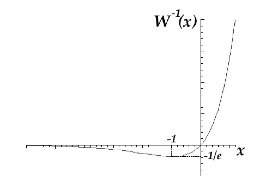
Figure 1: The inverse of the Lambert function: $W^{-1}(x)=x\,{\rm e}^{x}$.

We end this section with some remarks that are crucial for a correct interpretation of the regularity condition (5.10). On rewriting (6.4) or (6.5) as

$$F(r,v;r_{0},v_{0})=0,$$ (6.6)

we can represent the location $r_{H}$ of the horizon, for a given potential $\Phi$ and given boundary data $(r_{0},v_{0})$, as the solution of the equation

$$F(r_{H},c;r_{0},v_{0})=0.$$ (6.7)

On the other hand, differentiating (6.6) and comparing with (5.8) we can rewrite the regularity condition (5.10) as

$${\partial F\over\partial r}(r_{H},c;r_{0},v_{0})=0.$$ (6.8)

It is clear that, if we impose the boundary data $(r_{0},v_{0})$, then (6.8) expresses a fine-tuning condition on $\Phi$ in order to have ${\mathrm{d}}v/{\mathrm{d}}r$ finite at the horizon. However, we can reverse the argument and consider the more realistic case in which one looks for a physically acceptable flow compatible which an assigned $\Phi$, without trying to force the boundary condition $v(r_{0})=v_{0}$ on the velocity profile. In this case, equations (6.7) and (6.8), when solved simultaneously, give the location of the horizon, $r_{H}$, and the value $v_{0}$ of the fluid speed at $r_{0}$. Thus, requiring regularity of the flow for a given potential amounts to solving an eigenvalue problem, while if one insists on assigning a boundary condition for the speed, a careful fine tuning of $\Phi$ is needed in order to avoid infinite gradients. We stress, however, that although from a strictly mathematical point of view both types of problems can be considered, it is the first one that is relevant in practice.

7 Examples

We now consider some specific choices, both of $\Phi(r)$ and of $v(r)$, in order to illustrate the general situation.

7.1 Constant body force

Let us begin with a constant body force, with the linear potential

$$\Phi(r)=\kappa\;r,$$ (7.1)

where $\kappa$ is a constant. Equation (6.4) becomes, in this case,

$$\frac{1}{2}\left[c^{2}\;\ln\left(\frac{v^{2}}{v^{2}_{0}}\right)-v^{2}+v^{2}_{0}\right]=-c^{2}\;\left(d-1\right)\;\ln{\left(\frac{r}{r_{0}}\right)}+\kappa(r-r_{0}),$$ (7.2)

and equation (6.5) can be rewritten completely in terms of inverse Lambert functions:

$$W^{-1}\left(-{\kappa r\over c^{2}(d-1)}\right)^{2(d-1)}W^{-1}\left(-{v^{2}\over c^{2}}\right)$$

$$\qquad=W^{-1}\left(-{\kappa r_{0}\over c^{2}(d-1)}\right)^{2(d-1)}W^{-1}\left(-{v_{0}^{2}\over c^{2}}\right).$$ (7.3)

Following the discussion at the end of section 6, we can regard (5.10) as the equation for the locations of $r_{H}$ where ${\mathrm{d}}v/{\mathrm{d}}r$ is finite. We have, in this case,

$$r_{H}={c^{2}(d-1)\over\kappa}$$ (7.4)

so, excluding the uninteresting possibility $r_{H}=0$ for $d=1$, we see immediately that there can be no regular flow with an acoustic horizon when $\kappa\leq 0$. For $\kappa>0$, one can see that there are no values of $v_{0}$ for which (7.4) is satisfied. Indeed, setting $v=c$ and $r=r_{H}=c^{2}(d-1)/\kappa$ in (7.3) gives the following equation for $v_{0}^{2}$:

$$W^{-1}\left(-{v_{0}^{2}\over c^{2}}\right)=-{1\over\rm e}\left({\rm e}\,W^{-1}\left(-{\kappa r_{0}\over c^{2}(d-1)}\right)\right)^{-2(d-1)}.$$ (7.5)

Since, for $x<0$, it is $0>W^{-1}(x)>-1/{\rm e}$ (see figure 1), the right hand side of equation (7.5) turns out to be smaller than $-1/{\rm e}$, while the left hand side is greater than $-1/{\rm e}$. Therefore, satisfying equation (7.5) is impossible, i.e., there are no real values of $v_{0}$ that satisfy it, and no regular flow exists in which $v=c$ at some point.

These conclusions are in agreement with equation (6.3), which implies that ${\mathrm{d}}v/{\mathrm{d}}r$ cannot be finite at $r_{H}$, because ${\mathrm{d}}^{2}\Phi/{\mathrm{d}}r^{2}\equiv 0$ in this case. Thus, either $v(r)\neq c$ for all values of $r$, or ${\mathrm{d}}v/{\mathrm{d}}r$ diverges at the horizon. It is not difficult to see that the second possibility is the correct one, because a horizon always forms in this type of flow. To this end, let us set $v=c$ in (7.3), and look for a solution $r_{H}$ (that we do not require to be necessarily equal to the one following from the regularity condition, equation (7.4) — in fact, we already know that this would be impossible). We get

$$W^{-1}\left(-{\kappa r_{H}\over c^{2}(d-1)}\right)=W^{-1}\left(-{\kappa r_{0}\over c^{2}(d-1)}\right)\left(-W^{-1}\left(-{v_{0}^{2}\over c^{2}}\right)\right)^{1\over 2(d-1)}.$$ (7.6)

The last factor on the right hand side of this equation is always positive and smaller than one, therefore

$$W^{-1}\left(-{\kappa r_{H}\over c^{2}(d-1)}\right)$$ (7.7)

has the same sign of, and smaller absolute value than,

$$W^{-1}\left(-{\kappa r_{0}\over c^{2}(d-1)}\right).$$ (7.8)

For $\kappa<0$, (7.7) is positive, so also (7.8) is positive and corresponds to a positive value $r_{H}<r_{0}$. For $\kappa>0$, (7.7) is negative, so (7.8) gives two positive solutions for $r_{H}$, one smaller and the other greater than $r_{0}$. In both cases, the horizon forms.

We now illustrate these features by showing some plots of the solution of equation (7.2) with arbitrarily chosen boundary conditions. Without loss of generality we can rescale the unit of distance to set

$$\kappa=\left\{\begin{array}[]{c}+c^{2}/r_{0},\\ 0,\\ -c^{2}/r_{0}.\end{array}\right.$$ (7.9)

Let us treat these three cases separately.

7.1.1 $\kappa>0$

For $\kappa>0$ figure 2 clearly shows that there is no obstruction to reaching the acoustic horizon. In addition, if we keep the distance scale fixed and instead vary $\kappa$ we find the curves of figure 3.

Figure 2: Plot of the solutions of equation (6.4) for several values of $d$ and $\kappa>0$. We have first fixed $\kappa=+c^{2}/r_{0}$, and then set $c=1$, $r_{0}=1$, and $v_{0}=1/2$.

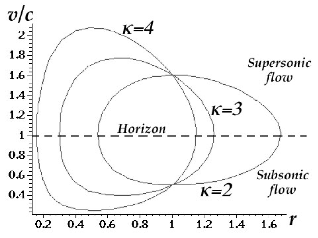
Figure 3: Plot of the solutions of equation (6.4) for $\kappa=2,3,4$ with $d=3$, $c=1$, $r_{0}=1$, and $v_{0}=1/2$.

The four things to emphasize here are that:

1. Velocities equal to the speed of sound are indeed attained;

2. The gradient $dv/dr$ is indeed infinite at the acoustic horizon;

3. These particular solutions break down at the acoustic horizon and cannot be extended beyond it;

4. The particular solutions we have obtained all exhibit a double-valued behaviour, there is a branch with subsonic flow that speeds up and reaches $v=c$ at the acoustic horizon; and there is a second supersonic branch, defined on the same spatial region, that slows down and reaches $v=c$ at the acoustic horizon. Mathematically, this happens because of the double-valuedness of the Lambert function of negative argument, as already noted in section 6.

7.1.2 $\kappa=0$ (no body force)

If there is no external body force, then $d=1$ is uninteresting (the velocity is constant). If we now look at $d=2$ and higher then equation (5.3) again easily gives us the acceleration of the fluid

$$a=v\;{{\mathrm{d}}v\over{\mathrm{d}}r}=-v^{2}\;{c^{2}{(d-1)/r}\over c^{2}-v^{2}}\;,$$ (7.10)

so

$${{\mathrm{d}}v\over{\mathrm{d}}r}=-v\;{c^{2}{(d-1)/r}\over c^{2}-v^{2}}.$$ (7.11)

Explicit integration leads us to the solution

$$r=r_{0}\;\left(\frac{v}{v_{0}}\right)^{\frac{1}{1-d}}\exp\left(\frac{v^{2}-v^{2}_{0}}{2(d-1)c^{2}}\right),$$ (7.12)

which is equivalent to equation (7.3) in the limit $\kappa=0$. This can be easily plotted for different values of the dimension $d$ as shown in figure 4.

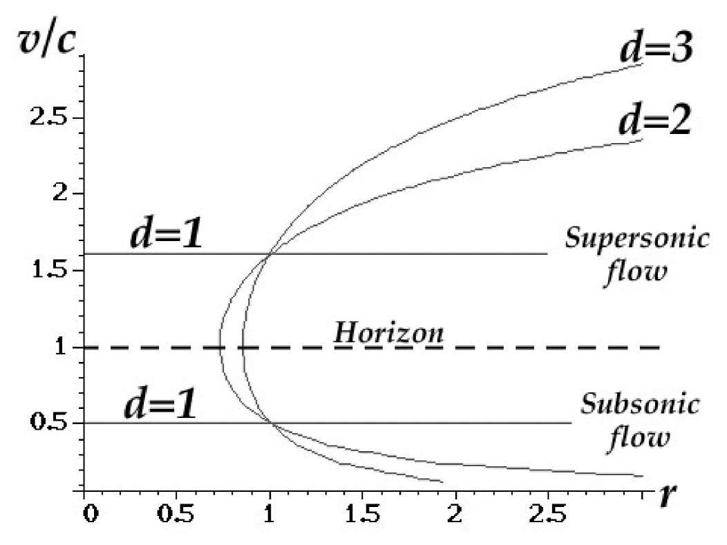
Figure 4: Plot of the solution of equation (6.4) for $\kappa=0$ with the same initial values. ($c=1$, $r_{0}=1$, and $v_{0}=1/2$.) Note the triviality of the $d=1$ solution, which exhibits two branches, with subsonic and supersonic speeds respectively.

7.1.3 $\kappa<0$

For $\kappa<0$ the solutions are plotted in figure 5.

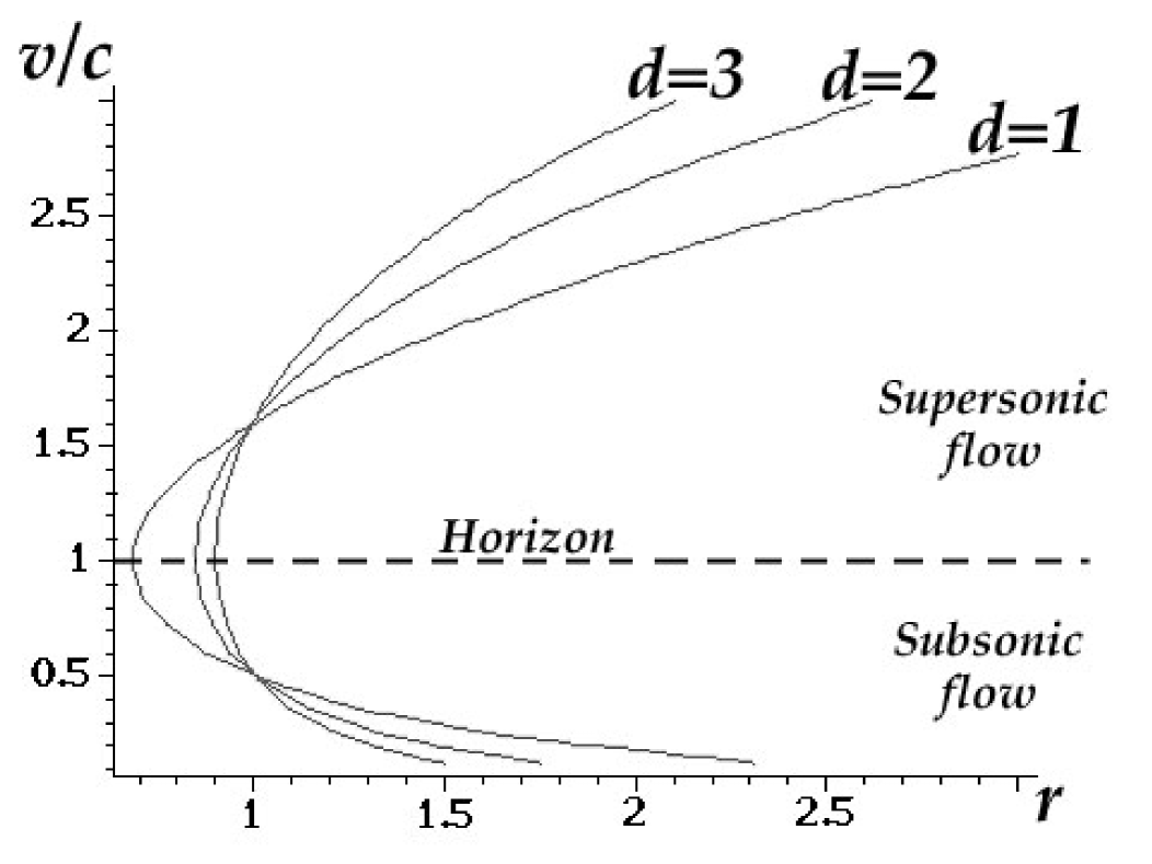
Figure 5: Plot of the solution of equation (6.4) for $d=1,2,3$, and $\kappa=-c^{2}/r_{0}$, where we again set $c=1$, $r_{0}=1$, and $v_{0}=1/2$.

Finally it is interesting to compare the behaviour of the solutions for the different signs of the body force as shown in figure 6.

In all three cases ($\kappa>0$, $\kappa=0$, $\kappa<0$) we see that the acoustic horizon does in fact form as predicted, and that the surface gravity and acceleration are indeed infinite at the acoustic horizon. Naturally, this should be viewed as evidence that some of the technical assumptions usually made are no longer valid as the horizon is approached. In particular in the next section (section 8) we shall discuss the role of viscosity as a regulator for keeping the surface gravity finite.

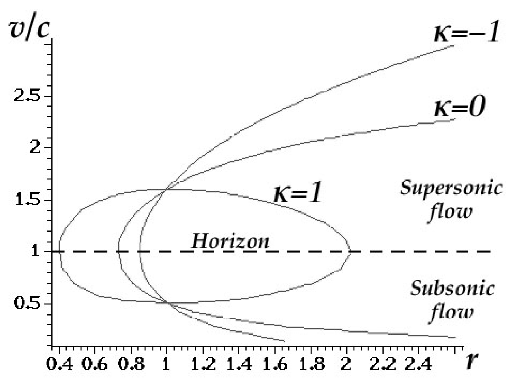
Figure 6: Plot of the solutions of equation (6.4) for $\kappa=\pm 1,0$ and $d=2$, with $c=1$, $r_{0}=1$, and $v_{0}=1/2$.

7.2 Schwarzschild geometry

So far, the discussion in this paper has concerned the attainability of acoustic horizons in general, without focusing on any particular acoustic geometry. A more specific, and rather attractive possibility is to attempt to build a flow with an acoustic metric that is as close as possible to one of the standard black hole metrics of general relativity. Remarkably, this can be done (up to a conformal factor) for the Schwarzschild geometry. To be more specific: for a fluid with constant speed of sound, one can find a stationary, spherically symmetric flow in three spatial dimensions, whose acoustic metric is conformal to the Painlevé–Gullstrand form of the Schwarzschild geometry [6]. This possibility has stimulated considerable work concerning the physical realization of an experimental setup that could actually produce such a flow (or, more precisely, a two-dimensional version of it [16]). These particular fluid configurations exhibit a different type of fine-tuning problem than the one we discussed previously. In order to reproduce the Painlevé–Gullstrand line element, the speed of the fluid must have the profile $v=\sqrt{2M/r}$, with $M$ a positive constant. Then, $r_{0}$ and $v_{0}$ must satisfy the relation $r_{0}v_{0}^{2}=2M$, and equation (6.4) allows us to find the external potential needed in order to sustain such a flow in $d$ space dimensions:

$$\Phi(r)=\Phi(r_{0})+{M\over r_{0}}+c^{2}\left(d-{3\over 2}\right)\ln\left({r\over r_{0}}\right)-{M\over r}.$$ (7.13)

Therefore, the potential must be carefully chosen, which will not be easy to do in a laboratory. If one does manage to construct such a potential $\Phi(r)$ it will automatically fulfill the fine-tuning condition (3.9) at the acoustic horizon, $r_{H}=2M/c^{2}$. This is only to be expected, because ${\mathrm{d}}v/{\mathrm{d}}r=-\sqrt{M/2r^{3}}$ blows up only as $r\to 0$. Also, since we know the surface gravity of a Schwarzschild black hole is finite, any fluid flow that reproduces the Schwarzschild geometry must by definition satisfy the fine tuning condition for a finite surface gravity.

Looking at the issue from the point of view discussed at the end of section 6, one expects that, given the potential (7.13), the value $v_{0}=\sqrt{2M/r_{0}}$ is the solution of equations (6.7) and (6.8), while $v(r)=\sqrt{2M/r}$ is the corresponding eigenfunction that is selected by the requirement of having a regular flow. This is indeed the case: Equation (6.7) now gives $r_{H}=2M/c^{2}$ which, substituted into (6.8), leads to the following equation for $v_{0}$:

$${c^{2}\over 2}\,\ln\left({2M\over r_{0}v_{0}^{2}}\right)+{v_{0}^{2}\over 2}={M\over r_{0}}.$$ (7.14)

It is trivial to check that $v_{0}=\sqrt{2M/r_{0}}$ is, in fact, a solution of (7.14).

Considering the same potential (7.13), but values of $v_{0}$ different from $\sqrt{2M/r_{0}}$, corresponds to flows either with no horizon, or in which $({\mathrm{d}}v/{\mathrm{d}}r)_{H}$ diverges. This is evident in figure 7, which confirms the “eigenvalue character” of the problem of finding a regular flow. Notice that there are two solutions that are regular at the horizon, with opposite values of $({\mathrm{d}}v/{\mathrm{d}}r)_{H}$, in full agreement with the fact that equation (6.2) only determines the square of $({\mathrm{d}}v/{\mathrm{d}}r)_{H}$.

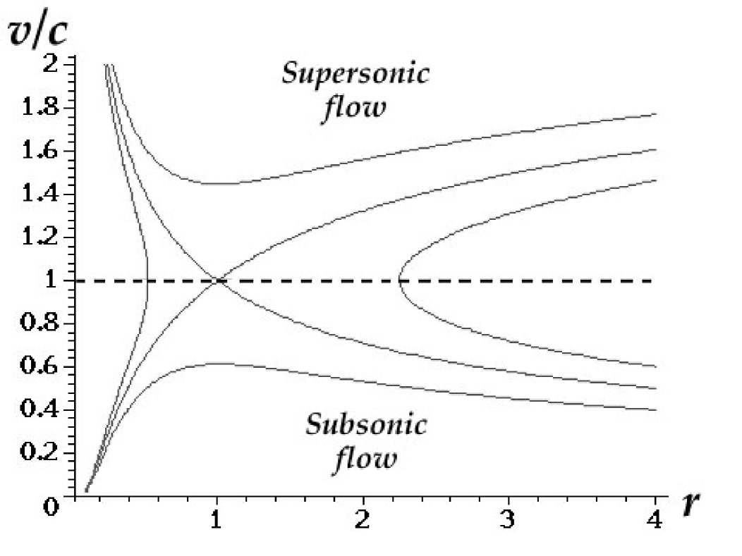
Figure 7: Plot of the solutions of equation (6.4) for the potential (7.13), with $M=1/2$, $d=3$, $c=1$, and $r_{0}=4$. The corresponding boundary conditions are $v_{0}=0.4$, $v_{0}=0.5$, and $v_{0}=0.6$.

Additionally, note that what we have done above has been to ask how to mimic a slice of the $(3+1)$-dimensional Schwarzschild geometry with a $(d+1)$-dimensional fluid flow. We could ask what happens in different spacetime dimensions: for the $(D+1)$-dimensional generalization of the Schwarzschild geometry the fluid flow generalizes to $v=\sqrt{2M/r^{D-2}}$, and the potential gradient required to produce this flow is

$$\Phi(r)=\Phi(r_{0})+{M\over r_{0}^{D-2}}+c^{2}\left(d-{D\over 2}\right)\ln\left({r\over r_{0}}\right)-{M\over r^{D-2}}.$$ (7.15)

Again a very specific external body force is needed to set up the very specific fluid flow corresponding to a higher-dimensional Schwarzschild geometry.

7.3 Reissner–Nordström geometry

We mention in passing that generalizing this discussion to the $(3+1)$-dimensional Reissner–Nordström geometry is straightforward. This geometry is described in Painlevé–Gullstrand form by the fluid flow

$$v(r)=\sqrt{{2M\over r}-{e^{2}\over r^{2}}}.$$ (7.16)

The external potential required to set up this fluid flow is then

$$\Phi(r)=c^{2}\left(d-{3\over 2}\right)\ln\left({r\over r_{0}}\right)-{M\over r}+{e^{2}\over 2r^{2}}+{c^{2}\over 2}\ln\left(1-{e^{2}\over 2Mr}\right)+\mbox{const}.$$ (7.17)

7.4 The canonical acoustic black hole

To wrap up our section on specific examples, we add a few words about the “canonical” acoustic black hole discussed in [6, 8]. In that model the fluid is assumed to have a constant density throughout space, and the continuity equation is then used to deduce the velocity profile

$$v(r)\propto 1/r^{2}.$$ (7.18)

Note that “constant density” is actually a much weaker statement than incompressibility, and the word incompressible should be excised from all of section 8 of [6] and replaced by this phrase. Now in [6, 8] the velocity profile was determined purely on these kinematic grounds, and no attempt was made to put this background fluid flow back into the Euler equations to determine the external body force required to set up the flow. (In that paper, almost all the attention was focussed on the fluctuations rather than the background flow.)

Determining the potential is an easy application of the general analysis of this article [see equation (5.7)]. We calculate

$$\Phi(r)\propto-1/r^{4}+\mbox{const}.$$ (7.19)

With hindsight this can be seen to be nothing more than a special case of Bernoulli’s theorem for a constant-density flow

$$\Phi(r)=-{1\over 2}\;v^{2}+\hbox{const}.$$ (7.20)

The single over-riding message coming from all these specific examples is the generic dichotomy between a formally infinite surface gravity and needing a highly specific boundary condition to be satisfied. In the following section we shall regulate the generically infinite surface gravity by using a less idealized model for the fluid.

8 Viscosity

A viscous flow is governed by the Navier-Stokes equation (2.4). In general, there will be two contributions to viscosity, associated with the coefficients $\eta$ and $\zeta$. Since our treatment in the present section does not pretend to be realistic, but we simply wish to point out how viscosity acts as a regulator for the surface gravity, we shall set the bulk viscosity coefficient $\zeta$ to zero, in order to have a model with as few free parameters as possible. (This is sometimes called the “Stokes assumption” [25].) For a spherically symmetric inflow one has

$$\vec{n}\cdot\left(\nabla^{2}{\vec{v}\,}+{1\over 3}\,\vec{\nabla}\vec{\nabla}\cdot{\vec{v}\,}\right)={4\over 3}\,\left({{\mathrm{d}}^{2}v\over{\mathrm{d}}r^{2}}+{(d-1)\over r}{{\mathrm{d}}v\over{\mathrm{d}}r}-{(d-1)v\over r^{2}}\right),$$ (8.1)

so the Navier-Stokes equation (2.4) becomes, in the stationary case,

$$a=v\;{{\mathrm{d}}v\over{\mathrm{d}}r} = -{v^{2}\over c^{2}-v^{2}}\;\left[{c^{2}(d-1)\over r}-{{\mathrm{d}}\Phi\over{\mathrm{d}}r}\right.$$ (8.2)

$$+ \left.{4\nu\over 3}\left({{\mathrm{d}}^{2}v\over{\mathrm{d}}r^{2}}+{(d-1)\over r}{{\mathrm{d}}v\over{\mathrm{d}}r}-{(d-1)v\over r^{2}}\right)\right],$$

where we have introduced the coefficient of kinematic viscosity $\nu=\eta/\rho$. Hereafter we assume, for simplicity, that $\nu$ is a constant. (However, any hypothesis about $\nu$ must ultimately by justified by a kinetic model for the fluid, and it is worth noticing that there are plausible distribution functions that lead to a velocity-dependent $\nu$; see, e.g., [27]. Obviously, such a dependence can have important repercussions on the conclusions of the present section.) The acceleration is then infinite at the horizon unless

$$\left(1-{4\nu\over 3cr_{H}}\right){c^{2}(d-1)\over r_{H}}-\left.{{\mathrm{d}}\Phi\over{\mathrm{d}}r}\right|_{H}+{4\nu\over 3}\left(\left.{{\mathrm{d}}^{2}v\over dr^{2}}\right|_{H}+{(d-1)\over r_{H}}\left.{{\mathrm{d}}v\over{\mathrm{d}}r}\right|_{H}\right)=0.$$ (8.3)

Since this involves higher-order derivatives at the horizon, it can no longer be regarded as a fine-tuning constraint, or as an equation for $r_{H}$, but merely as a statement about the shape of the velocity profile near the horizon. Indeed the general solution to this equation when $c$ is constant is

$$v(r) = c+{a_{H}\over c}(r-r_{H})+{(d-1)\over 2cr_{H}}\left({c^{2}\over r_{H}}-a_{H}\right)(r-r_{H})^{2}$$ (8.4)

$$+ {3\over 8\nu}\left(\left.{{\mathrm{d}}\Phi\over{\mathrm{d}}r}\right|_{H}-{c^{2}(d-1)\over r_{H}}\right)(r-r_{H})^{2}+O\left((r-r_{H})^{3}\right),$$

with $a_{H}$ arbitrary, and finite, at the horizon. We can rearrange (8.2) to get a differential equation for $v(r)$:

$${{\mathrm{d}}^{2}v\over{\mathrm{d}}r^{2}}+\left({(d-1)\over r}+{3\over 4\nu}{c^{2}-v^{2}\over v}\right){{\mathrm{d}}v\over{\mathrm{d}}r}-{(d-1)v\over r^{2}}={3\over 4\nu}\left({{\mathrm{d}}\Phi\over{\mathrm{d}}r}-{c^{2}(d-1)\over r}\right).$$ (8.5)

Unfortunately, integrating this equation is completely impractical in general and we must resort to the analysis of special cases.

8.1 $d=1$, constant body force

Even the case of constant body force is intractable unless $d=1$, in which case we get (following the steps above)

$${{\mathrm{d}}v\over{\mathrm{d}}r}=-{v\over c^{2}-v^{2}}\left(-\kappa+{4\nu\over 3}{{\mathrm{d}}^{2}v\over{\mathrm{d}}r^{2}}\right).$$ (8.6)

This single second-order differential equation can be turned into an autonomous system of first-order equations

$$\left\{\begin{array}[]{lll}\displaystyle{\frac{{\mathrm{d}}v}{{\mathrm{d}}r}}&=&\Pi,\\ &&\\ \displaystyle{\frac{{\mathrm{d}}\Pi}{{\mathrm{d}}r}}&=&\displaystyle{\frac{3\kappa}{4\nu}+\frac{3v}{4\nu}\left(1-\frac{c^{2}}{v^{2}}\right)\Pi}.\end{array}\right.$$ (8.7)

We can plot the flow of this autonomous system in the usual way and it clearly shows that it is possible to cross the acoustic horizon $v=c$ at arbitrary accelerations $a_{H}$ and arbitrary surface gravity $g_{H}$ (see figure 8).

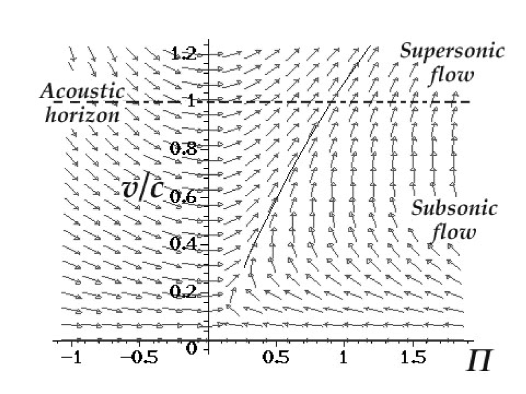
Figure 8: Plot of the phase space for $d=1$, $\kappa=\mbox{constant}>0$, and nonzero viscosity. The transverse line identifies a separatrix in the integral curves. Note that the integral curves can intersect the acoustic horizon at arbitrary values of the surface gravity.

8.2 $d=1$, zero body force

Integrating equation (8.6) once (this is easy provided $c$ is a constant), we get

$$\left.{{\mathrm{d}}v\over{\mathrm{d}}r}\right|_{r}=\left.{{\mathrm{d}}v\over{\mathrm{d}}r}\right|_{r_{0}}-{3\over 8\nu}\;\left[c^{2}\;\ln\left(\frac{v^{2}}{v^{2}_{0}}\right)-v^{2}+v^{2}_{0}\right]+{3\over 4\nu}\left(\Phi(r)-\Phi(r_{0})\right),$$ (8.8)

where $(r_{0},v_{0})$ again denotes an arbitrary pair of initial values. If $d=1$ and $\kappa=0$ this equation for ${\mathrm{d}}v(r)/{\mathrm{d}}r$ reduces to

$$\left.{{\mathrm{d}}v\over{\mathrm{d}}r}\right|_{r}=\left.{{\mathrm{d}}v\over{\mathrm{d}}r}\right|_{r_{0}}-{3\over 8\nu}\;\left[c^{2}\;\ln\left(\frac{v^{2}}{v^{2}_{0}}\right)-v^{2}+v^{2}_{0}\right].$$ (8.9)

In this particular case the analysis is sufficiently simple that we can say something about the acceleration at the horizon, namely

$$\left.{{\mathrm{d}}v\over{\mathrm{d}}r}\right|_{H}=\left.{{\mathrm{d}}v\over{\mathrm{d}}r}\right|_{r_{0}}-{3\over 8\nu}\;\left[c^{2}\;\ln\left(\frac{c^{2}}{v^{2}_{0}}\right)-c^{2}+v^{2}_{0}\right].$$ (8.10)

That is

$$g_{H}=a_{H}=c\left.{{\mathrm{d}}v\over{\mathrm{d}}r}\right|_{r_{0}}-{3c\over 8\nu}\;\left[c^{2}\;\ln\left(\frac{c^{2}}{v^{2}_{0}}\right)-c^{2}+v^{2}_{0}\right],$$ (8.11)

which is an explicit analytic verification that viscosity regularizes the surface gravity of the acoustic horizon.

We can plot the flow in the usual way and it again clearly shows that it is possible to cross the acoustic horizon $v=c$ at arbitrary accelerations $a_{H}$ (see figure 9).

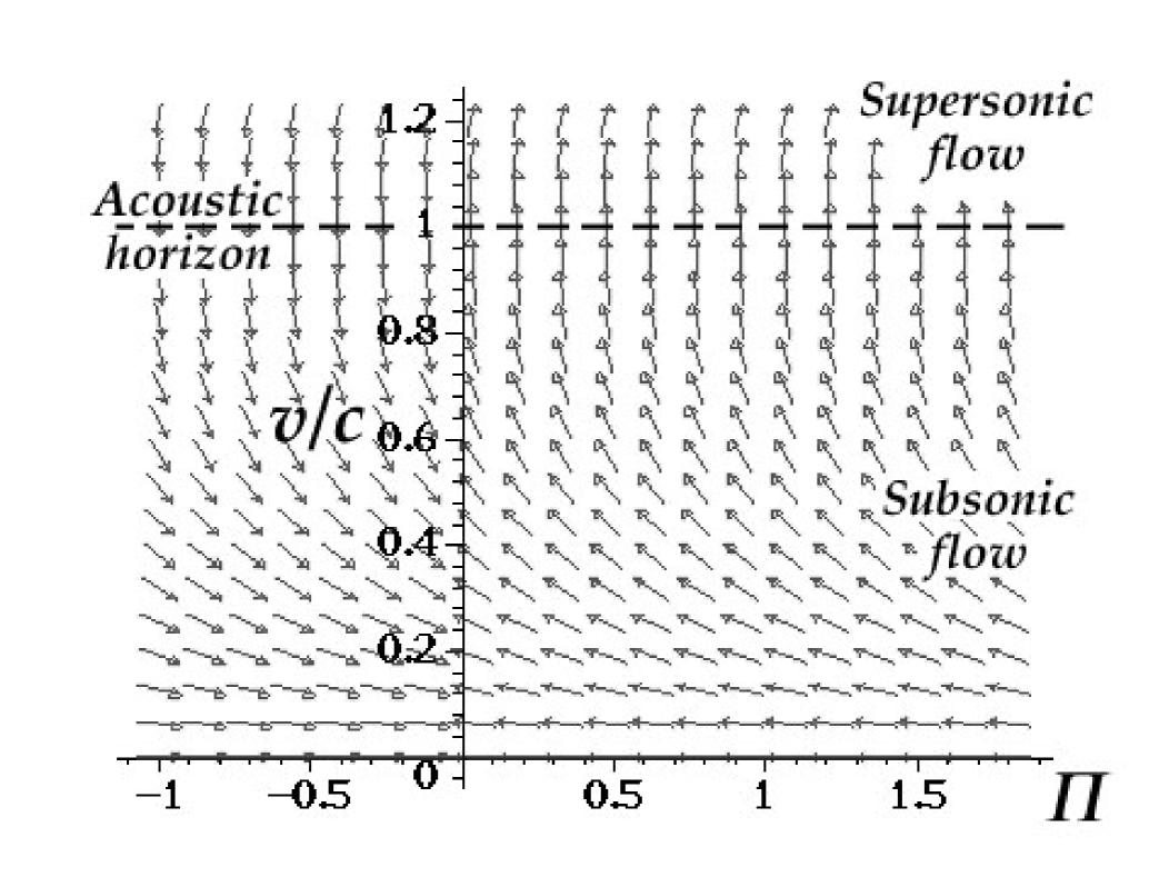
Figure 9: Plot of the phase space for $d=1$, $\kappa=0$, and nonzero viscosity. Again note that the integral curves can intersect the acoustic horizon at arbitrary values of the surface gravity.

8.3 $d>1$, constant body force

The relevant equation is

$${{\mathrm{d}}^{2}v\over{\mathrm{d}}r^{2}}+\left({(d-1)\over r}+{3\over 4\nu}{c^{2}-v^{2}\over v}\right){{\mathrm{d}}v\over{\mathrm{d}}r}-{(d-1)v\over r^{2}}={3\over 4\nu}\left(\kappa-{c^{2}(d-1)\over r}\right),$$ (8.12)

which can be recast as

$$\left\{\begin{array}[]{lll}\displaystyle{{{\mathrm{d}}v\over{\mathrm{d}}r}}&=&\Pi\\ &&\\ \displaystyle{\frac{{\mathrm{d}}\Pi}{{\mathrm{d}}r}}&=&{\displaystyle{3\over 4\nu}\left(\kappa-\frac{c^{2}(d-1)}{r}\right)+{(d-1)v\over r^{2}}+\left(\frac{3v}{4\nu}\left(1-\frac{c^{2}}{v^{2}}\right)-{(d-1)\over r}\right)\Pi}.\end{array}\right.$$ (8.13)

This is no longer an autonomous system of differential equations, (there is now an explicit $r$ dependence in these equations) so a flow diagram is meaningless. Nonetheless the system can be treated numerically and curves plotted as a function of initial conditions. As an example we plot some curves in the phase space for $d=2$, and verify that at least some of these curves imply formation of an acoustic horizon.

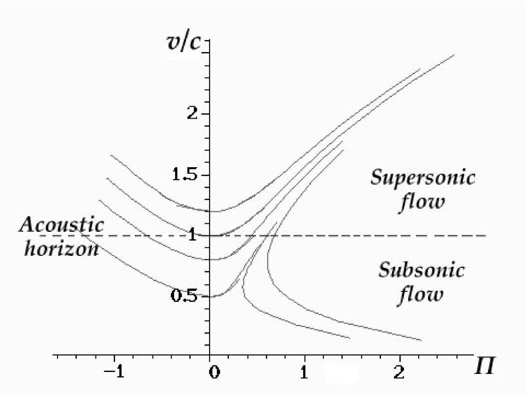
Figure 10: Plot of some solutions to the non-autonomous system (8.13) for various initial conditions for $d=2$, $\kappa=\mbox{constant}$, and nonzero viscosity. Note that at least some of these curves intersect the acoustic horizon, and do so at various but finite values of the surface gravity.

As a final remark we think it is useful to briefly discuss the effect of viscosity with regard to Hawking radiation. It has been shown that the addition of viscosity to the fluid dynamical equations is equivalent to the introduction of an explicit violation of “acoustic Lorentz invariance” at short scales [6, 7]. Thus one may wonder if such an explicit breakdown would not lead to a suppression of the Hawking flux as well. Indeed the violation of Lorentz invariance is important for wavelengths of order $\lambda_{0}=\nu/c$ [6, 7], introducing in this way a sort of cutoff on short wavelengths which can dramatically affect the Hawking flux [2, 3, 5, 20].

Thus there is naively a risk that using viscosity to remove the unphysical divergences at acoustic horizons would also “kill” the phenomenon one is seeking. This problem has been extensively discussed in the literature (see e.g. [20]) and it has (quite remarkably) been demonstrated that such a violation of Lorentz invariance is not only harmless but even natural and useful. In particular, viscosity can be shown to induce [6, 7] the same type of modifications of the phonon dispersion relation which are actually required for circumventing the above cited problem [2, 3, 5, 20]. So the emergence of viscosity appears to be indeed a crucial factor, both for allowing the formation of acoustic horizons and, at the same time, for implementing that mechanism of “mode regeneration” which permits Hawking radiation in presence of short distance cutoff.

9 Conclusions: Danger+opportunity.

Let us summarize the results that we have obtained for a fluid subjected to a given external potential: In the viscosity-free, stationary case, we have seen that if the flow possesses an acoustic horizon, the gradients of physical quantities, as well as the surface gravity and the corresponding Hawking flux, generically exhibit formal divergences. There are two ways in which a real fluid can circumvent this physically unpalatable result. For a broad class of potentials, there is one particular flow which is regular everywhere, even at the horizon. In this case, it is obvious that the fluid itself will “choose” such a configuration. Mathematically, imposing the regularity condition at the horizon amounts to formulating an eigenvalue problem. However, there are physically interesting potentials — such as a linear one — for which this is impossible. We view this result as both a danger and an opportunity. A danger because infinite accelerations are clearly unphysical and indicate that the idealization of considering a irrotational barotropic inviscid perfect fluid (and this idealization underlies the standard derivations of the notion of acoustic metric [1, 4, 6, 8]), is sure to break down in the neighborhood of any putative acoustic horizon. Indeed, the divergences will be avoided in real life simply because one or more of the simplifying hypothesis become invalid as $v\to c$.

On the other hand, this may be viewed as an opportunity: Once we regulate the infinite surface gravity, by adding for instance a finite viscosity, we find that the surface gravity becomes an extra free parameter, divorced from naive estimates based on the geometry of the fluid flow. The common naive estimates of the surface gravity take the form [1, 8]

$$g_{H}\approx{c^{2}\over R},$$ (9.1)

where $R$ is a typical length scale associated with the flow (a nozzle radius, or the radius of curvature of the horizon). The analysis of this note suggests that this estimate may in general be misleading because it does not take into account information regarding the dynamics of the flow. Because of this the surface gravity could be considerably larger than previously expected.

There is a potential source of confusion which we should clarify before wrapping up: in general relativity the physical acceleration of a stationary observer hovering just outside the black hole horizon diverges, but when an appropriate red-shift factor is applied and the properly defined surface gravity is calculated that surface gravity proves to be finite. On the contrary, in the acoustic black holes it is the Newtonian acceleration of the infalling observers that (in the absence of fine-tuning) diverges at the horizon, leading to an infinite surface gravity. Why the difference? It is here that the actual dynamical equations governing the background geometry come into play. The physics that is identical between gravitational black holes and acoustic black holes is the kinematical physics of fields propagating in the respective Lorentzian spacetime metrics. The physics which is different is that which depends on the dynamical equations of motion of the background geometry. For gravity, the latter is governed by the Einstein equations while for acoustic black holes it is governed by the hydrodynamic equations — these equations are sufficiently different that the geometries of the two Lorentzian metrics can be quite different, even though qualitative features such as the existence of event horizons may be quite similar.

Our general discussion, plus the specific example utilizing viscosity, makes it clear that it is the specific technical restrictions placed on the hydrodynamic equations that lead to the formally infinite surface gravity — and so one might wonder how much of the current analysis to trust. For example, in real superfluids the existence of roton excitations leads to a breakdown of irrotational flow before the acoustic horizon is reached [20]. Adding vorticity is certainly technically complicated (see for instance the recent book by Ostashev [28]), but this may merely be a technical complication, not a fundamental barrier to progress. For technical discussions regarding the possibility (probability) of actually building acoustic black holes see [9, 10, 11, 12, 13, 14, 15, 16, 17, 18, 19, 20]. Note that the Garay et al. implementation of acoustic black holes [19] is built on a different physical background; they use Bose–Einstein condensate governed by the Gross–Pitaevski equation rather than a barotropic fluid governed by the Euler-continuity equations. Therefore the perils and opportunities delineated in this article do not necessarily apply to their particular situation. A similar remark applies to Volovik’s implementation based on two-fluid models of superfluidity (for example ³He-A), where the horizon is defined using the speed of the quasi-particles, rather than by the speed of sound per se. Of these two speeds, the former is much smaller than the latter, so the surface gravity at such horizons is always finite [18]. In short, while specific physical implementations of the acoustic geometry idea all have their characteristic peculiarities and potential pitfalls, overall the experimental prospects continue to look extremely promising.

References

- [1] W.G. Unruh, “Experimental black hole evaporation?” Phys. Rev. Lett. 46, 1351–1353 (1981).
- [2] T.A. Jacobson, “Black hole evaporation and ultrashort distances”, Phys. Rev. D 44, 1731–1739 (1991).
- [3] T.A. Jacobson, “Black hole radiation in the presence of a short distance cutoff”, Phys. Rev. D 48, 728–741 (1993) [hep-th/9303103].
- [4] M. Visser, “Acoustic propagation in fluids: an unexpected example of Lorentzian geometry”, gr-qc/9311028.
- [5] W.G. Unruh, “Sonic analogue of black holes and the effects of high frequencies on black hole evaporation”, Phys. Rev. D 51, 2827–2838 (1995) [gr-qc/9409008].
- [6] M. Visser, “Acoustic black holes: Horizons, ergospheres, and Hawking radiation”, Class. Quantum Grav. 15, 1767–1791 (1998) [gr-qc/9712010].
- [7] M. Visser, “Hawking radiation without black hole entropy”, Phys. Rev. Lett. 80, 3436–3439 (1998) [gr-qc/9712016].
- [8] M. Visser, “Acoustic black holes”, Lecture delivered at the Advanced School on Cosmology and Particle Physics, Peniscola, Spain, June 1998; gr-qc/9901047.
- [9] G.E. Volovik, “Simulation of quantum field theory and gravity in superfluid 3He”, Low Temp. Phys. (Kharkov) 24, 127–129 (1998) [cond-mat/9706172].
- [10] N.B. Kopnin and G.E. Volovik, “Critical velocity and event horizon in pair-correlated systems with “relativistic” fermionic quasiparticles”, Pisma Zh. Eksp. Teor. Fiz. 67, 124–129 (1998) [cond-mat/9712187].
- [11] G.E. Volovik, “Gravity of monopole and string and gravitational constant in 3He-A”, Pisma Zh. Eksp. Teor. Fiz. 67, 666–671 (1998); JETP Lett. 67, 698–704 (1998) [cond-mat/9804078].
- [12] G.E. Volovik, “Induced gravity in superfluid 3He”, J. Low Temp. Phys. 113, 667–680 (1997) [cond-mat/9806010].
- [13] T.A. Jacobson and G.E. Volovik, “Event horizons and ergoregions in 3He”, Phys. Rev. D 58, 064021 (1998).
- [14] T.A. Jacobson and G.E. Volovik, “Effective spacetime and Hawking radiation from moving domain wall in thin film of 3He-A”, Pisma Zh. Eksp. Teor. Fiz. 68, 833–838 (1998); JETP Lett. 68, 874–880 (1998) [gr-qc/9811014].
- [15] G.E. Volovik, “Field theory in superfluid 3He: What are the lessons for particle physics, gravity, and high temperature superconductivity?” Proc. Nat. Acad. Sci. 96, 6042–6047 (1999) [cond-mat/9812381].
- [16] G.E. Volovik, “Simulation of Painlevé–Gullstrand black hole in thin 3He-A film”, Pisma Zh. Eksp. Teor. Fiz. 69, 662–668 (1999); JETP Lett. 69 705–713 (1999) [gr-qc/9901077].
- [17] G.E. Volovik, “3He and universe parallelism”, in Topological defects and the Non-Equilibrium Dynamics of Symmetry Breaking Phase Transitions”, Eds. Y.M. Bunkov and H. Godfrin, Kluwer Academic Publishers, 2000, pp. 353 - 387; [cond-mat/9902171].
- [18] G.E. Volovik, “Links between gravity and dynamics of quantum liquids”, gr-qc/0004049.
- [19] L.J. Garay, J.R. Anglin, J.I. Chirac and P. Zoller, “Black holes in Bose–Einstein condensates”, gr-qc/0002015.
- [20] T.A. Jacobson, “Trans–Planckian redshifts and substance of the spacetime river”, hep-th/0001085.
- [21] H.B. Nielsen and M. Ninomiya, “Beta function in a non-covariant Yang-Mills theory”, Nucl. Phys. B141, 153–177 (1978).
- [22] H.B. Nielsen and I. Picek, “Lorentz non-invariance”, Nucl. Phys. B211, 269–296 (1983).
- [23] S. Chadha and H.B. Nielsen, “Lorentz invariance as a low energy phenomenon”, Nucl. Phys. B217, 125–144 (1983).
- [24] L.D. Landau and E.M. Lifshitz, Fluid Mechanics (Pergamon, Oxford, 1959).
- [25] P.K. Kundu, Fluid Mechanics (Academic, 1990).
- [26] R.M. Corless, G.H. Gonnet, D.E.G. Hare, D.J. Jeffrey and D.E. Knuth, “On the Lambert function”, Adv. Comp. Math. 5, 329–359 (1996).
- [27] R. Narayan, “A flux-limited model of particle diffusion and viscosity”, Ap. J. 394, 261–267 (1992).
- [28] V.E. Ostashev, Acoustics in Moving Inhomogeneous Media (E & FN Spon, Thompson Professional, London, 1997).