Adaptive filtering techniques for gravitational wave interferometric data: Removing long-term sinusoidal disturbances and oscillatory transients.

Abstract

It is known by the experience gained from the gravitational wave detector proto-types that the interferometric output signal will be corrupted by a significant amount of non-Gaussian noise, large part of it being essentially composed of long-term sinusoids with slowly varying envelope (such as violin resonances in the suspensions, or main power harmonics) and short-term ringdown noise (which may emanate from servo control systems, electronics in a non-linear state, etc.). Since non-Gaussian noise components make the detection and estimation of the gravitational wave signature more difficult, a denoising algorithm based on adaptive filtering techniques (LMS methods) is proposed to separate and extract them from the stationary and Gaussian background noise. The strength of the method is that it does not require any precise model on the observed data : the signals are distinguished on the basis of their autocorrelation time. We believe that the robustness and simplicity of this method make it useful for data preparation and for the understanding of the first interferometric data. We present the detailed structure of the algorithm and its application to both simulated data and real data from the LIGO 40meter proto-type.

04.80.Nn, 07.05.Kf, 07.50.Hp, 07.60.Ly

I Introduction

Over the next decade, several large-scale interferometric gravitational wave detectors will come on-line. These include LIGO, composed of two Laser Interferometer Gravitational-wave Observatories situated in the U.S. [1], VIRGO, a French/Italian project located near Pisa [2], GEO600, a German/British interferometer under construction near Hannover [3], TAMA in Japan, a medium-scale laser interferometer [4], and with funding approval AIGO500, the proposed 500 meter project sponsored by ACIGA. There are also separate proposals for space-based detectors which could be operational twenty-five years from now (e.g., LISA: the Laser Interferometer Space Antenna, a cornerstone project of the European Space Agency [5]). In the meantime, a number of existing resonant bar detectors will have had their sensitivities further enhanced.

The key to gravitational wave detection is the very precise measurement of small changes in distance. For laser interferometers, this is the distance between pairs of mirrors hanging at either end of two long, mutually perpendicular vacuum chambers. Gravitational waves passing through the instrument will shorten one arm while lengthening the other. By using an interferometer design, the relative change in length of the two arms can be measured, thus signaling the passage of a gravitational wave at the detector site. Long arm lengths, high laser power, and extremely well-controlled laser stability are essential to reach the requisite sensitivity, since the gravitational waves will be faint and will modify only weakly the structure of space-time in the detector’s arms (see e.g., [6]).

Gravitational wave detectors produce an enormous volume of output (e.g., of the order of 16 MB/sec for the LIGO instruments) consisting mainly of noise from a host of sources both environmental and intrinsic to the apparatus. Buried in this noise will be the gravitational wave signature. Sophisticated data analysis techniques will have to be developed to optimally extract astrophysical data. Many of the techniques developed so far  [7, 8, 9] are based on matched filtering and assume stationary Gaussian noise.

However, the real data stream from the detectors is not expected to satisfy the stationary and Gaussian assumptions. In fact, the data from the Caltech 40 meter proto-type interferometer has the expected broadband noise spectrum, but superposed on this are several other noise features [7]; such as long-term sinusoidal disturbances emanating from suspensions and electric main harmonics and also transients occurring occasionally, typically due to servo-controls instabilities or mechanical relaxation in suspension system etc. While no precise a priori model can be given for this noise until the detector is completed and fully tested, matched filtering techniques cannot be used to locate/remove these noisy signals.

This disparity between standard Gaussian assumptions and real data characteristics poses a major problem to the direct application of matched filtering techniques. This is true when searching for burst sources such as blackhole binary quasinormal ringings [10]. This is also the case for the inspiral searches in Caltech 40meter data, where one has to introduce a veto [7] on the decision taken with the matched filter to ensure that the detected signal is actually the one we are looking for.

It is possible that in the future, improved experimental techniques and greater experience, will reduce or even completely eliminate some of these nonstationary and non-Gaussian features. Nevertheless, it will take probably some time to reach such acceptable and high quality of data. Therefore, it is necessary and desirable to somehow combat this noise. Since such noise features defy modeling, a novel approach to the problem is called for.

We propose a denoising method based on LMS adaptive linear prediction techniques which does not require any precise a priori information about the noise characteristics. Although our method does not pretend to optimality, we believe that its simplicity makes it useful for data preparation and for the understanding of the first data.

In the following, we present the principles of LMS adaptive denoising (Sect. II), a characterization of its behavior on a simple model of the noise from the interferometer (Sect. III), the precise structure of the denoising algorithm (Sect. IV) and results (Sect. V) obtained with simulated data and also with real data taken from the Caltech 40 meter proto-type interferometer [11].

This work here is preliminary; its goal is to explore how effectively adaptive filtering techniques perform on the problem we address. It is a first step towards a more complete statistical evaluation of the algorithm.

II Methods

A From hypothesis to method

We assume that the noise consists of broadband Gaussian noise plus large amplitude oscillating interference signals. The model does not include any a priori knowledge of the signal such as its exact frequency or shape of the envelope. The only assumption we make is that its autocorrelation over a small time-lag – the time-lag chosen greater than the decorrelation time scale of the broadband noise – is appreciable, while for the broadband noise it is essentially zero. This difference can be used to advantage to discriminate between the narrow band interferences and the broadband noise.

The idea is to predict the current signal sample given the previous samples of the data. This is possible, only if the target sample shares enough information with (i.e., is sufficiently correlated to) the previous samples. In other words, the only predictable part of the signal is the one whose correlation length is sufficiently large (i.e., long-term sinusoids or ringdowns). Conversely, broadband noise cannot be predicted, as it is not possible to guess the next value in this way. It is this crucial underlying idea we use to discriminate between the two noise signals.

B Mean square linear prediction

Let us recall some standard principles to design an optimal linear predictor. The question to address is to optimally predict the data sample $x_{k}$ with a collection of past samples $\boldsymbol{x}_{k}:=(x_{k-d-m},m=0,1,\ldots,N-1)^{t}$ given the delay $d\geq 1$ (the quantity $d$ is also referred to as prediction depth). The prediction is obtained by linearly combining these data samples weighted by the $N$ corresponding coefficients $w^{(m)}$, forming the tap-weight vector $\boldsymbol{w}:=(w^{(m)},m=0,1,\ldots,N-1)^{t}$, where the superscript ‘t’ denotes the transpose of the vector. Therefore, the prediction $y_{k}$ of $x_{k}$ reads,

$$y_{k}:=\boldsymbol{w}^{t}\boldsymbol{x}_{k}.$$ (1)

The predictor is optimal in the mean square sense when the variance of the prediction error $e_{k}=x_{k}-y_{k}$ is minimum. Therefore, the problem is to find the set of weight coefficients which minimizes

$$J_{k}(\boldsymbol{w}):=\mbox{E}[e^{2}_{k}]=\mbox{E}[(x_{k}-\boldsymbol{w}^{t}\boldsymbol{x}_{k})^{2}],$$ (2)

where E denotes the expectation value operator.

This leads to the minimization of the following quadratic form

$$J_{k}(\boldsymbol{w})=\sigma^{2}_{k}-2\boldsymbol{w}^{t}\boldsymbol{p}_{k}+\boldsymbol{w}^{t}\boldsymbol{R}_{k}\boldsymbol{w},$$ (3)

where $\sigma^{2}_{k}:=\mbox{E}[x^{2}_{k}]$, $\boldsymbol{p}_{k}:=\mbox{E}[x_{k}\boldsymbol{x}_{k}]$ and $\boldsymbol{R}_{k}:=\mbox{E}[\boldsymbol{x}_{k}^{t}\boldsymbol{x}_{k}]$. There exists only one solution $\boldsymbol{w}^{*}_{k}$, obtained when the gradient of $J_{k}$ vanishes. This situation is realized when

$$\boldsymbol{R}_{k}\boldsymbol{w}^{*}_{k}=\boldsymbol{p}_{k}.$$ (4)

When the signal is stationary, $\boldsymbol{R}_{k}=\boldsymbol{R}$ and $\boldsymbol{p}_{k}=\boldsymbol{p}$ are constant (independent of $k$). In this case, $\boldsymbol{R}$ defines the autocorrelation matrix of the signal $x_{k}$ and the solution of (4) is referred to as the Wiener filter.

C Linear prediction and LMS method

Eq. (4) requires the computationally expensive inversion of the matrix $\boldsymbol{R}_{k}$. An alternative and more efficient solution for finding the minimum of the (3) consists in starting from an arbitrary initial value $\boldsymbol{w}_{k,0}$, and iterate the tap-weight vector along the steepest descent direction,

$$\boldsymbol{w}_{k,n+1}=\boldsymbol{w}_{k,n}-\mu\nabla_{\boldsymbol{w}}J_{k}(\boldsymbol{w}_{k,n}),$$ (5)

given by the gradient

$$\nabla_{\boldsymbol{w}}J_{k}(\boldsymbol{w})=2(\boldsymbol{R}_{k}\boldsymbol{w}-\boldsymbol{p}_{k}).$$ (6)

For a sufficiently small gain $\mu$, the weight vectors will eventually converge to the optimal predictor filter $\boldsymbol{w}_{k}^{*}$. This procedure requires the second order statistics (namely $\boldsymbol{R}_{k}$ and $\boldsymbol{p}_{k}$) of the signal. In our case, this information is not available and one has therefore to estimate these quantities. Instead of estimating directly $\boldsymbol{R}_{k}$ and $\boldsymbol{p}_{k}$ and combining them with (6), a more efficient solution is to estimate the gradient. From the derivation of (2), one can rewrite the gradient as

$$\nabla_{\boldsymbol{w}}J_{k}(\boldsymbol{w})=-2\mbox{E}[e_{k}\boldsymbol{x}_{k}].$$ (7)

A simple and natural way to obtain an estimator of this quantity is to omit the expectation operator :

$$\widehat{\nabla_{\boldsymbol{w}}J_{k}}=-2e_{k}\boldsymbol{x}_{k}.$$ (8)

Because the noise perturbs this estimate, the algorithm may iterate in a direction which does not lie along the direction of steepest descent, thus preventing the filter from converging to the Wiener filter. For this purpose, we stabilize the estimation above by setting the algorithm time index $n$ equal to signal time index $k$ in the Eq. (5). The final evolution equation for the tap-weight vector finally reads:

$$\boldsymbol{w}_{k+1}=\boldsymbol{w}_{k}+2\mu e_{k}\boldsymbol{x}_{k}.$$ (9)

At a fixed time $k$, the weight vector evolves along the crude estimate of the steepest descent direction. But on a longer duration, the direction followed by the tap-weight vector is governed by the sum of the successive gradient estimates obtained with different noise samples. In other words, we have replaced an ensemble average in (7) by a time average. It also implies that we have implicitly called for further assumptions on the signal $x_{k}$: first its local stationarity (more precisely, the second order statistics are supposed to be constant during the convergence time of the algorithm) and second, its ergodicity.

Summarizing, the method we propose consists in linearly filtering the data to extract the part of the signal with a long correlation time. As illustrated with the block diagram in Fig. 1, the finite impulse response filter (given by $\boldsymbol{w}_{k}$) is modified at each iteration according to the relation (9) with the final goal to minimize the mean square error. Once the filter has converged (i.e., $\boldsymbol{w}_{k}$ is stable in time), we reject the predicted part of the signal (corresponding to the long-term sinusoidal or the ringdown signals) and we send the rest of the signal for further analysis for detection.

D Properties of the LMS method

The method we described above is referred to as adaptive line enhancer (ALE). It is a special case of the LMS algorithm. Both, ALE and LMS algorithms have been first introduced by Widrow and Hoff [12] in the 1960’s.

The acronym LMS (Least Mean Square) designates a general scheme to design signal processing methods where a minimization (in a statistical sense) of a definite positive quadratic cost function (usually related to some mean quadratic error) is needed. Its central idea is the use of the estimate of the gradient of this function given in Eq. (8). The LMS technique has been extensively used for the last 30 years in communications problems such as echo cancellation, channel equalization, antenna processing, etc. The main advantages to be gained by applying the LMS technique are (i) adaptivity, (ii) robustness, (iii) simplicity.

In this context, the term “adaptivity” has two different meanings. First, it means that the LMS technique will automatically modify its parameters to reach for the best setup for a problem which has not been initially precisely defined. Second, it is also able to follow changes in the characteristics of the data being processed in the event that they occur. The latter property also shows that the method is robust. In fact, this method has been proved to be robust according to specific statistical criterion such as the minimax criterion [13].

The ALE is an adaptive prediction algorithm using the LMS technique. We have seen that the signal is predicted from a reference signal which is the signal itself. In some other applications, although the same principles are applied, the reference signal can be another signal, e.g. echo cancellation or denoising. In such cases, the quantity of interest might not be the prediction output but the linear filter used to compute it, e.g., deconvolution.

III Adapting ALE filter to canceling noise in GW data

In this section we essentially describe a model for understanding the behaviour of the ALE algorithm. The model we assume consists of a high amplitude narrowband signal superposed on broadband noise. For simplicity, we assume the broadband noise to be white and Gaussian and the narrowband signals are sinusoids of constant envelope. The results we obtain hold for more realistic signals when the evolution of their amplitude and/or instantaneous frequency occurs adiabatically, i.e., the change is small over the period of the sinusoid.

The assumption of white noise is not too restrictive because this is equivalent to choosing the noise correlation time to be zero and therefore we are free to choose the prediction depth (i.e., the time delay between the current predicted data sample and the reference signal to the LMS filter) to be arbitrarily small. In a real situation, we must fix the delay to be greater than the correlation time of the broadband noise. We first analyze the case of the sinusoid because it is easier to investigate and provides invaluable insights into the workings of the LMS algorithm.

It may be remarked that the denoising of sinusoids in white noise has been treated in the literature with great detail (see [13, 14] for a review). We give here only pertinent results (with a short proof) for introducing the structure of the algorithm, which we present later in the text.

A Optimal filter

We consider the data to be of the following form,

$$x_{k}:=\cos(2\pi f_{0}t_{k}+\Phi)+n_{k},$$ (10)

where $t_{k}:=k\delta$, $\delta:=1/f_{s}$ being the sampling interval and $\Phi$ is a random phase (at the origin) with uniform probability density function between $-\pi$ and $\pi$. The sinusoid has frequency $f_{0}$ and the units are so chosen that it is of unit amplitude. The additive white noise $n_{k}$ with variance $\sigma^{2}$ satisfies the relation,

$$\mbox{E}[n_{k}n_{m}]:=\sigma^{2}\delta_{km},$$ (11)

where $\delta_{km}$ is the Kronecker delta.

The reference signal to the adaptive filter is just the delayed data by the amount $d\delta$, where $d$ is the number of time samples. We choose $N$ weights $w_{k}\equiv W$ ($\boldsymbol{w}$ can be thought of as a column vector) for the length of our filter, then the “reference vector” $\boldsymbol{x}_{k}$ at the $k$th time instant $t_{k}$ has the components $x_{k-d-n}$, $n=0,1,\ldots,N-1$. The components of the autocorrelation matrix $\boldsymbol{R}$ and the vector $\boldsymbol{p}$ in Eq.(3) are given by

$$\boldsymbol{R}^{(mn)} =1/2\cos(m-n)\delta\phi+\sigma^{2}\delta_{mn}$$ (12)

$$\boldsymbol{p}^{(m)} =1/2\cos(m+d)\delta\phi,$$ (13)

where $(m,n)=0,1,\ldots,N-1$ and $\delta\phi=2\pi f_{0}\delta$. Note that we have dropped the index $k$ because the autocorrelation $\boldsymbol{R}$ does not depend upon $k$, since we are dealing with a stationary signal.

From the above expressions of $\boldsymbol{R}$ and $\boldsymbol{p}$ and solving Eq.(4), we obtain the optimum Wiener filter

$$\boldsymbol{w}^{*(m)}=\frac{2}{N+4\sigma^{2}}\,\cos(m+d)\delta\phi,\quad m=0,1,\ldots,N-1.$$ (14)

where we have chosen the length of the filter to be half-integral number of cycles for reasons of simplicity, i.e. $N\delta\phi=l\pi$, where $l$ is an integer.

In other words, the optimum linear predictor is nothing but a copy of the expected signal itself. The filter in Eq. (14) is also referred to as matched filter. In our situation, in practise, $N\gg\sigma^{2}$ and the term $4\sigma^{2}$ can be omitted from the amplitude of $\boldsymbol{w}^{*}$.

For the reasons detailed before, we propose to use the ALE algorithm in order to find a good approximation of $\boldsymbol{w}^{*}$. Starting from an arbitrary initial tap-weight vector, we iterate the weights $\boldsymbol{w}_{k}$ according to Eq. (9) to converge to $\boldsymbol{w}^{*}$. Once the filter is “close” enough to the optimal solution (the word “close” will be defined later in the text), we then say that the filter has locked on to the signal.

B Approach to locking

a Continuous time approximation of the locking trajectory —

We may analyze the approach to locking by deriving a difference equation for the averaged evolution of the weights and then investigating this equation. It is impossible to obtain the average evolution of the weights by using the standard definition of the expectation operator E because of the nonlinearity and the recursive scheme involved in evolving the weights. We therefore adopt the time-average over successive data points as the operational definition of E.

Shifting the origin to $\boldsymbol{w}^{*}$ by defining $\boldsymbol{v}_{k}:=\boldsymbol{w}_{k}-\boldsymbol{w}^{*}$, we may write the LMS evolution equation (9) in the following form [15]:

$$\boldsymbol{v}_{k+1}-\boldsymbol{v}_{k}=-2\mu(\boldsymbol{x}_{k}\boldsymbol{x}_{k}^{t})\boldsymbol{v}_{k}+2\mu e_{k}^{*}\boldsymbol{x}_{k},$$ (15)

where $e_{k}^{*}:=x_{k}-\boldsymbol{w}^{*t}\boldsymbol{x}_{k}$ is the prediction error produced when using the optimal filter.

During the locking phase, the filter is far apart from the optimal location (i.e., $\boldsymbol{v}_{k}$ has a large modulus). The homogeneous term dominates the forcing term in the difference equation (15) which then can be approximated by :

$$\boldsymbol{v}_{k+1}-\boldsymbol{v}_{k}=-2\mu(\boldsymbol{x}_{k}\boldsymbol{x}_{k}^{t})\boldsymbol{v}_{k}.$$ (16)

In the situation where the step gain parameter $\mu$ is chosen to be very small so that the weight coefficients are almost constant over a given time interval, the recursivity eventually acts as an averaging operation on both sides of the equation above. This leads to the difference equation which we use to describe the tap-weight trajectory in the space of weight coefficients, we denote ${\cal W}$ :

$$\boldsymbol{v}_{k+1}-\boldsymbol{v}_{k}=-2\mu\boldsymbol{R}\boldsymbol{v}_{k}.$$ (17)

Let $\boldsymbol{Q}$ be the transformation which diagonalizes $\boldsymbol{R}$. The above difference equation is best analyzed by changing the frame in ${\cal W}$ to the principal axis

$$\tilde{\boldsymbol{v}}_{k+1}-\tilde{\boldsymbol{v}}_{k}=-2\mu\tilde{\boldsymbol{R}}\tilde{\boldsymbol{v}}_{k},$$ (18)

where $\tilde{\boldsymbol{R}}:=\boldsymbol{Q}\boldsymbol{R}\boldsymbol{Q}^{-1}={\rm diag}(\lambda^{(0)},\ldots,\lambda^{(N-1)})$ and $\tilde{\boldsymbol{v}}_{k}:=\boldsymbol{Q}\boldsymbol{v}_{k}$. Eq. (18) gives decoupled difference equations for the components $\tilde{\boldsymbol{v}}^{(m)}_{k},m=0,\ldots,N-1$ of $\tilde{\boldsymbol{v}}$ which can be solved given the initial weight vector $\tilde{\boldsymbol{v}}^{(m)}_{0}$ :

$$\tilde{\boldsymbol{v}}^{(m)}_{k}=\tilde{\boldsymbol{v}}^{(m)}_{0}(1-2\mu\lambda^{(m)})^{k}.$$ (19)

b Eigenvalues and eigenvectors of $\boldsymbol{R}$ —

We need to compute the eigenvalues $\lambda^{(m)}$ of $\boldsymbol{R}$. This can be conveniently implemented by splitting $\boldsymbol{R}$ into the noise part, which is just $\sigma^{2}$ times the identity plus the signal part which we denote by $\boldsymbol{S}/2$, and thus,

$$\boldsymbol{R}=\sigma^{2}\boldsymbol{I}+\boldsymbol{S}/2,$$ (20)

where $\boldsymbol{S}^{(mn)}:=\cos(m-n)\delta\phi$. It is easily verified that the eigenvectors of $\boldsymbol{R}$ and $\boldsymbol{S}$ are identical and the eigenvalues of $\boldsymbol{R}$ are obtained from those of $\boldsymbol{S}$ by first halving them and then adding $\sigma^{2}$ to the result. It remains, therefore, to compute the eigenvalues and eigenvectors of $\boldsymbol{S}$. We do this by observing that we can write $\boldsymbol{S}$ as follows :

$$\boldsymbol{S}=(\boldsymbol{\nu}\boldsymbol{\nu}^{\dagger}+\bar{\boldsymbol{\nu}}\bar{\boldsymbol{\nu}}^{\dagger})/2,$$ (21)

where $\boldsymbol{\nu}:=(1,\exp(i\delta\phi),\exp(2i\delta\phi),\ldots,\exp((N-1)i\delta\phi))^{t}$.

Since the matrix $\boldsymbol{S}$ is real and is essentially made out of two external products of $\boldsymbol{\nu}$ and $\bar{\boldsymbol{\nu}}$, its rank equals $2$ ($\boldsymbol{S}$ has $N-2$ degenerate eigendirections in ${\cal W}$ with eigenvalue zero) with two non-zero real eigenvalues. Let $\boldsymbol{v}$ be an eigenvector associated to one of the non-trivial eigenvalues. According to the structure of $\boldsymbol{S}$, the vector $\boldsymbol{v}$ can be written without loss of generality as the following linear combination,

$$\boldsymbol{v}=\boldsymbol{\nu}\,\exp(-i{\alpha})+\bar{\boldsymbol{\nu}}\,\exp(i{\alpha}),$$ (22)

where the coefficients have been chosen to have unit modulus arbitrarily.

Using the two scalar products $\boldsymbol{\nu}^{\dagger}\boldsymbol{\nu}=N$ and

$$\boldsymbol{\nu}^{t}\boldsymbol{\nu} =1+\exp(2i\delta\phi)+\ldots+\exp(2(N-1)i\delta\phi)$$ (23)

$$:=\beta\exp i\gamma,$$ (24)

where the geometric series can be summed up and modulus and phase ascertained :

$$\beta =\frac{\sin(N\delta\phi)}{\sin\delta\phi}$$ (25)

$$\gamma =(N-1)\delta\phi,$$ (26)

we obtain the effect of the matrix $\boldsymbol{S}$ on the vector $\boldsymbol{v}$, given by

$$\boldsymbol{S}\boldsymbol{v}=\boldsymbol{\nu}\,\exp(-i{\alpha})(N+\beta\exp(-i\gamma+2i{\alpha}))/2+c.c.$$ (27)

where c.c. denotes complex conjugate.

This expression has to be compared to the second term of the eigenvalue equation $\boldsymbol{S}\boldsymbol{v}=\lambda\boldsymbol{v}$, leading to two solutions for ${\alpha}$, namely, ${\alpha}=\gamma/2$ and ${\alpha}=(\gamma-\pi)/2$. These yield the eigenvectors $\boldsymbol{v}_{\pm}$ and the corresponding eigenvalues $\lambda_{\pm}$ :

$$\begin{array}[]{rcl}\boldsymbol{v}_{+}&=&\boldsymbol{\nu}\exp(-i\gamma/2)+\bar{\boldsymbol{\nu}}\exp(i\gamma/2),\\[5.69054pt] \boldsymbol{v}_{-}&=&i\boldsymbol{\nu}\exp(-i\gamma/2)-i\bar{\boldsymbol{\nu}}\exp(i\gamma/2),\end{array}$$ (28)

$$\lambda_{\pm}=(N\pm\beta)/2.$$ (29)

If we choose $N$ large enough and $N\delta\phi=m\pi$, where $m$ is an integer then the analysis becomes simpler. This amounts to choosing the length of the filter to have half-integral number of cycles: we have $\beta=0$ and $\lambda_{\pm}=N/2$. (Geometrically, this means that the eigenvalue problem is degenerate with respect to the two signal eigenvectors: there is a two dimensional eigenspace belonging to the eigenvalue $N/2$. The weights thus evolve non-preferentially with respect to the signal eigendirections.) Since typical cases imply generally $N\gg\beta$, we will assume this simplification in the rest of the paper.

In this situation, the spectrum of $\boldsymbol{R}$

$$\mbox{sp}(\boldsymbol{R})=\{\lambda^{(0)}=\lambda^{(1)}=N/4+\sigma^{2}\quad\text{ and }\\ \lambda^{(m)}=\sigma^{2},m=2,\ldots,N-1\},$$ (30)

consist of two sets of eigenvalues : the first two correspond to directions in the signal space associated to “signal+noise” (or “signal”, for short) whereas the remaining $N-2$ characterize “noise” directions.

According to Eq. (19), the weight vector will converge more rapidly in directions associated with the largest eigenvalues, which are the signal eigenvalues. The other noise eigenvalues are unimportant in this consideration. The eigenvectors pertaining to the signal provide preferred directions in ${\cal W}$: it is along these directions that the slope of the performance surface is steep and hence promotes faster convergence.

C Steady state evaluation

If the step gain factor is sufficiently small, the tap-weight coefficients eventually converge and stabilize in a neighbourhood of the optimal value. At this stage, the assumptions made in obtaining the approximated evolution equation (17) do not hold anymore. In contrast with the case of “the approach to locking”, the right hand side of the difference equation (15) is now dominated by the forcing term :

$$\boldsymbol{v}_{k+1}-\boldsymbol{v}_{k}=2\mu e_{k}^{*}\boldsymbol{x}_{k}.$$ (31)

Roughly speaking, the trajectory of the vector $\boldsymbol{w}_{k}$ during the steady state can be viewed as a random walk centered around $\boldsymbol{w}^{*}$ lying within a region of ${\cal W}$ space whose extent is determined by two factors, namely, $\mu$ and the intrinsic geometry of ${\cal W}$ in the vicinity of $\boldsymbol{w}^{*}$.

The misalignment between the actual ALE filter $\boldsymbol{w}_{k}$ and the optimal one $\boldsymbol{w}^{*}$ creates an additional error in the output. In fact, a direct calculation from Eq. (3) shows that the total mean square error may decomposed as [12] :

$$J_{k}(\boldsymbol{w}_{k})=\xi_{min}+\xi_{k},$$ (32)

where (i) $\xi_{min}:=J_{k}(\boldsymbol{w}^{*})$ is the minimum mean square error arising from the fraction of the input noise which still remains in the output, assuming that the ALE filter has reached exact optimality and (ii) $\xi_{k}:=\boldsymbol{v}_{k}^{t}\boldsymbol{R}\boldsymbol{v}_{k}$ is the excess mean square error (EMSE) due to the misalignment between the ALE filter and the Wiener filter.

One can verify that the EMSE vanishes when reaching optimality i.e., when $\boldsymbol{v}_{k}=\boldsymbol{0}$. In other words, this term quantifies the non optimality of the current filter in use. We can imagine $\xi_{k}$ as the square of a natural distance in ${\cal W}$ and $\boldsymbol{R}$ as a intrinsic metric over ${\cal W}$.

A good approximation of $\xi_{min}$ can be found for large number of weight coefficients for the specific case of sinusoidal signals with high SNRs. Using Eqs. (3) and (4), we may write $\xi_{min}=\mbox{E}[x_{k}^{2}]-\boldsymbol{p}^{t}\boldsymbol{w}^{*}$. When $N\rightarrow\infty$, a direct calculation shows that the second term $\boldsymbol{p}^{t}\boldsymbol{w}^{*}$ tends to the energy of the sinusoid, which means that the remaining energy is that of the noise:  $\xi_{min}\approx\sigma^{2}$.

We complete the characterization of the mean square error (32) with the evaluation of the average value of the EMSE, which we denote by $\xi^{(st)}$. Firstly, noticing that the EMSE is invariant under the principal axis transformation

$$\xi_{k}=\tilde{\boldsymbol{v}}_{k}^{t}\tilde{\boldsymbol{R}}\tilde{\boldsymbol{v}}_{k}=\sum_{m=0}^{N-1}\lambda^{(m)}\left(\tilde{\boldsymbol{v}}^{(m)}_{k}\right)^{2},$$ (33)

and secondly, using the approximation $\mbox{E}[\tilde{\boldsymbol{v}}_{k}\tilde{\boldsymbol{v}}_{k}^{t}]\approx\mu\xi_{min}\boldsymbol{I}$ proposed in [12] to obtain the typical value for $(\tilde{\boldsymbol{v}}^{(m)}_{k})^{2}$ yields

$$\xi^{(st)}\approx\mu\sum_{m=0}^{N-1}{\lambda^{(m)}}\xi_{min}.$$ (34)

Since the signal is of much larger amplitude than the broadband noise, the trace of $\tilde{\boldsymbol{R}}$ is essentially due to the signal eigenvalues (see Eq. 30). Combining with the expression of $\xi_{min}$ above, this leads to :

$$\xi^{(st)}\approx\mu N\sigma^{2}/2.$$ (35)

A better estimate of $\xi^{(st)}$ can be obtained starting with more realistic hypotheses and using more sophisticated approximations [14] :

$$\xi^{(st)}\approx\sum_{m=0}^{N-1}\frac{\mu\lambda^{(m)}}{1-\mu\lambda^{(m)}}\xi_{min}.$$ (36)

In the limit of small step size, this approximation tends to the simpler one in Eq. (35).

D Convergence time

In the expression of the EMSE in Eq. (33), we separate the sum into two parts: the first, $\xi^{(n)}_{k}$ associated with the noise (i.e., consisting of terms involving noise eigenvalues and vectors), the second, $\xi^{(s)}_{k}$ with the signal. Because the signal eigenvalues are much larger than those of the noise, the sum in Eq. (33) is essentially dominated in the beginning (for small $k$) by $\xi^{(s)}_{k}$. These two errors decrease during the locking phase until reaching a steady state value. The locking time (i.e., time at which the steady state is reached) is defined to be that, when $\xi^{(s)}_{k}$ is of the order of the total EMSE expected in the steady state.

From Eqs. (19), (29) and (33) we obtain,

$$\xi^{(s)}_{k} :=\lambda^{(0)}\left(\tilde{\boldsymbol{v}}^{(0)}_{k}\right)^{2}+\lambda^{(1)}\left(\tilde{\boldsymbol{v}}^{(1)}_{k}\right)^{2}$$ (37)

$$\approx\frac{N}{4}\left(\left(\tilde{\boldsymbol{v}}_{0}^{(0)}\right)^{2}+\left(\tilde{\boldsymbol{v}}_{0}^{(1)}\right)^{2}\right)\left(1-\frac{\mu N}{2}\right)^{2k},$$ (38)

where we have assumed $N\gg\beta$.

We set the starting point $\boldsymbol{w}_{0}$ in ${\cal W}$ to be $\boldsymbol{0}$. It corresponds to the initial value $\tilde{\boldsymbol{v}}_{0}$ in the eigenspace which is given by $\tilde{\boldsymbol{v}}_{0}=-\boldsymbol{Q}\boldsymbol{w}^{*}$. The first two coordinates of $\tilde{\boldsymbol{v}}_{0}$ can be directly obtained since the first two row vectors of $\boldsymbol{Q}$ are just the normalized signal eigenvectors of the $\boldsymbol{R}$ matrix, leading to, for half integral wavelength filters and $N\gg\sigma^{2}$,

$$\tilde{\boldsymbol{v}}^{(0)}_{0} =\sqrt{2/N}\cos(d\delta\phi+\gamma/2)$$ (39)

$$\tilde{\boldsymbol{v}}^{(1)}_{0} =\sqrt{2/N}\sin(d\delta\phi+\gamma/2).$$ (40)

These considerations yield

$$\xi^{(s)}_{k}\approx\frac{1}{2}\left(1-\frac{\mu N}{2}\right)^{2k}.$$ (41)

This error must now be compared with the averaged EMSE in Eq. (35) in order to find the time $t_{\rm lock}$ at which $\xi^{(s)}$ and $\xi^{(st)}$ are equal :

$$t_{\rm lock}\approx\delta\frac{\ln(\mu N\sigma^{2})}{2\ln(1-\mu N/2)}.$$ (42)

It is important to mention that, when the product $\mu N/2$ tends to $1$, the convergence time diverges to infinity meaning that the weights do not converge toward $\boldsymbol{w}^{*}$ anymore. In order to ensure the stability of the algorithm, the parameters will have to satisfy the stability condition $0<\mu N/2<1$. However, we have observed in our simulations that when $1/2\leq\mu N/2<1$, the convergence is slowed down, because of the presence of oscillatory terms in the gradient which do not average to zero anymore. In practise, it is advisable to choose the parameters so that $\mu N/2<1/2$.

For a sinusoid of amplitude $A$ instead of unity as we have considered before, the condition for stability can be simply obtained by replacing the parameter $\mu N/2$ by $\rho:=\mu NA^{2}/2$ leading to $0<\rho<1$.

We illustrate in Figs. 2 and 3 with an example the results of this Section pertaining to the approach to locking and steady state analysis.

IV The ALE in practice

In the previous Sections we have characterized the behaviour of the ALE in cases of interest. We will now elaborate on how this algorithm can be adapted to the interferometric data.

In the scheme we present here, we first decompose the signal in $p$ frequency subbands to which we apply the ALE twice with different sets of parameters. In the first stage, the parameters are tuned to best remove long-term sinusoidal components of the noise; whereas in the second stage, the target consists of shorter oscillatory transients.

A Subband decomposition

Interferences such as mains power and violin mode harmonics are distributed over a large dynamic scale (the first harmonics are of much larger amplitude than those of high order). But, since the interferometer noise curve also decreases at low frequencies, their relative amplitude as compared to the background noise power spectrum at the same frequency remains large. Therefore, the model introduced previously, namely that of large amplitude sinusoidal signals embedded in broadband noise, is a reasonable approximation within the relevant small bandwidth of frequencies.

For this reason, we divide the frequency axis in $p$ disjoint frequency subbands of the same size. The $p$ signals lying in each of the subbands are heterodyned and decimated to the sampling frequency $f_{s}^{\textrm{band}}:=f_{s}/p$.

The tiling has the advantage that, if $p$ is sufficiently large, we can consider the interferometer background noise almost white within a subband, which implies that the noise has vanishing correlation time. The prediction depth $d$ which has to be larger than the correlation time, can be then simply fixed to any value greater than $1$ sample period in each of the subbands.

B Long-term sinusoid removal

Certain parts of the spectrum may not contain any long-term periodic interferences. We apply a preliminary test to exclude subbands which may not require the first denoising step. The test is crudely done by estimating the amplitude $A$ of the sinusoid from the largest peak of the power spectrum (Welch estimate) and comparing it to the variance $\sigma^{2}$ of the broadband noise (also estimated from the power spectrum). If it is found that $A>\sigma$, we decide that there exists a long-term sinusoidal signal of sufficient amplitude in the band which needs to be removed, otherwise we proceed directly to the second step.

We apply the ALE in each of the selected subbands choosing parameters as follows:

• Number of tap-weight coefficients $N$
  The number of tap-weight coefficients is fixed by prescribing an upperbound $0<\eta_{noise}<1$ to the ratio between the noise power corrupting the filtered output $y_{k}$ of the optimal filter $\boldsymbol{w^{*}}$ and the input noise power. Let $\boldsymbol{n}_{k}:=(n_{k-d-m},m=0,1,\ldots,N-1)^{t}$ be a collection of noise samples, then the above condition reads ,

  $$\mbox{E}[(\boldsymbol{w}^{*t}\boldsymbol{n}_{k})^{2}]\leq\eta_{noise}\mbox{E}[(n_{k})^{2}],$$ (43)

  which, with the stationarity and whiteness of the background noise $n_{k}$, results in bound on the optimal filter gain :

  $$\boldsymbol{w}^{*t}\boldsymbol{w}^{*}\leq\eta_{noise}.$$ (44)

  The $L^{2}$ norm $\lVert\boldsymbol{w}^{*}\rVert_{2}^{2}=(2/N^{2})(N+\beta\cos(\gamma+2d\delta\phi))$ is obtained by squaring and summing the Eq. (14) for the optimal filter. Since in typical cases $\beta\ll N$, this leads to simpler expression $\lVert\boldsymbol{w}^{*}\rVert^{2}_{2}\approx 2/N$.

  Consequently, the number of tap-weight coefficients $N$ has to be chosen so that,

  $$N\geq 2/\eta_{noise}.$$ (45)

• Step gain parameter $\mu$
  We fix the step gain parameter by imposing to the distance of the ALE filter from optimality in the steady state to be smaller than a given threshold on average. As we have seen in Sect. III C, this can be done naturally by imposing an upperbound $0<\eta_{sig}<1$ on the excess square mean error as compared to the signal power $E_{s}=A^{2}/2$ :

  $$\xi^{(st)}\leq\eta_{sig}E_{s}.$$ (46)

  Using the expression obtained in the steady state analysis in Eq. (35) for the EMSE, this condition reduces to :

  $$\mu\leq\eta_{sig}/(N\sigma^{2}).$$ (47)

  Generally, this equation leads to small values of $\mu$ which prevent the convergence of the ALE filter from its initial state (i.e., all tap-weight coefficients are fixed to $0$) in a reasonable time (convergence faster than a tenth of second, which is the duration of the chunk of data). We solve this problem by first applying the ALE on a sequence of training data, the step gain parameter being set at the beginning to a large value (for fast convergence) and decreased gradually to the value given in Eq. (47). The filter obtained after the completion of this training is close to the objective (i.e., the Wiener filter). We then start the longterm sinusoid removal using this prepared filter.

  We remark here that although $\mu$ is small, it is non-zero thus giving the ALE filter some flexibility of adapting to changes (non-stationarities) in the signal such as slow drifts in frequency and amplitude modulation. This property, however, needs to be investigated more in detail.

C Ringdown removal

The aim of the second step of the algorithm is to remove oscillatory transients (ringdowns) of large amplitude. These transients are either frequency bands excited from time to time (caused by dysfunctions in the interferometer) or relics from the previous step (when the envelope of a long-term sinusoid possesses fast variations to which the algorithm cannot adapt or converge to during the first step of removal).

The cleaning procedure consists in applying ALE the second time to each of the subbands but now, the parameters are so adjusted that, (i) they select features with a larger bandwidth than in the previous step, and (ii) converge rapidly onto an oscillatory noisy signal that may appear.

• Number of tap-weight coefficients $N$
  The impulse response duration and frequency selectivity (i.e., the filter bandwidth $\Delta f$) of the transfer function are dual in character. This follows from the uncertainty relation. The rough approximate relation between these quantities is given by,

  $$N=f_{s}/(p\Delta f),$$ (48)

  where $f_{s}$ is the sampling frequency. We choose the number of tap-weight coefficients $N$ by imposing a minimum bandwidth $\Delta f_{min}$ to the filter and using the above equation.

• Step gain parameter $\mu$
  Assuming that the ringdown can be locally approximated by a sinusoid, we choose the step gain parameter by imposing a convergence time of the order of a typical transient duration (i.e., $t_{lock}\approx N\delta$). More concretely, setting $\rho:=\mu NA^{2}/2$ in the unnormalized form of Eq. (42) (i.e., for arbitrary ringdown amplitude $A$), we solve for

  $$\frac{\ln(2\sigma^{2}\rho)}{2\ln(1-\rho)}=N.$$ (49)

  Using the crude estimate $A^{2}/2\approx\lVert\boldsymbol{x}_{k}\rVert_{2}^{2}/N$ for the ringdown amplitude, the step gain parameter is finally obtained as $\mu=\rho/\lVert\boldsymbol{x}_{k}\rVert_{2}^{2}$.

Since the ringdown signals are of short duration and can occur with large time gaps, the ALE does not need to operate on each data segment. Accordingly, we have added a supervision test which decides whether or not the denoising algorithm should be applied to a given data segment. The test consists of observing the Gaussianity of the filtered output $y_{k}=\boldsymbol{w}_{k}^{t}\boldsymbol{x}_{k}$. If the input signal $x_{k}$ is a zero-mean white Gaussian process of variance $\sigma^{2}$, then the output of the filter $y_{k}$ shares the same characteristics, except that the variance gets multiplied by the filter gain : $\mbox{var\,}y_{k}=\lVert\boldsymbol{w}_{k}\rVert^{2}_{2}\sigma^{2}$. Furthermore, under this hypothesis, the envelope ${\cal Y}_{k}=\lvert{\cal H}(y)_{k}\rvert^{2}$ (${\cal H}$ denotes the discrete Hilbert transform of $y_{k}$) follows by definition a chi-square distribution with $1$ degree of freedom.

This implies that, up to an arbitrary probability $P_{0}$, the envelope ${\cal Y}_{k}$ does not exceed the threshold given below:

$${\cal Y}_{k}<\kappa(P_{0})\,2f_{s}^{band}\lVert\boldsymbol{w}_{k}\rVert_{2}^{2}\sigma^{2},$$ (50)

where $\kappa(\cdot)$ is the inverse function of the (unit variance) $\chi^{2}$ cumulative distribution function (cdf).

If Eq. (50) is satisfied, we conclude that the filtered output is essentially due to a Gaussian background noise and we leave the input signal as it is. Otherwise, we conclude that the filtered output carries a ringdown signal and decide to remove it from the input data.

The functioning of the second step of the denoising algorithm could be interpreted as follows : it removes from the input data, regions in the time-frequency plane presumably associated with transients, whose support is defined along the frequency axis by the ALE filter, and along the time axis by the supervision criterion (50).

After completing these two steps, we recombine the signal in all the subbands together to retrieve a single strain signal.

V Numerical results

A Simulated data: test of the ringdown removal

In this section, the goal is to test how effectively the second stage of the denoising algorithm (i.e., the ringdown removal) described in Sect. IV operates on a simple signal. The test signal is composed of three ringdown signals (of fixed amplitude and frequency) occurring successively in the data stream and embedded in a additive Gaussian white noise. This model may be used to represent ringdown disturbances originating from the same underlying physical mechanism.

Each of these ringdown signals is a sinusoidal waveform, similar to Eq. (10) (with $A=1$, $f_{0}=50$ Hz and sampling frequency $f_{s}=200$ Hz), whose support is limited in time by a Gaussian envelope :

$$r_{k}:=A\exp\left(-\pi(t_{k}-t_{c})^{2}/T^{2}\right)\,\cos(2\pi f_{0}t_{k}+\Phi),$$ (51)

where three different reference times $t_{c}$ are given and the equivalent time duration is $T=200$ms (giving a frequency bandwidth of $\Delta f\approx 1/T=5$ Hz and $Q:=f_{0}T\approx 10$ cycles).

Figure 4 describes the application of the denoising algorithm configured with $d=5$ sampling periods (equal to $25$ ms) $\Delta f_{min}=3$ Hz, and $P_{0}=0.01$. It can be seen that the algorithm operates better on the transient encountered later in the data train than its predecessor. The explanation is that a transient duration is too short for the filter to reach the steady state but, when it encounters the next transient, the filter benefits from the distance to $\boldsymbol{w}^{*}$ previously covered, thus improving the convergence towards optimality.

This can be verified with a time-frequency representation [16] of the output signal such as Fig. 4, where we have chosen the spectrogram $S_{x}^{h}[n,m]:=|F_{x}^{h}[n,m]|^{2}$ defined as the squared modulus of the short-time Fourier transform :

$$F_{x}^{h}[n,m]:=\sum_{k}{x_{n}h_{k-n}e^{-2\pi inm}},$$ (52)

where $n\in[1,2,\ldots,N]$, $m\in]-1/2\ldots 1/2]$ and $h_{k}$ is an arbitrary window (a Gaussian window here).

Notice that real time and frequency coordinates can be retrieved through the relations : $t=n/f_{s}$ and $f=mf_{s}$.

B Results on Caltech 40m proto-type data

Here we have applied the algorithm to the Caltech 40meter proto-type data taken in October 1994 [11]. This data was recorded with a sampling frequency of $f_{s}=9.86$kHz. We have used the calibrated strain signal [17] (relative arm length measurement) for applying our algorithm.

We tile the complete spectrum into $p=32$ frequency subbands of approximately $154$ Hz each. Each subband encounters typically one or two long-term sinusoidal interferences.

We have chosen the prediction depth to be $d=5$ sampling periods, which corresponds to a delay of $pd/f_{s}\approx 16$ ms in real time. The correlation time of the broadband noise is effectively smaller in each subband except at the extremities of the spectrum where the steep slope of the spectrum does not allow us to assume the background noise to be locally white. It only affects the first and last subbands which are not too important for detection purposes.

In the first stage, we have chosen $\eta_{noise}=0.01$ (giving $N=200$ according to Eq. (45)) and $\eta_{sig}=0.01$. In the second stage of ringdown removal, the minimum filter bandwidth has been fixed to $\Delta f_{min}=3$ Hz, which gives a filter with $N=100$ tap-weight coefficients (see Eq. (48)) and we have set $P_{0}=0.01$ for the Gaussianity test.

We have performed two types of simulations:

• a “Caltech signal only” simulation to measure improvements after denoising : we check firstly, whether the frequency peaks are removed from the noise power spectrum and secondly, whether the noise statistics is closer to Gaussian than before denoising,

• a “Caltech+inspiral” simulation to evaluate the consequences of the denoising algorithm on gravitational wave detection; specifically, for the case of the inspiralling compact binary signal. The question here is to check whether the denoising operation has removed a significant part or even whole of the inspiral signal.

Caltech signal only — Eleven of the thirty-two frequency subbands (# $1$–$9$, $11$ and $17$) are selected and sent to the first cleaning step of the algorithm. In these subbands, we obtained the following mean values for $A\approx 1.5\times 10^{-16}$ and $\sigma\approx 3.6\times 10^{-17}$ (the sinusoid amplitude $A$ equals approximately $1$ to at most $5$ times the noise standard deviation $\sigma$) leading to typical values for the signal-to-noise ratio of about $\mbox{SNR}=A^{2}/(2\sigma^{2})\approx 8.7(9.4\mathsf{dB})$ and for the step gain parameter (see Eq. (47)) of $\mu NA^{2}/2\approx 0.04$ (spanning from $0.01$ to $0.14$).

The complete set of subband signals is processed in the second step. The typical noise variance estimate is $\sigma=1.35\times 10^{-17}$ (from $4.8\times 10^{-18}$ to $10^{-16}$) leading according to Eq. (49) to values of $\mu N\sigma^{2}$ which span the range of values from $0.07$ to $10^{-4}$.

Figure 5 illustrates how the algorithm operates in the fifth frequency subband (from $617$ Hz to $771$ Hz) among the $p=32$ ones being processed. This frequency band contains two power line harmonics (the $11$th at $660$ Hz and the $12$th at $720$ Hz).

Figures 6 and 7 show respectively comparisons between the power spectra and histograms of the signal before and after denoising. We observe that after denoising, the frequency peaks have been removed from the input signal and the histogram appears much closer to the Gaussian bell curve.

Caltech signal + inspiral waveform — The purpose of this test is to evaluate how the cleaning operation affects gravitational wave detection and in particular to make sure whether a significant part of the gravitational signature could be removed from data. Answering this question by analytical means is difficult, however a qualitative rational in the case of inspiral binaries can be made and verified with simulations.

The theory predicts [18] that the gravitational waves emitted from inspiralling binaries of neutron stars are oscillating waveforms whose frequency evolves in time in a prescribed manner and scans the interferometer bandwidth from lower end to the higher.

Their weak amplitude and short time duration within a single subband (in the case we have considered, less than a second) make them “invisible” to the ALE filter. The amplitude and the duration of the gravitational wave signal are simply not large enough for the ALE coefficients to converge onto the gravitational wave instantaneous frequency.

We have checked the validity of this argument by adding to the Caltech signal the inspiralling ‘chirp’ waveform in the Newtonian approximation [18] of two neutron star binaries each having a mass of $M=1.4$ solar masses, and located at a distance of $r=7\,$kpc from the Earth.

Figure 8 depicts a comparison of matched filter detector response on the same signal with and without denoising. The detector output displays a peak of the same height and at the correct instant, showing that the cleaning algorithm has not removed the inspiral signal from the data. This can be crosschecked in Fig. 9 showing a zoomed view of the same signal after denoising.

VI Concluding remarks

The originality of the idea of the proposed denoising algorithm lies in its wide applicability, so that both types of disturbances, long-term sinusoidal and oscillatory transients (the type of noise which has been ignored till now) can be treated. Although the question of the computational burden in applying this algorithm has not quite been addressed here, it appears from the simplicity of the operations involved (e.g., no requirement such as long-term FFTs) that the total computational cost should be within acceptable limits, so that the algorithm can be operated in real time. Furthermore, the structure of the algorithm already implemented with Matlab [19] can be easily translated into a parallel code (each processing node can be associated with one frequency subband and the processing can be done independently).

As part of future extensions to the present work, some improvements to the current code might be needed : in order to limit the finite size effects in the subband decomposition and reconstruction, a reversible filter bank (e.g., a Gabor transform) would be preferable than the crude method used here.

The key idea (i.e., looking for correlation between the current sample of the strain signal and a reference signal, namely a set of past samples) can be also extended to investigate correlations of the detector output with other environmental channels by simply using them as a reference rather than the strain signal itself. Similarly to the cross-talk removal in [20] but with adaptive methods, such an algorithm would provide an estimation of any poorly known (linear) transfer functions relating noise sources to their final leaking in the detector output and of the environmental contamination that must be subtracted from the data, if so desired.

Acknowledgments

We would like to thank B. F. Schutz for suggesting the idea of adaptive methods and also for fruitful conversations and the LIGO collaboration for providing us the Caltech 40meter proto-type data. E. C.-M. would like to thank W. Anderson, R. Balasubramian, J. Creighton and S. Mohanty for their useful comments and suggestions.

FIG. 1.: The figure illustrates the principle of the underlying method on which the algorithm we propose is based. The algorithm is designed to discriminate the nonstationary and non-Gaussian noise features from the broadband background noise in interferometric gravitational wave data. This method is referred to as LMS adaptive line enhancement and its objective is to compare the signal and its linear prediction, the predictor coefficients being adjusted by a feedback loop controlled by the prediction error.

FIG. 2.: Applying the ALE to a sinusoidal signal: approach to locking and steady state. The figure illustrates how the ALE performs on a test signal composed of a sinusoid ($f_{0}=50$ Hz sampled at $f_{s}=1$ kHz) corrupted by white noise (SNR$=A^{2}/(2\sigma^{2})=50(17\mathsf{dB})$). We initialize the $N=40$ tap-weight coefficients to $0$, set the prediction depth $d=5$ (ms) and the step gain parameter $\mu=0.003$. (a): the filter output signal $y_{k}$ (solid line) converges rapidly towards the actual noise free sinusoidal signal (dashed line). (b): this is confirmed by observing that the “signal” EMSE $\xi^{s}_{k}$ defined in Eq. (37) which decreases with time until it reaches its steady state value. For comparison, the horizontal dashed line indicates the theoretical mean value of the total EMSE $\xi^{st}$ in the steady state (see Eq. (35)). We can verify that the theoretical value obtained in Eq. (42) for the convergence time $t_{lock}$ corresponds effectively to the time instant at which $\xi^{s}_{k}$ and $\xi^{st}$ are of the same order. Finally, the two contour plots of the bottom line display the trajectory followed by the adaptive filter coefficients in the eigen weight space : in (c), the axis are the first two eigenvectors of $\boldsymbol{R}$ namely $\tilde{\boldsymbol{v}}_{k}^{(0)}$ and $\tilde{\boldsymbol{v}}_{k}^{(1)}$ (i.e., the “signal” eigenvectors) whereas in (d) the diagram plane is given by $\tilde{\boldsymbol{v}}_{k}^{(1)}$ and $\tilde{\boldsymbol{v}}_{k}^{(2)}$ (i.e., a “signal” direction vs. a “noise” direction). As proved in Sect. III B, the weight coefficients converge more rapidly along the two directions $\tilde{\boldsymbol{v}}_{k}^{(0)}$ and $\tilde{\boldsymbol{v}}_{k}^{(1)}$ given by eigenvectors associated with the largest eigenvalues.

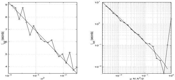
FIG. 3.: Applying the ALE to a sinusoidal signal: convergence time. The figure shows the comparison between the convergence time $t_{lock}$ obtained by simulations (solid line with ’+’ associated with one noise realization) and its theoretical value (solid line) given in Eq. (42). The test signal is a sinusoid in white Gaussian noise (see Eq. (10) with $A=1$, $f_{0}=50$ Hz, sampled at $f_{s}=200$ Hz). The convergence time is shown as a function of $\sigma^{2}$ in (a) (we have fixed the remaining ALE parameters to $N=200$ and $\mu NA^{2}/2=0.01$) and in (b) as a function of $\mu NA^{2}/2$ ($N=200$ and $\sigma^{2}=0.1$). Simulations globally confirm the results obtained in Eq. (42) except when $1/2\leq\mu NA^{2}/2<1$. The reason for this discrepancy is that the difference between the actual gradient (7) and its estimates (8) can be shown to be an oscillating term which does not average to zero any longer when the step gain parameter approaches the critical value for stability. Therefore, in practise, we choose parameters so that $\mu NA^{2}/2<1/2$.

FIG. 4.: Applying the ALE to oscillating transients : testing the ringdown removal algorithm. The figure depicts the results of the transient removal algorithm presented in Sect. IV C to a signal in (a) composed of three successive oscillating bursts (see text for details) embedded in Gaussian white noise (SNR$=A^{2}/(2\sigma^{2})=8(9\mathsf{dB})$). In addition to the ALE, we measure the deviations of the filtered output from Gaussianity : when its envelope (c) exceeds some threshold (dashed line, see Eq. (50)), we decide that the filtered output is not normally distributed and, therefore contains a transient which has to be removed (this is indicated by dots at the top of the graph). The final net effect of the operation is that of time variant filtering of the input data. The corresponding transfer function is represented in (d) : the regions indicated with dark colours are parts of the time-frequency plane where the data are selected and removed from the input (i.e., it corresponds to the time-frequency “band” pass of the filter). Comparing the spectrograms [21] (see Eq. (52) for a definition) in (b) and (f) respectively of the input and output (e) signals, we observe that the three transients are progressively removed from the input (dark regions represent large values of the time-frequency energy density).

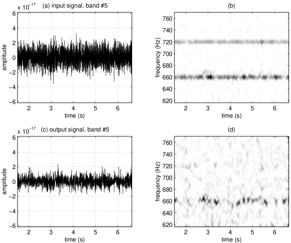
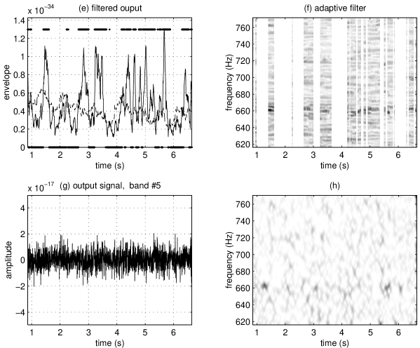
FIG. 5.: Illustration of the denoising procedure on Caltech proto-type data. In the subband #5 (between 617 Hz and 771 Hz), the signal [17] (the data were taken on the October, 14th 1994, frame #2) in (a) contains two power line harmonics (at 660 Hz and 720 Hz), which we are seen as darkened horizontal lines in the spectrogram (see Eq. (52)) in (b). We apply ALE the first time to suppress long-term components (c) with corresponding spectrogram (d). A second run (g) supervised by the criterion (50) detailed in (e) and (f) (see the similar plots in Fig. 4, (c) and (d) for explanation) eliminates artefacts of shorter duration (such as fast fluctuations in the harmonic envelope). Note that the spectrogram (h) of the final signal presents a homogeneous energy density both in time and frequency directions.

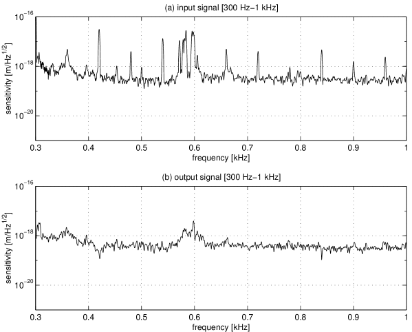
FIG. 6.: “Caltech signal only” : comparison between power spectra of ALE input/output signals. The figure depicts power spectra of the Caltech 40 meter signal (top) in the operating frequency band, between 300 Hz and 1kHz and the same signal after denoising (bottom).

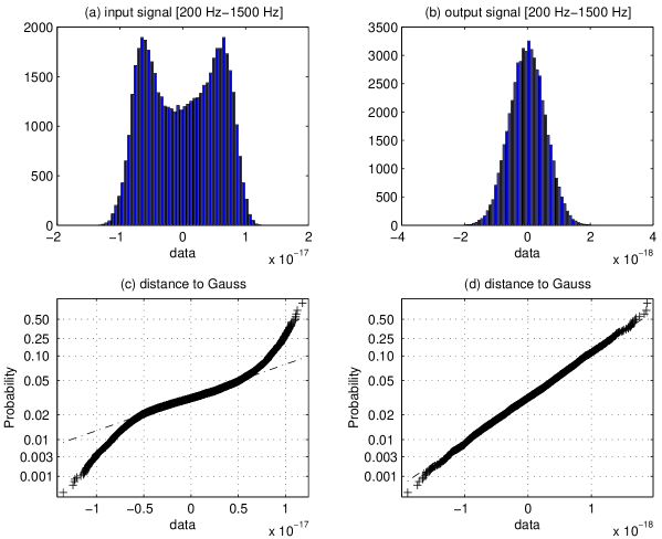
FIG. 7.: “Caltech signal only” : comparison between histograms of ALE input/output signals. The probability density functions of the Caltech 40 meter signal selected between 300 Hz and 1kHz (left column) and the same signal after denoising (right column) have been estimated with histograms (top row). The bottom row shows the same histograms in special axes where a Gaussian bell curve appears as a straight line.

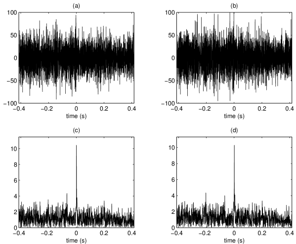
FIG. 8.: “Caltech+inspiral” signal : matched filter response before and after denoising. The Newtonian approximation of a gravitational wave emitted from an inspiraling binary (each with mass $1.4$ solar masses,at a distance of $7$ kpc and coalescence time fixed to $t=0$) has been added to the Caltech interferometric proto-type data. Top row plots show this signal (a) and its corresponding version after denoising (b) which have been selected and whitened within the frequency band $200$ Hz (i.e., the lower frequency bound of the observation window) to $1.3$ kHz (i.e., the predicted frequency for the last stable circular orbit of the binary). The matched filter technique applied to detect the inspiral waveform, shows in both cases (e.g., without (c) and with (d) denoising) a peak at time $t=0$ in their detector responses (the normalization so chosen that “noise only” detector fluctuations are of unit variance).

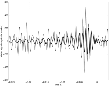
FIG. 9.: “Caltech+inspiral” signal : zoomed view after denoising. As an additional check, this diagram presents a zoomed view at the coalescence time $t=0$ of the signal in Fig. 8-b (whitened signal after denoising). We have superimposed on it (in bold) the signal as it would appear in the noise free case.

REFERENCES

- [1] A. Abramovici et al. LIGO: the laser interferometer gravitational wave observatory. Science, pages 256–325, 1992.
- [2] B. Caron et al. The Virgo interferometer. Class. Quantum Grav., 14(6):1461–1469, 1997.
- [3] H. Lück et al. The GEO600 project. Class. Quantum Grav., 14(6):1471–1476, 1997.
- [4] K. Kudora. In I. Ciufolini and F. Fidecaro, editors, Gravitational Waves: Sources and Detectors. World Scientific, Singapore, 1997.
- [5] K. Danzmann et al. LISA: an ESA cornerstone mission for a gravitational wave observatory. Class. Quantum Grav., 14(6):1399–1404, 1997.
- [6] P. R. Saulson. Fundamentals of Interferometric Gravitational Wave Detectors. World Scientific, Singapore, 1994.
- [7] B. Allen et al. Observational limit on gravitational waves from binary neutron star in the Galaxy. Phys. Rev. Lett., 83(8):1498–1501, 1999.
- [8] S. D. Mohanty. Hierarchical search strategy for the detection of gravitational waves from coalescing binaries: extension to post-Newtonian waveforms. Phys. Rev. D, 57(2):630–658, 1998.
- [9] B. S. Sathyaprakash and S. V. Dhurandhar. Choice of filters for the detection of gravitational waves from coalescing binaries. Phys. Rev. D, 44(12):3819–3834, 1991.
- [10] J. D. E. Creighton. Listening for ringing black holes. gr–qc 9712044, 1997.
- [11] A. Abramovici et al. Improved sensitivity in a gravitational wave interferometer and implication for LIGO. Phys. Letters A, 218:157–163, 1996.
- [12] B. Widrow and S. D. Stearns. Adaptive Signal Processing. Prentice Hall, Englewoods Cliffs, 1984.
- [13] S. Haykin. Adaptive Filter Theory. Prentice Hall, Englewoods Cliffs, third edition, 1996.
- [14] J. R. Zeidler. Performance analysis of LMS adaptive prediction filters. Proc. of the IEEE, 78(12):1781–1806, 1990.
- [15] O. Macchi. Adaptive processing : The Least Mean Square approach with applications in transmission. Wiley, New-York, 1995.
- [16] P. Flandrin. Time-Frequency/Time-Scale Analysis. Academic Press, San Diego (CA), 1999.
- [17] The Caltech signal has been downloaded and calibrated with the GRASP package (version 1.9.3, http://www.lsc-group.phys.uwm.edu).
- [18] K. S. Thorne. Gravitational radiation. In S. W. Hawking and W. Israel, editors, 300 Years of Gravitation, pages 330–458. Cambridge Univ. Press, 1987.
- [19] E. Chassande-Mottin and S. V. Dhurandhar. All Matlab codes which have been used in this document can be freely downloaded at the following address : http://www.aei-postdam.mpg.de/ eric/ale.html.
- [20] B. Allen, W. Hua, and A. Ottewill. Automatic cross-talk removal from multi-channel data. gr–qc 9909083, 1999.
- [21] The spectrograms shown here have been computed with the Time-Frequency Toolbox for Matlab (http://iut-saint-nazaire.univ-nantes.fr/ auger/tftb.html).