Self-similar spherically symmetric cosmological models with a perfect fluid and a scalar field

Abstract

Self-similar, spherically symmetric cosmological models with a perfect fluid and a scalar field with an exponential potential are investigated. New variables are defined which lead to a compact state space, and dynamical systems methods are utilised to analyse the models. Due to the existence of monotone functions global dynamical results can be deduced. In particular, all of the future and past attractors for these models are obtained and the global results are discussed. The essential physical results are that initially expanding models always evolve away from a massless scalar field model with an initial singularity and, depending on the parameters of the models, either recollapse to a second singularity or expand forever towards a flat power-law inflationary model. The special cases in which there is no barotropic fluid and in which the scalar field is massless are considered in more detail in order to illustrate the asymptotic results. Some phase portraits are presented and the intermediate dynamics and hence the physical properties of the models are discussed.

1 Introduction

Scalar field cosmology is of importance in the study of the early Universe and particularly in the investigation of inflation (during which the universe undergoes a period of accelerated expansion [1, 2]). One particular class of inflationary cosmological models are those with a scalar field and an exponential potential of the form $V(\phi)=V_{0}e^{-\kappa\phi}$, where $\kappa$ and $V_{0}$ are constants. Models with an exponential scalar field potential arise naturally in alternative theories of gravity, such as, for example, scalar-tensor theories, and are currently of particular interest since such theories occur as the low-energy limit in supergravity theories [3, 4].

A number of authors have studied scalar field cosmological models with an exponential potential within general relativity. Homogeneous and isotropic Friedmann-Robertson-Walker (FRW) models were first studied by Halliwell [5] using phase-plane methods. Homogeneous but anisotropic models of Bianchi types I and III (and Kantowski-Sachs models) were studied by Burd and Barrow [6] in which they found exact solutions and discussed their stability. Bianchi models of types III and VI were studied by Feinstein and Ibáñez [7], in which exact solutions were found. An analysis of Bianchi models, including standard matter satisfying various energy conditions, was completed by Kitada and Maeda [8, 9]. They found that the well-known power-law inflationary solution is an attractor for all initially expanding Bianchi models (except a subclass of the Bianchi type IX models which will recollapse) when $\kappa^{2}<2$.

The governing differential equations in spatially homogeneous Bianchi cosmologies containing a scalar field with an exponential potential reduce to a dynamical system when appropriate normalised variables are defined; this dynamical system was studied in detail in [10]. In a follow-up paper [11] the isotropisation of the Bianchi VII_h cosmological models possessing a scalar field with an exponential potential was further investigated; in the case $\kappa^{2}>2$, it was shown that there is an open set of initial conditions in the set of anisotropic Bianchi VII_h initial data such that the corresponding cosmological models isotropise asymptotically. Hence, spatially homogeneous scalar field cosmological models having an exponential potential with $\kappa^{2}>2$ can isotropise to the future. The Bianchi type IX models have also been studied in more detail [12].

Recently, cosmological models which contain both a perfect fluid and a scalar field with an exponential potential have come under heavy analysis [13]. One of the exact solutions found for these models has the property that the energy density due to the scalar field is proportional to the energy density of the perfect fluid, hence these models have been labelled scaling cosmologies [14]. These scaling solutions, which are spatially flat isotropic models, are of particular physical interest. For example, in these models a significant fraction of the current energy density of the Universe may be contained in the scalar field whose dynamical effects mimic cold dark matter. In [15] the stability of these cosmological scaling solutions within the class of spatially homogeneous cosmological models with a perfect fluid subject to the equation of state $p=(\gamma-1)\mu$ (where $\gamma$ is a constant satisfying $0<\gamma<2$) and a scalar field with an exponential potential was studied. It was found that when $\gamma>2/3$, and particularly for realistic matter with $\gamma\geq 1$, the scaling solutions are unstable; essentially they are unstable to curvature perturbations, although they are stable to shear perturbations. Curvature scaling solutions [16] and anisotropic scaling solutions [17] are also possible. In particular, in [16] homogeneous and isotropic spacetimes with non-zero spatial curvature were studied.

Clearly it is of interest to study more general cosmological models, and in this paper we shall comprehensively study the qualitative properties of the class of self-similar spherically symmetric models with a barotropic fluid and a non-interacting scalar field with an exponential potential. Self-similar spherically symmetric perfect fluid models with a linear equation of state have been much studied in general relativity [18, 19]. Carr & Coley [20] have presented a complete asymptotic classification of such solutions and, by reformulating the field equations for these models, Goliath et al [21, 22] have obtained a compact three-dimensional state space representation of the solutions which leads to another complete picture of the solution space. Recently, these models have been further studied in a combined approach [23]. The present analysis can be thought of as a natural extension of this recent work [21, 22, 23].

The Kantowski-Sachs models appear as a limiting case of the class of spherically symmetric models under investigation, and hence this analysis complements recent analyses of spatially homogeneous Bianchi models [13]. Models with positive spatial curvature have attracted less attention than Bianchi models with zero spatial curvature or negative spatial curvature since they are more complicated mathematically. However, the properties of positive-curvature FRW models [5, 16, 24] and Kantowski-Sachs models [6] have been studied previously.

In the next section we shall describe the governing equations of the class of models under investigation. In section 3, compact variables are defined and the resulting dynamical system is derived in the case of spatial self-similarity. A monotone function is obtained. The equilibrium points and their local stability is discussed in section 4. The timelike self-similar case is then considered in sections 5 and 6. The special equilibrium points for values of “extreme tilt” are discussed separately in section 7. The global results and a discussion is given in section 8. Applications in the absence of a barotropic fluid and in the further subcase of a massless scalar field are discussed, respectively, in sections 9 and 10, partially to illustrate the early-time and late-time behaviour of the models.

2 Governing equations

We shall consider spherically symmetric similarity solutions in which the source for the gravitational field is a perfect fluid and a non-interacting scalar field with an exponential potential in which the total energy-momentum tensor is given by:

$$T_{ab}=(T_{{\rm pf}\,ab}+T_{{\rm sf}\,ab}),$$ (1)

where

$$T_{{\rm pf}\,ab}=\mu u_{a}u_{b}+p\left(u_{a}u_{b}+g_{ab}\right).$$ (2)

The perfect fluid obeys the equation of state

$$p=(\gamma-1)\mu,$$ (3)

where $\gamma$ is a constant satisfying $1<\gamma<2$. The scalar-field contribution is given by

$$T_{{\rm sf}\,ab}=\phi_{,a}\phi_{,b}-\left[\frac{1}{2}\phi_{,c}\phi^{,c}+V(\phi)\right]g_{ab},$$ (4)

where

$$V(\phi)=V_{0}e^{-\kappa\phi}.$$ (5)

Since the fluid and scalar field are non-interacting, we have the following separate conservation laws:

$$\nabla_{a}T_{\rm pf}^{ab}=0=\nabla_{a}T_{\rm sf}^{ab}.$$ (6)

The spacetime is self-similar and consequently admits a homothetic vector $\eta^{a}$. This implies that the matter fields must be of a particular form. Thus, a barotropic fluid must have an equation of state of the form (3) [25]. The energy-momentum tensor of the scalar field must satisfy:

$${\cal L}_{\eta}T_{{\rm sf}\,ab}=0.$$ (7)

This implies that

$$\phi = \Phi(\xi)+\frac{2}{\kappa}\eta,$$ (8)

$$V = e^{-2\eta}{\cal V}(\Phi),$$ (9)

$${\cal V}(\Phi) = V_{0}e^{-\kappa\Phi(\xi)},$$ (10)

where $\eta$ is the variable defined by the homothetic vector $\eta^{a}$, and $\xi$ is the similarity variable. When the similarity variable is timelike, we will use the notation $t\equiv\xi,x\equiv\eta$. The homothetic vector then is spacelike, and we denote this as the spatially self-similar case. When the homothetic vector is timelike, we have the timelike self-similar case, for which $t\equiv\eta,x\equiv\xi$. A dot denotes differentiation with respect to the similarity variable. Finally, we shall define the new variable:

$$X=\frac{1}{\sqrt{2}}\dot{\Phi},$$ (11)

and for convenience we introduce the new constant

$$k\equiv\frac{\sqrt{2}}{\kappa}.$$ (12)

3 Spatially self-similar case

In the spatially self-similar case, the line element can be written [18]

$$ds^{2} = e^{2x}d\bar{s}^{2},$$ (13)

$$d\bar{s}^{2} = -dt^{2}+D_{1}^{2}dx^{2}+D_{2}^{2}d\Omega^{2},$$ (14)

$$D_{1} = e^{\beta^{0}-2\beta^{+}},\quad D_{2}=e^{\beta^{0}+\beta^{+}}.$$ (15)

The kinematic quantities of the congruence normal to the symmetry surfaces are related to the Misner variables ($\beta^{0}$, $\beta^{+}$) as follows:

$$\theta=3\dot{\beta}^{0},\quad\sigma_{+}=3\dot{\beta}^{+}.$$ (16)

Following [21], we will work with boosted kinematic quantities (${\bar{\theta}},{\bar{\sigma}_{+}}$)

$$\theta=\frac{1}{\sqrt{3}}\left(2{\bar{\theta}}+{\bar{\sigma}_{+}}\right),\quad\sigma_{+}=\frac{1}{\sqrt{3}}\left({\bar{\theta}}+2{\bar{\sigma}_{+}}\right).$$ (17)

The reason for this is that it simplifies the constraint obtained from the non-vanishing off-diagonal component of the field equations. The metric functions $B_{1}\equiv D_{1}^{-1}$ and $B_{2}\equiv D_{2}^{-1}$ then have the following evolution equations:

$$\dot{B_{1}} = \frac{1}{\sqrt{3}}{\bar{\sigma}_{+}}B_{1},$$ (18)

$$\dot{B_{2}} = -\frac{1}{\sqrt{3}}({\bar{\theta}}+{\bar{\sigma}_{+}})B_{2}.$$ (19)

The physical quantities associated with the perfect fluid are as follows:

$$u_{\rm pf}^{a} = \frac{e^{-x}}{\sqrt{1-v^{2}}}\left(1,ve^{2\beta^{+}-\beta^{0}},0,0\right),$$ (20)

$$\mu = \frac{1-v^{2}}{1+(\gamma-1)v^{2}}e^{-2x}\mu_{n},$$ (21)

where $v$ is the tilt variable, and $\mu_{n}$ is the energy density along the normal congruence. From the conservation equations (6) for the perfect fluid, we have:

$$\dot{\mu}_{n} = -\frac{\gamma}{\sqrt{3}\left[1+(\gamma-1)v^{2}\right]}\left[2{\bar{\theta}}+(1-v^{2}){\bar{\sigma}_{+}}+2\sqrt{3}vB_{1}\right]\mu_{n},$$ (22)

$$\dot{v} = \frac{1-v^{2}}{\sqrt{3}\gamma\left[1-(\gamma-1)v^{2}\right]}\left\{\gamma\left[2(\gamma-1){\bar{\theta}}+\gamma{\bar{\sigma}_{+}}\right]v\right.$$ (23)

$$\left.+\sqrt{3}\left[(\gamma-1)(3\gamma-2)v^{2}-(2-\gamma)\right]B_{1}\right\},$$

and the conservation equation for the scalar field yields

$$\dot{X} = -\frac{1}{\sqrt{3}}(2{\bar{\theta}}+{\bar{\sigma}_{+}})X+2kB_{1}^{2}+\frac{{\cal V}}{k}.$$ (24)

The Einstein field equations then yield the following:
The Friedmann equation:

$$\mu_{n} = \frac{1}{3}\left[{\bar{\theta}}^{2}-{\bar{\sigma}_{+}}^{2}-3(1+k^{2})B_{1}^{2}+3B_{2}^{2}-3X^{2}-3{\cal V}\right].$$ (25)

Constraint equation:

$$0 = \gamma v\mu_{n}-\frac{2}{\sqrt{3}}\left[1+(\gamma-1)v^{2}\right]\left({\bar{\sigma}_{+}}+\sqrt{3}kX\right)B_{1}.$$ (26)

Evolution equations for ${\bar{\theta}}$ and ${\bar{\sigma}_{+}}$:

$$\dot{{\bar{\theta}}} = -\frac{1}{\sqrt{3}}\left[{\bar{\theta}}^{2}+{\bar{\sigma}_{+}}^{2}+{\bar{\theta}}{\bar{\sigma}_{+}}-3(1+k^{2})B_{1}^{2}+3X^{2}-3{\cal V}\right.$$ (27)

$$+ \left.\frac{3(\gamma-1)(1-v^{2})}{1+(\gamma-1)v^{2}}\mu_{n}\right],$$

$$\dot{{\bar{\sigma}_{+}}} = -\frac{1}{\sqrt{3}}\left[{\bar{\sigma}_{+}}^{2}+2{\bar{\theta}}{\bar{\sigma}_{+}}+6k^{2}B_{1}^{2}+3{\cal V}\right.$$ (28)

$$\left.+\frac{3}{2}\frac{(2-\gamma)+(3\gamma-2)v^{2}}{1+(\gamma-1)v^{2}}\mu_{n}\right].$$

From equation (25), by demanding $\mu_{n}\geq 0$, a dominant quantity

$${\bar{Y}} = \sqrt{{\bar{\theta}}^{2}+3B_{2}^{2}}$$ (29)

is identified. Thus, we define bounded variables according to

$${\bar{Q}_{0}}=\frac{{\bar{\theta}}}{{\bar{Y}}},\quad{\bar{Q}_{+}}=\frac{{\bar{\sigma}_{+}}}{{\bar{Y}}},\quad{\bar{C}_{1}}=\frac{\sqrt{3}B_{1}}{{\bar{Y}}},\quad{\bar{U}}=\frac{\sqrt{3}X}{{\bar{Y}}},\quad{\bar{W}}=\frac{\sqrt{3{\cal V}}}{{\bar{Y}}}.$$ (30)

Defining an appropriate density parameter with respect to $\mu_{n}$, the Friedmann equation takes the form:

$$\Omega_{n} = \frac{3\mu_{n}}{{\bar{Y}}^{2}}$$ (31)

$$= 1-{\bar{Q}_{+}}^{2}-(1+k^{2}){\bar{C}_{1}}^{2}-{\bar{U}}^{2}-{\bar{W}}^{2},$$ (32)

while the constraint equation becomes

$$0 = \gamma v\Omega_{n}-2\left[1+(\gamma-1)v^{2}\right]({\bar{Q}_{+}}+k{\bar{U}}){\bar{C}_{1}}.$$ (33)

By defining a new independent variable

^′ $$= \frac{d}{d\tau}=\frac{\sqrt{3}}{{\bar{Y}}}\frac{d}{dt},$$ (34)

the evolution equation for ${\bar{Y}}$

$${\bar{Y}}^{\prime} = -\left\{{\bar{Q}_{+}}+{\bar{Q}_{0}}\left[2({\bar{Q}_{+}}^{2}+{\bar{U}}^{2})+\frac{\gamma}{1+(\gamma-1)v^{2}}\Omega_{n}\right]\right\}{\bar{Y}}$$ (35)

decouples, and we are left with a reduced set of evolution equations:

$${\bar{Q}_{0}}^{\prime} = -(1-{\bar{Q}_{0}}^{2})\left[1-2(1-{\bar{Q}_{+}}^{2}-{\bar{U}}^{2})+\frac{\gamma}{1+(\gamma-1)v^{2}}\Omega_{n}\right],$$ (36)

$${\bar{Q}_{+}}^{\prime} = {\bar{Q}_{0}}{\bar{Q}_{+}}\left[-2(1-{\bar{Q}_{+}}^{2}-{\bar{U}}^{2})+\frac{\gamma}{1+(\gamma-1)v^{2}}\Omega_{n}\right]-$$ (37)

$$\left[2k^{2}{\bar{C}_{1}}^{2}+{\bar{W}}^{2}+\frac{1}{2}\frac{(2-\gamma)+(3\gamma-2)v^{2}}{1+(\gamma-1)v^{2}}\Omega_{n}\right],$$

$${\bar{C}_{1}}^{\prime} = 2{\bar{C}_{1}}\left[{\bar{Q}_{+}}+{\bar{Q}_{0}}({\bar{Q}_{+}}^{2}+{\bar{U}}^{2})+\frac{1}{2}\frac{\gamma}{1+(\gamma-1)v^{2}}{\bar{Q}_{0}}\Omega_{n}\right],$$ (38)

$$v^{\prime} = \frac{1-v^{2}}{\gamma\left[1-(\gamma-1)v^{2}\right]}\left\{\gamma\left[2(\gamma-1){\bar{Q}_{0}}+\gamma{\bar{Q}_{+}}\right]v+\right.$$ (39)

$$\left.+\left[(\gamma-1)(3\gamma-2)v^{2}-(2-\gamma)\right]{\bar{C}_{1}}\right\},$$

$${\bar{U}}^{\prime} = {\bar{Q}_{0}}{\bar{U}}\left[-2(1-{\bar{Q}_{+}}^{2}-{\bar{U}}^{2})+\frac{\gamma}{1+(\gamma-1)v^{2}}\Omega_{n}\right]$$ (40)

$$+2k{\bar{C}_{1}}^{2}+\frac{{\bar{W}}^{2}}{k},$$

$${\bar{W}}^{\prime} = \frac{{\bar{W}}}{k}\left\{k{\bar{Q}_{+}}-{\bar{U}}+k{\bar{Q}_{0}}\left[2({\bar{Q}_{+}}^{2}+{\bar{U}}^{2})+\frac{\gamma}{1+(\gamma-1)v^{2}}\Omega_{n}\right]\right\}.$$ (41)

This system is invariant under the transformation

$$(\tau,{\bar{Q}_{0}},{\bar{Q}_{+}},{\bar{C}_{1}},v,{\bar{U}},{\bar{W}})\rightarrow(-\tau,-{\bar{Q}_{0}},-{\bar{Q}_{+}},{\bar{C}_{1}},-v,-{\bar{U}},{\bar{W}}).$$ (42)

Furthermore, ${\bar{W}}\geq 0$, and by noting the invariance under the transformation $({\bar{C}_{1}},v)\rightarrow(-{\bar{C}_{1}},-v)$, we can without loss of generality restrict the analysis to ${\bar{C}_{1}}\geq 0$. There is also an auxiliary evolution equation for $\Omega_{n}$:

$$\Omega_{n}^{\prime} = -\Omega_{n}\left\{\frac{\gamma}{1+(\gamma-1)v^{2}}\left[2{\bar{Q}_{0}}+(1-v^{2}){\bar{Q}_{+}}+2v{\bar{C}_{1}}\right]+2\frac{{\bar{Y}}^{\prime}}{{\bar{Y}}}\right\}.$$ (43)

In appendix A, expressions for some important fluid quantities are given.

3.1 Invariant submanifolds

A number of invariant submanifolds can be identified:

• Plane symmetric: ${\bar{Q}_{0}}=\pm 1$, which implies $B_{2}=0$ (see [21]).

• Non-self-similar Kantowski-Sachs: ${\bar{C}_{1}}=0,v=0$ (see [21]).

• Massless scalar field: ${\bar{W}}=0$.

• No perfect fluid: $\Omega_{n}=0$ (and $v$ decouples).

• No scalar field: ${\bar{U}}=0$, ${\bar{W}}=0$ and $k=0$.

The case with no scalar field was studied in [21], where the global dynamics of these models was investigated in detail. The resulting state space in this case is effectively three-dimensional and is illustrated in that reference. We note that the only self-similar FRW models are the zero-curvature models which occur both as an equilibrium point in the plane symmetric invariant set (with ${\bar{Q}_{0}}=\pm 1=-2{\bar{Q}_{+}}$), and as an orbit in the interior of the state space.

3.2 Monotone function

The evolution equation for $\Xi\equiv{\bar{Q}_{+}}+k{\bar{U}}$ is given by

$$\Xi^{\prime} = {\bar{Q}_{0}}\Xi\left[-2(1-{\bar{Q}_{+}}^{2}-{\bar{U}}^{2})+\frac{\gamma}{1+(\gamma-1)v^{2}}\Omega_{n}\right]$$ (44)

$$-\frac{1}{2}\frac{(2-\gamma)+(3\gamma-2)v^{2}}{1+(\gamma-1)v^{2}}\Omega_{n},$$

which we note is of the same form as the evolution equation for ${\bar{Q}_{+}}$ in the perfect fluid case. Noting the form of the constraint (33), we consider the following function $\bar{M}$ (cf. [21]):

$$\bar{M} = (1-{\bar{Q}_{0}}^{2})^{2-\gamma}\Xi^{3\gamma-4}{\bar{C}_{1}}^{-\gamma}v^{2}(1-v^{2})^{-(2-\gamma)}.$$ (45)

A direct calculation then yields:

$$\bar{M}^{\prime} = -\left[\frac{(3\gamma-2)(2-\gamma)}{\gamma v}(1-v^{2}){\bar{C}_{1}}\right]\bar{M},$$ (46)

that is, $\bar{M}$ is monotonic in both the $v<0$ and the $v>0$ regions.

When $v=0$ the constraint yields $\Xi{\bar{C}_{1}}=0$. But since ${\bar{C}_{1}}=0$, $v=0$ is an invariant (boundary) set, if ${\bar{C}_{1}}=0$ then ${\bar{C}_{1}}=0$, $v=0$ always. Hence on the surface $v=0$ and in the interior of the state space ${\bar{C}_{1}}>0$. Setting $v=0$ in the evolution equation for $v$ then gives

$$v^{\prime} = -\frac{2-\gamma}{\gamma}{\bar{C}_{1}},$$ (47)

which is strictly negative. That is, all orbits in the interior region pass from $v>0$ to $v<0$ across the surface $v=0$ (i.e. the surface $v=0$ acts as a membrane). Consequently there can be no closed or recurrent orbits in the interior of the state space.

4 Equilibrium points for the spatially self-similar case

Table 1: Summary of possible attractors for the spatially self-similar case.

K-rings ${}_{\pm}{\rm K}$	subset of ${}_{+}{\rm K}$ (${}_{-}{\rm K}$) is always sources (sinks)
Scalar-field dominated ${}_{\pm}\Phi$	${}_{+}\Phi$ (${}_{-}\Phi$) sink (source) when $\gamma<\frac{4}{3}$, $k^{2}>1$ ($\kappa^{2}<2$)

We shall display all of the equilibrium points below along with their eigenvalues. We will not present the corresponding eigenvectors explicitly. In what follows, ${\epsilon}=\pm 1$ is the sign of ${\bar{Q}_{0}}$, which indicates whether the corresponding solution is expanding $(+)$ or contracting $(-)$. The quantity $\bar{{\Omega_{\phi}}}={\bar{U}}^{2}+{\bar{W}}^{2}$ is the scalar-field contribution to the density parameter $\Omega_{n}$. The order of the dependent variables is $\left({\bar{Q}_{0}},{\bar{Q}_{+}},{\bar{C}_{1}},v,{\bar{U}},{\bar{W}}\right)$. The ’$\pm$’ suffices on the labels for equilibrium points correspond to the sign of ${\bar{Q}_{0}}$ (i.e. the value of ${\epsilon}$). Equilibrium points that act as attractors are listed in table 1.

4.1 No scalar field (${\bar{U}}=0$, ${\bar{W}}=0$)

4.1.1 K-points

These are special points on the K-rings, defined in subsection 4.2.1. They all have ${\bar{Q}_{0}}=\pm 1$, ${\bar{Q}_{+}}=\pm 1$, and all other variables equal to zero.

4.1.2 Flat Friedmann

${}_{\pm}{\rm F}$: $\left({\epsilon},-\frac{1}{2}{\epsilon},0,0,0,0\right)$.
$\Omega_{n}=\frac{3}{4}$, $\bar{{\Omega_{\phi}}}=0$, $q_{\rm pf}=\frac{3\gamma-2}{2}$.
Eigenvalues (${\bar{C}_{1}}$ eliminated):

$$\frac{1}{2}(3\gamma-2){\epsilon},\quad-\frac{3}{4}(2-\gamma){\epsilon},\quad\frac{1}{4}(3\gamma-2){\epsilon},\quad-\frac{3}{4}(2-\gamma){\epsilon},\quad\frac{3\gamma}{4}{\epsilon}.$$

These points are saddles.

4.1.3 Self-similar Kantowski-Sachs

The state space contains the non-self-similar Kantowski-Sachs solutions as a boundary submanifold. In this submanifold, the self-similar Kantowski-Sachs solution appears as an equilibrium point.
${}_{\pm}{\rm KS}$: $\left(\sqrt{-\frac{2-\gamma}{4(\gamma-1)}}{\epsilon},-\sqrt{-\frac{\gamma-1}{2-\gamma}}{\epsilon},0,0,0,0\right)$, $\gamma<2/3$.
As this solution is physical only when $\gamma<2/3$, we will not consider it further.

4.2 Massless scalar field (${\bar{U}}\neq 0$, ${\bar{W}}=0$)

4.2.1 K-rings

${}_{\pm}{\rm K}$: $\left({\epsilon},\pm\sqrt{1-{\bar{U}}^{2}},0,0,{\bar{U}},0\right)$.
$\Omega_{n}=0$, $\bar{{\Omega_{\phi}}}={\bar{U}}^{2}$, $q_{\rm pf}=2$.
Eigenvalues (${\bar{C}_{1}}$ eliminated):

$$2{\epsilon},\quad(2-\gamma)\left[{\bar{Q}_{+}}+2{\epsilon}\right],\quad 2(\gamma-1){\epsilon}+\gamma{\bar{Q}_{+}},\quad 0,\quad 2{\epsilon}+{\bar{Q}_{+}}-\frac{{\bar{U}}}{k}.$$

Each K-ring corresponds to a one-parameter family of equilibrium points (and hence gives rise to a zero eigenvalue). They are analogues of the Kasner solutions in the case with no scalar field [21]. For each K-ring, there is a subset of future or past attractors.
${}_{+}{\rm K}$: sources and saddles.
${}_{-}{\rm K}$: sinks and saddles.

4.2.2 M-points

${}_{\pm}{\rm M}^{\tilde{v}}$: $\left({\epsilon},-k^{2}f{\epsilon},f,\tilde{v}{\epsilon},kf{\epsilon},0\right)$, $f=1/(1+k^{2})$, $\gamma>\frac{6}{5}$,
$\tilde{v}_{1,2}=\frac{-\gamma\left[(\gamma-1)-\frac{2-\gamma}{\gamma}k^{2}\right]\pm\sqrt{(\gamma-1)(2-\gamma)(3\gamma-2)+\gamma^{2}\left[(\gamma-1)-\frac{2-\gamma}{\gamma}k^{2}\right]^{2}}}{(\gamma-1)(3\gamma-2)}$.
$\Omega_{n}=0$, $\bar{{\Omega_{\phi}}}=\left(\frac{k}{1+k^{2}}\right)^{2}$.
Eigenvalues (${\bar{C}_{1}}$ eliminated):

$$-2f{\epsilon},\quad-2(1-k^{2})f{\epsilon},\quad-(1-k^{2})f{\epsilon},\quad F_{1}(\gamma,k)f{\epsilon},$$

$$-\frac{1}{\gamma v}\left[2-\gamma+(3\gamma-2)v^{2}+2\gamma v\right]f{\epsilon},\quad$$

These equilibrium points are related to the Milne points $\tilde{\rm M}$ in [21]. They are only physical ($|\tilde{v}|<1$) for certain ranges of $\gamma$ and $k$. For instance, when $k<1$ it follows that $|\tilde{v}_{2}|>1$. When $k>1$, these points are saddles. Furthermore, examining the eigenvalues numerically for $0<k<1$, it turns out that the points always are saddles.

4.2.3 Curvature-scaling solutions

${}_{\pm}{\rm X}^{\hat{v}}$: $\left(2kg{\epsilon},-kg{\epsilon},g,\hat{v}{\epsilon},g{\epsilon},0\right)$, $g=1/(\sqrt{2}\sqrt{1+k^{2}})$, $k<1$ ($\kappa^{2}>2$),
$\hat{v}_{1,2}=\frac{-(3\gamma-4)\gamma\frac{k}{2}\pm\sqrt{(\gamma-1)(2-\gamma)(3\gamma-2)+(3\gamma-4)^{2}\gamma^{2}\frac{k^{2}}{4}}}{(\gamma-1)(3\gamma-2)}$.
$\Omega_{n}=0$, $\bar{{\Omega_{\phi}}}=\frac{1}{2(1+k^{2})}$.
Eigenvalues (${\bar{C}_{1}}$ eliminated):

$$-\frac{1-k^{2}}{k}g{\epsilon},\quad F_{2}(\gamma,k,\hat{v}){\epsilon},\quad F_{3}(\gamma,k,\hat{v}){\epsilon},$$

$$F_{4}(\gamma,k,\hat{v}){\epsilon},\quad F_{5}(\gamma,k,\hat{v}){\epsilon}.$$

For $k=1$ ($\kappa^{2}=2$) these points coincide with ${}_{\pm}{\rm M}^{\tilde{v}}$, and for $k>1$ ($\kappa^{2}<2$) they are unphysical. Note that $0<\hat{v}_{1}<1$ and $-1<\hat{v}_{2}<0$ only when $\gamma>4/3$, assuming $k<1$. For $\gamma<4/3$, it follows that $|\hat{v}|>1$, and the equilibrium points are unphysical. Numerical evaluation of the eigenvalues shows that these points are saddles.

4.2.4 Equilibrium lines with arbitrary $v$

${}_{\pm}\Phi^{v}$: $\left({\epsilon},-2\frac{\gamma-1}{\gamma}{\epsilon},0,v,\pm\frac{1}{\gamma}\sqrt{(2-\gamma)(3\gamma-2)},0\right)$.
$\Omega_{n}=0$, $\bar{{\Omega_{\phi}}}=(2-\gamma)(3\gamma-2)/\gamma^{2}$.
Eigenvalues (${\bar{Q}_{+}}$ eliminated):

$$0,\quad 0,\quad 2{\epsilon},\quad\frac{2}{\gamma}(2-\gamma){\epsilon},\quad\frac{2}{\gamma}{\epsilon}-\frac{{\bar{U}}}{k}.$$

There are two zero eigenvalues for these points. The first zero eigenvalue corresponds to the fact that we have a line of equilibrium points. The second zero eigenvalue indicates that the equilibria are non-hyperbolic. For $v=0,\pm 1$, these equilibrium lines coincide with the various K-rings, see subsections 4.2.1 and 7.2.1, and these exceptional points mark where the K-rings change stability. The higher-order zero eigenvalue of ${}_{\pm}\Phi^{v}$ corresponds to the eigenvalue associated with the fact that ${}_{\pm}{\rm K}$ is a line of equilibrium points (and not to the eigenvalue that becomes zero due to the stability change of ${}_{\pm}{\rm K}$), and the corresponding eigenvector is $\vec{v}=\frac{{\bar{U}}}{{\bar{Q}_{+}}}\vec{e}_{\bar{Q}_{+}}+\vec{e}_{\bar{U}}$. Perturbing the equilibrium lines ${}_{\pm}\Phi^{v}$ along this eigenvector, we find that

$${\bar{Q}_{+}}^{\prime} = -2(1-{\bar{Q}_{+}}^{2}-{\bar{U}}^{2}){\epsilon}{\bar{Q}_{+}},$$ (48)

$${\bar{U}}^{\prime} = -2(1-{\bar{Q}_{+}}^{2}-{\bar{U}}^{2}){\epsilon}{\bar{U}}.$$ (49)

This is precisely the dynamical system restricted to the invariant set ${\bar{Q}_{0}}={\epsilon}$, ${\bar{C}_{1}}=0$, ${\bar{W}}=0$, $\Omega_{n}=0$. We can explicitly integrate equations (48) and (49). It follows that ${\bar{Q}_{+}}$ is proportional to ${\bar{U}}$, and the orbits in the (${\bar{Q}_{+}},{\bar{U}}$) plane consist of straight lines through the origin with additional equilibrium points at ${}_{\pm}\Phi^{v}$ (where ${\bar{Q}_{+}}=-2\frac{\gamma-1}{\gamma}{\bar{Q}_{0}}$), which are thus non-linear saddles.

4.3 Scalar field with potential (${\bar{U}}\neq 0$, ${\bar{W}}\neq 0$)

There are a number of solutions with a non-zero potential listed below. There are also equilibrium points ${}_{\pm}{\rm Z}^{v^{*}}$ with variable values
$\left({\epsilon},0,\frac{1}{\sqrt{1-k^{2}}},v^{*},0,\sqrt{\frac{-2k^{2}}{1-k^{2}}}\right)$, $v^{*}_{1,2}=\frac{-(\gamma-1)\gamma\sqrt{1-k^{2}}{\epsilon}\pm\sqrt{(\gamma-1)(2-\gamma)(3\gamma-2)+(\gamma-1)^{2}\gamma^{2}(1-k^{2})}}{(\gamma-1)(3\gamma-2)}$,
but these points are unphysical, since either ${\bar{C}_{1}}$ or ${\bar{W}}$ is imaginary.

4.3.1 Scalar-field dominated solutions

${}_{\pm}\Phi$: $\left({\epsilon},-\frac{1}{2}{\epsilon},0,0,\frac{1}{2k}{\epsilon},\frac{1}{2k}\sqrt{3k^{2}-1}\right)$, $k^{2}>\frac{1}{3}$ ($\kappa^{2}<6$).
$\Omega_{n}=0$, $\bar{{\Omega_{\phi}}}=\frac{3}{4}$, $q_{\rm pf}=\frac{1}{k^{2}}(1-k^{2})=-\frac{1}{2}(2-\kappa^{2})$.
Eigenvalues (constraint degenerate):

$$-\frac{k^{2}-1}{k^{2}}{\epsilon},\quad-\frac{3k^{2}-1}{2k^{2}}{\epsilon},\quad-\frac{3k^{2}-1}{2k^{2}}{\epsilon},\quad-\frac{k^{2}-1}{2k^{2}}{\epsilon},$$

$$\frac{3\gamma-4}{2}{\epsilon},\quad-\frac{3\gamma k^{2}-2}{2k^{2}}{\epsilon}.$$

When $\Omega_{n}=0$, the constraint defines two hypersurfaces (${\bar{C}_{1}}=0$ and ${\bar{Q}_{+}}+k{\bar{U}}=0$), and these hypersurfaces coincide at ${}_{\pm}\Phi$. It turns out that the constraint is degenerate ($\nabla G=0$) at these equilibrium points. Consequently, all eigenvector directions are physical there, so we need to keep all six eigenvalues. For $k^{2}=1/3$ ($\kappa^{2}=6$) these points coincide with points in the K-rings, and for $k^{2}<1/3$ ($\kappa^{2}>6$) they are unphysical.
${}_{+}\Phi$: sink when $\gamma<\frac{4}{3}$, $k^{2}>1$ ($\kappa^{2}<2$); saddle otherwise.
${}_{-}\Phi$: source when $\gamma<\frac{4}{3}$, $k^{2}>1$ ($\kappa^{2}<2$); saddle otherwise.
We note that ${}_{+}\Phi$ corresponds to the flat FRW power-law inflationary solution [27, 28].

4.3.2 Curvature-scaling solutions

${}_{\pm}\Xi$: $\left(\frac{1}{2kg}{\epsilon},-kg{\epsilon},0,0,g{\epsilon},\frac{1}{\sqrt{2}}\right)$, $g=1/(\sqrt{2}\sqrt{1+k^{2}})$, $k>1$ ($\kappa^{2}<2$).
$\Omega_{n}=0$, $\bar{{\Omega_{\phi}}}=\frac{2+k^{2}}{2(1+k^{2})}$, $q_{\rm pf}=\frac{1-k^{2}}{2+k^{2}}=\frac{\kappa^{2}-2}{2(\kappa^{2}+1)}<0$.
Eigenvalues (constraint degenerate):

$$-\frac{1}{k}\left[2(\gamma-1)+\gamma k^{2}\right]\,g{\epsilon},\quad-\frac{1}{2k}\left[k^{2}+1\pm\sqrt{(k^{2}+1)(9k^{2}-7)}\right]\,g{\epsilon},$$

$$-\frac{1}{k}(k^{2}+1)\,g{\epsilon},\quad-\frac{1}{k}(k^{2}-1)\,g{\epsilon},\quad\frac{1}{k}\left[\gamma-(2-\gamma)(k^{2}+1)\right]\,g{\epsilon}.$$

For $k=1$ ($\kappa^{2}=2$) these points coincide with ${}_{\pm}\Phi$, and for $k<1$ ($\kappa^{2}>2$) they are unphysical. When physical, these points are always saddles.

4.3.3 Friedmann scaling solution

${}_{\pm}{\rm FS}$: $\left({\epsilon},-\frac{1}{2}{\epsilon},0,0,\frac{3k}{4}\gamma{\epsilon},\frac{3k}{4}\sqrt{\gamma(2-\gamma)}\right)$, $k^{2}<\frac{2}{3\gamma}$ ($\kappa^{2}>3\gamma$).
$\Omega_{n}=\frac{3}{8}(2-3\gamma k^{2})$, $\bar{{\Omega_{\phi}}}=\frac{9}{8}\gamma k^{2}$, $q_{\rm pf}=\frac{3\gamma-2}{2}$.
Eigenvalues (${\bar{C}_{1}}$ eliminated):

$$\frac{1}{2}(3\gamma-2){\epsilon},\quad-\frac{3}{4}(2-\gamma){\epsilon},\quad 1,$$

$$-\frac{3}{8}\left[(2-\gamma)\pm\sqrt{(2-\gamma)(12\gamma^{2}k^{2}-9\gamma+2)}\right]{\epsilon}.$$

For $k^{2}=\frac{2}{3\gamma}$ ($\kappa^{2}=3\gamma$) these points coincide with ${}_{\pm}\Phi$, and for $k^{2}>\frac{2}{3\gamma}$ ($\kappa^{2}<3\gamma$) they are unphysical. When physical, these points are always saddles.

5 Timelike self-similar case

In the timelike self-similar case, the line element can be written [18]

$$ds^{2} = e^{2t}d\tilde{s}^{2},$$ (50)

$$d\tilde{s}^{2} = -D_{1}^{2}dt^{2}+dx^{2}+D_{2}^{2}d\Omega^{2},$$ (51)

$$D_{1} = e^{\beta^{0}-2\beta^{+}},\quad D_{2}=e^{\beta^{0}+\beta^{+}}.$$ (52)

The kinematic quantities of the congruence normal to the symmetry surfaces are related to ($\beta^{0}$, $\beta^{+}$) by:

$$\theta=3\dot{\beta}^{0},\quad\sigma_{+}=3\dot{\beta}^{+}.$$ (53)

Note that for the timelike self-similar case, the symmetry surfaces $x=$ constant are timelike, so the normal congruence is spacelike. As for the spatial case, it is convenient to boost the kinematic quantities in order to simplify the constraint [22]:

$$\theta=\frac{1}{\sqrt{3}}\left(2{\bar{\theta}}+{\bar{\sigma}_{+}}\right),\quad\sigma_{+}=\frac{1}{\sqrt{3}}\left({\bar{\theta}}+2{\bar{\sigma}_{+}}\right).$$ (54)

The evolution equations for the metric functions $B_{1}\equiv D_{1}^{-1}$ and $B_{2}\equiv D_{2}^{-1}$ are

$$\dot{B_{1}} = \frac{1}{\sqrt{3}}{\bar{\sigma}_{+}}B_{1},$$ (55)

$$\dot{B_{2}} = -\frac{1}{\sqrt{3}}({\bar{\theta}}+{\bar{\sigma}_{+}})B_{2}.$$ (56)

In terms of the coordinates we use, the physical quantities associated with the perfect fluid are given by

$$u_{\rm pf}^{a} = \frac{e^{-t}}{\sqrt{1-u^{2}}}\left(e^{2\beta^{+}-\beta^{0}},u,0,0\right),$$ (57)

$$\mu = \frac{1-u^{2}}{1+(\gamma-1)u^{2}}e^{-2t}\mu_{t},$$ (58)

where $u$ is related to the tilt, and $\mu_{t}$ is the energy density with respect a congruence projected onto the surfaces of symmetry. The conservation equations for the perfect fluid yield

$$\dot{u} = \frac{1-u^{2}}{\sqrt{3}\gamma\left[u^{2}-(\gamma-1)\right]}\left\{\gamma\left[2(\gamma-1){\bar{\theta}}+\gamma{\bar{\sigma}_{+}}\right]u\right.$$ (59)

$$\left.+\sqrt{3}\left[(\gamma-1)(3\gamma-2)-(2-\gamma)u^{2}\right]B_{1}\right\}.$$

There is also an evolution equation for $\dot{\mu}_{t}$, but as it is rather lengthy and not used elsewhere, we will not give it here. The conservation equation for the scalar field is

$$\dot{X} = -\frac{1}{\sqrt{3}}(2{\bar{\theta}}+{\bar{\sigma}_{+}})X+2kB_{1}^{2}-\frac{{\cal V}}{k},$$ (60)

and the Einstein field equations give:
The Friedmann equation:

$$\mu_{t} = \frac{1}{3}\frac{1+(\gamma-1)u^{2}}{u^{2}+(\gamma-1)}\left({\bar{\theta}}^{2}-{\bar{\sigma}_{+}}^{2}-3(1+k^{2})B_{1}^{2}-3B_{2}^{2}-3X^{2}+3{\cal V}\right).$$ (61)

Constraint equation:

$$0 = \gamma u\mu_{t}-\frac{2}{\sqrt{3}}\left[1+(\gamma-1)u^{2}\right]({\bar{\sigma}_{+}}+\sqrt{3}kX)B_{1}.$$ (62)

Evolution equations for ${\bar{\theta}}$ and ${\bar{\sigma}_{+}}$:

$$\dot{{\bar{\theta}}} = -\frac{1}{\sqrt{3}}\left({\bar{\theta}}^{2}+{\bar{\sigma}_{+}}^{2}+{\bar{\theta}}{\bar{\sigma}_{+}}-3(1+k^{2})B_{1}^{2}+3X^{2}+3{\cal V}\right.$$ (63)

$$\left.-\frac{3(\gamma-1)(1-u^{2})}{1+(\gamma-1)u^{2}}\mu_{t}\right),$$

$$\dot{{\bar{\sigma}_{+}}} = -\frac{1}{\sqrt{3}}\left({\bar{\sigma}_{+}}^{2}+2{\bar{\theta}}{\bar{\sigma}_{+}}+6k^{2}B_{1}^{2}-3{\cal V}\right.$$ (64)

$$\left.+\frac{3}{2}\frac{(3\gamma-2)+(2-\gamma)u^{2}}{1+(\gamma-1)u^{2}}\mu_{t}\right).$$

From (61) and by demanding $\mu_{t}\geq 0$ it follows that

$${\tilde{Y}} = \sqrt{{\bar{\theta}}^{2}+3{\cal V}}$$ (65)

is a dominant quantity. Consequently, we define bounded variables as follows:

$${\tilde{Q}_{0}}=\frac{{\bar{\theta}}}{{\tilde{Y}}},\quad{\tilde{Q}_{+}}=\frac{{\bar{\sigma}_{+}}}{{\tilde{Y}}},\quad{\tilde{C}_{1}}=\frac{\sqrt{3}B_{1}}{{\tilde{Y}}},\quad{\tilde{C}_{2}}=\frac{\sqrt{3}B_{2}}{{\tilde{Y}}},\quad{\tilde{U}}=\frac{\sqrt{3}X}{{\tilde{Y}}}.$$ (66)

The Friedmann equation becomes an equation for the density parameter $\Omega_{t}$:

$$\Omega_{t} = \frac{3\mu_{t}}{{\tilde{Y}}^{2}}$$ (67)

$$= \frac{1+(\gamma-1)u^{2}}{u^{2}+(\gamma-1)}\left(1-{\tilde{Q}_{+}}^{2}-(1+k^{2}){\tilde{C}_{1}}^{2}-{\tilde{U}}^{2}-{\tilde{C}_{2}}^{2}\right),$$ (68)

while the constraint becomes

$$0 = \gamma u\Omega_{t}-2\left[1+(\gamma-1)u^{2}\right]({\tilde{Q}_{+}}+k{\tilde{U}}){\tilde{C}_{1}}.$$ (69)

By defining a new independent variable

^′ $$= \frac{d}{d\xi}=\frac{\sqrt{3}}{{\tilde{Y}}}\frac{d}{dx},$$ (70)

the evolution equation for ${\tilde{Y}}$

$${\tilde{Y}}^{\prime} = -\left\{{\tilde{Q}_{0}}\left[1+{\tilde{Q}_{+}}^{2}+{\tilde{Q}_{0}}{\tilde{Q}_{+}}-(1+k^{2}){\tilde{C}_{1}}^{2}+{\tilde{U}}^{2}\right.\right.$$ (71)

$$\left.\left.-\frac{(\gamma-1)(1-u^{2})}{1+(\gamma-1)u^{2}}\Omega_{t}\right]+\frac{1}{k}{\tilde{U}}(1-{\tilde{Q}_{0}}^{2})\right\}{\tilde{Y}}$$

decouples, and we obtain the following reduced set of evolution equations:

$${\tilde{Q}_{0}}^{\prime} = -(1-{\tilde{Q}_{0}}^{2})\left[1+{\tilde{Q}_{+}}^{2}+{\tilde{Q}_{0}}{\tilde{Q}_{+}}-(1+k^{2}){\tilde{C}_{1}}^{2}+{\tilde{U}}^{2}-\frac{1}{k}{\tilde{Q}_{0}}{\tilde{U}}-\right.$$ (72)

$$\left.\frac{(\gamma-1)(1-u^{2})}{1+(\gamma-1)u^{2}}\Omega_{t}\right],$$

$${\tilde{Q}_{+}}^{\prime} = -{\tilde{Q}_{+}}\left\{({\tilde{Q}_{0}}+{\tilde{Q}_{+}})(1-{\tilde{Q}_{0}}{\tilde{Q}_{+}})-\frac{1}{k}{\tilde{U}}(1-{\tilde{Q}_{0}}^{2})\right.$$ (73)

$$\left.+{\tilde{Q}_{0}}\left[(1+k^{2}){\tilde{C}_{1}}^{2}-{\tilde{U}}^{2}+\frac{(\gamma-1)(1-u^{2})}{1+(\gamma-1)u^{2}}\Omega_{t}\right]\right\}$$

$$-\left[2k^{2}{\tilde{C}_{1}}^{2}-(1-{\tilde{Q}_{0}}^{2})+\frac{1}{2}\frac{(3\gamma-2)+(2-\gamma)u^{2}}{1+(\gamma-1)u^{2}}\Omega_{t}\right],$$

$${\tilde{C}_{1}}^{\prime} = {\tilde{C}_{1}}\left\{{\tilde{Q}_{0}}+{\tilde{Q}_{+}}+{\tilde{Q}_{0}}\left[{\tilde{Q}_{+}}^{2}+{\tilde{Q}_{0}}{\tilde{Q}_{+}}-(1+k^{2}){\tilde{C}_{1}}^{2}+{\tilde{U}}^{2}-\right.\right.$$ (74)

$$\left.\left.\frac{(\gamma-1)(1-u^{2})}{1+(\gamma-1)u^{2}}\Omega_{t}\right]+\frac{1}{k}{\tilde{U}}(1-{\tilde{Q}_{0}}^{2})\right\},$$

$$u^{\prime} = \frac{1-u^{2}}{\gamma\left[u^{2}-(\gamma-1)\right]}\left\{\gamma\left[2(\gamma-1){\tilde{Q}_{0}}+\gamma{\tilde{Q}_{+}}\right]u\right.$$ (75)

$$\left.+\left[(\gamma-1)(3\gamma-2)-(2-\gamma)u^{2}\right]{\tilde{C}_{1}}\right\},$$

$${\tilde{U}}^{\prime} = {\tilde{U}}\left\{-({\tilde{Q}_{0}}+{\tilde{Q}_{+}})+{\tilde{Q}_{0}}\left[{\tilde{Q}_{+}}^{2}+{\tilde{Q}_{0}}{\tilde{Q}_{+}}-(1+k^{2}){\tilde{C}_{1}}^{2}+{\tilde{U}}^{2}-\right.\right.$$ (76)

$$\left.\left.\frac{(\gamma-1)(1-u^{2})}{1+(\gamma-1)u^{2}}\Omega_{t}\right]\right\}+2k{\tilde{C}_{1}}^{2}-\frac{1}{k}(1-{\tilde{Q}_{0}}^{2})(1-{\tilde{U}}^{2}),$$

$${\tilde{C}_{2}}^{\prime} = {\tilde{C}_{2}}\left\{-{\tilde{Q}_{+}}+{\tilde{Q}_{0}}\left[{\tilde{Q}_{+}}^{2}+{\tilde{Q}_{0}}{\tilde{Q}_{+}}-(1+k^{2}){\tilde{C}_{1}}^{2}+{\tilde{U}}^{2}-\right.\right.$$ (77)

$$\left.\left.\frac{(\gamma-1)(1-u^{2})}{1+(\gamma-1)u^{2}}\Omega_{t}\right]+\frac{1}{k}{\tilde{U}}(1-{\tilde{Q}_{0}}^{2})\right\}.$$

This system is invariant under the transformation

$$(\xi,{\tilde{Q}_{0}},{\tilde{Q}_{+}},{\tilde{C}_{1}},u,{\tilde{U}},{\tilde{C}_{2}})\rightarrow(-\xi,-{\tilde{Q}_{0}},-{\tilde{Q}_{+}},{\tilde{C}_{1}},-u,-{\tilde{U}},{\tilde{C}_{2}}).$$ (78)

Furthermore, noting the invariance under $({\tilde{C}_{1}},u)\rightarrow(-{\tilde{C}_{1}},-u)$ and under ${\tilde{C}_{2}}\rightarrow-{\tilde{C}_{2}}$, we can without loss of generality restrict the analysis to ${\tilde{C}_{1}}\geq 0,{\tilde{C}_{2}}\geq 0$.

Note that the denominator of the evolution equation for $u$ (75) is zero when $u=\pm\sqrt{\gamma-1}$. The only way to pass this sonic hypersurface without introducing a shock wave is when the numerator also is zero. This defines a submanifold of the sonic hypersurface, and this submanifold is only physical for the $u=-\sqrt{\gamma-1}$ case. This severely restricts the global dynamics [22].

5.1 Invariant submanifolds

A number of invariant submanifolds can be identified:

• Massless scalar field: $V=0$, which implies ${\tilde{Q}_{0}}=\pm 1$.

• Static: ${\tilde{C}_{1}}=0,u=0$ (see [22]).

• Plane-symmetric: ${\tilde{C}_{2}}=0$ (see [22]).

• No perfect fluid: $\Omega_{t}=0$ (and $u$ decouples).

• No scalar field: ${\tilde{U}}=0$, ${\tilde{Q}_{0}}=\pm 1$ and $k=0$.

The global dynamics of the submanifold with no scalar field has been studied previously in [22], where state-space diagrams can be found.

5.2 Monotone function

As for the SSS case, it is possible to generalise the monotone function for the perfect fluid TSS case [22] to the case of a perfect fluid with a scalar field. This is done by replacing $\bar{\Sigma}_{+}$ with ${\tilde{Q}_{+}}+k{\tilde{U}}$ in equation (32) of [22]. Thus,

$$\tilde{M} = ({\tilde{Q}_{+}}+k{\tilde{U}})^{3\gamma-4}{\tilde{C}_{1}}^{-\gamma}u^{-2(\gamma-1)}(1-u^{2})^{-(2-\gamma)}{\tilde{C}_{2}}^{2(2-\gamma)},$$ (79)

with

$$\tilde{M}^{\prime}=\left[\frac{(3\gamma-2)(2-\gamma)}{\gamma u}(1-u^{2}){\tilde{C}_{1}}\right]\tilde{M},$$ (80)

is monotonic in the regions $u>0$ and $u<0$. Furthermore,

$$u^{\prime}|_{u=0}=-\frac{3\gamma-2}{\gamma}{\tilde{C}_{1}},$$ (81)

which is strictly negative. Consequently, as in the SSS case, there can be no closed or recurrent orbits in the interior of the state space.

6 Equilibrium points for the timelike self-similar case

Table 2: Summary of possible attractors for the timelike self-similar case.

K-rings ${}_{\pm}{\rm K}$	subset of ${}_{+}{\rm K}$ (${}_{-}{\rm K}$) is always sources (sinks)
Scalar-field dominated ${}_{\pm}\Phi$	${}_{+}\Phi$ (${}_{-}\Phi$) source (sink) when
	$\gamma<\frac{4}{3}$, $k^{2}<2\frac{\gamma-1}{\gamma}$ ($\kappa^{2}>\frac{\gamma}{\gamma-1}$)

We shall display all of the equilibrium points below along with their eigenvalues. We will not present the corresponding eigenvectors explicitly. In what follows, ${\epsilon}=\pm 1$ is the sign of ${\tilde{Q}_{0}}$, which indicates whether the corresponding solution is expanding $(+)$ or contracting $(-)$. The order of the dependent variables is $\left({\tilde{Q}_{0}},{\tilde{Q}_{+}},{\tilde{C}_{1}},u,{\tilde{U}},{\tilde{C}_{2}}\right)$. The ’$\pm$’ suffices on the labels for equilibrium points correspond to the sign of ${\tilde{Q}_{0}}$ (i.e. the value of ${\epsilon}$). The quantity $\tilde{{\Omega_{\phi}}}={\tilde{U}}^{2}+{\tilde{Q}_{0}}^{2}-1$ indicates the presence of a non-zero scalar field. Equilibrium points that act as attractors are listed in table 2.

6.1 No scalar field (${\tilde{U}}=0$, $V=0$)

The state space contains a number of solutions with no scalar field, as presented below. There is also a solution with variable values $\left({\epsilon},-\frac{3\gamma-2}{4(\gamma-1)}{\epsilon},0,0,0,0\right)$, $\Omega_{t}=-\frac{(2-\gamma)(7\gamma-6)}{16(\gamma-1)^{3}}$. As this solution is physical only when $6/7<\gamma<1$, we will not consider it further.

6.1.1 K-points

These are special points on the K-rings, defined in section 6.2.1. They all have ${\tilde{Q}_{0}}=\pm 1$, ${\tilde{Q}_{+}}=\pm 1$, and all other variables equal to zero.

6.1.2 Static solution

${}_{\pm}{\rm T}$: $\left({\epsilon},-2\frac{\gamma-1}{3\gamma-2}{\epsilon},0,0,0,\frac{\sqrt{\gamma^{2}+4(\gamma-1)}}{3\gamma-2}\right)$.
$\Omega_{t}=\frac{4(\gamma-1)}{(3\gamma-2)^{2}}$, $\tilde{{\Omega_{\phi}}}=0$.
Eigenvalues (${\tilde{C}_{1}}$ eliminated):

$$-{\epsilon},\quad\frac{2-\gamma}{3\gamma-2}{\epsilon},\quad\frac{2\gamma}{3\gamma-2}{\epsilon},\quad-\frac{1}{2}{\epsilon}\pm\frac{\sqrt{\gamma^{2}-44\gamma+36}}{2(3\gamma-2)}{\epsilon}.$$

These points are always saddles.

6.1.3 Regular centre

${}_{\pm}{\rm C}^{0}$: $\left({\epsilon},0,0,0,0,1\right)$.
$\Omega_{t}=0$, $\tilde{{\Omega_{\phi}}}=0$.
Eigenvalues (constraint degenerate):

$$-2{\epsilon},\quad-{\epsilon},\quad-{\epsilon},\quad{\epsilon},\quad 2{\epsilon},\quad 2{\epsilon}.$$

These points are always saddles.

6.2 Massless scalar field (${\tilde{U}}\neq 0$, $V=0$)

6.2.1 K-rings

${}_{\pm}{\rm K}$: $\left({\epsilon},\pm\sqrt{1-{\tilde{U}}^{2}},0,0,{\tilde{U}},0\right)$.
$\Omega_{t}=0$, $\tilde{{\Omega_{\phi}}}={\tilde{U}}^{2}$.
Eigenvalues (${\tilde{C}_{1}}$ eliminated):

$${\epsilon},\quad-2{\epsilon}-\frac{\gamma}{\gamma-1}{\tilde{Q}_{+}},\quad 4{\epsilon}+2{\tilde{Q}_{+}}-\frac{2}{k}{\tilde{U}},\quad 0,\quad 4{\epsilon}+\frac{3\gamma-2}{\gamma-1}{\tilde{Q}_{+}}.$$

Each K-ring corresponds to a one-parameter family of equilibrium points (and hence gives rise to a zero eigenvalue). They are analogues of the Kasner solutions in the case with no scalar field [22]. For each K-ring, there is a subset of future or past attractors.
${}_{+}{\rm K}$: sources and saddles.
${}_{-}{\rm K}$: sinks and saddles.

6.2.2 M-points

${}_{\pm}{\rm M}^{\tilde{u}}$: $\left({\epsilon},-k^{2}f{\epsilon},f,\tilde{u}{\epsilon},kf{\epsilon},0\right)$, $f=1/(1+k^{2})$, $\gamma>\frac{6}{5}$,
$\tilde{u}_{1,2}=\frac{\gamma(\gamma-1)-\frac{2-\gamma}{2}\gamma k^{2}\pm\sqrt{(\gamma-1)(2-\gamma)(3\gamma-2)+\gamma^{2}\left[(\gamma-1)-\frac{2-\gamma}{2}\gamma k^{2}\right]^{2}}}{2-\gamma}$.
$\Omega_{t}=0$, $\tilde{{\Omega_{\phi}}}=f^{2}k^{2}$.
Eigenvalues (${\tilde{C}_{1}}$ eliminated):

$$-2f{\epsilon},\quad-(1-k^{2})f{\epsilon},\quad-2(1-k^{2})f{\epsilon},\quad F_{6}(\gamma,k,u){\epsilon},$$

$$-\frac{1}{\gamma u}\left[3\gamma-2+(2-\gamma)u^{2}+2\gamma u\right]f{\epsilon}.$$

These equilibrium points are related to the Milne points $\tilde{\rm M}$ in [22]. They are only physical ($|\tilde{u}|<1$) for certain ranges of $\gamma$ and $k$. For instance, when $k>1$ it follows that $|\tilde{u}_{2}|>1$. When $k>1$, these points are saddles. Furthermore, for $u=\tilde{u}_{2}$ they are saddles even when $k<1$. Examining the eigenvalues numerically for $0<k<1$, there are values of $\gamma$ and $k$ for which the $u=\tilde{u}_{1}$ points act as attractors. However, this only occurs when $\tilde{u}_{1}>\sqrt{\gamma-1}$, i.e., when the corresponding equilibrium point is beyond the sonic hypersurface located at $u=\sqrt{\gamma-1}$. As it is impossible to cross this sonic hypersurface in a regular way, the ${}_{+}\tilde{M}$ points will not affect the dynamics of the models we are interested in, even though the points are attractors for some values of $\gamma$ and $k$. This situation is also present in the case without a scalar field [22].

6.2.3 Curvature-scaling solutions

${}_{\pm}{\rm X}^{\hat{u}}$: $\left({\epsilon},-\frac{1}{2}{\epsilon},\frac{1}{2k},\hat{u}{\epsilon},\frac{1}{2k}{\epsilon},\frac{1}{\sqrt{2}\,k}\sqrt{k^{2}-1}\right)$, $k>1$ ($\kappa^{2}<2$),
$\hat{u}_{1,2}=\frac{\frac{3\gamma-4}{2}\gamma k\pm\sqrt{(\gamma-1)(2-\gamma)(3\gamma-2)+\left(\frac{3\gamma-4}{2}\right)^{2}\gamma^{2}k^{2}}}{2-\gamma}$.
$\Omega_{t}=0$, $\tilde{{\Omega_{\phi}}}=\frac{1}{4k^{2}}$.
Eigenvalues (${\tilde{C}_{1}}$ eliminated):

$$\frac{k^{2}-1}{k^{2}}{\epsilon},\quad-\frac{1}{2k}\left[k\pm\sqrt{4-3k^{2}}\right]{\epsilon},\quad F_{7}(\gamma,k,u),$$

$$-\left[1+\frac{3\gamma-2+(2-\gamma)u^{2}}{2\gamma ku}\right]{\epsilon}.$$

For $k=1$ ($\kappa^{2}=2$) these points coincide with ${}_{\pm}{\rm M}^{\tilde{u}}$, and for $k<1$ ($\kappa^{2}>2$) they are unphysical. Noting that $k>1$, these points are always saddles.

6.2.4 Equilibrium lines with arbitrary $u$

${}_{\pm}\Phi^{u}$: $\left({\epsilon},-2\frac{\gamma-1}{\gamma}{\epsilon},0,u,\pm\frac{1}{\gamma}\sqrt{(2-\gamma)(3\gamma-2)},0\right)$.
$\Omega_{t}=0$, $\tilde{{\Omega_{\phi}}}=(2-\gamma)(3\gamma-2)/\gamma^{2}$.
Eigenvalues (${\tilde{Q}_{+}}$ eliminated):

$$0,\quad 0,\quad{\epsilon},\quad\frac{2}{\gamma}(2-\gamma){\epsilon},\quad\frac{4}{\gamma}{\epsilon}-\frac{2{\tilde{U}}}{k}.$$

There are two zero eigenvalues for these points. The first zero eigenvalue corresponds to the fact that we have a line of equilibrium points. The second zero eigenvalue indicates that the equilibria are non-hyperbolic. For $u=0,\pm 1$, these equilibrium lines coincide with the various K-rings (see subsections 6.2.1 and 7.2.1) and these exceptional points mark where the K-rings change stability. The higher-order zero eigenvalue of ${}_{\pm}\Phi^{u}$ corresponds to the one that indicates that ${}_{\pm}{\rm K}$ is a line of equilibrium points (and not to the one that becomes zero due to the stability change of ${}_{\pm}{\rm K}$). The corresponding eigenvector is $\vec{v}=\frac{{\tilde{U}}}{{\tilde{Q}_{+}}}\vec{e}_{\tilde{Q}_{+}}+\vec{e}_{\tilde{U}}$. Perturbing the equilibrium lines ${}_{\pm}\Phi^{u}$ along this eigenvector, we find that

$${\tilde{Q}_{+}}^{\prime} = -2(1-{\tilde{Q}_{+}}^{2}-{\tilde{U}}^{2}){\epsilon}{\tilde{Q}_{+}},$$ (82)

$${\tilde{U}}^{\prime} = -2(1-{\tilde{Q}_{+}}^{2}-{\tilde{U}}^{2}){\epsilon}{\tilde{U}}.$$ (83)

This is precisely the dynamical system restricted to the invariant set ${\tilde{Q}_{0}}={\epsilon}$, ${\tilde{C}_{1}}=0$, ${\tilde{C}_{2}}=0$, $\Omega_{t}=0$. We can explicitly integrate equations (82) and (83). It follows that ${\tilde{Q}_{+}}$ is proportional to ${\tilde{U}}$, and the orbits in the (${\tilde{Q}_{+}},{\tilde{U}}$) plane consist of straight lines through the origin with additional equilibrium points at ${}_{\pm}\Phi^{u}$ (where ${\tilde{Q}_{+}}=-2\frac{\gamma-1}{\gamma}{\tilde{Q}_{0}}$), which are thus non-linear saddles.

6.3 Scalar field with potential (${\tilde{U}}\neq 0$, $V\neq 0$)

There is a number of solutions with non-zero potential listed below. There are also equilibrium points ${}_{\pm}{\rm\Xi}$ with variable values $\left(\frac{1}{h}{\epsilon},-k^{2}h{\epsilon},0,0,kh{\epsilon},\sqrt{1-k^{2}}\right)$, $h=1/\sqrt{1+k^{2}}$, $k^{2}<1$ ($\kappa^{2}>2$), but these points are unphysical since $|{\tilde{Q}_{0}}|>1$ when $k>0$.

6.3.1 Scalar-field dominated solutions

${}_{\pm}\Phi$: $\left(2kh{\epsilon},-kh{\epsilon},0,0,h{\epsilon},0\right)$, $k^{2}<\frac{1}{3}$ ($\kappa^{2}>6$), $h=1/\sqrt{1+k^{2}}$.
$\Omega_{t}=0$, $\tilde{{\Omega_{\phi}}}=(2-3k^{2})h^{2}$.
Eigenvalues (constraint degenerate):

$$-\frac{3\gamma-4}{\gamma-1}kh{\epsilon},\quad\frac{1-3k^{2}}{k}h{\epsilon},\quad\frac{1-3k^{2}}{k}h{\epsilon},\quad\frac{1-k^{2}}{k}h{\epsilon},\quad\frac{1-k^{2}}{k}h{\epsilon},$$

$$\frac{2(\gamma-1)-\gamma k^{2}}{(\gamma-1)k}h{\epsilon}.$$

As in the timelike case, since the constraint is degenerate we must retain all six eigenvalues. For $k=1/3$ ($\kappa^{2}=6$), these points coincide with points in the K-rings, and for $k^{2}>\frac{1}{3}$ ($\kappa^{2}<6$) they are unphysical.
${}_{+}\Phi$: source when $\gamma<4/3$ and $k^{2}<2\frac{\gamma-1}{\gamma}$ ($\kappa^{2}>\frac{\gamma}{\gamma-1}$); saddle otherwise.
${}_{-}\Phi$: sink when $\gamma<4/3$ and $k^{2}<2\frac{\gamma-1}{\gamma}$ ($\kappa^{2}>\frac{\gamma}{\gamma-1}$); saddle otherwise.

6.3.2 Potential-dominated solutions

${}_{\pm}{\rm Z}^{u^{*}}$: $\left(\sqrt{\frac{1-k^{2}}{1+k^{2}}}{\epsilon},0,\frac{1}{\sqrt{1+k^{2}}},u^{*},0,0\right)$, $k<1$ $(\kappa^{2}>2)$,
$u^{*}_{1,2}=\frac{(\gamma-1)\gamma\sqrt{1-k^{2}}{\epsilon}\pm\sqrt{(\gamma-1)(2-\gamma)(3\gamma-2)+(\gamma-1)^{2}\gamma^{2}(1-k^{2})}}{2-\gamma}$.
$\Omega_{t}=0$, $\tilde{{\Omega_{\phi}}}=\frac{2k^{2}}{1+k^{2}}$.
Eigenvalues (${\tilde{C}_{1}}$ eliminated):

$$-{\tilde{Q}_{0}},\quad-(1\pm\sqrt{5}){\tilde{Q}_{0}},\quad F_{8}(\gamma,k),$$

$$\frac{2(1-u^{2})+\gamma(u^{2}-2\sqrt{1+k^{2}}{\tilde{Q}_{0}}u-3)}{\gamma u\sqrt{1+k^{2}}}.$$

For these solutions, the potential is non-zero, since $|{\tilde{Q}_{0}}|<1$. In the context of this paper, these solutions may be unphysical. They are on the boundary and correspond to non-self-similar solutions with a cosmological constant. They are always saddles.

7 Equilibrium points at extreme tilt

In addition to the above equilibrium points, there is a number of equilibrium points for which the tilt is extreme, i.e., $v=\pm 1$ or $u=\pm 1$. These are artifacts of the particular approach that we have adopted, and signify that the coordinates break down. These points are still important since orbits that are asymptotic to them may pass between the spacelike and the timelike self-similar regions (at least at non-vacuum equilibrium points). Furthermore, for submanifolds where the tilt variable is not specified (e.g. the fluid vacuum submanifold), some of these solutions are indistinguishable from similar ones with non-extreme tilt. Equilibrium points in this class that act as attractors are listed in table 3. In what follows, the equilibrium points will be given both in the SSS variables $({\bar{Q}_{0}},{\bar{Q}_{+}},{\bar{C}_{1}},v,{\bar{U}},{\bar{W}})$ and in the TSS variables $({\tilde{Q}_{0}},{\tilde{Q}_{+}},{\tilde{C}_{1}},u,{\tilde{U}},{\tilde{C}_{2}})$.

Table 3: Summary of possible attractors with extreme tilt.

K-rings ${}_{\pm}{\rm K}^{\pm}$	subset of ${}_{+}{\rm K}$ (${}_{-}{\rm K}$ ) is always sources (sinks)
M-points ${}_{\pm}{\rm M}^{\pm}$	${}_{+}{\rm M}^{\pm}$ (${}_{-}{\rm M}^{\pm}$) sinks (sources) when
	$\gamma>\frac{2(3+k^{2})}{5+k^{2}}$, $k<1$ ($\kappa^{2}>2$)
H-lines ${}_{\pm}{\rm H}^{\mp}$	subset of ${}_{+}{\rm H}^{-}$ (${}_{-}{\rm H}^{+}$) is always sinks (sources)
Scalar-field dominated ${}_{\pm}\Phi^{\pm}$	SSS: ${}_{+}\Phi^{\pm}$ (${}_{-}\Phi^{\pm}$) sinks (sources) when
	$\gamma>\frac{4}{3}$, $k>1$ ($\kappa^{2}<2$)
	TSS: ${}_{+}\Phi^{\pm}$ (${}_{-}\Phi^{\pm}$) sources (sinks) when
	$\gamma<\frac{4}{3}$, $k^{2}<\frac{1}{3}$ ($\kappa^{2}>6$)

7.1 No scalar field

7.1.1 K-points

These are special points on the K-rings, defined in section 7.2.1. They all have ${\bar{Q}_{0}}={\tilde{Q}_{0}}=\pm 1$, ${\bar{Q}_{+}}={\tilde{Q}_{+}}=\pm 1$, $v=u=\pm 1$, and all other variables equal to zero.

7.1.2 C points

In the TSS case there are equilibrium points that resemble the regular centre ${}_{\pm}{\rm C}^{0}$, but have $u=\pm 1$.
${}_{\pm}{\rm C}^{\pm}$: $\left({\epsilon},0,0,\pm 1,0,1\right)$ (TSS).
$\Omega_{t}=0$, $\tilde{{\Omega_{\phi}}}=0$.
Eigenvalues (${\tilde{C}_{2}}$ eliminated):

$${\epsilon},\quad-{\epsilon},\quad-4\frac{\gamma-1}{2-\gamma}{\epsilon},\quad\frac{{\epsilon}\pm 3}{2}.$$

These points are always saddles.

7.2 Massless scalar field

7.2.1 K-rings

${}_{+}{\rm K}^{\pm}$, ${}_{-}{\rm K}^{\pm}$: $\left({\epsilon},\pm\sqrt{1-U^{2}},0,\pm 1,U,0\right)$ (SSS and TSS).
$\Omega=0$, ${\Omega_{\phi}}=U^{2}$.
Eigenvalues (SSS: ${\bar{C}_{1}}$ eliminated, TSS: ${\tilde{C}_{1}}$ eliminated):

$${\rm SSS} : 2{\epsilon},\quad 2({\epsilon}+{\bar{Q}_{+}}),\quad-2\frac{2(\gamma-1){\epsilon}+\gamma{\bar{Q}_{+}}}{2-\gamma},$$

$$0,\quad 2{\epsilon}+{\bar{Q}_{+}}-\frac{{\bar{U}}}{k}.$$

$${\rm TSS} : {\epsilon},\quad 2({\epsilon}+{\tilde{Q}_{+}}),\quad-2\frac{2(\gamma-1){\epsilon}+\gamma{\tilde{Q}_{+}}}{2-\gamma},\quad$$

$$0,\quad 2\left(2{\epsilon}+{\tilde{Q}_{+}}-\frac{{\tilde{U}}}{k}\right).$$

For each K-ring, there is a subset of future or past attractors.
${}_{+}{\rm K}^{\pm}$: sources and saddles.
${}_{-}{\rm K}^{\pm}$: sinks and saddles.

7.2.2 M-points

a) ${}_{\pm}{\rm M}^{\pm}$: $\left({\epsilon},-k^{2}f{\epsilon},f,{\epsilon},kf{\epsilon},0\right)$, $f=1/(1+k^{2})$ (SSS and TSS).
$\Omega=0$, ${\Omega_{\phi}}=\left(\frac{k}{1+k^{2}}\right)^{2}$.
Eigenvalues (SSS: ${\bar{C}_{1}}$ eliminated, TSS: ${\tilde{C}_{1}}$ eliminated):

$$-2f{\epsilon},\quad-4f{\epsilon},\quad-2\frac{(5+k^{2})\gamma-2(3+k^{2})}{2-\gamma}f{\epsilon},$$

$$-2(1-k^{2})f{\epsilon},\quad-(1-k^{2})f{\epsilon}.$$

${}_{+}{\rm M}^{+}$: sink when $\gamma>\frac{2(3+k^{2})}{5+k^{2}}$, $k<1$ ($\kappa^{2}>2$); saddle otherwise.
${}_{-}{\rm M}^{-}$: source when $\gamma>\frac{2(3+k^{2})}{5+k^{2}}$, $k<1$ ($\kappa^{2}>2$); saddle otherwise.

b) ${}_{\pm}{\rm M}^{\mp}$: $\left({\epsilon},-k^{2}f{\epsilon},f,-{\epsilon},kf{\epsilon},0\right)$, $f=1/(1+k^{2})$ (SSS and TSS).
$\Omega=0$, ${\Omega_{\phi}}=\left(\frac{k}{1+k^{2}}\right)^{2}$.
Eigenvalues (SSS: ${\bar{C}_{1}}$ eliminated, TSS: ${\tilde{C}_{1}}$ eliminated):

$$-2f{\epsilon},\quad-(1-k^{2})f{\epsilon},\quad-2(1-k^{2})f{\epsilon},\quad-2(1-k^{2})f{\epsilon},\quad 0.$$

The zero eigenvalue is due to the fact that these points are the end points of the equilibrium lines ${}_{\pm}{\rm H}$ (see section 7.2.3).
${}_{+}{\rm M}^{-}$: sink when $k<1$ ($\kappa^{2}>2$); saddle otherwise.
${}_{-}{\rm M}^{+}$: source when $k<1$ ($\kappa^{2}>2$); saddle otherwise.

7.2.3 H-lines

${}_{\pm}{\rm H}^{\mp}$: $\left({\epsilon},Q_{+},1+{\epsilon}Q_{+},-{\epsilon},k(1+{\epsilon}Q_{+}){\epsilon},0\right)$, $-1<{\epsilon}Q_{+}<-\frac{k^{2}}{1+k^{2}}$ (SSS and TSS).
$\Omega=-2{\epsilon}(1+{\epsilon}Q_{+})\left[(1+k^{2})Q_{+}+{\epsilon}k^{2}\right]$, $\Omega_{\phi}=k^{2}(1+{\epsilon}Q_{+})^{2}$.
Eigenvalues (SSS: ${\bar{C}_{1}}$ eliminated, TSS: ${\tilde{C}_{1}}$ eliminated):

$$-2(1+2{\epsilon}Q_{+}){\epsilon},\quad-2(1+2{\epsilon}Q_{+}){\epsilon},\quad-(1+2{\epsilon}Q_{+}){\epsilon},$$

$$-2(1+{\epsilon}Q_{+}){\epsilon},\quad 0.$$

These equilibria consist of lines of equilibrium points. The eigenvector direction along the lines is $\vec{v}=\vec{e}_{Q_{+}}+k\vec{e}_{U}$. The end points of the lines are the M-points ${}_{\pm}{\rm M}^{\mp}$ at one end and points of stability change on the K-rings ${}_{\pm}{\rm K}^{\mp}$ at the other end.
${}_{+}{\rm H}^{-}$: always contains at least a subset of sinks. Solely sinks when $k>1$ ($\kappa^{2}<2$); sources and saddles otherwise.
${}_{-}{\rm H}^{+}$: always contains at least a subset of sources. Solely sources when $k>1$ ($\kappa^{2}<2$); sources and saddles otherwise.

7.2.4 Curvature-scaling solutions

${}_{+}{\rm X}^{\pm}$, ${}_{-}{\rm X}^{\pm}$: $\left(2kg{\epsilon},-kg{\epsilon},g,\pm 1,g{\epsilon},0\right)$,
$g=1/(\sqrt{2}\sqrt{1+k^{2}})$, $k<1$ ($\kappa^{2}>2$) (SSS),
$\left({\epsilon},-\frac{1}{2}{\epsilon},\frac{1}{2k},\pm 1,\frac{1}{2k}{\epsilon},\frac{1}{\sqrt{2}\,k}\sqrt{k^{2}-1}\right)$, $k>1$ ($\kappa^{2}<2$) (TSS).
$\Omega=0$, ${\Omega_{\phi}}=\frac{1}{2(1+k^{2})}$.
Eigenvalues (SSS: ${\bar{C}_{1}}$ eliminated, TSS: ${\tilde{C}_{1}}$ eliminated):

$${\rm SSS} : -2\frac{3\gamma-4}{2-\gamma}\left[{\,{\rm sgn}\left(v\right)}+k\right]g{\epsilon},\quad-\frac{1-k^{2}}{k}g{\epsilon},\quad F_{9}(k){\epsilon},$$

$$F_{10}(k){\epsilon},\quad-F_{11}(k,v),{\rm where\ }F_{1}0(k)>0,{\rm\ and}\quad F_{11}(k)>0.$$

$${\rm TSS} : \frac{1}{k^{2}}(k^{2}-1){\epsilon},\quad-\frac{1}{k}\left[k{\epsilon}+{\,{\rm sgn}\left(v\right)}\right],\quad$$

$$-\frac{1}{k}\left[k{\epsilon}+{\,{\rm sgn}\left(v\right)}\right]\frac{(3\gamma-4)}{2-\gamma},\quad-\frac{1}{2}{\epsilon}\pm\frac{1}{2k}\sqrt{4-3k^{2}}).$$

For $k=1$ ($\kappa^{2}=2$) these points coincide with ${}_{\pm}{\rm M}^{\pm}$. They are always saddles.

7.3 Scalar field with potential ($U\neq 0$, $W\neq 0$)

7.3.1 Scalar-field dominated solutions

${}_{+}\Phi^{\pm}$, ${}_{-}\Phi^{\pm}$: $\left({\epsilon},-\frac{1}{2}{\epsilon},0,\pm 1,\frac{1}{2k}{\epsilon},\frac{1}{2k}\sqrt{3k^{2}-1}\right)$, $k^{2}>\frac{1}{3}$ ($\kappa^{2}<6$) (SSS),
$\left(2kh{\epsilon},-kh{\epsilon},0,\pm 1,h{\epsilon},0\right)$, $h=1/\sqrt{1+k^{2}}$, $k^{2}<\frac{1}{3}$ ($\kappa^{2}>6$) (TSS).
$\Omega=0$, ${\Omega_{\phi}}=3/4$.
Eigenvalues (SSS: ${\bar{Q}_{+}}$ eliminated, TSS: ${\tilde{Q}_{+}}$ eliminated):

$${\rm SSS} : -\frac{k^{2}-1}{k^{2}}{\epsilon},\quad-\frac{k^{2}-1}{2k^{2}}{\epsilon},\quad-\frac{3\gamma-4}{2-\gamma}{\epsilon},\quad-2{\bar{W}}^{2}{\epsilon},\quad-2{\bar{W}}^{2}{\epsilon}.$$

$${\rm TSS} : \frac{h}{k}(1-3k^{2}),\quad\frac{h}{k}(1-3k^{2}),\quad\frac{h}{k}(1-k^{2}),\quad\frac{h}{k}(1-k^{2}),$$

$$-2\frac{3\gamma-4}{2-\gamma}hk.$$

For $k^{2}=1/3$ ($\kappa^{2}=6$) these points coincide with points on the K-rings ${}_{\pm}{\rm K}^{\pm}$.
SSS:
${}_{+}\Phi^{\pm}$: sinks when $\gamma>\frac{4}{3}$, $k>1$ ($\kappa^{2}<2$); saddles otherwise.
${}_{-}\Phi^{\pm}$: sources when $\gamma>\frac{4}{3}$, $k>1$ ($\kappa^{2}<2$); saddles otherwise.
TSS:
${}_{+}\Phi^{\pm}$: sources when $\gamma<\frac{4}{3}$, $k^{2}<1/3$ ($\kappa^{2}>6$); saddles otherwise.
${}_{-}\Phi^{\pm}$: sinks when $\gamma<\frac{4}{3}$, $k^{2}<1/3$ ($\kappa^{2}>6$); saddles otherwise.

7.3.2 Curvature-scaling solutions

${}_{+}{\rm\Xi}^{\pm}$, ${}_{-}{\rm\Xi}^{\pm}$: $\left(\frac{1}{2kg}{\epsilon},-kg{\epsilon},0,\pm 1,g{\epsilon},\frac{1}{\sqrt{2}}\right)$, $g=1/(\sqrt{2}\sqrt{1+k^{2}})$, $k>1$ ($\kappa^{2}<2$) (SSS),
$\left(\frac{1}{h}{\epsilon},-k^{2}h{\epsilon},0,\pm 1,kh{\epsilon},\sqrt{1-k^{2}}\right)$, $h=1/\sqrt{1+k^{2}}$, $k<1$ ($\kappa^{2}>2$) (TSS).
$\Omega=0$, ${\Omega_{\phi}}=\frac{2+k^{2}}{2(1+k^{2})}$.
Eigenvalues (SSS: ${\bar{Q}_{+}}$ eliminated, TSS: ${\tilde{Q}_{+}}$ eliminated):

$${\rm SSS} : -\frac{\sqrt{k^{2}+1}\pm\sqrt{9k^{2}-7}}{2\sqrt{2}k}{\epsilon},\quad-\frac{1}{k}(k^{2}-1)g{\epsilon},\quad-\frac{1}{2kg}{\epsilon},$$

$$-\frac{2}{(2-\gamma)k}\left[2(\gamma-1)+(3\gamma-2)k^{2}\right]g{\epsilon}.$$

$${\rm TSS} : -\frac{1}{h}{\epsilon},\quad(1-k^{2})h{\epsilon},\quad-\frac{1}{2h}{\epsilon}\pm\frac{1}{2}\sqrt{7-9k^{2}},$$

$$-2\frac{2(\gamma-1)-(2-\gamma)k^{2}}{2-\gamma}h{\epsilon}.$$

For $k=1$ ($\kappa^{2}=2$) these points coincide with ${}_{\pm}\Phi^{\pm}$. They are always saddles.

7.3.3 Potential-dominated solutions

${}_{\pm}{\rm Z}^{\pm}$: $\left(\sqrt{\frac{1-k^{2}}{1+k^{2}}}{\epsilon},0,\frac{1}{\sqrt{1+k^{2}}},\pm 1,0,0\right)$, $k<1$ $(\kappa^{2}>2)$.
$\Omega_{t}=0$, ${\Omega_{\phi}}=\frac{2k^{2}}{1+k^{2}}$.
Eigenvalues (${\tilde{C}_{1}}$ eliminated):

$$-{\tilde{Q}_{0}},\quad-(1\pm\sqrt{5}){\tilde{Q}_{0}},\quad-2\frac{\sqrt{1+k^{2}}{\tilde{Q}_{0}}+{\,{\rm sgn}\left(u\right)}}{\sqrt{1+k^{2}}},$$

$$-2\frac{(3\gamma-4){\,{\rm sgn}\left(u\right)}+2(\gamma-1)\sqrt{1+k^{2}}{\tilde{Q}_{0}}}{(2-\gamma)\sqrt{1+k^{2}}}.$$

These solutions are only physical in the TSS region. They are always saddles.

8 Global results and discussion

Due to the existence of monotone functions and the fact that there are consequently no closed or periodic orbits in the physical state spaces we can obtain global results for the dynamics by studying the local stability of the equilibria.

Indeed, from the monotone functions obtained in the spatially self-similar (SSS) case (45) and the timelike self-similar (TSS) case (79) we can immediately deduce from the monotonicity principle [26] that all orbits have ${\bar{Q}_{0}}^{2}\rightarrow 1$, ${\bar{Q}_{+}}+k{\bar{U}}\rightarrow 0$ or ${\bar{C}_{1}}\rightarrow 0$ (or an extreme value for $v$) asymptotically in the SSS case (and similarly in the TSS case). Moreover, we can also see immediately that by setting the right-hand-sides of equations (38) and (41) to zero that either ${\bar{C}_{1}}=0$ or ${\bar{W}}=0$, or if both are non-zero then $k{\bar{Q}_{+}}+{\bar{U}}=0$; this latter case yields very severe constraints on any possible equilibrium points. In fact, from the local analysis of the equilibria we can determine all of the sinks and sources. In both the SSS and TSS cases a set of massless scalar field models lying on the ${}_{+}{\rm K}$-ring act as sources (i.e., early-time attractors) and a set of massless scalar field models lying on the _-K-ring act as sinks (i.e., late-time attractors), and for certain ranges of the parameters (e.g., $\kappa^{2}<2$) the equilibrium point ${}_{+}\Phi$ with $U\neq 0$ and $V\neq 0$, corresponding to the ever-expanding inflationary flat FRW power-law solution [27, 28, 10, 13], are sinks (i.e., late-time attractors). [We note that the equilibrium point ${}_{-}\Phi$ corresponding to ${\epsilon}=-1$, which acts as a source, represents an ever-contracting solution and therefore is of less physical importance, although it does serve to classify all of the possible orbits in the state space.] Hence we have the global results that models that are initially expanding always expand from an initial singularity and always recollapse to a second singularity (when $\kappa^{2}>2$) or either recollapse or expand forever towards a flat FRW power-law solution (for $\kappa^{2}<2$). This global behaviour is the same as that for positive curvature FRW models and Kantowski-Sachs models [29] and for Bianchi type IX models [8, 9]. Models that expand from an initial singularity and recollapse to a second singularity are said to satisfy the positive-curvature recollapse property [30, 31]. Models that expand towards the flat FRW power-law solution isotropise and inflate to the future and are said to satisfy the cosmic no-hair theorem [8, 9]. The time-reverse of the above dynamics is also possible (essentially ${\epsilon}\rightarrow-{\epsilon}$; although we have included this in the analysis these models are of less interest physically). Solutions in which the shear and the kinetic energy of the scalar field dominate are analogues of the Kasner and Jacobs solutions [26], and a rigorous study of the structure of the singularity, which is non-oscillatory, for a general class of analytic solutions of the Einstein field equations coupled to a massless scalar field has recently been presented [32].

However, there are some aspects of the global dynamics of the self-similar, spherically symmetric models that are different. The complete set of attractors for different values of the parameters $\gamma$ and $\kappa$ are summarised in table 4. Some of these differences are quite subtle. First, we note that the flat FRW power-law inflationary solution corresponds both to a set of non-tilted equilibrium points ${}_{\pm}\Phi$ and to points at extreme tilt ${}_{\pm}\Phi^{\pm}$. There is a bifurcation of the equation-of-state parameter at $\gamma=4/3$ in that the power-law inflationary solution $\Phi$ is a non-tilted attractor ${}_{\pm}\Phi$ for $\gamma<4/3$ and an extreme-tilt attractor ${}_{\pm}\Phi^{\pm}$ when $\gamma>4/3$. For $\gamma=4/3$ there exist lines of equilibrium points with arbitrary tilt $v$ (or $u$ in the TSS case). This type of $\gamma$-dependent behaviour has also been found in Bianchi type V two-fluid models [33, 34]. Second, there exist additional M-point attractors (for $\gamma>\frac{2(3\kappa^{2}+2)}{5\kappa^{2}+2}$, $\kappa^{2}>2$) at extreme tilt. The significance of these is less clear, although they are important for the matching of orbits and they are related to critical phenomena [35]. We shall discuss this further in sections 9 and 10. We recall that solutions in the SSS region and the TSS region can be matched across the surface of extreme tilt via the equilibrium points with extreme tilt (see earlier and [21, 22]). In addition, a comprehensive analysis of the matching of solutions would be necessary in order to obtain a complete knowledge of the intermediate dynamics of the models. Clearly the intermediate behaviour of the models under investigation will be quite different to that of the models previously studied.

We note that all of the equilibrium points with non-negligible matter, namely the non-vacuum Flat Friedmann ${}_{\pm}{\rm F}$ and the Friedmann Scaling ${}_{\pm}{\rm FS}$ equilibrium points, are saddles. This means that the perfect fluid is not dynamically important asymptotically. In order to understand the asymptotic behaviour of the models we consequently need only study the vacuum models (i.e., the invariant boundary with $\Omega_{n}=0$ in the SSS case and the invariant boundary with $\Omega_{t}=0$ in the TSS case). We shall discuss the fluid vacuum models further in section 9. The matter will play an important role in describing the dynamics of the models at intermediate times, and hence the physical properties of the models. We shall illustrate some of the intermediate dynamics in the next two sections. However, in the SSS case we know from the behaviour of the monotone function that the subcase ${\bar{C}_{1}}=0$ is important asymptotically (in the TSS case the analogous case is ${\tilde{C}_{1}}=0$, leading to the static models [22]). Moreover, when $\Omega_{n}=0$, the constraint (33) leads to $({\bar{Q}_{+}}+k{\bar{U}}){\bar{C}_{1}}=0$. Clearly the invariant set ${\bar{C}_{1}}=0$ (and $v=0$), corresponding to the (non-self-similar) Kantowski-Sachs models, is of vital importance, and knowledge of the dynamics of the Kantowski-Sachs models is crucial for a complete understanding of the dynamics of the models under consideration here. In addition, all of the interesting transient dynamics with non-negligible matter (e.g., the non-vacuum Flat Friedmann and the Friedmann Scaling saddle equilibrium points, as well as the power-law attractors) occurs in the Kantowski-Sachs invariant submanifold. Consequently, we shall study the Kantowski-Sachs models in more detail elsewhere [29].

We note that a set of massless scalar field models lying on the K-rings act as sources and sinks (i.e., early- and late-time attractors). It is therefore also of interest to study the self-similar, spherically symmetric massless scalar field models more fully. Indeed, such a study will also be of relevance in the study of critical phenomena (see section 10). We shall return to this in future work.

Table 4: Summary of possible future attractors. Past attractors are obtained by changing the sign of $Q_{0}$, which is indicated by the lower-left index. This is also the sign of the expansion. Comments: (1) The attractors ${}_{+}{\rm H}^{-}$ have extreme tilt; orbits may pass between the SSS and TSS regions there. (2) For $\gamma=4/3$ the SSS power-law solution switches from non-tilted ${}_{+}\Phi$ to ${}_{+}\Phi^{\pm}$ at extreme tilt; precisely at the bifurcation value there appear lines of equilibrium points between these two. (3) In the TSS case, the non-tilted ${}_{-}\Phi$ and the tilted ${}_{-}\Phi^{\pm}$ coexist for certain parameter values. However, they are always separated by the sonic hypersurface. (4) In some regions further conditions must be fulfilled for some attractors: *) The attractor ${}_{+}{\rm M}^{-}$ must satisfy $\gamma>\frac{2(3\kappa^{2}+2)}{5\kappa^{2}+2}$, where (as $\kappa^{2}>2$) $\frac{6}{5}<\frac{2(3\kappa^{2}+2)}{5\kappa^{2}+2}<\frac{4}{3}$; **) The non-tilted TSS attractor ${}_{-}\Phi$ must satisfy $\kappa^{2}>\frac{\gamma}{\gamma-1}$.

	$1<\gamma<6/5$	$6/5<\gamma<4/3$	$4/3<\gamma<2$
	-K-rings	-K-rings	-K-rings
$\kappa^{2}<2$	${}_{+}{\rm H}^{-}$-line	${}_{+}{\rm H}^{-}$-line	${}_{+}{\rm H}^{-}$-line
	SSS power-law ${}_{+}\Phi$	SSS power-law ${}_{+}\Phi$	SSS power-law ${}_{+}\Phi^{\pm}$
	-K-rings	-K-rings	-K-rings
$2<\kappa^{2}<4$	${}_{+}{\rm H}^{-}$-line	${}_{+}{\rm H}^{-}$-line	${}_{+}{\rm H}^{-}$-line
		SSS M-point ${}_{+}{\rm M}^{-}$ *	SSS M-point ${}_{+}{\rm M}^{-}$
	-K-rings	-K-rings	-K-rings
$4<\kappa^{2}<6$	${}_{+}{\rm H}^{-}$-line	${}_{+}{\rm H}^{-}$-line	${}_{+}{\rm H}^{-}$-line
		SSS M-point ${}_{+}{\rm M}^{-}$ *	SSS M-point ${}_{+}{\rm M}^{-}$
		TSS ${}_{-}\Phi$ **
	-K-rings	-K-rings	-K-rings
	${}_{+}{\rm H}^{-}$-line	${}_{+}{\rm H}^{-}$-line	${}_{+}{\rm H}^{-}$-line
$\kappa^{2}>6$	TSS ${}_{-}\Phi$ **	SSS M-point ${}_{+}{\rm M}^{-}$ *	SSS M-point ${}_{+}{\rm M}^{-}$
	TSS ${}_{-}\Phi^{\pm}$	TSS ${}_{-}\Phi$
		TSS ${}_{-}\Phi^{\pm}$

9 Fluid vacuum

When there is no barotropic fluid present ($\Omega_{n}=0$ and $\Omega_{t}=0$, respectively), the constraint gives rise to two separate invariant submanifolds: either ${\bar{Q}_{+}}=-k{\bar{U}}$ (${\tilde{Q}_{+}}=-k{\tilde{U}}$), or else ${\bar{C}_{1}}=0$ (${\tilde{C}_{1}}=0$). The ${\bar{Q}_{+}}=-k{\bar{U}}$ (${\tilde{Q}_{+}}=-k{\tilde{U}}$) submanifold is particularly interesting, as it contains all the sinks and sources of the more general models under consideration. Furthermore, this submanifold is three-dimensional, and hence lends itself to visual presentation. In addition, the submanifold ${\bar{C}_{1}}=0$ will be studied in detail in [29].

9.1 Spatially self-similar case

In the SSS case, the reduced dynamical system becomes (eliminating the variable ${\bar{C}_{1}}$):

$${\bar{Q}_{0}}^{\prime} = (1-{\bar{Q}_{0}}^{2})\left[1-2(1+k^{2}){\bar{U}}^{2}\right],$$ (84)

$${\bar{U}}^{\prime} = -2\left({\bar{Q}_{0}}{\bar{U}}-\frac{k}{1+k^{2}}\right)\left[1-(1+k^{2}){\bar{U}}^{2}\right]$$ (85)

$$+\frac{1}{k}\left(1-\frac{2k^{2}}{1+k^{2}}\right){\bar{W}}^{2},$$

$${\bar{W}}^{\prime} = (1+k^{2})\left(2{\bar{Q}_{0}}{\bar{U}}-\frac{1}{k}\right){\bar{U}}{\bar{W}}.$$ (86)

The equilibrium points of this system are listed in table 5. They constitute a subset of the points listed in sections 4 and 7. In figures 1 and 2, some examples of state-space diagrams for this model are displayed.

Table 5: Equilibrium points in the $\Omega_{n}=0$, ${\bar{Q}_{+}}=-k{\bar{U}}$ submanifold. Note that subscripts on labels have been suppressed.

	${\bar{Q}_{0}}$	${\bar{U}}$	${\bar{W}}$
K	${\epsilon}$	$\pm\frac{1}{\sqrt{1+k^{2}}}$	0
M	${\epsilon}$	$\frac{k}{1+k^{2}}{\epsilon}$	0
X	$\frac{2k}{\sqrt{2}\sqrt{1+k^{2}}}{\epsilon}$	$\frac{1}{\sqrt{2}\sqrt{1+k^{2}}}{\epsilon}$	0	$k<1$ ($\kappa^{2}>2$)
$\Phi$	${\epsilon}$	$\frac{1}{2k}{\epsilon}$	$\frac{1}{2k}\sqrt{3k^{2}-1}$	$k^{2}>1/3$ ($\kappa^{2}<6$)
$\Xi$	$\frac{\sqrt{2}\sqrt{1+k^{2}}}{2k}{\epsilon}$	$\frac{1}{\sqrt{2}\sqrt{1+k^{2}}}{\epsilon}$	$\frac{1}{\sqrt{2}}$	$k>1$ ($\kappa^{2}<2$)

Figure 1: The state space for the $\Omega_{n}=0$, ${\bar{Q}_{+}}=-k{\bar{U}}$, ${\bar{W}}=0$ submanifold for various values of $k$: (a) $k^{2}<1/3$ ($\kappa^{2}>6$); (b) $k^{2}=1/3$ ($\kappa^{2}=6$); (c) $1/3<k^{2}<1$ ($2<\kappa^{2}<6$) and (d) $k>1$ ($\kappa^{2}<2$). The subscripts on the K-points refer to the sign of ${\bar{Q}_{0}}$ and ${\bar{U}}$, respectively. Note the separatrix cross-over occurring for $k^{2}=1/3$ ($\kappa^{2}=6$).

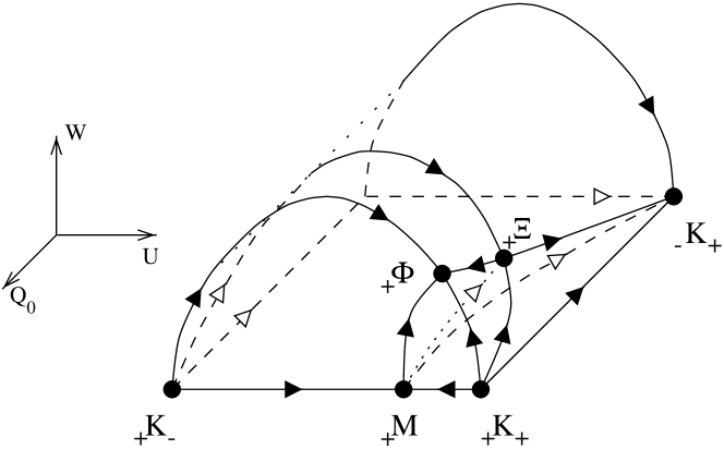
Figure 2: The state space for the $\Omega_{n}=0$, ${\bar{Q}_{+}}=-k{\bar{U}}$ submanifold for $k>1$ ($\kappa^{2}<2$). Dashed curves and white arrows are screened. The dotted curve between ${}_{+}{\rm M}$ and ${}_{+}\Xi$ is in the interior of the state space. The subscripts on the K-points refer to the sign of ${\bar{Q}_{0}}$ and ${\bar{U}}$, respectively. The state space is bounded by the following invariant submanifolds: the bottom is the massless scalar field submanifold (note that only part of the bottom is depicted – for a complete picture see Fig. 1d), the half-disks are plane-symmetric submanifolds, and the half-cylinder is the Kantowski-Sachs submanifold (${\bar{C}_{1}}=0$). Note that orbits and equilibrium points in the rear half have been suppressed for clarity.

9.2 Timelike self-similar case

In the TSS case, the reduced dynamical system becomes (eliminating the variable ${\tilde{C}_{1}}$):

$${\tilde{Q}_{0}}^{\prime} = -(1-{\tilde{Q}_{0}}^{2})\left[{\tilde{C}_{2}}^{2}-\frac{1+k^{2}}{k}({\tilde{Q}_{0}}-2k{\tilde{U}}){\tilde{U}}\right],$$ (87)

$${\tilde{U}}^{\prime} = -\frac{1}{k}\left(1-{\tilde{Q}_{0}}^{2}+2k{\tilde{Q}_{0}}{\tilde{U}}-\frac{2k^{2}}{1+k^{2}}\right)\left[1-(1+k^{2}){\tilde{U}}^{2}\right]$$ (88)

$$+\left({\tilde{Q}_{0}}{\tilde{U}}-\frac{2k}{1+k^{2}}\right){\tilde{C}_{2}}^{2},$$

$${\tilde{C}_{2}}^{\prime} = {\tilde{C}_{2}}\left[(1-{\tilde{Q}_{0}}^{2}+2k{\tilde{Q}_{0}}{\tilde{U}})\frac{1+k^{2}}{k}-{\tilde{Q}_{0}}(1-{\tilde{C}_{2}}^{2})\right].$$ (89)

The equilibrium points of this system are listed in table 6. They constitute a subset of the points listed in sections 6 and 7. In figures 3 and 4, some examples of state-space diagrams for this model are displayed.

Table 6: Equilibrium points in the $\Omega_{t}=0$, ${\tilde{Q}_{+}}=-k{\tilde{U}}$ submanifold. Note that subscripts on labels have been suppressed.

	${\tilde{Q}_{0}}$	${\tilde{U}}$	${\tilde{C}_{2}}$
C	${\epsilon}$	0	1
K	${\epsilon}$	$\pm\frac{1}{\sqrt{1+k^{2}}}$	0
M	${\epsilon}$	$\frac{k}{1+k^{2}}{\epsilon}$	0
X	${\epsilon}$	$\frac{1}{2k}{\epsilon}$	$\frac{1}{\sqrt{2}\,k}\sqrt{k^{2}-1}$	$k>1$ ($\kappa^{2}<2$)
$\Phi$	$\frac{2k}{\sqrt{1+k^{2}}}{\epsilon}$	$\frac{1}{\sqrt{1+k^{2}}}{\epsilon}$	0	$k^{2}<1/3$ ($\kappa^{2}>6$)
$Z$	$\sqrt{\frac{1-k^{2}}{1+k^{2}}}{\epsilon}$	0	0	$k<1$ ($\kappa^{2}>2$)

Figure 3: The state space for the $\Omega_{t}=0$, ${\tilde{Q}_{+}}=-k{\tilde{U}}$, ${\tilde{C}_{2}}=0$ submanifold for various values of $k$: (a) $k^{2}<1/3$ ($\kappa^{2}>6$); (b) $1/3<k^{2}<1$ ($2<\kappa^{2}<6$); (c) $k=1$ ($\kappa^{2}=2$) and (d) $k>1$ ($\kappa^{2}<2$). The subscripts on the K-points refer to the sign of ${\tilde{Q}_{0}}$ and ${\tilde{U}}$, respectively. Note the line bifurcation occurring for $k=1$ ($\kappa^{2}=2$).

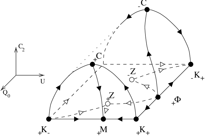
Figure 4: The state space for the $\Omega_{t}=0$, ${\tilde{Q}_{+}}=-k{\tilde{U}}$ submanifold for $k^{2}<1/3$ ($\kappa^{2}>6$). Dashed curves and white arrows and circles are screened. The subscripts on the K-points refer to the sign of ${\tilde{Q}_{0}}$ and ${\tilde{U}}$, respectively. The state space is bounded by the following invariant submanifolds: the bottom is the massless scalar field submanifold (note that only part of the bottom is depicted – for a complete picture see Fig. 3a), the half-disks are plane-symmetric submanifolds, and the half-cylinder is the static submanifold (${\tilde{C}_{1}}=0$). Note that orbits and equilibrium points in the rear half have been suppressed for clarity.

9.3 Discussion

In both the SSS and the TSS cases there are always attractors dominated by the kinetic part of the scalar field, corresponding to the K-equilibrium points. Consequently, there will always be solutions that expand from a K-singularity and recollapse to a K-singularity. When $\kappa^{2}>2$, the M-equilibrium points also are attractors. These correspond to dispersing solutions. Finally, there are $\Phi$-equilibrium points, which correspond to power-law inflationary solutions when $\kappa^{2}<2$. In the SSS case they act as attractors when $\kappa^{2}<2$, while in the TSS case they are attractors when $\kappa^{2}>6$.

To summarise, when $\kappa^{2}<2$ the SSS case contains recollapsing K $\rightarrow$ K solutions and power-law inflationary solutions K $\rightarrow$ $\Phi$. This is the same situation as for the Kantowski-Sachs models and closed Friedmann models examined in [29]. In contrast, when $\kappa^{2}<2$ the TSS case contains only recollapsing solutions. When $\kappa^{2}>2$, both the SSS and the TSS cases contain recollapsing solutions and also dispersing solutions K $\rightarrow$ M. The asymptotics is thus similar to the fluid-only case [23], where the generic regular solutions either are recollapsing K $\rightarrow$ K solutions or ever-expanding solutions K $\rightarrow$ M. Additionally, when $\kappa^{2}>6$ the TSS case also contains dispersing K $\rightarrow$ $\Phi$ solutions that are non-inflationary.

10 Massless scalar field

Critical phenomena in gravitational collapse were first found by Choptuik [36] in the study of a massless scalar field, and remain an active field of research (see, e.g., [37] and references therein). The solution at the threshold of black-hole formation in spherically symmetric radiation fluid collapse, corresponding to $\alpha=1/3$, was studied by Evans & Coleman [38]. In [35] a new class of ‘asymptotically Minkowski’ self-similar spacetimes were presented, which were shown to be intimately related to the so-called critical phenomena which arise in spherically symmetric gravitational collapse calculations [38].

Here, we present the governing equations for a self-similar massless scalar field in spherical symmetry. In this case, $\phi$ is still of the form

$$\phi=\Phi(\xi)+\sqrt{2}\,k\eta,$$ (90)

and the corresponding equations are formally obtained by setting $V=0$. In the presence of a barotropic fluid we then essentially have a non-interacting two-fluid model [20, 39], in which the massless scalar field can be identified with a stiff perfect fluid and the two fluids are separately conserved. We can then deduce that the models evolve from the massless scalar field model to the single-perfect fluid model [20, 39]. Hereafter, we shall assume that there is no barotropic fluid present, and that we are investigating a special case of the fluid vacuum model studied above. The massless scalar field equations without perfect fluid are then obtained by subsequently setting $\Omega_{n}=0$ and $\Omega_{t}=0$, respectively. This leads to the decoupling of $v$ and ${\bar{C}_{1}}$ in the SSS case, and $u$ and ${\tilde{C}_{1}}$ in the TSS case, respectively. Furthermore, in the SSS case ${\bar{W}}=0$, while in the TSS case, it follows that ${\tilde{Q}_{0}}={\epsilon}$ $(=\pm 1)$. The remaining dynamical systems are thus three-dimensional systems in $({\bar{Q}_{0}},{\bar{Q}_{+}},{\bar{U}})$ and $({\tilde{Q}_{+}},{\tilde{U}},{\tilde{C}_{2}})$, respectively. The constraint leads to two separate regions: either $C_{1}=0$ or else $Q_{+}=-kU$. Note that the latter is a special case of the models treated in section 9. Here, we briefly summarise the governing equations for these models and list all of the equilibrium points.

10.1 Spatially self-similar case

In the SSS case, the Friedmann equation becomes

$$0=1-{\bar{Q}_{+}}^{2}-(1+k^{2}){\bar{C}_{1}}^{2}-{\bar{U}}^{2},$$ (91)

which implies that

$$\bar{Z}\equiv 1-{\bar{Q}_{+}}^{2}-{\bar{U}}^{2}=(1+k^{2}){\bar{C}_{1}}^{2}.$$ (92)

The constraint becomes

$$0=({\bar{Q}_{+}}+k{\bar{U}})\bar{Z},$$ (93)

and the reduced dynamical system is

$${\bar{Q}_{0}}^{\prime} = -(1-{\bar{Q}_{0}}^{2})(1-2\bar{Z}),$$ (94)

$${\bar{Q}_{+}}^{\prime} = -2\bar{Z}\left({\bar{Q}_{0}}{\bar{Q}_{+}}+\frac{k^{2}}{1+k^{2}}\right),$$ (95)

$${\bar{U}}^{\prime} = -2\bar{Z}\left({\bar{Q}_{0}}{\bar{U}}-\frac{k}{1+k^{2}}\right).$$ (96)

The constraint implies that either $\bar{Z}$ or ${\bar{Q}_{+}}+k{\bar{U}}$ must be zero. When $\bar{Z}=0$, both ${\bar{Q}_{+}}$ and ${\bar{U}}$ are constants (subject to $1-{\bar{Q}_{+}}^{2}-{\bar{U}}^{2}=0$), whereby the dynamical system reduces to a single evolution equation for ${\bar{Q}_{0}}$, and consequently ${\bar{Q}_{0}}$ is monotonically decreasing. If the constant values of ${\bar{Q}_{+}}$ and ${\bar{U}}$ do not satisfy ${\bar{Q}_{+}}+k{\bar{U}}=0$, then the dynamics in the invariant set $\bar{Z}=0$ does not intersect with the dynamics in the invariant set ${\bar{Q}_{+}}+k{\bar{U}}=0$. The latter is contained within the fluid vacuum case studied in the previous section (see figure 1). The equilibrium points of the system are listed in table 7.

Table 7: Equilibrium points in the $\Omega_{n}=0$, ${\bar{W}}=0$ submanifold. Note that subscripts on labels have been suppressed.

	${\bar{Q}_{0}}$	${\bar{Q}_{+}}$	${\bar{U}}$
K-rings	${\epsilon}$,	${\bar{Q}_{+}}^{2}+{\bar{U}}^{2}=1$
M	${\epsilon}$,	$-k^{2}f{\epsilon}$	$kf{\epsilon}$	$f=1/(1+k^{2})$
X	$2kg{\epsilon}$	$-kg{\epsilon}$	$g{\epsilon}$	$g=1/(\sqrt{2}\sqrt{1+k^{2}})$

10.2 Timelike self-similar case

In the TSS case, the Friedmann equation becomes

$$0=1-{\tilde{Q}_{+}}^{2}-(1+k^{2}){\tilde{C}_{1}}^{2}-{\tilde{U}}^{2}-{\tilde{C}_{2}}^{2},$$ (97)

which implies that

$$\tilde{Z}\equiv 1-{\tilde{Q}_{+}}^{2}-{\tilde{U}}^{2}=(1+k^{2}){\tilde{C}_{1}}^{2}+{\tilde{C}_{2}}^{2}.$$ (98)

The constraint becomes

$$0=({\tilde{Q}_{+}}+k{\tilde{U}})({\tilde{C}_{2}}^{2}-\tilde{Z}),$$ (99)

and the reduced dynamical system is

$${\tilde{Q}_{+}}^{\prime} = -{\epsilon}{\tilde{Q}_{+}}(2\tilde{Z}-{\tilde{C}_{2}}^{2})+\frac{2k^{2}}{1+k^{2}}({\tilde{C}_{2}}^{2}-\tilde{Z}),$$ (100)

$${\tilde{U}}^{\prime} = -{\epsilon}{\tilde{U}}(2\tilde{Z}-{\tilde{C}_{2}}^{2})-\frac{2k}{1+k^{2}}({\tilde{C}_{2}}^{2}-\tilde{Z}),$$ (101)

$${\tilde{C}_{2}}^{\prime} = {\epsilon}{\tilde{C}_{2}}(1+{\tilde{C}_{2}}^{2}-2\tilde{Z}).$$ (102)

The constraint implies that either $\tilde{Z}={\tilde{C}_{2}}^{2}$ or ${\tilde{Q}_{+}}=-k{\tilde{U}}$. When $\tilde{Z}={\tilde{C}_{2}}^{2}$, the dynamical system becomes two-dimensional. The evolution equation for ${\tilde{C}_{2}}$ decouples and ${\tilde{C}_{2}}$ and ${\tilde{Q}_{+}}$ (or ${\tilde{U}}$) are monotonic. If the values of ${\tilde{Q}_{+}}$ and ${\tilde{U}}$ do not satisfy ${\tilde{Q}_{+}}+k{\tilde{U}}=0$, then the dynamics in the invariant set $\tilde{Z}={\tilde{C}_{2}}^{2}$ does not intersect with the dynamics in the invariant set ${\tilde{Q}_{+}}+k{\tilde{U}}=0$. The latter is contained within the fluid vacuum case studied in the previous section, and corresponds to the semi-disks at ${\tilde{Q}_{0}}=\pm 1$ in figure 4. The equilibrium points of the system are listed in table 8.

Table 8: Equilibrium points in the $\Omega_{t}=0$, ${\tilde{Q}_{0}}={\epsilon}$ submanifold. Note that subscripts on labels have been suppressed.

	${\tilde{Q}_{+}}$	${\tilde{U}}$	${\tilde{C}_{2}}$
C	0	0	1
K-ring	${\tilde{Q}_{+}}^{2}+{\tilde{U}}^{2}=1$		0
M	$-k^{2}f{\epsilon}$	$kf{\epsilon}$	0	$f=1/(1+k^{2})$
X	$-\frac{1}{2}{\epsilon}$	$\frac{1}{2k}{\epsilon}$	$\pm\frac{1}{\sqrt{2}\,k}\sqrt{k^{2}-1}$

10.3 Discussion

The dynamics is different in the various invariant submanifolds. The $\bar{Z}=0$ submanifold of the SSS case only contains recollapsing K $\rightarrow$ K solutions. The dynamics in the ${\bar{Q}_{+}}=-k{\bar{U}}$ submanifold of the SSS case is more complicated (see figure 1); when $\kappa^{2}<2$ there are only recollapsing K $\rightarrow$ K solutions, when $2<\kappa^{2}<6$ there are recollapsing solutions and dispersing K $\rightarrow$ M solutions, and when $\kappa^{2}>6$ there are also singularity-free bouncing M $\rightarrow$ M solutions, analogous to the bouncing Friedmann – Lemaître solutions. The TSS case only contains dispersing solutions. In the $\tilde{Z}={\tilde{C}_{2}}^{2}$ submanifold there are K $\rightarrow$ C solutions, while in the ${\tilde{Q}_{+}}=-{\tilde{U}}$ submanifold there are K $\rightarrow$ M solutions.

Appendix A Fluid quantities

For the non-tilted ($v=0$) equilibrium points of the SSS case, we have given the deceleration parameter $q_{\rm pf}$ with respect to the fluid congruence. The necessary expressions are summarised below.

The expansion of the fluid congruence is given by

$$\theta_{\rm pf} = \nabla_{a}u_{\rm pf}^{a}$$ (103)

$$= \frac{{\bar{Y}}e^{-x}}{\sqrt{3}\sqrt{1-v^{2}}}\left(\frac{vv^{\prime}}{1-v^{2}}+2{\bar{Q}_{0}}+{\bar{Q}_{+}}+3v{\bar{C}_{1}}\right),$$

and the deceleration parameter, defined by

$$q_{\rm pf} = -\left(1+3\frac{u_{\rm pf}^{a}\nabla_{a}\theta_{\rm pf}}{\theta_{\rm pf}^{2}}\right)$$ (104)

is given by

$$q_{\rm pf} = -1-\frac{3}{\left[\frac{vv^{\prime}}{1-v^{2}}+2{\bar{Q}_{0}}+{\bar{Q}_{+}}+3v{\bar{C}_{1}}\right]^{2}}\times$$ (105)

$$\left(2{\bar{Q}_{0}}^{\prime}+{\bar{Q}_{+}}^{\prime}+\frac{v(2{\bar{Q}_{0}}+{\bar{Q}_{+}})+{\bar{C}_{1}}(3-v^{2})}{1-v^{2}}v^{\prime}+\frac{1+2v^{2}}{(1-v^{2})^{2}}{v^{\prime}}^{2}\right.$$

$$+\frac{vv^{\prime\prime}}{1-v^{2}}-(2{\bar{Q}_{0}}+{\bar{Q}_{+}}+v^{\prime})\left\{{\bar{Q}_{+}}+{\bar{Q}_{0}}\left[2({\bar{Q}_{+}}^{2}+{\bar{U}}^{2})\right.\right.$$

$$\left.\left.+\frac{\gamma}{1+(\gamma-1)v^{2}}\Omega_{n}\right]\right\}-\left.\left\{2({\bar{Q}_{0}}-{\bar{Q}_{+}})+3v{\bar{C}_{1}}\right\}v{\bar{C}_{1}}\right).$$

Appendix B Transformation between the SSS and TSS variables

The two sets of variables basically differ only in the choice of dominant quantities (although one has to be careful, as the change of causality may result in sign change). Defining

$$\zeta = \frac{{\tilde{Y}}}{{\bar{Y}}}$$ (106)

$$= \sqrt{{\bar{Q}_{0}}^{2}-{\bar{W}}^{2}}$$ (107)

$$= \frac{1}{\sqrt{{\tilde{Q}_{0}}^{2}-{\tilde{C}_{2}}^{2}}},$$ (108)

the relations between the variable sets become

$${\bar{Q}_{0}}=\zeta{\tilde{Q}_{0}},\quad{\bar{Q}_{+}}=\zeta{\tilde{Q}_{+}},\quad{\bar{C}_{1}}=\zeta{\tilde{C}_{1}},\quad v=u^{-1},\quad U=\zeta{\tilde{U}},$$ (109)

$${\bar{W}}=\zeta\sqrt{{\tilde{Q}_{0}}^{2}-1},\quad{\tilde{C}_{2}}=\zeta^{-1}\sqrt{{\bar{Q}_{0}}^{2}-1}.$$ (110)

References

References

- [1] Guth A H 1981 Phys. Rev. D 23 347
- [2] Olive K A 1990 Phys. Rep. 190 307
- [3] Green M B, Schwarz J H and E. Witten 1987 Superstring Theory (Cambridge: Cambridge University Press)
- [4] Kaloper N, Madden R and Olive K A 1995 Nucl. Phys. B452 677
- [5] Halliwell J J 1987 Phys. Letts. B 185 341
- [6] Burd A B and Barrow J D 1988 Nucl. Phys. B308 929
- [7] Feinstein A and Ibáñez J 1993 Class. Quantum Grav. 10 93
- [8] Kitada Y and Maeda K 1992 Phys. Rev. D 45 1416
- [9] Kitada Y and Maeda K 1993 Class. Quantum Grav. 10 703
- [10] Coley A A, Ibáñez J and van den Hoogen R J 1997 J. Math. Phys 38 5256
- [11] van den Hoogen R J, Coley A A and Ibáñez J 1997 Phys. Rev. D. 55 1
- [12] van den Hoogen R J and Olasagasti I, preprint
- [13] Billyard A P, Coley A A, van den Hoogen R J, Ibáñez J and Olasagasti I 1999 Class. Quantum Grav. 16 4035
- [14] Copeland E J, Liddle A R and Wands D 1998 Phys. Rev. D 57 4686
- [15] Billyard A P, Coley A A and van den Hoogen R J 1998 Phys. Rev. D 58, 123501
- [16] van den Hoogen R J, Coley A A and Wands D 1999 Class. Quantum Grav. 16 1843
- [17] Coley A A, Ibáñez J and Olasagasti I 1998 Phys. Lett. A 250 75
- [18] Bogoyavlensky O I 1985 Methods in the qualitative theory of dynamical systems in astrophysics and gas dynamics (Berlin: Springer)
- [19] Carr B J and Coley A A 1999 Class. Quantum Grav. 16 R31
- [20] Carr B J and Coley A A 1999 A complete classification of spherically symmetric perfect fluid similarity solutions, preprint gr-qc/9901050
- [21] Goliath M, Nilsson U S and Uggla C 1998 Class. Quantum Grav. 15 167
- [22] Goliath M, Nilsson U S and Uggla C 1998 Class. Quantum Grav. 15 2841
- [23] Carr B J, Coley A A, Goliath M, Nilsson U S and Uggla C 1999, preprint gr-qc/9902070
- [24] Wainwright J 1996 in Proceedings of the forty sixth Scottish universities summer school in physics, Aberdeen ed G S Hall and J R Pulham (London: Institute of Physics publishing)
- [25] Cahill M E and Taub A H 1971 Commun. Math. Phys. 21 1
- [26] Wainwright J and Ellis G F R 1997 Dynamical Systems in Cosmology (Cambridge: Cambridge University Press)
- [27] Wetterich C 1988 Nucl. Phys. B302 668
- [28] Wetterich C 1995 Astron. Astrophys. 301 321
- [29] Coley A A and Goliath M 2000, preprint
- [30] Lin X-F and Wald R M 1989 Phys. Rev. D 40 3280
- [31] Lin X-F and Wald R M 1989 Phys. Rev. D 41 2444
- [32] Andersson L and Rendall A D 2000, preprint gr-qc/000104
- [33] Goliath M and Ellis G F R 1999 Phys. Rev. D 60 023502
- [34] Goliath M and Nilsson U S 2000 Isotropization of two-component fluids, preprint
- [35] Carr B J, Coley A A, Goliath M, Nilsson U S and Uggla C 2000 Phys. Rev. D 61 081502(R)
- [36] Choptuik M W 1993 Phys. Rev. Lett. 70 9
- [37] Gundlach C 1999 Living Reviews 2 1999-4, available at http://www.livingreviews.org/
- [38] Evans C R and Coleman J S 1994 Phys. Rev. Lett. 72 1782
- [39] Coley A A and Wainwright J 1992 Class. Quantum Grav. 9 651