Boost-rotation symmetric spacetimes – review

Abstract

Boost-rotation symmetric spacetimes are the only locally asymptotically flat axially symmetric electrovacuum spacetimes with a further symmetry that are radiative. They are realized by uniformly accelerated particles of various kinds or black holes. Their general properties are summarized. Several examples of boost-rotation symmetric solutions of the Maxwell and Einstein equations are studied: uniformly accelerated electric and magnetic multipoles, the Bonnor-Swaminarayan solutions, the C-metric and the spinning C-metric.

Contents

toc

I Introduction

There exists only one class of exact radiative solutions of the full nonlinear Einstein equations which are known in an analytical form, realized by moving objects and, in addition, are asymptotically flat (in some cases null infinity ${\cal J}$ is even global [2]). This is the class of boost-rotation symmetric spacetimes describing uniformly accelerated particles or black holes symmetrically located along the symmetry axis (see reviews [3, 4, 5]). They have two Killing vectors, the axial Killing vector with circular group orbits and the boost Killing vector which asymptotically goes over to the generator of the Lorentz transformation along the symmetry axis in the Minkowski spacetime. The significance of these solutions follows from the theorem which states that among locally asymptotically flat spacetimes with the axial and an additional symmetry, boost-rotation symmetric spacetimes are the only spacetimes which are radiative. It was proved in [6] for vacuum spacetimes with hypersurface orthogonal Killing vectors and generalized in [7] for electrovacuum spacetimes with Killing vectors which are not hypersurface orthogonal. These spacetimes have been found also useful in numerical relativity as test beds for numerical codes (approaches based on null [8, 9] and spacelike [10] initial hypersurfaces).

Several boost-rotation symmetric solutions are known. The first boost-rotation symmetric solution, that has been found, is the C-metric [11, 12], describing accelerated black holes symmetrically located on the axis of symmetry with a nodal (conical) singularity (“cosmic string”) which causes the acceleration. Another example is a set of Bonnor-Swaminarayan solutions [13] representing a finite number of uniformly accelerated monopole “Curzon-Chazy” particles. The acceleration can be caused by nodal singularities or by mutual gravitational interaction. However, in the case with no nodal singularities, negative masses occur. The simplest case without conical singularity is represented by two pairs of particles, in each of which there is one particle with positive and one with negative mass (as an analogous system in the Newton mechanics, such a system is self-accelerated). A limiting procedure (similar to that in electromagnetism by which one obtains a dipole from two monopoles) leads to a special solution [14] realized by two independent, self-accelerating particles. Such a solution is asymptotically flat, admitting global null infinity ${\cal J}$. Boost-rotation symmetric solutions with a cosmic string extending along the whole axis of symmetry are locally asymptotically flat in the sense that they admit only local ${\cal J}$. Boost-rotation symmetric solutions describing uniformly accelerated particles with a general multipole structure were also found in [14]. There exist generalizations of the vacuum boost-rotation symmetric spacetimes containing an electromagnetic field – the charged C-metric [15], or rotating sources – the spinning C-metric [16, 17]. The Killing vectors in the case of a spinning source are not hypersurface orthogonal. Also the generalized C-metric [18], generalized charged C-metric [19], and generalized Bonnor-Swaminarayan solution [14] are known that are not asymptotically flat and in which an external field is present to cause the acceleration.

Section II is devoted to the general theory of boost-rotation symmetric spacetimes. It is divided into two parts. In the first part II A we recall the Bondi method we further use to present the theorem about uniqueness of boost-rotation symmetric spacetimes among all locally asymptotically flat electrovacuum axially symmetric spacetimes with an additional symmetry. In the second part II B, based on [20], the definition and general features of boost-rotation symmetric spacetimes are summarized.

Sec. III discusses several examples of boost-rotation symmetric solutions: uniformly accelerated electric and magnetic multipoles, the Bonnor-Swaminarayan solutions, the C-metric and the spinning C-metric.

We use the signature $-2$ everywhere except for the last two parts concerning the standard and spinning C-metrics where the signature $+2$ is used following [16, 17].

II Theoretical background

A Asymptotically flat axisymmetric spacetimes and radiation

1 The Bondi method

If one is interested in gravitational radiation from a general bounded matter source, i.e., in the behaviour of gravitational field far from the source, one has to turn to approximation methods, typically one expands the metric in negative powers of a suitably chosen “radial coordinate” $r$. This was done for axially symmetric non-rotating sources by Bondi et al. [21] (generalized without this assumption by Sachs [22], for charged sources by van der Burg [23] – mistakes were corrected in [7], for spacetimes with null dust by von der Gönna and Kramer [24] and for spacetimes with polyhomogeneous ${\cal J}$ by Chruściel et al. [25]). They introduced suitably chosen coordinates $\{u,\ r,\ \theta,\ \phi\}$ in such a way that, roughly speaking, null coordinate $u$, spherical angles $\theta$ and $\phi$ are constant along outgoing radial null geodesics – light rays – meanwhile $r$, the luminosity distance, varies and satisfies the condition $g_{\theta\theta}g_{\phi\phi}=r^{4}\sin^{2}\theta$ so that the area of the surface $u=$ const, $r=$ const, $\phi\in\langle 0,2\pi)$, and $\theta\in\langle 0,\pi\rangle$ is $4\pi r^{2}$.

The Bondi method meant a breakthrough in gravitational radiation theory. It consists in prescribing initial data not on a spacelike Cauchy hypersurface and solving the Cauchy problem (which is well posed for the Einstein equations [26]) but in prescribing initial data on a characteristic hypersurface of the quasilinear hyperbolic Einstein equations which is null, i.e., on a hypersurface $u=$ const. Then discontinuities can arise and the Cauchy problem is ambiguous. One has to prescribe initial data not only on the initial null hypersurface but one also has to know two functions, $c,_{u}$ and $d,_{u}$ (in the vacuum case), for all $u$ (or $u$ in the given interval). Only then the evolution of the gravitational field is known, i.e., determined for all $u$ (or in the given interval). This is why we call these two functions the news functions of the system because they carry the whole information about changes in the system. If and only if one of them does not vanish the total mass of the system as measured at null infinity, the Bondi mass, decreases and gravitational waves are radiated. If the $u$-derivative of at least one of the news functions does not vanish the Weyl tensor has radiative tetrad components (proportional to $r^{-1}$)

$$C_{\alpha\beta\gamma\delta}m^{\alpha}t^{\beta}m^{\gamma}t^{\delta}=[(c+{\rm i}d)_{,uu}]\frac{1}{r}+{\cal O}(r^{-2})\$$ (1)

in the standard null tetrad $\{k^{\alpha},\ m^{\alpha},\ t^{\alpha},\ {\bar{t}}^{\alpha}\}$ introduced in [22, 7]. There are exceptional cases corresponding, e.g., to an infinite string (thus the axis of axial symmetry is not regular) with a non-zero news function and with a non-radiative Weyl tensor [27].

Hereafter we are interested in asymptotically flat electrovacuum spacetimes that are in addition axially symmetric but a source can rotate and we thus follow the work of van der Burg [23] with the additional assumption that all metric functions do not depend on $\phi$. The metric has, in the Bondi-Sachs coordinates { $u$, $r$, $\theta$, $\phi$ } $\equiv$ { $x^{0}$, $x^{1}$, $x^{2}$, $x^{3}$}, the form

$${\rm d}s^{2} = \left(\frac{V}{r}{\rm e}^{2\beta}-r^{2}{\rm e}^{2\gamma}U^{2}\cosh 2\delta-r^{2}{\rm e}^{-2\gamma}W^{2}\cosh 2\delta-2r^{2}UW\sinh 2\delta\right){\rm d}u^{2}$$ (5)

$$\ +2{\rm e}^{2\beta}{\rm d}u{\rm d}r+2r^{2}\left({\rm e}^{2\gamma}U\cosh 2\delta+W\sinh 2\delta\right){\rm d}u{\rm d}\theta$$

$$\ +2r^{2}\left({\rm e}^{-2\gamma}W\cosh 2\delta+U\sinh 2\delta\right)\sin\theta\ {\rm d}u{\rm d}\phi$$

$$\ -r^{2}\left[\cosh 2\delta\left({\rm e}^{2\gamma}{\rm d}\theta^{2}+{\rm e}^{-2\gamma}\sin^{2}\theta\ {\rm d}\phi^{2}\right)+2\sinh 2\delta\sin\theta\ {\rm d}\theta{\rm d}\phi\right]\ ,$$

where all the six metric functions $U$, $V$, $W$, $\beta$, $\gamma$, $\delta$ and the electromagnetic field $F_{\mu\nu}$ do not depend on $\phi$ because of the axial symmetry. If one requires the axis of the axial symmetry ($\theta=0$, $\pi$) to be regular, then functions

$$V,\mbox{\quad}\beta,\mbox{\quad}W,\mbox{\quad}\gamma/\sin^{2}\theta,\mbox{\quad}U/\sin\theta,\mbox{\quad}\delta/\sin\theta$$ (6)

have to be regular for $\sin\theta\rightarrow 0$.

First assuming the functions $\gamma$, $\delta$, $F_{12}$ and $F_{13}$ to have asymptotic expansions, the spacetime to be asymptotically flat, and only the outgoing radiation to be asymptotically present then the expansions of these four functions at large $r$ on an initial hypersurface $u=$ const are of the form

$$\gamma = \frac{c}{r}+(C-{{\scriptstyle{\frac{1}{6}}}}c^{3}-{{\scriptstyle{\frac{3}{2}}}}cd^{2})\frac{1}{r^{3}}+\frac{D}{r^{4}}+{\cal O}(r^{-5})\ ,$$ (7)

$$\delta = \frac{d}{r}+(H-{{\scriptstyle{\frac{1}{6}}}}d^{3}+{{\scriptstyle{\frac{1}{2}}}}c^{2}d)\frac{1}{r^{3}}+\frac{K}{r^{4}}+{\cal O}(r^{-5})\ ,$$ (8)

$$F_{12} = \frac{e}{r^{2}}+(2E+ec+fd)\frac{1}{r^{3}}+{\cal O}(r^{-4})\ ,$$ (9)

$$F_{13} = \biggl{[}\frac{f}{r^{2}}+(2F+ed-fc)\frac{1}{r^{3}}+{\cal O}(r^{-4})\biggr{]}\sin\theta\ .$$ (10)

Prescribing then initial data on this null hypersurface, i.e., $c$, $d$, $C$, … and $M$, $N$, $P$, $\epsilon$, $\mu$ as functions of $\theta$, all the other metric functions are determined on the initial hypersurface by the field equations:

$$\beta = -{{\scriptstyle{\frac{1}{4}}}}(c^{2}+d^{2})\frac{1}{r^{2}}+{\cal O}(r^{-4})\ ,$$ (11)

$$U = -(c,_{\theta}+2c\cot\theta)\frac{1}{r^{2}}+\Bigl{[}2N+3(cc,_{\theta}+dd,_{\theta})+4(c^{2}+d^{2})\cot\theta\Bigr{]}\frac{1}{r^{3}}$$ (13)

$$+{{\scriptstyle{\frac{1}{2}}}}\Bigl{[}3(C,_{\theta}+2C\cot\theta)-6(cN+dP)-4(2c^{2}c,_{\theta}+cdd,_{\theta}+c,_{\theta}d^{2})-8c(c^{2}+d^{2})\cot\theta+2(\epsilon e-f\mu)\Bigr{]}\frac{1}{r^{4}}+{\cal O}(r^{-5})\ ,$$

$$W = -(d,_{\theta}+2d\cot\theta)\frac{1}{r^{2}}+\Bigl{[}2P+2(c,_{\theta}d-cd,_{\theta})\Bigr{]}\frac{1}{r^{3}}$$ (15)

$$+{{\scriptstyle{\frac{1}{2}}}}\Bigl{[}3(H,_{\theta}+2H\cot\theta)+6(cP-dN)-4(2d^{2}d,_{\theta}+cdc,_{\theta}+c^{2}d,_{\theta})-8d(c^{2}+d^{2})\cot\theta+2(\mu e+\epsilon f)\Bigr{]}\frac{1}{r^{4}}+{\cal O}(r^{-5})\ ,$$

$$V = r-2M-\Bigl{[}N,_{\theta}+N\cot\theta-{{\scriptstyle{\frac{1}{2}}}}(c^{2}+d^{2})-(c,_{\theta}+2c\cot\theta)^{2}-(d,_{\theta}+2d\cot\theta)^{2}-(\epsilon^{2}+\mu^{2})\Bigr{]}\frac{1}{r}$$ (18)

$$-{{\scriptstyle{\frac{1}{2}}}}\Bigl{[}C,_{\theta\theta}+3C,_{\theta}\cot\theta-2C+6N(c,_{\theta}+2c\cot\theta)+6P(d,_{\theta}+2d\cot\theta)+4(2cc,_{\theta}^{2}+3c,_{\theta}dd,_{\theta}-cd,_{\theta}^{2})$$

$$+8(2c,_{\theta}d^{2}+3c^{2}c,_{\theta}+cdd,_{\theta})\cot\theta+16c(c^{2}+d^{2})\cot^{2}\theta+2\epsilon(e,_{\theta}+e\cot\theta)-2\mu(f,_{\theta}+f\cot\theta)\Bigr{]}\frac{1}{r^{2}}+{\cal O}(r^{-3})\ ,$$

$$F_{01} = -\frac{\epsilon}{r^{2}}+(e,_{\theta}+e\cot\theta)\frac{1}{r^{3}}+{\cal O}(r^{-4})\ ,$$ (19)

$$F_{23} = \Bigl{[}-\mu-(f,_{\theta}+f\cot\theta)\frac{1}{r}+{\cal O}(r^{-2})\Bigr{]}\sin\theta\ ,$$ (20)

$$F_{02} = X+(\epsilon,_{\theta}-e,_{u})\frac{1}{r}-\Bigr{\{}[E+{{\scriptstyle{\frac{1}{2}}}}(ec+fd)],_{u}+{{\scriptstyle{\frac{1}{2}}}}(e,_{\theta}+e\cot\theta),_{\theta}\Bigl{\}}\frac{1}{r^{2}}+{\cal O}(r^{-3})\ ,$$ (21)

$$F_{03} = \Biggl{\{}Y-\frac{f,_{u}}{r}-\Bigl{[}[F+{{\scriptstyle{\frac{1}{2}}}}(ed-fc)],_{u}\Bigr{]}\frac{1}{r^{2}}+{\cal O}(r^{-3})\Biggr{\}}\sin\theta\ .$$ (22)

Provided four news functions, two gravitational, $c,_{u}$, $d,_{u}$, and two electromagnetic, $X$, $Y$, are prescribed for all $u$, the time evolution of the system is fully determined using the Einstein-Maxwell equations (see [23] for details). Let us just mention a relation for the mass aspect $M$ which is equal in stationary case to the total mass of the system:

$$M,_{u}=-(c,_{u}^{2}+d,_{u}^{2})-(X^{2}+Y^{2})+{{\scriptstyle{\frac{1}{2}}}}(c,_{\theta\theta}+3c,_{\theta}\cot\theta-2c),_{u}\ .$$ (23)

Then the total mass at future null infinity ${\cal J}^{+}$ at a given “retarded time” $u$, the Bondi mass $m$, defined as a mean value of the mass aspect of the system, $M$, over the sphere,

$$m(u)={{\scriptstyle{\frac{1}{2}}}}\int_{0}^{\pi}M(u,\theta)\sin\theta{\rm d}\theta\ ,$$ (24)

is decreasing if at least one of the news functions does not vanish:

$$m,_{u}=-{{\scriptstyle{\frac{1}{2}}}}\int\limits_{0}^{\pi}(c,_{u}^{2}+d,_{u}^{2}+X^{2}+Y^{2})\sin\theta{\rm d}\theta\leq 0\ .$$ (25)

The mass decrease is caused by gravitational and electromagnetic waves radiated out from the system.

The rate of loss of the electromagnetic energy radiated out from the system is given by

$$\frac{\partial}{\partial u}\int\limits_{0}^{\pi}{{\scriptstyle{\frac{1}{2}}}}(X^{2}+Y^{2})\sin\theta{\rm d}\theta\ ,$$ (26)

which indeed implies the loss of mass as seen from Eq. (25).

There are several conserved quantities described in [23, 28]. Two of them are the electric and magnetic charges of the source

$$\frac{\partial}{\partial u}\int\limits_{0}^{\pi}{{\scriptstyle{\frac{1}{2}}}}\epsilon\sin\theta{\rm d}\theta=0\ ,\mbox{\quad}\mbox{\quad}\frac{\partial}{\partial u}\int\limits_{0}^{\pi}{{\scriptstyle{\frac{1}{2}}}}\mu\sin\theta{\rm d}\theta=0\ .$$ (27)

2 Symmetries of asymptotically flat axisymmetric electrovacuum spacetimes and radiation

Since finding an exact radiative solution describing a general charged bounded source is a very difficult task, may be unsolvable, it is of interest to know which isometries are compatible with asymptotic flatness and admit radiation. This question was solved in [6] for locally asymptotically flat axially symmetric vacuum spacetimes with non-rotating sources, i.e., with hypersurface orthogonal Killing vectors, and generalized in [7] for electrovacuum spacetimes with, in general, rotating sources, i.e., with Killing vectors that are not hypersurface orthogonal. The assumption of axial symmetry with the corresponding Killing vector field denoted by $\xi=\partial/\partial\phi$ simplifies lengthy calculations.

Suppose that such an axially symmetric electrovacuum spacetime admits only a “piece” of future null infinity ${\cal J}^{+}$ in the sense of [2]. Then one can introduce the Bondi-Sachs coordinate system { $u$, $r$, $\theta$, $\phi$ } $\equiv$ { $x^{0}$, $x^{1}$, $x^{2}$, $x^{3}$} in which the metric has the form (5), where the metric functions and the electromagnetic field $F_{\mu\nu}$ are functions of $u$, $r$, $\theta$ and have expansions (8), (19). Thanks to the existence of only local ${\cal J}^{+}$, we assume Eqs. (8)–(23) to be satisfied for all $\phi\in\langle 0,2\pi)$, however, not necessarily on the whole sphere, i.e., not for all $\theta\in\langle 0,\pi\rangle$ but only in some open interval of $\theta$ and thus the Bondi mass (24) cannot be introduced. For example, the “axis of symmetry” ($\theta=0$, $\pi$) may contain nodal singularities and thus need not be regular and the regularity conditions on the axis (6) need not be satisfied for any $u$. If the axis is singular then at least two generators of ${\cal J}^{+}$ would be missing so that ${\cal J}^{+}$ would not be topologically $S^{2}\times{\cal R}$.

Let us now assume that another Killing vector field $\eta$ exists which forms together with $\xi=\partial/\partial\phi$ a two-parameter group. In Ref. [6] it is proved (see Lemma in Sec. 2) that in the case of $\xi$ with circles as integral curves, $\xi$ and $\eta$ determine an Abelian Lie algebra so that we can assume $[\eta,\xi]=0$. Hence, the components $\eta^{\alpha}$ are independent of $\phi$.

Then by solving the Killing equations ${\cal L}_{\eta}g_{\alpha\beta}=0$ (explicitly given in [7, 29]), the Killing vector asymptotically turns out to be

$$\eta^{\alpha}=[-ku\cos\theta+\alpha(\theta),\ kr\cos\theta+{\cal O}(r^{0}),\ -k\sin\theta+{\cal O}(r^{-1}),\ {\cal O}(r^{-1})]\ ,$$ (28)

where $k$ is a constant and $\alpha$ an arbitrary function of $\theta$. This result for a locally asymptotically flat axially symmetric electrovacuum spacetime with Killing vectors which need not be hypersurface orthogonal proved in [7] is the same as that one for asymptotically flat axially symmetric vacuum spacetimes with hypersurface orthogonal Killing vectors obtained in [6].

Let us analyze possibilities $k=0$ and $k\not=0$ separately.
1) Case $k=0$
This alternative was considered in [7] and developed in detail in [30]. When $k=0$, the Killing vector field $\eta$ (28) generates supertranslations. However, solving Killing equations in higher orders of $r^{-1}$ and assuming that the electromagnetic field described by $F_{\mu\nu}$ (8), (19) has the same symmetry, i.e., ${\cal L}_{\eta}F_{\alpha\beta}=0$, one can show that $\eta$ in fact generates translations

$$\eta^{\alpha} = \Bigl{[}B,\ Bc,_{u}+B,_{\theta}\cot\theta-\frac{uc,_{u}^{2}B}{r}+{\cal O}(r^{-2}),\ -B,_{\theta}\frac{1}{r}+B,_{\theta}\frac{c}{r^{2}}+{\cal O}(r^{-3}),\ {\cal O}(r^{-4})\Bigr{]}\ ,$$ (29)

where

$$B(\theta)=\frac{\sin\theta}{2{\rm C}}\biggl{[}(b_{0}+a_{0})\Bigl{(}\frac{\sin\theta}{\cos\theta+1}\Bigr{)}^{\rm C}+(b_{0}-a_{0})\Bigl{(}\frac{\sin\theta}{\cos\theta+1}\Bigr{)}^{-\rm C}\biggr{]}\ ,$$ (30)

with constants $a_{0}$, $b_{0}$ and ${\rm C}\in(0,1\rangle$ in a spacetime with, in general, an infinite thin cosmic string along the symmetry axis. The cosmic string is described by a deficit angle $2\pi(1-{\rm C})$. The only non-vanishing news function – due to the presence of the string – is

$$c,_{u}=\frac{{\rm C}^{2}-1}{2\sin^{2}\theta}\ ,$$ (31)

which depends only on $\theta$ and thus the Weyl tensor (1) does not have a radiative character. The leading metric functions and electromagnetic field functions have the form

$$c(u,\ \theta) = \frac{u}{2B}(B,_{\theta\theta}-B,_{\theta}\cot\theta)=u\frac{{\rm C}^{2}-1}{2\sin^{2}\theta}\ ,\mbox{\quad}d(u,\ \theta)=0\ ,$$ (32)

$$M(u,\ \theta) = -uc,_{u}^{2}-a_{1}B^{-3}\ ,$$ (33)

$$N(u,\ \theta) = -{{\scriptstyle{\frac{1}{2}}}}B^{-4}(2a_{1}B,_{\theta}u+f_{0}\sin\theta)\ ,\mbox{\quad}P(u,\ \theta)=-{{\scriptstyle{\frac{1}{2}}}}g_{0}\sin\theta B^{-4}\ ,$$ (34)

$$X(u,\ \theta) = Y(u,\ \theta)=0\ ,\mbox{\quad}\epsilon(u,\ \theta)=\epsilon_{0}B^{-2}\ ,\mbox{\quad}\mu(u,\ \theta)=\mu_{0}B^{-2}\ ,$$ (35)

$$e(u,\ \theta) = -\epsilon_{0}B,_{\theta}B^{-3}u+e_{1}(\theta)\ ,\mbox{\quad}f(u,\ \theta)=\mu_{0}B,_{\theta}B^{-3}u+f_{1}(\theta)\ ,$$ (36)

where $a_{1}$, $f_{0}$, $g_{0}$, $\epsilon_{0}$, and $\mu_{0}$ are constants and $e_{1}$, $f_{1}$ are arbitrary functions of $\theta$. The reader may find more metric and field functions in [29] and [30].

In paper [30] we proved the following statements in Theorems 1, 2. The asymptotically translational Killing vector $\eta$, given by (29), has asymptotically the norm

$$\|\eta\|^{2} = (b_{0}^{2}-a_{0}^{2})+\frac{2a_{1}}{B}\frac{1}{r}+[u2a_{1}B^{-3}(B^{2}c,_{u}-B,_{\theta}^{2}+BB,_{\theta}\cot\theta)$$ (38)

$$\mbox{\quad}+f_{0}\sin\theta\ B^{-3}(-B,_{\theta}+B\cot\theta)+(\epsilon_{0}^{2}+\mu_{0}^{2})B^{-2}]\frac{1}{r^{2}}+{\cal O}(r^{-3})\ ,$$

that may be spacelike, timelike or null. It is spacelike for $a_{0}^{2}>b_{0}^{2}$. If one of the constants $a_{1}$, $f_{0}$ or $g_{0}$ is non-vanishing then ${\cal J}^{+}$ is singular at $\theta=\theta_{0}\not=0$, $\pi$, given by the relation

$$\cos\theta_{0}=\frac{(a_{0}+b_{0})^{2/{\rm C}}-(a_{0}^{2}-b_{0}^{2})^{1/{\rm C}}}{(a_{0}+b_{0})^{2/{\rm C}}+(a_{0}^{2}-b_{0}^{2})^{1/{\rm C}}}\ ,$$ (39)

in addition to the singularity due to the presence of the cosmic string at $\theta=0$, $\pi$. This case corresponds to cylindrical waves (in particular, $\theta_{0}=\pi/2$ for $b_{0}=0$). The Killing vector $\eta$ is null if $a_{0}=\pm b_{0}$. Then ${\cal J}^{+}$ is singular at $\theta=0$ or $\pi$ in addition to the string singularity if again $a_{1}$ or $f_{0}$ or $g_{0}$ is non-vanishing. It corresponds to a wave propagating along the symmetry axis. The Killing vector $\eta$ is timelike for $a_{0}^{2}<b_{0}^{2}$ and the only singularities of ${\cal J}^{+}$ at $\theta=0$, $\pi$ are due to the presence of the string.

If there is no string, null infinity ${\cal J}^{+}$ may be regular even with a non-vanishing Bondi mass $m$ for an asymptotically timelike translational Killing vector. However, even if the translational Killing vector is spacelike or null, ${\cal J}^{+}$ may be regular if the spacetime is flat in its neighbourhood (i.e., constants $a_{1}$, $f_{0}$, $g_{0}$ and thus also the mass aspect $M$ and functions $N$, $P$, … vanish).

For $\rm C=1$, without the string, we find the Killing vector field $\eta$ (29) to have asymptotically the form

$$\eta^{\alpha}=\Bigl{[}-a_{0}\cos\theta+b_{0},\ a_{0}\cos\theta+{\cal O}(r^{-2}),\ -\frac{a_{0}\sin\theta}{r}+{\cal O}(r^{-4}),\ {\cal O}(r^{-4})\Bigr{]}$$ (40)

and the mass aspect is then given by

$$M=-\frac{a_{1}}{(-a_{0}\cos\theta+b_{0})^{3}}\ .$$ (41)

In the case of the timelike Killing vector ($b_{0}^{2}>a_{0}^{2}$) assuming $b_{0}>0$ and $a_{1}<0$ we obtain the total Bondi mass to be

$$m=-\frac{a_{1}b_{0}}{(b_{0}^{2}-a_{0}^{2})^{2}}>0\ .$$ (42)

The factor $-a_{0}\cos\theta+b_{0}$ appearing in Eq. (41) corresponds, using the terminology of [21], to the “Doppler shift of the mass aspect” and the other Bondi functions. It occurs when the system is boosted with respect to the Bondi frame with the boost parameter – $\nu$ ($b_{0}=\cosh\nu$, $a_{0}=\sinh\nu$) so that its velocity is $v=-\tanh\nu=a_{0}/b_{0}$. Putting $a_{1}=-{\bar{m}}$, we get the mass aspect in Eq. (41) in the form $M={\bar{m}}/(\cosh\nu-\sinh\nu\cos\theta)^{3}$, which exactly corresponds to the formula (see Eq. (72) in [21]) for the Schwarzschild mass ${\bar{m}}$ moving along the axis of symmetry with constant velocity $-\tanh\nu$.

In [30] two exact solutions are studied with axial and translational Killing vectors and with an infinite cosmic string along the symmetry axis – the Schwarzschild solution with a string, where the Killing vector generates translations along the $t$-axis ($a_{1}\not=0$, $f_{0}=g_{0}=0$) and Einstein-Rosen cylindrical waves with a string having a spacelike translational Killing vector corresponding to translations along the $z$-axis ($a_{1}=0$, $f_{0}\not=0$, $g_{0}=0$).
2) Case $k\not=0$
Assuming $k\not=0$ in (28), it is easy to find a Bondi-Sachs coordinate system with $\alpha=0$ by performing a supertranslation. Hence we put $\alpha=0$ in (28) and without loss of generality we choose $k=1$. Then the asymptotic form of the Killing vector field $\eta$ is

$$\eta^{\alpha}=[-u\cos\theta,\ r\cos\theta+{\cal O}(r^{0}),\ -\sin\theta+{\cal O}(r^{-1}),\ {\cal O}(r^{-1})]\ .$$ (43)

It is the boost Killing vector that generates the Lorentz transformation along the axis of axial symmetry.

Solving the Killing equations in higher orders of $r^{-1}$ and assuming that the electromagnetic field has the same symmetry, i.e., ${\cal L}_{\eta}F_{\mu\nu}=0$ is satisfied, we obtain the forms of the metric and field functions to be:

$$c(u,\theta) = -\frac{{\cal K}(w)}{uw}\mbox{\quad}\rightarrow\ c,_{u}=\frac{{\cal K}(w),_{w}}{u^{2}}\ ,$$ (44)

$$d(u,\theta) = -\frac{{\cal L}(w)}{uw}\mbox{\quad}\rightarrow\ d,_{u}=\frac{{\cal L}(w),_{w}}{u^{2}}\ ,$$ (45)

$$M(u,\theta) = \frac{1}{2\sin\theta}(w^{2}{\cal K},_{w}),_{w}+\frac{\lambda(w)}{u^{3}w^{3}}\ ,$$ (46)

$$X(u,\theta) = \frac{{\cal E}(w)}{u^{2}}\ ,$$ (47)

$$Y(u,\theta) = \frac{{\cal B}(w)}{u\sin\theta}=\frac{{\cal B}(w)}{wu^{2}}=\frac{\tilde{{\cal B}}(w)}{u^{2}}\ ,$$ (48)

$$\epsilon(u,\theta) = \frac{{\cal E}(w)}{u}\cot\theta\ ,$$ (49)

$$\mu(u,\theta) = \frac{{\cal B}(w)}{\sin\theta}\cot\theta=\frac{\tilde{{\cal B}}(w)}{u}\cot\theta\ ,$$ (50)

$$e(u,\theta) = \frac{{\cal E}(w)}{2}+\frac{{\cal G}(w)}{u^{2}}\ ,$$ (51)

$$f(u,\theta) = -\frac{{\cal B}(w)u}{2\sin\theta}+\frac{{\cal D}(w)}{u\sin\theta}=-\frac{\tilde{{\cal B}}(w)}{2}+\frac{\tilde{{\cal D}}(w)}{u^{2}}\ ,$$ (52)

where $w=\sin\theta/u$, functions ${\cal K}(w)$, ${\cal L}(w)$, ${\cal E}(w)$ and ${\cal B}(w)$ ($\tilde{{\cal B}}(w)={\cal B}(w)/w$) are arbitrary functions determining news functions, and $\lambda(w)$ has to satisfy the equation

$$\lambda,_{w}=w^{2}({\cal K},_{w}^{2}+{\cal L},_{w}^{2}+{\cal E}^{2}+\tilde{{\cal B}}^{2})-\frac{1}{2w}(w^{3}{\cal K},_{ww}),_{w}\ ,$$ (53)

while ${\cal G}(w)$ and ${\cal D}(w)$ ($\tilde{{\cal D}}(w)={\cal D}(w)/w$) are solutions of the equations

$$2w^{2}({\cal G},_{w}w+2{\cal G})+({\cal E},_{w}w-{\cal E})+2w{\cal E}{\cal K}+2{\cal B}{\cal L}\hskip 17.07164pt = 0\ ,$$ (54)

$$2w^{2}({\cal D},_{w}w+{\cal D})-({\cal B},_{w}w-2{\cal B})-2w{\cal B}{\cal K}+2w^{2}{\cal E}{\cal L} = 0\ .$$ (55)

Solving Eq. (53) for $\lambda$ with prescribed news functions (i.e., for given ${\cal K}(w),_{w}$, ${\cal L}(w),_{w}$, ${\cal E}(w)$ and $\tilde{{\cal B}}(w)$) we find the mass aspect $M(u,\ \theta)$ (46) and thus the total Bondi mass at ${\cal J}^{+}$ is then given by

$$m(u)={{\scriptstyle{\frac{1}{2}}}}\int\limits_{0}^{\pi}M(u,\theta)\sin\theta\ {\rm d}\theta\ ={{\scriptstyle{\frac{1}{4}}}}\int\limits_{0}^{\pi}(w^{2}{\cal K},_{w}),_{w}{\rm d}\theta+{{\scriptstyle{\frac{1}{2}}}}\int\limits_{0}^{\pi}\frac{\lambda}{u^{2}w^{2}}\ {\rm d}\theta\ .$$ (56)

The expansion of the boost Killing vector is as follows

$$\eta^{\alpha} = \Bigl{[}-u\cos\theta\ ,\ r\cos\theta+u\cos\theta+\cos\theta\ \Bigl{(}{\cal K},_{w}+\frac{{\cal K}}{w}\Bigr{)}\ \frac{1}{r}+{\cal O}(r^{-2})\ ,\$$ (58)

$$\ -\sin\theta-\frac{u\sin\theta}{r}+\frac{uc\sin\theta}{r^{2}}+{\cal O}(r^{-3})\ ,\ \frac{ud}{r^{2}}+{\cal O}(r^{-3})\Bigr{]}\ .$$

These results were generalized for spacetimes with in general polyhomogeneous ${\cal J}$ using Newman-Penrose formalism in [31] .

Since in boost-rotation symmetric spacetimes the news functions are in general non-vanishing functions of $u$ and $w$, these spacetimes are radiative and so we may conclude with the theorem proved in [7]:
Theorem Suppose that an axially symmetric electrovacuum spacetime admits a “piece” of ${\cal J}^{+}$ in the sense that the Bondi-Sachs coordinates can be introduced in which the metric takes the form (5), (8), (19) and the asymptotic form of the electromagnetic field is given by (8), (19). If this spacetime admits an additional Killing vector forming with the axial Killing vector a two-dimensional Lie algebra (both Killing vectors need not be hypersurface orthogonal) then the additional Killing vector has asymptotically the form (28). For $k=0$ it generates asymptotically translations along the $z$ or $t$-axis or their combination and then the Weyl tensor does not have radiative components; it may contain an infinite thin cosmic string along the $z$-axis. For $k\not=0$ it is the boost Killing field and the spacetime is radiative.

B General structure of boost-rotation symmetric spacetimes

The theorem mentioned in the previous section shows that boost-rotation symmetric spacetimes play a unique role among all locally asymptotically flat axially symmetric electrovacuum spacetimes with a further symmetry as they are the only ones that are radiative. Moreover there is a number of boost-rotation symmetric solutions known explicitly, representing the fields of “uniformly accelerated sources” – singularities of the Curzon-Chazy type and of all the other Weyl types or black holes.

Let us now summarize general properties and the global behaviour of boost-rotation symmetric spacetimes from the geometrical point of view. The reader may find the following definitions and statements in the detailed work [20] (see also [3, 32, 33]) where the Killing vectors are assumed to be hypersurface orthogonal.

Boost-rotation symmetric spacetimes have two isometries generated by two Killing vectors – the axial Killing vector $\xi$ and the boost Killing vector $\eta$. To gain better insight into curved boost-rotation symmetric spacetimes let us first consider the Minkowski spacetime where these two Killing vectors and their norms have the form

$$\mbox{the~{}axial Killing vector: }\xi = x\frac{\partial}{\partial y}-y\frac{\partial}{\partial x}\ ,\mbox{\quad}A=-\xi_{\alpha}\xi^{\alpha}=x^{2}+y^{2}\geq 0\ ,$$ (59)

$$\mbox{the~{}boost Killing vector: }\eta = z\frac{\partial}{\partial t}+t\frac{\partial}{\partial z}\ ,\mbox{\quad}B=\ \eta_{\alpha}\eta^{\alpha}=z^{2}-t^{2}\mbox{\quad}\mbox{arbitrary}\ .$$ (60)

The axial Killing vector is spacelike everywhere and vanishes on the axis $A=0$ containing points fixed by the rotation. The boost Killing vector is null on two hyperplanes $B=0$ – the roof, spacelike “above the roof” for $B<0$, where “almost all” null geodesics get in, and timelike “below the roof” for $B>0$. See Fig. 1, where also the null cone of the origin $A+B=0$ is plotted that is fixed under the boost-rotation group and its vertex is the fixed point of the group and two integral curves of the timelike boost Killing vector (hyperbolas) are indicated that may correspond to worldlines of particles uniformly accelerated in opposite directions. Notice that such particles move independently since their worldlines are separated by two null hypersurfaces (the roof). One obtains a similar picture for a curved boost-rotation symmetric spacetime.

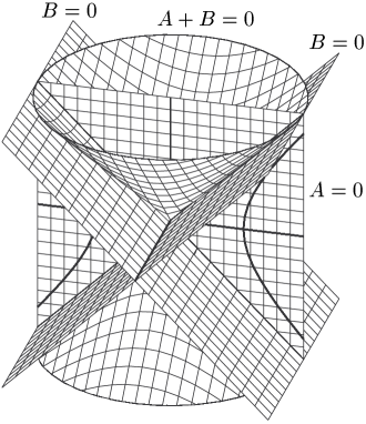
FIG. 1.: The general structure of boost-rotation symmetric spacetimes:
the axis – $A=0$,
the roof – $B=0$,
the null cone of the origin – $A+B=0$.

Since we wish to examine especially the radiative properties, let us concentrate on the region above the roof ($B<0$). We transform the Minkowski metric first to coordinates adapted to the boost-rotation symmetry $\{b,\ \rho,\ \phi,\ \chi\}$

$$x=\rho\cos\phi\ ,\mbox{\quad}y=\rho\sin\phi\ ,\mbox{\quad}z=b\sinh\chi\ ,\mbox{\quad}t=\pm\ b\cosh\chi$$ (61)

with $b\geq 0$, $\chi\in{\cal R}$, and further to null coordinates $u$, $v$

$$u=b-\rho\ ,\mbox{\quad}v=b+\rho\ .$$ (62)

The metric then takes the form

$${\rm d}s^{2}={\rm d}u{\rm d}v-{{\scriptstyle{\frac{1}{4}}}}(v^{2}-u^{2})\Bigl{[}\frac{v-u}{v+u}\ {\rm d}\phi^{2}+\frac{v+u}{v-u}\ {\rm d}\chi^{2}\Bigr{]}\ ,$$ (63)

where $v=u$ is the axis, $v=-u$ the roof, and the lines $u$, $\phi$, $\chi$ being constant, $v$ changing are null geodesics ending at null infinity ${\cal J}^{+}$ for $v\rightarrow+\infty$. The Killing vectors (60) are $\xi=\partial/\partial\phi$ and $\eta=\partial/\partial\chi$.

Inside the radiative part of the boost-rotation symmetric spacetime the boost Killing vector is spacelike. Thus one cannot distinguish between a small region of a curved boost-rotation symmetric spacetime and a small region of a curved cylindrically symmetric spacetime (one can transform a boost-rotation symmetric metric above the roof locally to the cylindrically symmetric Einstein-Rosen metric [34, 35]). However, these two spacetimes have essentially different asymptotical properties.

The null coordinates $u$, $v$ are related to canonical coordinates $U$, $V$ ($V={{\scriptstyle{\frac{1}{2}}}}v^{2}$ and $U={{\scriptstyle{\frac{1}{2}}}}u^{2}\ {\rm sign}\ u$) that can be used to distinguish between cylindrical and boost-rotation symmetry:
Proposition The metric of a curved spacetime admitting two spacelike, hypersurface orthogonal, commuting Killing vectors $\partial/\partial{\bar{x}}$ and $\partial/\partial{\bar{y}}$, and satisfying the vacuum Einstein equations can be, in a region where $W_{,\alpha}W^{,\alpha}$ does not change the sign, $W$ being the “volume element” of the group orbits, transformed into one of the following forms:

$${\rm d}s^{2}={\rm e}^{\Lambda}{\rm d}U{\rm d}V-W[{\rm e}^{-\Psi}{\rm d}{\bar{x}}^{2}+{\rm e}^{\Psi}{\rm d}{\bar{y}}^{2}]\ ,$$ (64)

where $\Lambda$, $\Psi$ are functions of $U$, $V$, and $W>0$ is such that

$$a) \ W={{\scriptstyle{\frac{1}{2}}}}(V+U)\ \mbox{ if }\ W,_{\alpha}\mbox{ is timelike},$$ (65)

$$b) \ W={{\scriptstyle{\frac{1}{2}}}}(V-U)\ \mbox{ if }\ W,_{\alpha}\mbox{ is spacelike},$$ (66)

$$c) \ \mbox{spacetimes with}\ W,_{\alpha}\ \mbox{null or}\ W=\mbox{const have more symmetries}.$$ (67)

The coordinates $U$ and $V$ are determined uniquely up to translations.

In a boost-rotation symmetric spacetime in radiative regions, $W,_{\alpha}$ is spacelike inside the null cone of the origin and timelike outside the null cone, whereas $W,_{\alpha}$ is spacelike everywhere in a cylindrically symmetric spacetime. The Killing vectors $\partial/\partial{\bar{x}}$ and $\partial/\partial{\bar{y}}$ are the axial and the boost Killing vector respectively.

The metric (63) can be generalized for a curved spacetime:
Definition 1 A spacetime admitting two spacelike, hypersurface orthogonal Killing vectors is called “boost-rotation symmetric” if in canonical coordinates ${{\scriptstyle{\frac{1}{2}}}}v^{2}$, ${{\scriptstyle{\frac{1}{2}}}}u^{2}$ (resp. $-{{\scriptstyle{\frac{1}{2}}}}u^{2}$ if $u<0$) the metric has the form

$${\rm d}s^{2}={\rm e}^{\lambda}\ {\rm d}u{\rm d}v-{{\scriptstyle{\frac{1}{4}}}}(v^{2}-u^{2})\Bigl{[}\frac{v-u}{v+u}\ {\rm e}^{-\mu}\ {\rm d}\phi^{2}+\frac{v+u}{v-u}\ {\rm e}^{\mu}\ {\rm d}\chi^{2}\Bigr{]}\ ,$$ (68)

$\phi\in\langle 0,\ 2\pi)$, $\chi\in{\cal R}$, the functions $\lambda(u,\ v)$, $\mu(u,\ v)$ are defined for $v\in(0<v_{0},\ +\infty)$, $u\in(u_{0},\ u_{1})$, $u<v$, $u\not=-v$, and

$$\lim_{{v\to\infty}\atop{u\ \mbox{{{fixed}}}}}\lambda(u,\ v)=\lambda_{0}(u)\ ,\mbox{\quad}\lim_{{v\to\infty}\atop{u\ \mbox{{{fixed}}}}}\mu(u,\ v)=\kappa=\mbox{const}\ .$$ (69)

This weaker asymptotic condition is compatible with the asymptotic flatness – boost-rotation symmetric spacetimes defined here admit a local ${\cal J}^{+}$. A stronger condition $\lambda\rightarrow 0$, $\mu\rightarrow 0$ as $v\rightarrow+\infty$ would imply a flat spacetime everywhere.

The boost-rotation symmetric metric defined in Def. 1 (68) above the roof, i.e., for $t^{2}>z^{2}$, can be extended to all values of “Cartesian-type” coordinates $\{t,\ x,\ y,\ z\}$ by transformations (61) and (62):
Definition 2 The boost-rotation symmetric vacuum solutions have the metric

$${\rm d}s^{2} = -(x^{2}+y^{2})^{-1}[{\rm e}^{\lambda}(x{\rm d}x+y{\rm d}y)^{2}+{\rm e}^{-\mu}(x{\rm d}y-y{\rm d}x)^{2}]-(z^{2}-t^{2})^{-1}[{\rm e}^{\lambda}(t{\rm d}t-z{\rm d}z)^{2}-{\rm e}^{\mu}(t{\rm d}z-z{\rm d}t)^{2}]$$ (70)

$$= -(x^{2}+y^{2})^{-1}[({\rm e}^{\lambda}x^{2}+{\rm e}^{-\mu}y^{2}){\rm d}x^{2}+2xy({\rm e}^{\lambda}-{\rm e}^{-\mu}){\rm d}x\ {\rm d}y+({\rm e}^{\lambda}y^{2}+{\rm e}^{-\mu}x^{2}){\rm d}y^{2}]$$ (72)

$$-(z^{2}-t^{2})^{-1}[({\rm e}^{\lambda}z^{2}-{\rm e}^{\mu}t^{2}){\rm d}z^{2}-2zt({\rm e}^{\lambda}-{\rm e}^{\mu}){\rm d}z\ {\rm d}t-({\rm e}^{\mu}z^{2}-{\rm e}^{\lambda}t^{2}){\rm d}t^{2}]\$$

with $(t,\ x,\ y,\ z)\in{\cal R}^{4}$, $x^{2}+y^{2}>0$, $z^{2}-t^{2}\not=0$, and

$$\mu=\mu(A=x^{2}+y^{2},\ B=z^{2}-t^{2})\ ,\mbox{\quad}\lambda=\lambda(A=x^{2}+y^{2},\ B=z^{2}-t^{2})\ .$$ (73)

The function $\mu$, determined up to an additive constant, is an analytic, asymptotically regular solution of the flat-space wave equation

$$\Box\mu=A\mu,_{AA}+B\mu,_{BB}+\mu,_{A}+\mu,_{B}=0$$ (74)

except for the regions where sources uniformly accelerated with respect to the Minkowskian background and defining $\mu$ occur. The function $\lambda$, determined up to an additive constant, is the solution of the field equations

$$(A+B)\lambda,_{A} = B(A{\mu,_{A}}^{2}-B{\mu,_{B}}^{2}+2A\mu,_{A}\mu,_{B})+(A-B)\mu,_{A}-2B\mu,_{B}\ ,$$ (75)

$$(A+B)\lambda,_{B} = A(B{\mu,_{B}}^{2}-A{\mu,_{A}}^{2}+2B\mu,_{A}\mu,_{B})+(A-B)\mu,_{B}+2A\mu,_{A}\$$ (76)

and it is analytic in all regions where $\mu$ is analytic, i.e., both are analytic even on the roof and everywhere on the axis outside the sources and nodal (conical) singularities which cause the particles to accelerate. The equation (74) is an integrability condition for equations (75) and (76).

One can see that $\mu$ and $\lambda$ (73) in canonical coordinates satisfy the boundary conditions required in Def. 1 and the metric admits the axial and boost Killing vectors which have the same form as in the Minkowski spacetime (60). Moreover, the structure of group orbits in the curved boost-rotation symmetric spacetime outside the sources or singularities is the same as the structure of axial and boost group orbits in the Minkowski spacetime. Thus the boost Killing vector is timelike below the roof, $z^{2}>t^{2}$, where the spacetime is stationary and there is no radiation. It is spacelike above the roof, $t^{2}>z^{2}$, where almost all null geodesics end and where the leading term of the Riemann tensor, proportional to $r^{-1}$ ($r^{2}=\rho^{2}+z^{2}$), is non-vanishing and has the same algebraic structure as in the case of plane waves. Consequently in regular regions of ${\cal J}$ above the roof the gravitational field is radiative.

This definition of vacuum boost-rotation symmetric spacetimes is “geometrical” by virtue of an invariant geometrical meaning of “Minkowskian” coordinates $\{t,\ x,\ y,\ z\}$ due to their relation to the canonical coordinates.

Using polar coordinates $\rho$, $\phi$ instead of $x$, $y$, the metric (72) becomes

$${\rm ds}^{2}=-{\rm e}^{\lambda}{\rm d}\rho^{2}-\rho^{2}{\rm e}^{-\mu}{\rm d}\phi^{2}-\frac{1}{z^{2}-t^{2}}\left[({\rm e}^{\lambda}z^{2}-{\rm e}^{\mu}t^{2}){\rm d}z^{2}-2zt({\rm e}^{\lambda}-{\rm e}^{\mu}){\rm d}z\ {\rm d}t+({\rm e}^{\lambda}t^{2}-{\rm e}^{\mu}z^{2}){\rm d}t^{2}\right]\ .$$ (77)

Since both the functions $\mu$ and $\lambda$ are determined up to an additive constant, we can make the roof regular, i.e.,

$$\mu(A,\ 0)=\lambda(A,\ 0)$$ (78)

is satisfied, by choosing the constants such that

$$\mu(0,0)=\lambda(0,0)\$$ (79)

is fulfilled as the Einstein equations (74)–(76) then imply (78). As the sources are located on the axis, we cannot make the whole axis regular but one can add the same constant to both $\mu$ and $\lambda$ to make parts of the axis regular, i.e., to satisfy

$$\mu(0,\ B)+\lambda(0,\ B)=0\ ,$$ (80)

and thus arrange the distribution of nodal (conical) singularities – “strings” – along the $z$-axis. One can make regular either the spatial infinity (then the string is between symmetrically located sources on the $z$-axis) or the axis between sources moving with opposite accelerations (then the string tends to infinity along the $z$-axis and thus propagates along null infinity to time infinity). Such solutions are asymptotically flat in the sense that they admit only local ${\cal J}$ (two generators are singular, or missing so that ${\cal J}^{\pm}\not\cong S^{2}\times{\cal R}$). See Sec. III for particular examples.

There are also solutions where no nodal singularity is necessary to cause the acceleration of the sources. Thus both the roof and axis (except for points where particles occur) are regular and the regularity conditions of the roof (79) and axis (80) at the origin imply $\mu(0,0)=\lambda(0,0)=0$. Both spacelike and timelike infinities are then regular. Null infinity ${\cal J}^{+}$ and ${\cal J}^{-}$ is regular except for four points, where the worldlines of sources “start” and “end” ($t=\pm z$, $z\rightarrow\pm\infty$) – the fixed points of the boost-rotation symmetry, i.e., the solution admits global null infinity in the sense of topology ${\cal J}^{\pm}\cong S^{2}\times{\cal R}$ though two generators are not complete. It can be shown that arbitrarily strong boost-rotation symmetric initial data can be prescribed on a hyperboloidal hypersurface above the roof leading to a complete smooth future null and timelike infinities. Here weak-field initial data are not necessary as in the proof of existence of general asymptotically flat radiative solutions (the work of Friedrich [36], Cutler and Wald [37], Christodoulou and Klainerman [38]). These exceptional cases can be represented by “self-accelerating” particles due to their multipole structure (an infinite number of these solutions is known in an explicit form [14]) or by several particles distributed symmetrically along the $z$-axis where negative masses have to be introduced (for example [13]).

“Generalized” boost-rotation symmetric solutions also do not contain singularities causing the acceleration and even no negative masses. They represent accelerated particles in external fields. The generalized C-metric was obtained by a certain procedure by Ernst [18], the generalized Bonnor-Swaminarayan solution was first constructed analogously and then in a more physical way as a limit of the asymptotically flat boost-rotation symmetric solution representing two accelerated pairs when the “outer” particle in each pair, attached to a string extending to infinity, goes to infinity with increasing mass parameter [39]. These solutions are the best rigorous known today examples of the motion of relativistic bodies, e.g., black holes in “external fields”. However, they are not asymptotically flat and thus it is difficult to analyze their radiative properties. In a limit of a weak external field, there are regions where radiation properties might be investigated since spacetimes are approximately flat there. Recently Hawking and Ross [40] used the generalized C-metric within the framework of quantum gravity. There exists also an electromagnetic generalization [19], where the charged black hole is accelerated by an external electric field (the same solution may be achieved by interacting electromagnetic and gravitational perturbations in a weak external limit [41]).

As was mentioned at the beginning, asymptotically flat boost-rotation symmetric spacetimes are the only non-trivial explicit exact radiative solutions representing moving objects and an analysis of their radiative properties may be helpful to understand physically more realistic situations. These solutions are the most realistic, although they contain nodal singularities or negative masses and their ADM mass vanishes, and thus can not serve as an example of a general spacetime with a positive ADM mass.

III Examples in electromagnetism and gravity

A Uniformly accelerated electromagnetic multipoles

In this section we study boost-rotation symmetric solutions of the Maxwell equations to gain better understanding of solutions with the same symmetries in general theory of relativity. The simplest case was studied first by Born [42]. It represents a field of two particles with opposite charges $\pm e$ symmetrically located and uniformly accelerated with a uniform acceleration $\pm\alpha^{-1}$, $\alpha>0$, along the $z$-axis of cylindrical coordinates $\{t,\rho,\phi,z\}$ in the Minkowski spacetime (see, e.g., [43]). They move independently of each other as they are separated by a null hypersurface, the roof (see Subsec. II B). Their worldlines are hyperbolas, integral curves of the timelike boost Killing vector,

$$\rho=0,\quad z_{(\pm e)}=\pm\sqrt{\alpha^{2}+t^{2}}\ .$$ (81)

A detailed analysis [43, 44] shows that the field can be interpreted as either the purely retarded field from the charge $+e$ in the region $z+t>0$ and the purely advanced field from the charge $-e$ in the region $z+t<0$, or as ${{\scriptstyle{\frac{1}{2}}}}$(advanced $+$ retarded) fields from both charges. However, the field is purely retarded in the region $t>|z|$ and purely advanced in $t<-|z|$. The same interpretation may be used for a field of uniformly accelerated electric [45] and magnetic [46, 47] multipoles.

The field of uniformly accelerated electric multipoles ($2^{l}-$poles) $\pm{\mathtt{e}}_{l}$ moving along hyperbolas (81) reads (see [45])

$$E^{(\rho)}_{(l)} = \enspace\ 8\ \frac{{\mathtt{e}}_{l}(2l-1)!!}{l!^{2}}\ \rho z\ \partial_{\alpha}^{(l)}\left({\frac{{\alpha}^{2}}{{\zeta}^{3}}}\right)\ ,\quad$$ (82)

$$E^{(z)}_{(l)} = -4\ \frac{{\mathtt{e}}_{l}(2l-1)!!}{l!^{2}}\ \partial_{\alpha}^{(l)}\left({\frac{{\alpha}^{2}\left({\alpha}^{2}+{t}^{2}+{\rho}^{2}-{z}^{2}\right)}{{\zeta}^{3}}}\right)\ ,$$ (83)

$$B^{(\phi)}_{(l)} = \enspace\ 8\ \frac{{\mathtt{e}}_{l}(2l-1)!!}{l!^{2}}\ \rho t\ \partial_{\alpha}^{(l)}\left({\frac{{\alpha}^{2}}{{\zeta}^{3}}}\right),$$ (84)

while the field corresponding to uniformly accelerated magnetic multipoles $\pm{\mathtt{m}}_{l}$ has the form (see [46, 47])

$$B^{(\rho)}_{(l)} = \enspace\ 8\ \frac{{\mathtt{m}}_{l}(2l-1)!!}{l!^{2}}\ \rho z\ \partial_{\alpha}^{(l)}\left({\frac{{\alpha}^{2}}{{\zeta}^{3}}}\right)\ ,$$ (85)

$$B^{(z)}_{(l)} = -4\ \frac{{\mathtt{m}}_{l}(2l-1)!!}{l!^{2}}\ \partial_{\alpha}^{(l)}\left({\frac{{\alpha}^{2}\left({\alpha}^{2}+{t}^{2}+{\rho}^{2}-{z}^{2}\right)}{{\zeta}^{3}}}\right)\ ,$$ (86)

$$E^{(\phi)}_{(l)} = -8\ \frac{{\mathtt{m}}_{l}(2l-1)!!}{l!^{2}}\ \rho t\ \partial_{\alpha}^{(l)}\left({\frac{{\alpha}^{2}}{{\zeta}^{3}}}\right),$$ (87)

where

$$\zeta=\sqrt{4\rho^{2}\alpha^{2}+(\alpha^{2}+t^{2}-z^{2}-\rho^{2})^{2}}\ .$$ (88)

The other field components vanish. It is obvious that the field given by (86) can be obtained from that given by (83) by a simple transformation

$$\vec{B}\rightarrow-\vec{E},\quad\vec{E}\rightarrow\vec{B}\ ,\quad{\mathtt{e}}_{l}\rightarrow{\mathtt{m}}_{l}\ ,$$ (89)

which is a special case of the duality symmetry.

Now let us analyze these solutions from the viewpoint of radiation. The Born solution, the simplest example of (83) representing the field of uniformly accelerated electric monopoles, was studied in some basic works by Pauli [48] and von Laue [49]. They considered the field as non-radiative as do some authors even now [50] (see also comments in [51, 52]). However, this is in a contradiction with the statement that an accelerated charge radiates energy with the rate $(2/3)e^{2}{\dot{v}}^{2}$. Performing a series expansion in $r^{-1}$ $(r^{2}=\rho^{2}+z^{2})$ with time $t$ fixed, the asymptotic behaviour of the Born field is $\vec{E}\sim r^{-4}$, $\vec{B}\sim r^{-5}$ and thus the Poynting vector $\vec{S}\sim r^{-9}$. In Fig. 2 we see that the quantities determining the field have the character of a pulse and it is therefore understandable why the Poynting vector $\vec{S}$ is non-radiative when going to spatial infinity and therefore passing through a pulse (see [44]). In the next part we will see that $\vec{S}\sim r^{-2}$ when travelling with the pulse with the velocity of light; then all fields (83) and (86) have a radiative character.

FIG. 2.: Pulse generated by a uniformly accelerated electric charge.

To examine the radiative properties of these solutions, we express the field components (83) and (86) in terms of spherical coordinates $(r,\theta,\phi)$ and of the retarded time of the origin $u=t-r$ and expand them in $r^{-1}$ with $u$, $\theta$, $\phi$ fixed (see [45, 46, 47]):

$$B^{(\rho)} = \enspace\ {\mathtt{m}}_{l}G_{l}\sin\theta\cos\theta\ \frac{1}{r}+{\cal O}(r^{-2})\ ,$$ (90)

$$B^{(z)} = -{\mathtt{m}}_{l}G_{l}\sin^{2}\theta\ \frac{1}{r}+{\cal O}(r^{-2})\ ,$$ (91)

$$E^{(\phi)} = -{\mathtt{m}}_{l}G_{l}\sin\theta\ \frac{1}{r}+{\cal O}(r^{-2})\ ,$$ (92)

where

$$G_{l}=\frac{(2l-1)!!}{l!^{2}}\ \partial_{\alpha}^{(l)}\left(\frac{\alpha^{2}}{(u^{2}+\alpha^{2}\sin^{2}\theta)^{3/2}}\right)\$$ (93)

and similarly for electric multipoles with respect to (89). Considering a particle with an arbitrary structure of electric and magnetic multipoles, the leading term of the radial component of the Poynting vector reads

$$S_{r}=\frac{\sin^{2}\theta}{4\pi r^{2}}\sum_{l,l^{\prime}}({\mathtt{e}}_{l}{\mathtt{e}}_{l^{\prime}}+{\mathtt{m}}_{l}{\mathtt{m}}_{l^{\prime}})G_{l}G_{l^{\prime}}+{\cal O}(r^{-3})\ .$$ (94)

Introducing the true retarded time $u^{*}$ of the particle by

$$t-u^{*}=|\vec{r}-\vec{r}^{\,*}|\ ,$$ (95)

where $(t,\vec{r})$ and $(u^{*},\vec{r}^{\,*})$ are the coordinates of an observation and emission event, respectively, we can express

$$u=u^{*}-\sqrt{{u^{*}}^{2}+\alpha^{2}}\cos\theta+{\cal O}(r^{-1})\ .$$ (96)

The radial flux emitted at $u^{*}=0$ thus takes the form

$$S_{r}=\frac{\sin^{2}\theta}{4\pi r^{2}}\sum_{l,l^{\prime}}\frac{(2l-1)!!(2l^{\prime}-1)!!({\mathtt{e}}_{l}{\mathtt{e}}_{l^{\prime}}+{\mathtt{m}}_{l}{\mathtt{m}}_{l^{\prime}})}{l!^{2}l^{\prime}!^{2}}\frac{V_{l}V_{l^{\prime}}}{\alpha^{l+l^{\prime}+2}}\ ,$$ (97)

where $V_{l}$ can be obtained by substituting (96) and $u^{*}=0$ into

$$\alpha^{l+1}\,\partial_{\alpha}^{(l)}\left(\frac{\alpha^{2}}{(u^{2}+\alpha^{2}\sin^{2}\theta)^{3/2}}\right)\ ;$$

thus $V_{0}=1$, $V_{1}=3\cos^{2}\theta-1$, $V_{2}=15\cos^{4}\theta-15\cos^{2}\theta+2$, $\dots$.
The total power radiated out, $R=2\pi\int_{0}^{\pi}{\lim\limits_{r\to\infty}}(r^{2}S_{r})\sin\theta\,{\rm d}\theta$, is then as follows

$$R=\sum_{l,l^{\prime}}R^{(l,l^{\prime})}\frac{{\mathtt{e}}_{l}{\mathtt{e}}_{l^{\prime}}+{\mathtt{m}}_{l}{\mathtt{m}}_{l^{\prime}}}{{\alpha^{l+l^{\prime}+2}}}\ ,$$ (98)

where $R^{(l,l^{\prime})}$ are introduced by (see (24) in [45])

$$R^{(l,l^{\prime})}=\frac{(2l-1)!!(2l^{\prime}-1)!!}{2l!^{2}l^{\prime}!^{2}}\int_{0}^{\pi}V_{l}V_{l^{\prime}}\sin^{3}\theta\,{\rm d}\theta\ .$$ (99)

This expression for the total radiated power (98) reduces to (23) in [45] when all ${\mathtt{m}}_{l}=0$. As in [45] we have $R^{(0,0)}=2/3$, $R^{(0,1)}=-4/15$, $R^{(1,1)}=8/21$, etc. Due to the boost symmetry, the particles radiate out energy (measured in an inertial frame in which the particle is at rest at the emission event) with a constant rate which is independent of $u^{*}$ and thus the same as at the turning point $u^{*}=0$. See [44] for the detailed discussion.

From (19), (47), and (48) it follows that radiative components of a general boost-rotation symmetric electromagnetic field tensor $F_{\mu\nu}$ in the coordinates $u$, $r$, $\theta$, $\phi$ are of the form

$$F_{u\theta} = X=\frac{{\cal E}(w)}{u^{2}}\ ,$$ (100)

$$F_{u\phi} = Y\sin\theta=\frac{\tilde{{\cal B}}(w)\sin\theta}{u^{2}}\ ,\mbox{\quad}{\rm where}\ \ w=\frac{\sin\theta}{u}\ .$$ (101)

Here $X$ and $Y$ correspond to the electromagnetic news functions of the system (see Subsubsec. II A 1 or [23, 7]). Notice that these radiative components are proportional to $r^{0}$ rather then to $r^{-1}$ due to the choice of coordinates. For a uniformly accelerated electric monopole (i.e., the Born solution) we obtain

$${\cal E}(w) = \frac{{\mathtt{e}}_{0}\alpha^{2}w}{(1+\alpha^{2}w^{2})^{3/2}}\mbox{\quad}\mbox{for}\ u>0\ ,\mbox{\quad}{\cal E}(w)=-\frac{{\mathtt{e}}_{0}\alpha^{2}w}{(1+\alpha^{2}w^{2})^{3/2}}\mbox{\quad}\mbox{for}\ u<0\ ,$$ (102)

$$\tilde{{\cal B}}(w) = 0.$$ (103)

For a uniformly accelerated electric dipole we get

$${\cal E}(w) = \frac{{\mathtt{e}}_{1}\alpha w(2-\alpha^{2}w^{2})}{(1+\alpha^{2}w^{2})^{5/2}}\mbox{\quad}\mbox{for}\ u>0\ ,\mbox{\quad}{\cal E}(w)=-\frac{{\mathtt{e}}_{1}\alpha w(2-\alpha^{2}w^{2})}{(1+\alpha^{2}w^{2})^{5/2}}\mbox{\quad}\mbox{for}\ u<0\ ,$$ (104)

$$\tilde{{\cal B}}(w) = 0\ ,$$ (105)

whereas for a magnetic dipole one finds

$${\cal E}(w) = 0\ ,$$ (106)

$$\tilde{{\cal B}}(w) = -\frac{{\mathtt{m}}_{1}\alpha w(2-\alpha^{2}w^{2})}{(1+\alpha^{2}w^{2})^{5/2}}\mbox{\quad}\mbox{for}\ u>0\ ,\mbox{\quad}\tilde{{\cal B}}(w)=\frac{{\mathtt{m}}_{1}\alpha w(2-\alpha^{2}w^{2})}{(1+\alpha^{2}w^{2})^{5/2}}\mbox{\quad}\mbox{for}\ u<0\ .$$ (107)

For a general electric $2^{l}$-pole the news functions turn out to be

$${\cal E}(w) = {\mathtt{e}}_{l}(G_{l}u^{3})w\ ,$$ (108)

$$\tilde{{\cal B}}(w) = 0\ ,$$ (109)

while for a magnetic $2^{l}$-pole

$${\cal E}(w) = 0\ ,$$ (110)

$$\tilde{{\cal B}}(w) = -{\mathtt{m}}_{l}(G_{l}u^{3})w$$ (111)

with $G_{l}$ given by (93).

One can check that the total electric and magnetic charges (27) for the general electric and magnetic multipoles vanish,

$$\int\limits_{0}^{\pi}({\cal E}\cos\theta/u){\rm d}\theta=0\ ,\mbox{\quad}\int\limits_{0}^{\pi}(\tilde{{\cal B}}\cos\theta/u){\rm d}\theta=0\ .$$ (112)

B The Bonnor-Swaminarayan solutions

In 1957 Bondi [53] proved the existence of an axially symmetric solution of the Einstein equations corresponding to two pairs of particles having equal masses but of opposite sign uniformly accelerated in opposite directions. Seven years later Bonnor and Swaminarayan constructed such a solution explicitly [13]. Particles in this solution – point singularities of Curzon-Chazy type (see [35]) – move freely and the acceleration force is caused by mutual gravitational interaction. They obtained also other similar metrics, some of them representing only positive masses. However, particles considered there do not move freely, line singularities of a conical type, interpreted as nodes, rods, struts or stresses, always appear.

Since Bonnor-Swaminarayan solutions (BS-solutions) are boost-rotation symmetric, their metrics have, in cylindrical coordinates $t$, $\rho$, $z$, and $\phi$, the form (77), in which the functions entering the metric read

$$\mu = -\frac{2a_{1}}{R_{1}}-\frac{2a_{2}}{R_{2}}+\frac{2a_{1}}{h_{1}}+\frac{2a_{2}}{h_{2}}+\ln k\ ,$$ (113)

$$\lambda = \frac{a_{1}a_{2}}{(h_{1}-h_{2})^{2}}f-\rho^{2}(z^{2}-t^{2})\biggl{(}\frac{a_{1}^{2}}{R_{1}^{4}}+\frac{a_{2}^{2}}{R_{2}^{4}}\biggr{)}+\frac{2a_{1}R}{h_{1}R_{1}}+\frac{2a_{2}R}{h_{2}R_{2}}+\ln k\ ,$$ (114)

$$R = {{\scriptstyle{\frac{1}{2}}}}(\rho^{2}+z^{2}-t^{2})\ ,$$ (115)

$$R_{i} = \sqrt{(R-h_{i})^{2}+2\rho^{2}h_{i}}\ ,\mbox{\quad}i=1,2\ ,$$ (116)

$$f = \frac{4}{R_{1}R_{2}}[\rho^{2}(z^{2}-t^{2})+(R-\rho^{2}-h_{1})(R-\rho^{2}-h_{2})-R_{1}R_{2}]\ ,$$ (117)

where $a_{1}$, $a_{2}$, $h_{1}>0$, $h_{2}>0$, $k>0$ are constants.

The whole class of BS-solutions describes the gravitational field of a finite number of monopole Curzon-Chazy particles (CC-particles) uniformly accelerated in opposite directions where the acceleration force is caused by a gravitational interaction among particles or by nodal singularities. Let us now study two examples separately.

1 The Bonnor-Swaminarayan solution representing two pairs of freely moving CC-particles without a nodal singularity

The simplest case without a nodal singularity is the BS-solution, considered first by Bondi, containing two pairs of freely falling particles: there is one particle with positive and one with negative mass in each pair. In this case the constant parameters in (115) are given by

$$a_{1}=\frac{(h_{1}-h_{2})^{2}}{2h_{2}}\ ,\mbox{\quad}a_{2}=-\frac{(h_{1}-h_{2})^{2}}{2h_{1}}\ ,\mbox{\quad}k=1\ .$$ (118)

To examine the radiative properties and to find the news function of this solution, we shall transform the metric at first to spherical flat-space coordinates $\{R,\ \vartheta,\ \phi\}$ by $\rho=R\sin\vartheta$, $z=R\cos\vartheta$, $\phi=\phi$, and flat-space retarded time $U=t-R$ (see [44]) and then find a transformation to the Bondi coordinates $u$, $r$, $\theta$, and $\phi$, where the metric has the Bondi form (see (5) or [21] and (2), (4) in [44]).

For $h_{2}=h$, $h_{1}=h+{\tilde{\epsilon}}$, ${\tilde{\epsilon}}>0$ small, $k=1$ we obtain a slightly curved spacetime with the masses given by $m^{(1)}={\tilde{\epsilon}}^{2}/[2h\sqrt{2h+2{\tilde{\epsilon}}}]$, $m^{(2)}=-{\tilde{\epsilon}}^{2}/[(2h+2{\tilde{\epsilon}})\sqrt{2h}]$. The relation between the flat coordinates $\{U,\ R,\ \vartheta,\ \phi\}$ and the Bondi coordinates $\{u,\ r,\ \theta,\ \phi\}$ is then (see [44])

$$U=[u+{\cal O}({\tilde{\epsilon}}^{3})]+{\cal O}(r^{-1})\ ,\mbox{\quad}R=r+{\cal O}(1)\ ,\mbox{\quad}\vartheta=\theta+{\cal O}(r^{-1})\ ,\mbox{\quad}\phi=\phi\ .$$ (119)

The only non-vanishing news function of this system in the Bondi coordinates, neglecting higher terms in $\epsilon$, reads

$$c,_{u} = {\tilde{\epsilon}}^{3}\frac{3u\sin^{2}\theta}{2h(u^{2}+2h\sin^{2}\theta)^{5/2}}\$$ (120)

$$= {\tilde{\epsilon}}^{3}\frac{3w^{2}}{2h(1+2hw^{2})^{5/2}}\frac{1}{u^{2}}\mbox{\quad}{\rm{for}}\ u>0\ ,$$ (121)

$$= -{\tilde{\epsilon}}^{3}\frac{3w^{2}}{2h(1+2hw^{2})^{5/2}}\frac{1}{u^{2}}\mbox{\quad}{\rm{for}}\ u<0\ ,\mbox{\quad}{\rm{where}}\mbox{\quad}w=\frac{\sin\theta}{u}\ .$$ (122)

One obtains the same news function (up to a constant) for another solution found in [14] as was shown in [54]. It is constructed from the BS-solution representing two pairs of particles uniformly accelerated along the symmetry axis in opposite directions and containing one positive and one negative mass connected by a nodal singularity (this case was not considered explicitly in [13]). A limiting procedure that brings particles in each pair together simultaneously increasing their masses leads to a field representing two independent self accelerating (0,1)-pole CC-particles called “monodiperos” (the monopole and dipole parts are present in the field function). Except for places where particles occur, the spacetime is regular. An octupole radiation pattern was demonstrated for the BS-solution representing freely moving CC-particles in [44] and for the field of monodiperos in [54].

Comparing (122) with the news function corresponding to a general asymptotically flat boost-rotation symmetric solution of the Einstein equations (44), one sees that

$${{\cal K}},_{w}(w) = \ {\tilde{\epsilon}}^{3}\frac{3w^{2}}{2h(1+2hw^{2})^{5/2}}\mbox{\quad}{\rm{for}}\mbox{\quad}u>0\ ,$$ (123)

$${{\cal K}},_{w}(w) = -{\tilde{\epsilon}}^{3}\frac{3w^{2}}{2h(1+2hw^{2})^{5/2}}\mbox{\quad}{\rm{for}}\mbox{\quad}u<0\ .$$ (124)

Then solving Eq. (53) for the function $\lambda(w)$ and substituting the result into Eq. (46), we finally integrate Eq. (56) to get the total Bondi mass at ${\cal J}^{+}$

$$m = \frac{{\bar{\epsilon}}^{2}u^{3}(5u^{4}+32u^{2}h+64h^{2})}{4h^{7/2}(u^{2}+2h)^{7/2}}\sqrt{2}\times\Bigl{[}-\ln(u^{2})+\ln\left|-2\sqrt{2h}\sqrt{u^{2}+2h}+u^{2}+4h\right|\Bigr{]}$$ (125)

$$+\frac{{\bar{\epsilon}}^{2}(u^{2}+4h)(15u^{4}+16u^{2}h+32h^{2})}{3h^{3}u(u^{2}+2h)^{3}}\ ,\mbox{\quad}{\bar{\epsilon}}=\frac{3{\tilde{\epsilon}}^{3}}{2^{6}h}\ .$$ (126)

In Fig. 3a we see that the Bondi mass $m$ (126) as a function of $u$ is everywhere decreasing and thus the system does radiate gravitational waves. One can easily verify that the axis is regular here, i.e., $c,_{u}/\sin^{2}\theta$ is a regular function in the limit $\sin\theta\ \rightarrow\ 0$. Fig. 3b contains a radiation pattern of this solution at the turning point, i.e., a polar diagram of the function $c,_{u}^{2}(\theta,\ u^{*}=0)$ (see (96) for the definition of $u^{*}$) – a gravitational radiation flow to different directions at the turning point.

FIG. 3.: Two pairs of freely moving CC-particles:
a) the decrease of the total Bondi mass at ${\cal J}^{+}$ (126) and
b) the radiation pattern emitted at the turning point $u^{*}=0$.

2 The Bonnor-Swaminarayan solution representing two CC-particles connected with a nodal singularity

Another example of a boost-rotation symmetric solution is the BS-solution (77), (115) describing two symmetrically located CC-particles, uniformly accelerated in opposite directions and connected with a conical singularity of a finite length given by the constants

$$\ln k=-4mA\ ,\mbox{\quad}a_{1}=\frac{m}{A}\ ,\mbox{\quad}h_{1}=\frac{1}{2A^{2}}\ ,\mbox{\quad}a_{2}=h_{2}=0\ .$$ (127)

As in the previous case we transform the metric first to flat-space coordinates $\{U,\ R,\ \vartheta,\ \phi\}$ and then to the Bondi coordinates $\{u,\ r,\ \theta,\ \phi\}$ that are connected in limits of small mass $mA\ll 1$ and $r\rightarrow\infty$ by

$$U=[u+{\cal O}(mA)]+{\cal O}(r^{-1})\ ,\mbox{\quad}R=r+{\cal O}(1)\ ,\mbox{\quad}\vartheta=\theta+{\cal O}(r^{-1})\ ,\mbox{\quad}\phi=\phi\ .$$ (128)

Then the news function in the Bondi coordinates reads (see (28) in [55])

$$c,_{u} = \frac{2mA}{\sin^{2}\theta}+\frac{mu}{A(u^{2}+\sin^{2}\theta/A^{2})^{3/2}}+\frac{2mAu}{\sin^{2}\theta\sqrt{u^{2}+\sin^{2}\theta/A^{2}}}$$ (129)

$$= \biggl{[}\frac{2mA}{w^{2}}+\frac{m}{A(1+w^{2}/A^{2})^{3/2}}+\frac{2mA}{w^{2}\sqrt{1+w^{2}/A^{2}}}\biggr{]}\frac{1}{u^{2}}\mbox{\quad}{\rm{for}}\ u>0\ ,$$ (130)

$$= \biggl{[}\frac{2mA}{w^{2}}-\frac{m}{A(1+w^{2}/A^{2})^{3/2}}-\frac{2mA}{w^{2}\sqrt{1+w^{2}/A^{2}}}\biggr{]}\frac{1}{u^{2}}\mbox{\quad}{\rm{for}}\ u<0\ ,$$ (131)

with $w=\sin\theta/u$ and thus the function ${\cal K},_{w}(w)$ in (44) reads

$${\cal K},_{w}(w) = \frac{2mA}{w^{2}}+\frac{m}{A(1+w^{2}/A^{2})^{3/2}}+\frac{2mA}{w^{2}\sqrt{1+w^{2}/A^{2}}}\mbox{\quad}{\rm{for}}\ u>0\ ,$$ (132)

$${\cal K},_{w}(w) = \frac{2mA}{w^{2}}-\frac{m}{A(1+w^{2}/A^{2})^{3/2}}-\frac{2mA}{w^{2}\sqrt{1+w^{2}/A^{2}}}\mbox{\quad}{\rm{for}}\ u<0\ .$$ (133)

Following the same procedure as in the previous case, fairly long calculations lead to the total Bondi mass (it is finite only for $u<0$ where the news function is regular)

$$m = \frac{1}{8}\frac{m^{2}A^{2}\left|u\right|\ln(A\left|u\right|)(16+15A^{2}u^{2})}{(A^{2}u^{2}+1)^{3/2}}-4m^{2}A^{2}\left|u\right|\ln(A\left|u\right|)+2m^{2}A^{2}\left|u\right|\ln(A^{2}u^{2}+1)$$ (135)

$$\ -\frac{1}{16}\frac{m^{2}A^{2}\left|u\right|\ln(A^{2}u^{2}+2+2\sqrt{A^{2}u^{2}+1})(16+15A^{2}u^{2})}{(A^{2}u^{2}+1)^{3/2}}-\frac{1}{8}\frac{m^{2}(A^{2}u^{2}+2)}{(A^{2}u^{2}+1)\left|u\right|}\ .$$

In the regular part of the spacetime, for $u<0$, the dependence of $m$ as a function of $u$ is qualitatively the same as in the previous case in Fig. 3. This solution has the axis regular only for $u<0$ where $c,_{u}/\sin^{2}\theta$ is a regular function in the limit $\sin\theta\ \rightarrow\ 0$.

C The C-metric

1 Introduction

The C-metric was originally discovered in 1917 by Levi-Civita [11] and Weyl [12]. This algebraically degenerate vacuum solution of Petrov type D was called C-metric by Ehlers and Kundt [56] and its geometrical properties were studied in [57]. Electromagnetic generalization of the C-metric was discovered in 1970 by Kinnersley and Walker [58], who also first noticed that it includes not only static regions when it is analytically continued. In the early 80’s Ashtekar and Dray [59] showed that the C-metric is asymptotically flat at spatial infinity and admits smooth cross-sections of null infinity. As the original coordinate system corresponds to the special algebraic structure of the solution, it was necessary to transform the C-metric into other coordinates where physical properties can be examined (see [58, 60]). In 1983 Bonnor [61] transformed the C-metric into the Weyl coordinates and further into coordinates adapted to boost and rotation symmetries (77) where also a radiative part of the spacetime appears. Bonnor showed that the C-metric could be regarded as the metric of two Schwarzschild black holes with a string causing them to move with a uniform acceleration. It is necessary to perform long calculations to express metric coefficients in terms of the Weyl coordinates. In [62] Bonnor showed that the charged C-metric with $m=0$ corresponds, in the weak field limit, to the electromagnetic Born solution describing uniformly accelerated charges (see Subsec. III A). In 1995 Cornish and Uttley [63] found that the C-metric in the form (136) contains four different spacetimes. Recently Yongcheng [64] derived the C-metric from the metric of two superposed Schwarzschild black holes assuming that the mass and location of one of them approaches infinity in an appropriate way. In 1998 Tomimatsu studied power-law decay of the tails of gravitational radiation at future null infinity for the C-metric and Wells [65] proved the black hole uniqueness theorem for it.

The C-metric is a solution of the Einstein vacuum equations and in coordinates $\{x$, $y$, $p$, $\tau\}$ it has the form [58]

$${\rm d}s^{2}=\frac{1}{A^{2}(x+y)^{2}}\left(F^{-1}{\rm d}y^{2}+G^{-1}{\rm d}x^{2}+G{\rm d}p^{2}-F{\rm d}\tau^{2}\right)\ ,$$ (136)

where the functions $F$, $G$ are cubic polynomials

$$F = -1+y^{2}-2mAy^{3}\ ,$$ (137)

$$G = \ \ 1-x^{2}-2mAx^{3}\ ,$$ (138)

with $m$ and $A$ being constant. We suppose that the condition $27m^{2}A^{2}<1$ is satisfied, which implies that $F$, $G$ have three distinct real roots $y_{1}$, $y_{2}$, $y_{3}$ and $x_{1}$, $x_{2}$, $x_{3}$.

2 Transformation of the C-metric into the Weyl form

The metric (136) has two Killing vectors ($\partial/\partial\tau$ and $\partial/\partial p$) and it can be transformed into the Weyl form in specific regions. Weyl solutions are static, axially symmetric spacetimes with the metric

$${\rm d}s^{2}={\rm e}^{-2U}\left[{\rm e}^{2\nu}({\rm d}{\bar{\rho}}^{2}+{\rm d}{\bar{z}}^{2})+{\bar{\rho}}^{2}{\rm d}\bar{\phi}^{2}\right]-{\rm e}^{2U}{\rm d}{\bar{t}}^{2}\ ,$$ (139)

where the functions $U({\bar{\rho}},{\bar{z}})$ and $\nu({\bar{\rho}},{\bar{z}})$ are to be determined from the Einstein vacuum equations

$$0 = \frac{\partial^{2}U}{\partial{\bar{\rho}}^{2}}+\frac{1}{{\bar{\rho}}}\frac{\partial U}{\partial{\bar{\rho}}}+\frac{\partial^{2}U}{\partial{\bar{z}}^{2}}\ ,$$ (140)

$$\frac{1}{{\bar{\rho}}}\frac{\partial\nu}{\partial{\bar{\rho}}} = \left(\frac{\partial U}{\partial{\bar{\rho}}}\right)^{2}-\left(\frac{\partial U}{\partial{\bar{z}}}\right)^{2}\ ,$$ (141)

$$\frac{1}{{\bar{\rho}}}\frac{\partial\nu}{\partial{\bar{z}}} = 2\frac{\partial U}{\partial{\bar{\rho}}}\frac{\partial U}{\partial{\bar{z}}}\ .$$ (142)

The first equation in (141) is the integrability condition for the other two ones. If the $\bar{z}$-axis given by $\bar{\rho}=0$ is regular, then for every infinitesimal circle around it the ratio of circumference to radius is $2\pi$ and thus the Minkowski space exists locally. The regularity condition reads

$${\rm e}^{2\nu}(\bar{\rho}=0,\bar{z})=1.$$ (143)

A conical singularity appears on the $\bar{z}-$axis if the regularity condition (143) is not satisfied.

Using relations (see [61]) ${\bar{t}}=\tau$, ${\bar{\varphi}}=p$, and

$${\bar{z}} = \frac{1+mAxy(x-y)+xy}{A^{2}(x+y)^{2}}\ ,$$ (144)

$${\bar{\rho}}^{2} = \frac{FG}{A^{4}(x+y)^{4}}\ ,$$ (145)

one can transform the C-metric (136) into the Weyl form (139). It follows that the metric functions ${\rm e}^{2U}$ and ${\rm e}^{2\nu}$ are then given by

$${\rm e}^{2U} = \frac{F}{A^{2}(x+y)^{2}}\ ,$$ (146)

$${\rm e}^{2\nu} = \frac{1}{A^{4}(x+y)^{4}\left[\left(\frac{\partial{\bar{z}}}{\partial y}\right)^{2}+\left(\frac{\partial{\bar{\rho}}}{\partial y}\right)^{2}\right]}\ .$$ (147)

In order to express these functions in coordinates $\bar{\rho}$ and $\bar{z}$, we have to invert relations (144) and (145) and substitute $x=x({\bar{\rho}},{\bar{z}})$ and $y=y({\bar{\rho}},{\bar{z}})$ into (146) and (147).

It is convenient to introduce functions $R_{i}$, $i=1,2,3$, defined by

$$R_{i}=\sqrt{({\bar{z}}-z_{i})^{2}+{\bar{\rho}}^{2}}\ ,$$ (148)

where $z_{1}<z_{2}<z_{3}$ are the roots of the equation

$$2A^{4}{z_{i}}^{3}-A^{2}{z_{i}}^{2}+m^{2}=0\ .$$ (149)

The functions $R_{i}$ satisfy relations [61]

$${R_{i}}^{2}=\left(\frac{m(Az_{i})^{-1}+A^{2}z_{i}(x-y)-mAxy}{A^{2}(x+y)}\right)^{2}\ ,$$ (150)

which, taking a square root, become

$${R_{i}}=\epsilon_{i}\left(\frac{m(Az_{i})^{-1}+A^{2}z_{i}(x-y)-mAxy}{A^{2}(x+y)}\right)$$ (151)

with $\epsilon_{1}$, $\epsilon_{2}$, $\epsilon_{3}=\pm 1$ to be chosen in such a way that the right-hand sides of (151) are positive. Thus, all $\epsilon_{i}$ depend on $x$ and $y$.

Now one can express $x$ and $y$ in terms of $\bar{\rho}$, $\bar{z}$

$$x = \frac{F_{0}+F_{1}}{2F_{2}}\ ,$$ (152)

$$y = \frac{F_{0}-F_{1}}{2F_{2}}\ ,$$ (153)

where

$$F_{0} = \epsilon_{1}\epsilon_{2}\epsilon_{3}m(z_{1}-z_{2})(z_{2}-z_{3})(z_{3}-z_{1})\ ,$$ (154)

$$F_{1} = -m\left[\epsilon_{1}\epsilon_{2}(z_{1}-z_{2})z_{3}R_{3}+\epsilon_{2}\epsilon_{3}(z_{2}-z_{3})z_{1}R_{1}+\epsilon_{3}\epsilon_{1}(z_{3}-z_{1})z_{2}R_{2}\right]\ ,$$ (155)

$$F_{2} = \frac{m^{2}}{2A}\left[\epsilon_{1}\epsilon_{2}(z_{1}-z_{2})R_{3}+\epsilon_{2}\epsilon_{3}(z_{2}-z_{3})R_{1}+\epsilon_{3}\epsilon_{1}(z_{3}-z_{1})R_{2}\right]\ .$$ (156)

Substituting the equations (152), (153) into (146), (147), we get the metric functions ${\rm e}^{2U}$ and ${\rm e}^{2\nu}$ in terms of the Weyl coordinates $\bar{\rho}$ and $\bar{z}$. Since there are eight different choices for $\epsilon_{1}$, $\epsilon_{2}$, and $\epsilon_{3}$, there are in principle eight different Weyl spacetimes contained in (136). Four of them have signature $+2$ and the remaining four $-2$. Later we will consider some of these combinations explicitly.

3 Properties of the C-metric in the original coordinates $x$, $y$ and in the Weyl coordinates

The metric (136) has signature $+2$ if $G>0$ and signature $-2$ if $G<0$. We choose signature $+2$ and thus we investigate only regions where $G>0$. The Killing vector $\partial/\partial\tau$=$\partial/\partial\bar{t}$ is timelike (and thus spacetime is static) for $F>0$. The character of various regions is illustrated in Fig. 4. Notice that Fig. 4 is only schematic in the sense that the squares have the same size, although the intervals between the roots (or roots and infinity) are not the same.

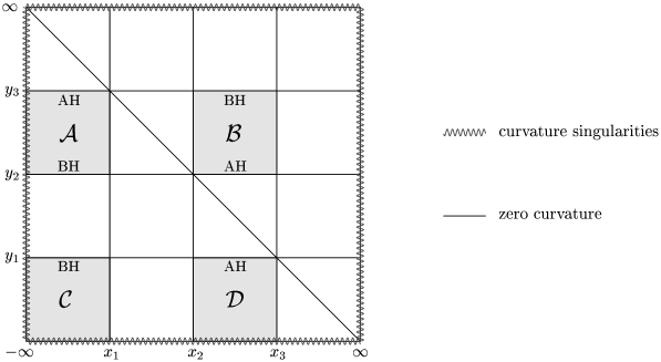
FIG. 4.: The character of the regions determined by roots of polynomials $F$ and $G$ is schematically illustrated. Static regions are shaded, black hole horizons are denoted by BH and acceleration horizons by AH. Curvature singularities and points with zero curvature are also marked.

As was mentioned in [63], the C-metric in the $x$, $y$ coordinates contains four various static regions with signature $+2$. These regions, denoted by ${\cal{A,\ B,\ C,\ D,}}$ have the following values of $\epsilon_{i}$:

$$\epsilon_{1}=-1,\quad\epsilon_{2}=-1,\quad\ \epsilon_{3}=+1\quad{\mbox{in the~{}region }}\ {\cal A},$$ (157)

$$\epsilon_{1}=-1,\quad\epsilon_{2}=+1,\quad\ \epsilon_{3}=-1\quad{\mbox{in the~{}region }}\ {\cal B},$$ (158)

$$\epsilon_{1}=+1,\quad\epsilon_{2}=+1,\quad\ \epsilon_{3}=+1\quad{\mbox{in the~{}region }}\ {\cal C},$$ (159)

$$\epsilon_{1}=+1,\quad\epsilon_{2}=-1,\quad\ \epsilon_{3}=-1\quad{\mbox{in the~{}region }}\ {\cal D},$$ (160)

and thus they can be transformed into different Weyl forms by the transformation (144) and (145).

Now let us analyze singularities of the metric (136). For this purpose it is useful to calculate several simple invariants of the Riemann tensor :

$$I_{1} = {R^{\alpha\beta}}_{\gamma\delta}{R_{\alpha\beta}}^{\gamma\delta}=-48m^{2}A^{6}(x+y)^{6}\ ,$$ (161)

$$I_{2} = {R^{\alpha\beta}}_{\gamma\delta}{R^{\gamma\delta}}_{\varepsilon\lambda}{R^{\varepsilon\lambda}}_{\alpha\beta}=-96m^{3}A^{9}(x+y)^{9}\ ,$$ (162)

$$I_{3} = R^{\alpha\beta\gamma\delta}R_{\alpha\varepsilon\lambda\mu}{R^{\varepsilon\lambda}}_{\beta\nu}{R^{\mu\nu}}_{\gamma\delta}=-144m^{4}A^{12}(x+y)^{12}\ .$$ (163)

A spacetime can be flat only at those points where curvature invariants are approaching zero. Expressions (162) thus indicate that asymptotically flat regions can exist only on a line given by

$$x+y=0\ .$$ (164)

Singularities of the curvature invariants (162) are located at the points $x+y\rightarrow\infty$ and marked in Fig. 4.

From (145) it follows that if $F$ or $G$ vanishes, then the Weyl coordinate $\bar{\rho}$ is equal to zero. Thus Eq. (145) maps the boundaries ($x=x_{i}$, $\pm\infty$) or ($y=y_{i}$, $\pm\infty$) onto the $\bar{z}-$axis of the Weyl coordinates. Note that as the  Weyl coordinates describe only the static part of the spacetime there are regions of the $\bar{z}$-axis corresponding to black hole horizons or acceleration horizons. These segments of the $\bar{z}$-axis do not correspond to the real, smooth physical axis.

The Killing vector $\partial/\partial\tau$ of the metric (136) is timelike inside the four regions ${\cal{A,\ B,\ C,\ D,}}$ but it has a zero norm at the boundaries $y=y_{i}$ and thus the Killing horizons are located there. To distinguish between the acceleration horizons and black hole horizons, one can calculate the area of each horizon [66]:

$$\int\limits_{0}^{2\pi}\int\limits_{x_{k}}^{x_{k+1}}\sqrt{g_{\bar{\varphi}\bar{\varphi}}}\sqrt{g_{xx}}{\rm d}x{\rm d}\bar{\varphi}=\frac{2\pi}{A^{2}}\int\limits_{x_{k}}^{x_{k+1}}\frac{{\rm d}x}{(x+y_{j})^{2}}=\frac{2\pi}{A^{2}}\frac{x_{k+1}-x_{k}}{(x_{k}+y_{j})(x_{k+1}+y_{j})}\ ,$$ (165)

where $j=1,\dots,3$, $k=0,1,\dots,4$, $x_{0}=-\infty$, and $x_{4}=\infty$. A horizon of a black hole has a finite area whereas an acceleration horizon has an infinite area. Locations of these horizons are indicated in Fig. 4.

Each region ${\cal{A,\ B,\ C,\ D}}$ corresponds to a different Weyl metric (see (169)–(174)). Properties of the $\bar{z}$-axis in the Weyl coordinates are illustrated in Fig. 5.

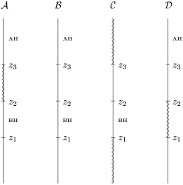
FIG. 5.: The $\bar{z}$-axis in the Weyl coordinates for cases ${\cal{A,\ B,\ C,\ D}}$.

There is no horizon and curvature singularity between points $z_{2}$ and $z_{3}$ in the cases ${\cal{B,\ C,\ D}}$, however, in general, the  axis is not regular there because of a conical singularity (see Eq. (143)). The same is true for ${\cal{A,\ B,\ D}}$ and $\bar{z}<z_{1}$.

There is no acceleration horizon in the spacetime ${\cal{C}}$, and so this case does not represent uniformly accelerated sources. Moreover, this spacetime is not asymptotically flat because curvature invariants (162) are everywhere non-vanishing and thus we will not study this case further.

If functions ${\rm e}^{-2U}$ and ${\rm e}^{2\nu}$ satisfy the field equations (141), then the same do also functions

$${\rm e}^{-2U^{\prime}} = a\ {\rm e}^{-2U}\ ,$$ (166)

$${\rm e}^{2\nu^{\prime}} = b\ {\rm e}^{2\nu}\$$ (167)

for $a$ and $b$ being constant. This solution is for $a^{2}\not=b^{2}$ indeed a new solution and cannot be transformed into the initial one by a coordinate transformation since a curvature invariant, which is coordinate independent, satisfies

$${R^{\prime}}_{\alpha\beta\gamma\delta}{R^{\prime}}^{\alpha\beta\gamma\delta}=\frac{a^{2}}{b^{2}}{R}_{\alpha\beta\gamma\delta}{R}^{\alpha\beta\gamma\delta}\ .$$ (168)

Later we will use (166) to construct a solution which is regular for ${\bar{z}}<z_{1}$ or for $z_{2}<{\bar{z}}<z_{3}$ in the cases where there is no curvature singularity.

Finally, let us express the functions ${\rm e}^{2U}$ and ${\rm e}^{2\nu}$ in terms of ${\bar{\rho}}$, ${\bar{z}}$ by substituting (152), (153) into (146), (147) (see [61] for the case ${\cal B}$):

$${\rm e}^{2U}_{\cal A} = \frac{\left[R_{1}-(\bar{z}-z_{1})\right]\left[R_{2}-(\bar{z}-z_{2})\right]}{R_{3}-(\bar{z}-z_{3})}\quad{\mbox{in the~{}region}}\ {\cal A},$$ (169)

$${\rm e}^{2U}_{\cal B} = \frac{\left[R_{1}-(\bar{z}-z_{1})\right]\left[R_{3}-(\bar{z}-z_{3})\right]}{R_{2}-(\bar{z}-z_{2})}\quad{\mbox{in the~{}region}}\ {\cal B},$$ (170)

$${\rm e}^{2U}_{\cal D} = \frac{\left[R_{2}-(\bar{z}-z_{2})\right]\left[R_{3}-(\bar{z}-z_{3})\right]}{R_{1}-(\bar{z}-z_{1})}\quad{\mbox{in the~{}region}}\ {\cal D},$$ (171)

and

$${\rm e}^{2\nu}_{\cal A} = \frac{1}{4}\frac{m^{2}}{A^{6}(z_{3}-z_{1})^{2}(z_{3}-z_{2})^{2}}\frac{\left[R_{2}R_{3}+{\bar{\rho}}^{2}+({\bar{z}}-z_{2})({\bar{z}}-z_{3})\right]\left[R_{3}R_{1}+{\bar{\rho}}^{2}+({\bar{z}}-z_{3})({\bar{z}}-z_{1})\right]}{R_{1}R_{2}R_{3}\left[R_{1}R_{2}+{\bar{\rho}}^{2}+({\bar{z}}-z_{1})({\bar{z}}-z_{2})\right]}\ {\rm e}^{2U}_{\cal A}\ ,$$ (172)

$${\rm e}^{2\nu}_{\cal B} = \frac{1}{4}\frac{m^{2}}{A^{6}(z_{2}-z_{1})^{2}(z_{3}-z_{2})^{2}}\frac{\left[R_{2}R_{3}+{\bar{\rho}}^{2}+({\bar{z}}-z_{2})({\bar{z}}-z_{3})\right]\left[R_{1}R_{2}+{\bar{\rho}}^{2}+({\bar{z}}-z_{1})({\bar{z}}-z_{2})\right]}{R_{1}R_{2}R_{3}\left[R_{1}R_{3}+{\bar{\rho}}^{2}+({\bar{z}}-z_{1})({\bar{z}}-z_{3})\right]}\ {\rm e}^{2U}_{\cal B}\ ,$$ (173)

$${\rm e}^{2\nu}_{\cal D} = \frac{1}{4}\frac{m^{2}}{A^{6}(z_{1}-z_{2})^{2}(z_{1}-z_{3})^{2}}\frac{\left[R_{1}R_{2}+{\bar{\rho}}^{2}+({\bar{z}}-z_{1})({\bar{z}}-z_{2})\right]\left[R_{1}R_{3}+{\bar{\rho}}^{2}+({\bar{z}}-z_{1})({\bar{z}}-z_{3})\right]}{R_{1}R_{2}R_{3}\left[R_{2}R_{3}+{\bar{\rho}}^{2}+({\bar{z}}-z_{2})({\bar{z}}-z_{3})\right]}\ {\rm e}^{2U}_{\cal D}\ .$$ (174)

4 The C-metric in the canonical coordinates adapted to the boost-rotation symmetry

Following Bonnor [61], we shall transform the metric from the Weyl coordinates to new coordinates in which the boost-rotation symmetry of the C-metric is evident. Performing an analytical continuation of the resulting metric, two new regions of the spacetime will appear.

The metric of a general boost-rotation symmetric spacetime in polar coordinates $\{t$, $\rho$, $z$, $\phi\}$ has the form (77) and the transformation

$$\bar{z}-z_{3} = {{\scriptstyle{\frac{1}{2}}}}(t^{2}+\rho^{2}-z^{2})\ ,$$ (175)

$${\bar{\rho}}^{2} = \rho^{2}(z^{2}-t^{2})\ ,$$ (176)

$$\bar{t} = {\mbox{arctanh}}(t/z)\ ,$$ (177)

$$\bar{\phi} = \phi$$ (178)

brings the metric (139) into this form with

$${\rm e}^{\mu}=\frac{{\rm e}^{2U}}{z^{2}-t^{2}}\ ,\quad{\rm e}^{\lambda}=\frac{{\rm e}^{2\nu}}{{\rm e}^{2U}}(\rho^{2}+z^{2}-t^{2})\ .$$ (179)

Applying the transformation (176), the functions $R_{1}$, $R_{2}$, $R_{3}$ (148) turn to be

$$R_{1} = \sqrt{(R+Z_{1})^{2}-2Z_{1}\rho^{2}}\ ,$$ (180)

$$R_{2} = \sqrt{(R+Z_{2})^{2}-2Z_{2}\rho^{2}}\ ,$$ (181)

$$R_{3} = R\ ,$$ (182)

where

$$R = {{\scriptstyle{\frac{1}{2}}}}(z^{2}-t^{2}+\rho^{2})\ ,$$ (183)

$$Z_{1} = z_{1}-z_{3}\ ,$$ (184)

$$Z_{2} = z_{2}-z_{3}\ .$$ (185)

The functions ${\rm e}^{\mu}$ and ${\rm e}^{\lambda}$ are then given by

$${\rm{\rm e}}^{\mu}_{\cal{A}} = \frac{(R_{1}+R+Z_{1}-\rho^{2})(R_{2}+R+Z_{2}-\rho^{2})}{(z^{2}-t^{2})^{2}}\ ,$$ (186)

$${\rm{\rm e}}^{\mu}_{\cal{B}} = \frac{R_{1}+R+Z_{1}-\rho^{2}}{R_{2}+R+Z_{2}-\rho^{2}}\ ,$$ (187)

$${\rm e}^{\mu}_{\cal{D}} = \frac{R_{2}+R+Z_{2}-\rho^{2}}{R_{1}+R+Z_{1}-\rho^{2}}\ ,$$ (188)

and

$${\rm e}^{\lambda}_{\cal{A}} = \frac{1}{2}\frac{m^{2}}{A^{6}{Z_{1}}^{2}{Z_{2}}^{2}}\frac{\left[R(R_{2}+R+Z_{2})-Z_{2}\rho^{2}\right]\left[R(R_{1}+R+Z_{1})-Z_{1}\rho^{2}\right]}{R_{1}R_{2}\left[R_{1}R_{2}+(R+Z_{1})(R+Z_{2})-(Z_{1}+Z_{2})\rho^{2}\right]}\ ,$$ (189)

$${\rm e}^{\lambda}_{\cal{B}} = \frac{1}{2}\frac{m^{2}}{A^{6}{(Z_{2}-Z_{1})}^{2}{Z_{2}}^{2}}\frac{\left[R(R_{2}+R+Z_{2})-Z_{2}\rho^{2}\right]\left[R_{1}R_{2}+(R+Z_{1})(R+Z_{2})-(Z_{1}+Z_{2})\rho^{2}\right]}{R_{1}R_{2}\left[R(R_{1}+R+Z_{1})-Z_{1}\rho^{2}\right]}\ ,$$ (190)

$${\rm e}^{\lambda}_{\cal{D}} = \frac{1}{2}\frac{m^{2}}{A^{6}{(Z_{2}-Z_{1})}^{2}{Z_{1}}^{2}}\frac{\left[R(R_{1}+R+Z_{1})-Z_{1}\rho^{2}\right]\left[R_{1}R_{2}+(R+Z_{1})(R+Z_{2})-(Z_{1}+Z_{2})\rho^{2}\right]}{R_{1}R_{2}\left[R(R_{2}+R+Z_{2})-Z_{2}\rho^{2}\right]}\ .$$ (191)

Let us recall the regularity condition of the metric (77) on the roof (78)

$${\rm e}^{\mu}={\rm e}^{\lambda}\mbox{\quad}{\mbox{ for }}\mbox{\quad}z^{2}=t^{2}\ ,$$ (192)

and the regularity condition of the axis (80)

$$\lim_{\rho\to 0}{\rm e}^{\lambda}{\rm e}^{\mu}=1\ .$$ (193)

There are three regions on the $z$-axis

region I: $$z^{2}-t^{2}<-2Z_{2}\quad\dots\quad{\mbox{between particles}},$$ (194)

region II: $$-2Z_{2}<z^{2}-t^{2}<-2Z_{1}\quad\dots\quad{\mbox{particles}},$$ (195)

region III: $$z^{2}-t^{2}>-2Z_{1}\quad\dots\quad{\mbox{outside particles}}.$$ (196)

Using the multiplicative freedom described by Eq. (166) for the metric (77) with (186), (189) in the region ${\cal A}$, i.e., with

$${\rm e}^{\mu} = \alpha\gamma\frac{(R_{1}+R+Z_{1}-\rho^{2})(R_{2}+R+Z_{2}-\rho^{2})}{(z^{2}-t^{2})^{2}}\ ,$$ (197)

$${\rm e}^{\lambda} = \beta\gamma\frac{\left[R(R_{2}+R+Z_{2})-Z_{2}\rho^{2}\right]\left[R(R_{1}+R+Z_{1})-Z_{1}\rho^{2}\right]}{R_{1}R_{2}\left[R_{1}R_{2}+(R+Z_{1})(R+Z_{2})-(Z_{1}+Z_{2})\rho^{2}\right]}\ ,$$ (198)

we may construct solutions which are regular on the whole roof and on a part of the $z$-axis (between or outside particles) as has been done in [67, 46]. This can be arranged by appropriately chosen constants $\alpha$, $\beta$, $\gamma$. The regularity condition on the roof (192) implies

$$\alpha=2\beta\quad{\mbox{and}}\mbox{\quad}Z_{1}<0\ ,\mbox{\quad}Z_{2}<0\ .$$ (199)

To analyze the regularity of the axis, the following limits of functions ${\rm e}^{\mu}$ and ${\rm e}^{\lambda}$ for $\rho\to 0$ will be needed:

$$\lim_{\rho\to 0}{\rm e}^{\mu} = 0\ ,\hskip 113.81102pt\lim_{\rho\to 0}{\rm e}^{\lambda}=0\hskip 113.81102pt{\mbox{ in the~{}region I}},$$ (200)

$$\lim_{\rho\to 0}{\rm e}^{\mu} = 0\ ,\hskip 113.81102pt\lim_{\rho\to 0}{\rm e}^{\lambda}=-2\,{\frac{\beta\gamma{Z_{1}}^{2}\left(2Z_{2}+B\right)}{\left(2Z_{1}+B\right)\left(Z_{1}-Z_{2}\right)^{2}}}\mbox{\quad}{\mbox{ in the~{}region II}},$$ (201)

$$\lim_{\rho\to 0}{\rm e}^{\mu} = {\frac{\alpha\gamma\left(2Z_{1}+B\right)\left(2Z_{2}+B\right)}{B^{2}}}\ ,\mbox{\quad}\lim_{\rho\to 0}{\rm e}^{\lambda}=2\,{\frac{{B}^{2}\gamma\beta}{\left(2\,Z_{1}+B\right)\left(2\,Z_{2}+B\right)}}\mbox{\quad}\hskip 8.0pt{\mbox{ in the~{}region III}},$$ (202)

where $B=z^{2}-t^{2}$ is defined in (60). Thus the only part of the axis which can be regularized is the region III (outside black holes) with

$$\alpha=1\ ,\mbox{\quad}\beta=\frac{1}{2}\ ,\mbox{\quad}\gamma=\pm 1\ ,$$ (203)

and then the type ${\cal A}$ solution given by (197), (198) describes two uniformly accelerated black holes connected by a curvature singularity. The rest of the axis is regular (see Fig. 6).

FIG. 6.: The type ${\cal A}$ solution for $\alpha=1$, $\beta=1/2$, $\gamma=\pm 1$ describes two uniformly accelerated black holes connected by a curvature singularity.

We use the same procedure in the case ${\cal B}$ (187), (190):

$${\rm e}^{\mu} = \alpha\gamma\frac{R_{1}+R+Z_{1}-\rho^{2}}{R_{2}+R+Z_{2}-\rho^{2}}\ ,$$ (204)

$${\rm e}^{\lambda} = \beta\gamma\frac{\left[R(R_{2}+R+Z_{2})-Z_{2}\rho^{2}\right]\left[R_{1}R_{2}+(R+Z_{1})(R+Z_{2})-(Z_{1}+Z_{2})\rho^{2}\right]}{R_{1}R_{2}\left[R(R_{1}+R+Z_{1})-Z_{1}\rho^{2}\right]}\$$ (205)

to determine constants $\alpha$, $\beta$, and $\gamma$ regularizing the roof and parts of the axis. We find that for

$$\alpha=1\ ,\mbox{\quad}\beta=\frac{1}{2}\ ,\mbox{\quad}\gamma=\pm 1\mbox{\quad}{\mbox{the~{}region III is regular}},$$ (206)

and the C-metric of the type ${\cal B}$ describes two black holes connected by a conical singularity, with the rest of the axis being regular (see Fig. 7a). For values

$$\alpha=1\ ,\mbox{\quad}\beta=\frac{1}{2}\ ,\mbox{\quad}\gamma=\pm\frac{Z_{1}}{Z_{2}}\mbox{\quad}{\mbox{the~{}region I is regular}},$$ (207)

and this case describes two uniformly accelerated black holes with conical singularities which are extending from black holes to infinity. The axis is regular between the black holes (see Fig. 7b).

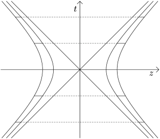
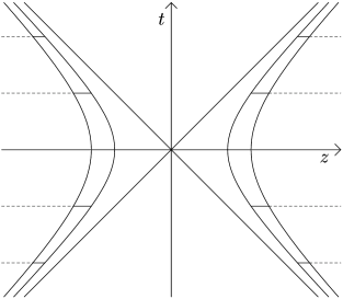
FIG. 7.: The C-metric of the type ${\cal B}$ with $\alpha=1$, $\beta=1/2$, and
a) with $\gamma=\pm 1$ describes two uniformly accelerated black holes connected by a conical singularity;
b) with $\gamma=\pm Z_{1}/Z_{2}$ describes two uniformly accelerated black holes with conical singularities extending to infinity.

In the ${\cal D}$-case (188), (191), i.e., for functions ${\rm e}^{\mu}$ and ${\rm e}^{\lambda}$ being

$${\rm e}^{\mu} = \alpha\gamma\frac{R_{2}+R+Z_{2}-\rho^{2}}{R_{1}+R+Z_{1}-\rho^{2}}\ ,$$ (208)

$${\rm e}^{\lambda} = \beta\gamma\frac{\left[R(R_{1}+R+Z_{1})-Z_{1}\rho^{2}\right]\left[R_{1}R_{2}+(R+Z_{1})(R+Z_{2})-(Z_{1}+Z_{2})\rho^{2}\right]}{R_{1}R_{2}\left[R(R_{2}+R+Z_{2})-Z_{2}\rho^{2}\right]}\ ,$$ (209)

the axis is regular in the region III for values

$$\alpha=1,\ \beta=\frac{1}{2},\ \gamma=\pm 1\ .$$ (210)

Then the C-metric of the type ${\cal D}$ describes two uniformly accelerated curvature singularities connected by a conical singularity. The rest of the axis is regular (see Fig. 8a). The axis is regular in the region I for values

$$\alpha=1,\ \beta=\frac{1}{2},\ \gamma=\pm\frac{Z_{2}}{Z_{1}}\ ,$$ (211)

that corresponds to two uniformly accelerated curvature singularities with conical singularities extending to infinity. The axis between curvature singularities is regular (see Fig. 8b).

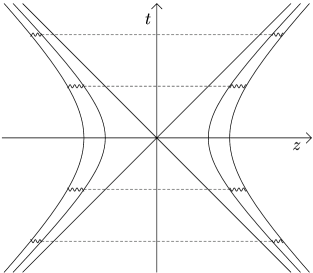
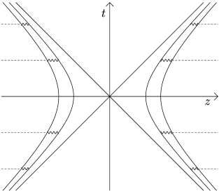
FIG. 8.: The C-metric of the type ${\cal D}$ with $\alpha=1$, $\beta=1/2$, and
a) with $\gamma=\pm 1$ corresponds to two uniformly accelerated curvature singularities connected by a conical singularity;
b) with $\gamma=\pm Z_{2}/Z_{1}$ describes two uniformly accelerated curvature singularities with conical singularities which are extended to infinity.

5 The news function

In further we calculate the news function, $c,_{u}$, which characterizes gravitational radiation radiated out to null infinity (see Subsubsec. II A 1), in the most realistic case of the C-metric, the type ${\cal B}$. It is probably possible to express it explicitly only in a limit of small masses of the sources. Introducing flat-space spherical coordinates

$$\rho=R\sin\vartheta\ ,\mbox{\quad}z=R\cos\vartheta\ ,\mbox{\quad}t=U+R\ ,$$ (212)

and expanding ${\rm e}^{\mu}$ and ${\rm e}^{\lambda}$ (205) in powers of ${R}^{-1}$, with $U$, $\vartheta$, $\phi$ fixed, one gets

$${\rm e}^{\mu} = \alpha\gamma\left[1+\frac{1}{\sin^{2}\vartheta}\left({\sqrt{U^{2}-2Z_{2}\sin^{2}\vartheta}}-{\sqrt{U^{2}-2Z_{1}\sin^{2}\vartheta}}\right)\frac{1}{R}\right]+{\cal O}\left(R^{-2}\right)\ ,$$ (213)

$${\rm e}^{\lambda} = \beta\gamma\frac{\left[U(U-U_{2})-Z_{2}\sin^{2}\vartheta\right]\left[U^{2}-(Z_{1}+Z_{2})\sin^{2}\vartheta+U_{1}U_{2}\right]}{U_{1}U_{2}\left[U(U-U_{1})-Z_{1}\sin^{2}\vartheta\right]}+{\cal O}\left(R^{-1}\right)\ ,\$$ (214)

where

$$U_{1}={\sqrt{U^{2}-2Z_{1}\sin^{2}\vartheta}}\ ,\mbox{\quad}U_{2}={\sqrt{U^{2}-2Z_{2}\sin^{2}\vartheta}}\ ,$$ (215)

and for small $m$

$$Z_{1}=-\frac{1}{2A^{2}}-\frac{m}{A}+{\cal O}(m^{2})\ ,\mbox{\quad}Z_{2}=-\frac{1}{2A^{2}}+\frac{m}{A}+{\cal O}(m^{2})\ .$$ (216)

Performing an expansion for small mass $m$ (with $A$ fixed), the relations (213) and (214) yield

$${\rm e}^{\mu} = \alpha\gamma\left(1-\frac{2m}{\sqrt{A^{2}U^{2}+\sin^{2}\vartheta}}\frac{1}{R}\right)\ ,$$ (217)

$${\rm e}^{\lambda} = 2\gamma\beta-8\gamma\beta mA\sin^{2}\vartheta\frac{\sin^{2}\ \vartheta-UA\sqrt{A^{2}U^{2}+\sin^{2}\vartheta}+A^{2}U^{2}}{\left(A^{2}U^{2}+\sin^{2}\vartheta\right)\left(2U^{2}A^{2}-2UA\sqrt{A^{2}U^{2}+\sin^{2}\vartheta}+\sin^{2}\vartheta\right)}\ .$$ (218)

Considering a conical singularity only between particles, i.e., putting $\alpha=1$, $\beta=1/2$, $\gamma=1$ and following Sec. 4 in [44], we introduce functions $\bar{\alpha}(U,\vartheta)$ and $\bar{B}(U,\vartheta)$ by

$${\rm e}^{\mu} = 1+\frac{\bar{\alpha}}{R}+{\cal O}(R^{-2})\ ,$$ (219)

$${\rm e}^{\lambda} = \bar{B}+{\cal O}(R^{-1})\ ,$$ (220)

where

$$\bar{\alpha} = -\frac{2m}{\sqrt{A^{2}U^{2}+\sin^{2}\vartheta}}\ ,$$ (221)

$$\bar{B} = 1-4mA\sin^{2}\vartheta\frac{\sin^{2}\ \vartheta-UA\sqrt{A^{2}U^{2}+\sin^{2}\vartheta}+A^{2}U^{2}}{\left(A^{2}U^{2}+\sin^{2}\vartheta\right)\left(2U^{2}A^{2}-2UA\sqrt{A^{2}U^{2}+\sin^{2}\vartheta}+\sin^{2}\vartheta\right)}\ .$$ (222)

In order to analyze radiative properties of the system, we move to the Bondi coordinates $u$, $r$, $\theta$, $\phi$ (see Subsubsec. II A 1) connected by an asymptotic transformation (see [44])

$$U = \pi^{0}(u,\theta)+{\cal O}\left(r^{-1}\right)\ ,$$ (223)

$$R = r+{\cal O}({r}^{0})\ ,$$ (224)

$$\vartheta = \theta+{\cal O}\left(r^{-1}\right)\ ,$$ (225)

where $\int{\bar{B}}(\pi^{0},\theta){\mbox{d}}\pi^{0}=u$, and for small $m$ one gets $\pi^{0}=u$ and thus $U=u$. To express the news function we use the relation (26) of Ref. [44]

$$c,_{u}=\frac{1-\bar{B}+{\bar{\alpha}},_{U}\sin^{2}\vartheta}{2\bar{B}\sin^{2}\vartheta}$$ (226)

which is valid for a general boost-rotation symmetric spacetime that is asymptotically flat, does not contain an infinite cosmic string, and has hypersurface orthogonal Killing vectors as was shown in [54]. Then the news function for the  ${\cal B}$-type C-metric regularized outside the particles is, in terms of $w=\sin\theta/u$, given by [67, 46]

$$c,_{u} = {\frac{-mA\left(A-2\,\sqrt{{A}^{2}+{w}^{2}}\right)w^{2}}{{u}^{2}\left({A}^{2}+{w}^{2}\right)^{3/2}\left(2\,{A}^{2}-2\,\sqrt{{A}^{2}+{w}^{2}}A+{w}^{2}\right)}}\quad{\mbox{for $u>0$}}\ ,$$ (227)

$$c,_{u} = {\frac{mA\left(A+2\,\sqrt{{A}^{2}+{w}^{2}}\right)w^{2}}{{u}^{2}\left({A}^{2}+{w}^{2}\right)^{3/2}\left(2\,{A}^{2}+2\,\sqrt{{A}^{2}+{w}^{2}}A+{w}^{2}\right)}}\quad{\mbox{for $u<0$}}\ .$$ (228)

This is in agreement with the expression (44) obtained in [7] for a general boost rotation symmetric spacetime. The news function is regular for $u<0$ and the total Bondi mass calculated there has qualitatively the same dependence on $u$ as in the BS-solutions (see Subsec. III B and Fig. 3a therein). The news function is singular for $u>0$ at $\theta=0,\ \pi$ due to a conical singularity connecting the particles (recall that we assume $A>0$).

D The spinning C-metric

The spinning C-metric (SC-metric), a generalization of the C-metric with the rotation, NUT parameter, and electric and magnetic charges, was found by Plebański and Demiański [16] in 1976 in the coordinates $\{\tau$, $p$, $q$, $\sigma\}$

$${{\rm d}s}^{2}={\frac{E\left(Q-P{q}^{4}\right)}{F}}\ {{{\rm d}\tau}}^{2}-\ {\frac{EF}{Q}}\ {{\rm d}q}^{2}-\ {\frac{EF}{P}}\ {{\rm d}p}^{2}+\ {\frac{E\left(Q{p}^{4}-P\right)}{F}}\ {{\rm d}\sigma}^{2}-\ {\frac{2\,E\left(Q{p}^{2}+P{q}^{2}\right)}{F}}\ {\rm d}\tau{\rm d}\sigma\ ,$$ (229)

where

$$P = \ \ \gamma-{\varepsilon}\,{p}^{2}+2\,m{p}^{3}-\gamma{p}^{4}\ ,$$ (230)

$$Q = -\gamma+{\varepsilon}\,{q}^{2}+2\,m{q}^{3}+\gamma{q}^{4}\ ,$$ (231)

$$E = \left(p+q\right)^{-2}\ ,$$ (232)

$$F = 1+{p}^{2}{q}^{2}\ ,$$ (233)

$m$, $\gamma$, $\varepsilon$ being constant. Here we put the parameters corresponding to the NUT parameter, electric and magnetic charges, and cosmological constant, $n$, $e$, $g$, $\lambda$ respectively, equal to zero, however, in the general form of the Plebański-Demiański metric (Eqs. (2.1), (3.25) in [16]) they are non-vanishing. They also demonstrated that the standard C-metric (136) or the Kerr metric can be obtained from (229) by specific limiting procedures. This metric was later analyzed by Farhoosh and Zimmerman [60], and recently discussed by Letelier and Oliveira [66].

Hereafter we assume the polynomials $P$ and $Q$ to have four distinct real roots (the corresponding conditions for $m$, $\varepsilon$ and $\gamma$ are given in [17]).

The metric (229) having two Killing vectors,

$${\frac{\partial}{\partial\tau}}\quad{\rm and}\quad{\frac{\partial}{\partial\sigma}}\ ,$$ (234)

was transformed into coordinates adapted to boost-rotation symmetry in [17]. However, the corresponding Killing vectors are not hypersurface orthogonal and thus the general theory summarized in Subsec. II B cannot be applied to this case and until now no similar general theory is available for the boost-rotation symmetric spacetimes with Killing vectors which are not hypersurface orthogonal.

1 The SC-metric in the Weyl-Papapetrou coordinates

As was shown in [17] the SC-metric (229) can be converted by a transformation

$${{\rm d}\tau} = {\kappa_{1}}\,{{\rm d}\bar{t}}+{\kappa_{2}}\,{{\rm d}\bar{\phi}}\ ,$$ (235)

$${{\rm d}\sigma} = {\kappa_{3}}\,{{\rm d}\bar{t}}+{\kappa_{4}}\,{{\rm d}\bar{\phi}}$$ (236)

with constants $\kappa_{1}\dots\kappa_{4}$ and

$${\bar{\rho}}^{2} = {E}^{2}{\cal K}^{2}PQ\ ,\ \ \ {\cal K}=\left({\kappa_{2}}\,{\kappa_{3}}-{\kappa_{1}}\,{\kappa_{4}}\right)\ ,$$ (237)

$$\bar{z} = {\cal K}{\frac{-\gamma-\varepsilon\,qp-m{q}^{2}p+mq{p}^{2}+\gamma{q}^{2}{p}^{2}}{(p+q)^{2}}}\$$ (238)

into the standard Weyl-Papapetrou form

$${\rm d}s^{2}={\rm e}^{-2U}\left[{{\rm e}^{2\nu}}({{\rm d}\bar{\rho}}^{2}+{{{\rm d}\bar{z}}}^{2})+{\bar{\rho}}^{2}{{{\rm d}\bar{\phi}}}^{2}\right]-{{\rm e}^{2\,U}}\left({{\rm d}\bar{t}}+a{{\rm d}\bar{\phi}}\right)^{2}\ ,$$ (239)

where $\bar{\phi}\in\langle 0,2\pi)$, $\bar{\rho}\in\langle 0,\infty)$, $\bar{t},\bar{z}\in R$ and functions $U$, $\nu$, $a$ depend only on $\bar{\rho}$ and $\bar{z}$. The metric functions satisfy the vacuum Einstein equations

$$0 = \frac{\partial^{2}U}{\partial\bar{z}^{2}}+\frac{1}{\bar{\rho}}\frac{\partial U}{\partial\bar{\rho}}+\frac{\partial^{2}U}{\partial\bar{\rho}^{2}}+\frac{1}{2}\frac{{\rm e}^{4U}}{\bar{\rho}^{2}}\left[\left(\frac{\partial a}{\partial\bar{\rho}}\right)^{2}+\left(\frac{\partial a}{\partial\bar{z}}\right)^{2}\right]\ ,$$ (240)

$$0 = \frac{\partial}{\partial\bar{z}}\left(\frac{{\rm e}^{4U}}{{\bar{\rho}}}\frac{\partial a}{\partial\bar{z}}\right)+\frac{\partial}{\partial{\bar{\rho}}}\left(\frac{{\rm e}^{4U}}{{\bar{\rho}}}\frac{\partial a}{\partial{\bar{\rho}}}\right)\ ,$$ (241)

$$\frac{1}{{\bar{\rho}}}\frac{\partial\nu}{\partial{\bar{\rho}}} = \left(\frac{\partial U}{\partial{\bar{\rho}}}\right)^{2}-\left(\frac{\partial U}{\partial\bar{z}}\right)^{2}-\frac{{\rm e}^{4U}}{4{\bar{\rho}}^{2}}\left[\left(\frac{\partial a}{\partial{\bar{\rho}}}\right)^{2}-\left(\frac{\partial a}{\partial\bar{z}}\right)^{2}\right]\ ,$$ (242)

$$\frac{1}{{\bar{\rho}}}\frac{\partial\nu}{\partial\bar{z}} = 2\frac{\partial U}{\partial{\bar{\rho}}}\frac{\partial U}{\partial\bar{z}}-\frac{{\rm e}^{4U}}{2{\bar{\rho}}^{2}}\frac{\partial a}{\partial{\bar{\rho}}}\frac{\partial a}{\partial\bar{z}}\ .$$ (243)

Notice that analogically to the non-rotating case, the $\bar{z}$-axis of the Weyl-Papapetrou coordinates (${\bar{\rho}}=0$) is a real smooth geometrical (physical) axis only at points where the metric (239) satisfies the regularity conditions

$$\lim_{{\bar{\rho}}\to\infty}\frac{X_{,\alpha}X^{,\alpha}}{4X}=1\ ,\ {\rm where}\ X=\xi_{(\bar{\phi})\alpha}\xi_{(\bar{\phi})}^{\alpha}\ ,\mbox{\quad}\xi_{(\bar{\phi})}=\frac{\partial}{\partial\bar{\phi}}\ .$$ (244)

Some parts of the axis may represent either a horizon of a rotating black hole or a rotating string and thus the regularity conditions (244) are not satisfied.

2 Properties of the SC-metric in the $p$, $q$ coordinates

In [17] the character of the Killing vectors (234) and their linear combinations with constant coefficients $k_{1}$, $k_{2}$,

$$\eta=k_{1}\frac{\partial}{\partial\tau}+k_{2}\frac{\partial}{\partial\sigma}\ ,$$ (245)

is studied. There exists a linear combination (245) that is spacelike and another one which is timelike in regions where

$$PQ>0\ ,$$ (246)

and thus the spacetime is stationary there.

The metric (229) has the signature $-2$ for $P>0$, whereas $P<0$ implies signature $+2$. Following [17] we choose the signature $+2$, i.e., $P<0$.

The curvature invariant

$$I = R^{\alpha\beta\gamma\delta}R_{\alpha\varepsilon\lambda\mu}{R^{\varepsilon\lambda}}_{\beta\nu}{R^{\mu\nu}}_{\gamma\delta}=-144m^{4}\frac{(p+q)^{12}}{(1+p^{2}q^{2})^{6}}\$$ (247)

indicates that asymptotically flat regions can exist only on the line given by $p+q=0$ and the curvature singularities are located at points $[p,q]=[0,\infty]$, $[0,-\infty]$, $[-\infty,0]$, $[\infty,0]$, where the invariant (247) diverges.

These results are summarized in Fig. 9, where $p_{1}<p_{2}<p_{3}<p_{4}$ and $q_{1}<q_{2}<q_{3}<q_{4}$ denote the roots of the polynomials $P$ and $Q$, and the numbers $1,\ \dots,\ 5$ indicate regions between individual roots or between a root and infinity. Stationary regions with the signature $+2$ are shaded, the diagonal line corresponds to the asymptotically flat regions and each curvature singularity is indicated by a cross. A detailed analysis (see [17]) shows that the left edge of the picture has to be identified with the right one and the bottom edge with the upper one as well. Notice that lines $p=p_{i}$ or $q=q_{i}$ are mapped onto the $\bar{z}$-axis of the Weyl coordinates due to the relation (237).

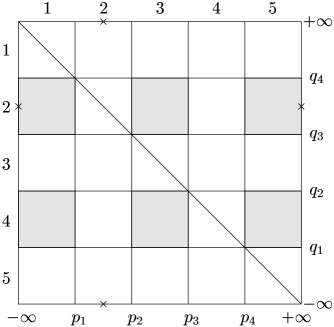
FIG. 9.: The schematic illustration of the SC-metric in the $p$, $q$ coordinates.

Further we concentrate on the square $\{2,3\}$ with $p\in\langle p_{2},p_{3}\rangle$, $q\in\langle q_{3},q_{4}\rangle$ as in [17]. The detailed analysis in [17] determines the location of the black hole horizon, the acceleration horizon, and the geometrical axis on the ${\bar{z}}$-axis of the Weyl coordinates along which the string represented by a conical singularity may lay (see Fig. 10). The vortices are marked by ${\bar{z}}_{i}$, the values of which follow from (238). The lower left vortex $L$ has a special property: when it is approached along the left edge of the square we arrive at ${\bar{z}}\rightarrow-\infty$, along the bottom edge at ${\bar{z}}\rightarrow+\infty$ and by approaching it along different lines from the interior of the square, we can achieve various values of ${\bar{\rho}}$ and ${\bar{z}}$.

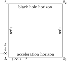
FIG. 10.: The square $\{2,3\}$ from Fig. 9.

3 The SC-metric in the canonical coordinates adapted to the boost-rotation symmetry

The Weyl-Papapetrou coordinates cover only stationary regions of the SC-metric (shadowed squares in Fig. 9). The  transformation (176) brings the metric (239) into the form in which the boost-rotation symmetry of the SC-metric will become manifest

$${\rm ds}^{2} = {\rm e}^{\lambda}{\rm d}\rho^{2}+\rho^{2}{\rm e}^{-\mu}{\rm d}\phi^{2}+\frac{1}{z^{2}-t^{2}}\left[({\rm e}^{\lambda}z^{2}-{\rm e}^{\mu}t^{2}){\rm d}z^{2}-2zt({\rm e}^{\lambda}-{\rm e}^{\mu}){\rm d}z{\rm d}t+({\rm e}^{\lambda}t^{2}-{\rm e}^{\mu}z^{2}){\rm d}t^{2}\right]$$ (249)

$$-2a{\rm e}^{\mu}(z{\rm d}t-t{\rm d}z){\rm d}\phi-a^{2}{\rm e}^{\mu}(z^{2}-t^{2}){\rm d}\phi^{2}\ ,$$

where ${\rm e}^{\mu}$ and ${\rm e}^{\lambda}$ are given by (179). As in the non-rotating case, by analytically continuing the resulting metric, two new radiative regions of the spacetime will arise, however, parts of the spacetime under the black hole horizons, which are not included in the Weyl-Papapetrou form, are neither involved here.

The metric (249) is a generalization of the metric (77) that can be obtained by putting $a=0$ in (249). The coefficients $\kappa_{1}$, $\kappa_{2}$, $\kappa_{3}$, $\kappa_{4}$ in the relation (236) are chosen to make the metric smooth across the roof, null cone and on the axis $\rho=0$ except the part of the axis between black holes, where a nodal singularity occurs causing the acceleration, and also to make the metric asymptotically Minkowskian at spatial infinity. These constants are expressed in terms of $m$, $\varepsilon$, and $\gamma$ in [17].

There are two qualitatively new features of the SC-metric in the form (249) in comparison to the non-rotating C-metric: there exist two symmetrically located small regions bellow the roof near the black hole horizons where the boost Killing vector,

$$\frac{\partial}{\partial{\bar{t}}}=z\frac{\partial}{\partial t}+t\frac{\partial}{\partial z}\ ,$$ (250)

is spacelike which correspond to ergoregions; there also exist two regions in the vicinity with the edges of the nodal singularity where causality violation, $g_{\phi\phi}<0$, occurs.

Radiative properties of this spacetime has not yet been analyzed rigorously, however, the invariant (247) at a fixed time (Fig. 11) having the character of a pulse demonstrates the radiative character of the SC-metric. This pulse character of the radiation, first noticed in [44], is a typical feature of boost-rotation symmetric solutions.

FIG. 11.: The curvature invariant (247) at a fixed time $t=t_{0}>0$; the peaks correspond to the black hole horizons. The gravitational radiation pulse propagates in all directions with the velocity of light and a decreasing amplitude.

ACKNOWLEDGMENTS

We are grateful to prof. J. Bičák for introducing us into the topic and supervising our doctoral theses.

REFERENCES

• [1]
• [2] A. Ashtekar and B. G. Schmidt, Null infinity and Killing fields, J. Math. Phys. 21, 862 (1980).
• [3] J. Bičák, Radiative spacetimes: exact approaches, in Relativistic Gravitation and Gravitational Radiation, Proceedings of the Les Houches School of Physics, eds. J.-A. Marck and J.-P. Lasota (Cambridge University Press, Cambridge, 1995), 67 (1995).
• [4] J. Bičák, Selected solutions of Einstein’s field equations: their role in general relativity and astrophysics, in “Einstein’s Field Equations and Their Physical Meaning”, ed. B. G. Schmidt, Springer Verlag, Berlin – New York (2000).
• [5] J. Bičák, Exact radiative spacetimes, some recent developments, to appear in Ann. Phys. (Germany), (2000).
• [6] J. Bičák and B. G. Schmidt, Isometries compatible with gravitational radiation, J. Math. Phys. 25, 600 (1984).
• [7] J. Bičák and A. Pravdová, Symmetries of asymptotically flat electrovacuum space-times and radiation, J. Math. Phys. 39, 6011 (1998).
• [8] J. Bičák, P. Reilly, and J. Winicour, Boost-rotation symmetric gravitational null cone data, Gen. Rel. Grav. 20, 171 (1988).
• [9] R. Goméz, P. Papadopoulos, and J. Winicour, Null cone evolution of axisymmetric vacuum space times, J. Math. Phys. 35, 4184 (1994).
• [10] M. Alcubierre, C. Grundlach and F. Siebel, Integration of geodesics as a testbed for comparing exact and numerically generated spacetimes, in Abstr. ${\rm 15^{th}}$ Int. Conf. on Gen. Rel. Grav., Pune, 83 (1997).
• [11] T. Levi-Civita, d$s^{2}$ einsteiniani in campi newtoniani, Rend. Acc. Lincei 27, 343 (1918).
• [12] H. Weyl, Bemerkung über die axisymmetrischen lösungen der Einsteinschen Gravitationsgleinchungen, Ann. Phys. (Germany) 59, 185 (1919).
• [13] W. B. Bonnor and N. S. Swaminarayan, An exact solution for uniformly accelerated particles in general relativity, Z. Phys. 177, 240 (1964); see also
W. Israel and K. A. Khan, Collinear particles and Bondi dipoles in general relativity, Nuovo Cim. 33, 331 (1964).
• [14] J. Bičák, C. Hoenselaers, and B. G. Schmidt, The solutions of the Einstein equations for uniformly accelerated particles without nodal singularities. II. Self-accelerated particles, Proc. Roy. Soc. Lond. A 390, 411 (1983).
• [15] W. Kinnersley and M. Walker, Uniformly Accelerating Charged Mass in General Relativity, Phys. Rev. D 2, 1359 (1970).
• [16] J. F. Plebański and M. Demiański, Rotating, charged and uniformly accelerating mass in general relativity, Ann. Phys. (USA) 98, 98 (1976).
• [17] J. Bičák and V. Pravda, Spinning C-metric as a boost-rotation symmetric radiative spacetime, Phys. Rev. D 60, 044004 (1999).
• [18] F. J. Ernst, Generalized C-metric, J. Math. Phys. 19, 1986 (1978).
• [19] F. J. Ernst, Removal of the nodal singularity of the C-metric, J. Math. Phys. 17, 515 (1976).
• [20] J. Bičák and B. G. Schmidt, Asymptotically flat radiative space-times with boost-rotation symmetry: The general structure, Phys. Rev. D 40, 1827 (1989).
• [21] H. Bondi, M. G. J. van der Burg, and A. W. K. Metzner, Gravitational waves in general relativity VII. Waves from axi-symmetric isolated systems, Proc. Roy. Soc. Lond. A 269, 21 (1962).
• [22] R. K. Sachs, Gravitational waves in general relativity VIII. Waves in asymptotically flat space-time, Proc. Roy. Soc. Lond. A 270, 103 (1962).
• [23] M. G. J. van der Burg, Gravitational waves in general relativity X. Asymptotic expansions for the Einstein-Maxwell field, Proc. Roy. Soc. Lond. A 310, 221 (1969).
• [24] U. von der Gönna and D. Kramer, Pure and gravitational radiation, Class. Quantum Grav. 15, 215 (1998).
• [25] P. T. Chruściel, M. A. H. MacCallum, and D. B. Singleton, Gravitational waves in general relativity XIV. Bondi expansions and the ‘polyhomogeneity’ of ${\cal J}$, Philos. Trans. R. Soc. A 350, 113 (1995).
• [26] R. Wald, General Relativity, The University of Chicago Press, Chicago (1984).
• [27] A. Ashtekar, J. Bičák, and B. G. Schmidt, Asymptotic structure of symmetry-reduced general relativity, Phys. Rev. D 55 669, (1997).
• [28] M. G. J. van der Burg, Gravitational waves in general relativity IX. Conserved quantities, Proc. Roy. Soc. Lond. A 294, 112 (1966).
• [29] A. Pravdová, Symmetries of asymptotically flat spacetimes and radiation, Ph.D. thesis, Department of Theoretical Physics, Charles University, Prague (1999).
• [30] J. Bičák and A. Pravdová, Axisymmetric electrovacuum spacetimes with a translational Killing vector at null infinity, Class. Quantum Grav. 16, 2023 (1999).
• [31] J. A. Valiente Kroon, On Killing vector fields and Newman-Penrose constants, J. Math. Phys. 41, 898 (2000).
• [32] J. Bičák, Axisymmetric asymptotically flat radiative space-times with another symmetry: the general definition and comments, in “Conference on Math. Relativity”, ed. R. Bartnik, Proc. of the Centre for Mathem. Analysis, Vol. 19, Australian Nat. Univ., Canberra (1989).
• [33] J. Bičák, On exact radiative solutions representing finite sources, in Galaxies, axisymmetric systems and relativity, ed. M. A. H. MacCallum, Cambridge University Press, Cambridge (1985).
• [34] A. Einstein and N. J. Rosen, On gravitational waves, J. Franklin Inst. 223, 43 (1937).
• [35] D. Kramer, H. Stephani, E. Herlt, and M. MacCallum, Exact solutions of Einstein’s field equations, Cambridge University Press, Cambridge (1980).
• [36] H. Friedrich, On the existence of n-geodesically complete or future complete solutions of Einstein’s field equations with smooth asymptotic structure, Commun. Math. Phys. 107, 587 (1986).
• [37] C. Cutler and R. M. Wald, Existence of radiating Eistein-Maxwell solutions which are $C^{\infty}$ on all of ${\cal J}^{+}$ and ${\cal J}^{-}$, Class. Quantum Grav. 6, 453 (1989).
• [38] D. Christodoulou and S. Klainerman, The non linear stability of the Minkowski spacetime, Princeton University Press, Princeton (1994).
• [39] J. Bičák, C. Hoenselaers, and B. G. Schmidt, The solutions of the Einstein equations for uniformly accelerated particles without nodal singularities. I. Freely falling particles in external fields, Proc. Roy. Soc. Lond. A 390, 397 (1983).
• [40] S. W. Hawking, G. T. Horowitz, and S. F. Ross, Entropy, area, and black hole pairs, Phys. Rev. D 51, 4302 (1995).
• [41] J. Bičák, The motion of a charged black hole in an electromagnetic field, Proc. Roy. Soc. Lond. A 371, 429 (1980).
• [42] M. Born, Ann. Phys. (Germany) 30, 1 (1909).
• [43] F. Rohrlich, Classical charged particles, Addison-Wesley, Reading, Mass. (1965).
• [44] J. Bičák, Gravitational radiation from uniformly accelerated particles in general relativity, Proc. Roy. Soc. Lond. A 302, 201 (1968).
• [45] J. Bičák and R. Muschall, Electromagnetic fields and radiation patterns from multipoles in hyperbolic motion, Wiss. Z. Univ. Jena 39, 15 (1990).
• [46] V. Pravda, Exact radiative spacetimes: selected problems, Ph.D. thesis, Department of Theoretical Physics, Charles University, Prague (1999).
• [47] V. Pravda and A. Pravdová, Uniformly accelerated sources in electromagnetism and gravity, in Proceedings of the week of postgraduate students, Faculty of mathematics and physics, Charles university, Prague 1998, and gr-qc/9806114 (1998).
• [48] W. Pauli, Relativitätstheorie, Leipzig, Teubner (1918).
• [49] M. Laue, Relativitätstheorie, Braunschweig, Vieweg (1919).
• [50] A. K. Singal, The Equivalence principle and an electric charge in a gravitational field II. A uniformly accelerated charge does not radiate, Gen. Rel. Grav. 29, 1371 (1997).
• [51] S. Parrot, Radiation from a charge uniformly accelerated for all time, Gen. Rel. Grav. 29, 1463 (1997).
• [52] A. Harpaz and N. Soker, Radiation from a uniformly accelerated charge, Gen. Rel. Grav. 30, 1217 (1998).
• [53] H. Bondi, Negative mass in general relativity, Rev. mod. Phys. 29, 423 (1957).
• [54] J. Bičák, Radiative properties of space-times with the axial and boost symmetries, in Gravitation and Geometry, eds. W. Rindler and A. Trautman, Gravitation and Geometry, Bibliopolis, Naples (1987).
• [55] J. Bičák and B. G. Schmidt, On the asymptotic structure of axisymmetric radiative spacetimes, Class. Quantum Grav. 6, 1547 (1989).
• [56] J. Ehlers and W. Kundt, Exact solutions of the gravitational field equations, in: Gravitation: an introduction to current research, ed. L. Witten, Wiley, New York, London (1962).
• [57] I. Robinson and A. Trautman, Some spherical gravitational waves in general relativity, Proc. Roy. Soc. Lond. A 265, 463 (1962).
• [58] W. Kinnersley and M. Walker, Uniformly accelerating charged mass in General Relativity, Phys. Rev. D 2, 1359 (1970).
• [59] A. Ashtekar and T. Dray, On the existence of solutions to Einstein’s equation with non-zero Bondi-news, Comm. Phys. 79, 581 (1981).
T. Dray, On the asymptotic flatness of the C metrics at spatial infinity, Gen. Rel. Grav. 14, 109 (1982).
T. Dray, The asymptotic structure of a family of Einstein-Maxwell solutions, Ph.D. Thesis, University of California, Berkeley (1981).
• [60] H. Farhoosh and R. L. Zimmerman, Stationary charged C-metric, J. Math. Phys. 20, 2272 (1979).
H. Farhoosh and R. L. Zimmerman, Killing horizons and dragging of the inertial frame about a uniformly accelerating particle, Phys. Rev. D 21, 317 (1980).
H. Farhoosh and R. L. Zimmerman, Surfaces of infinite red-shift around a uniformly accelerating and rotating particle, Phys. Rev. D 21, 2064 (1980).
R. L. Zimmerman and H. Farhoosh, Apparent violation of the Principle of Equivalence and Killing Horizons, Gen. Rel. Grav. 12, 935 (1980).
H. Farhoosh and R. L. Zimmerman, Interior C-metric, Phys. Rev. D 23, 299 (1981).
• [61] W. B. Bonnor, The sources of the vacuum C-metric, Gen. Rel. Grav. 15, 535 (1983).
• [62] W. B. Bonnor, The C-metric with $m=0,\ e\not=0$, Gen. Rel. Grav. 16, 269 (1984).
• [63] F. H. J. Cornish and W. J. Uttley, The interpretation of the C metric. The Vacuum case, Gen. Rel. Grav. 27, 439 (1995).
F. H. J. Cornish and W. J. Uttley, The interpretation of the C metric. The charged case when $e^{2}\leq m^{2}$, Gen. Rel. Grav. 27, 735 (1995).
• [64] W. Yongcheng, Vacuum C-metric and the metric of two superposed Schwarzschild black holes, Phys. Rev. D 55, 7977 (1997).
• [65] C. G. Wells, Extending the black hole uniqueness theorems I. Accelerating black holes: The Ernst Solution and C-metric, gr-qc/9808044 (1998).
• [66] P. S. Letelier and S. R. Oliveira, On Uniformly Accelerated Black Holes, gr-qc/9809089 (1998).
• [67] J. Bičák, C-metric, unpublished.