The geometry of the Barbour-Bertotti theories II. The three body problem

Abstract

We present a geometric approach to the three-body problem in the non-relativistic context of the Barbour-Bertotti theories. The Riemannian metric characterizing the dynamics is analyzed in detail in terms of the relative separations. Consequences of a conformal symmetry are exploited and the sectional curvatures of geometrically preferred surfaces are computed. The geodesic motions are integrated. Line configurations, which lead to curvature singularities for $N\neq 3$, are investigated. None of the independent scalars formed from the metric and curvature tensor diverges there.

1 Introduction

The nonrelativistic dynamical models of Barbour and Bertotti [1, 2] arose from the criticism of the concepts of absolute space and time. They describe a classical interacting $N-$particle system subjected to the Hamiltonian, momenta and angular momenta constraints. The invariance group of the theory is the Leibniz group [1], which includes time-dependent translations and rotations together with the monotonous but otherwise arbitrary redefinition of time.

In a previous paper [3] being referred hereafter as paper I, one of the present authors has analyzed the underlying geometry of the Barbour-Bertotti theories. The reduction process on the Lagrangian was carried out by solving the constraints, arriving to a Riemannian line element. This reduction was possible for all configurations but the line ones. The emerging Riemannian metric $G$ was shown to represent the first fundamental form of the orbit space of the Leibniz group. The geodesics in this metric characterize the free motions, pertinent to constant potential $V$. For a generic potential $V\neq const$ the motions are geodesics of the conformally scaled Jacobi metric $-2V(x)G$.

In I the Riemann tensor and curvature scalar were computed in terms of the vorticity tensors of the generators of rotations. Then the curvature scalar was expressed in terms of the principal moments of inertia and the number of particles. An analysis based on this expression allowed us to conclude that the line configurations represent curvature singularities for $N\neq 3$. One would like to say more about these configurations for the exceptional case $N=3$. This is one of the motivations of the present work.

The second motivation for specializing to three particles is the remarkable coincidence between the number of relative separations $N(N-1)/2$ among the particles and the dimension $3N-6$ of the reduced space . This feature enables one to employ the distances as a symmetric set of variables of the space of orbits and to analyze in detail the underlying Riemannian geometry.

We discuss and picture the space of orbits in Sec. 2. Similar discussions can be found in [5] and [6]. The space of orbits being a manifold with boundary, we announce and prove the conditions a geodesic reaching this boundary has to obey.

The rest of the paper is organized as follows. First we particularize the generic expression of the curvature scalar obtained in I to the case of three particles. For this purpose we compute in Sec. 3 the explicit expressions of the principal moments of inertia in terms of the relative separations. We find that the curvature scalar reduces to a particularly simple form in the case of three particles.

We reveal more details of the geometry in Sec. 4. There we give the reduced metric on the space of relative separations first in terms of the distances and second in terms of a radial coordinate and suitably chosen angular variables. Using the second set of variables the Riemann and Ricci tensors are computed. None of the scalars formed from the metric and the Riemann tensor diverges in the line configurations.

We show that the metric is conformally flat. Furthermore, the metric has a conformal symmetry. This enables us to compute the extrinsic curvature of the ellipsoid surfaces orthogonal to the conformal Killing vector in Sec. 5 and to demonstrate in Sec. 6 that the radial lines are geodesics.

The purpose of Sec. 5 is to analyze the eigenvalue problem for the Ricci tensor. Remarkably, one of the Ricci principal directions is the conformal Killing vector. The sectional curvature of the ellipsoid surfaces orthogonal to the conformal Killing vector is found by the Gauss relation. The sectional curvature of the conical surfaces orthogonal to the other eigenvectors are also computed. All eigenvalues of the Ricci tensor are finite for the line configurations.

Free motions are shown in Sec. 6. to be geodesics of the reduced space. The geodesic equation is integrated in the space of distances.

Throughout the paper we use the following notations. Latin indices denote components in the space of distances. They run from $1$ to $3$ and are raised or lowered with a non-flat metric. Greek indices label quantities pertinent to different eigenvectors of the Ricci tensor. There are few exceptions under these rules, indicated where necessary in the text. Summations are explicitly written whenever the summation convention can not be applied. Partial derivatives are denoted by comma.

2 The space of orbits

The nine coordinates characterizing the positions of the particles can be chosen as the relative separations $a_{i}=(a,b,c)$, the Euler angles $\alpha_{i}=(\alpha,\beta,\gamma)$ of the normal to the plane of the three particles and the coordinates of the center of mass $x^{i}$. By freezing the translational and the rotational degrees of freedom, we fix the coordinates of the center of mass and the Euler angles respectively, such that the distances $(a,b,c)$ will coordinatize the reduced space. Before proceeding with the analysis of the metric and curvature properties of the reduced configuration space, we briefly describe and picture this space in the present section.

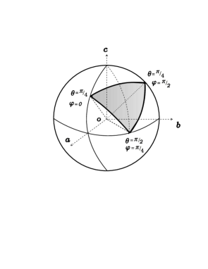
Figure 1: The intersection of an $r=constant$ surface with the space of orbits for three particles in the Cartesian frame of the distances is a spherical triangle, the boundaries of which are arcs of great circles.

The domain of the polar and azimuthal angles $\theta$ and $\varphi$ defined in the Cartesian system spanned by the coordinate lines ${a_{i}}$ is restricted first by the positivity of $a_{i}$:

$$0\leq\theta\leq{\frac{\pi}{2}}\ ,\qquad 0\leq\varphi\leq{\frac{\pi}{2}}\ ,$$ (1)

second by the triangle inequality:

$$\mid\sin\varphi-\cos\varphi\mid\leq\cot\theta\leq\sin\varphi+\cos\varphi\ .$$ (2)

Therefore the reduced space can be imagined like a diverging beam of rays starting from the origin, with a triangular section, as can be seen on Fig 1. The boundaries of the admissible domain of the reduced space are defined by the equalities in Eq. (2) as planes passing through the origin. In consequence each constant radius section of the reduced space is bounded by arcs of great circles. The origin $O$ corresponds to the unphysical situation of all three particles in the same location while the planar boundaries to the situation of the three particles on a line. The edges of the beam (the intersection of two plane boundaries) are again unphysical: there the positions of two of the three particles coincide. On all boundaries of the space of orbits the inertia matrix has vanishing determinant, consequently the metric (32) of I is ill-defined there. On the other hand the scalar curvature is well behaved in the line configurations, suggesting that the boundary planes (including the edges but not the origin $O$) are merely coordinate singularities. Topologically the region inside the boundaries is the quotient space $R^{9}/E(3)$, where $E(3)=R^{3}\rtimes SO(3)$ and is homeomorphic to half of $R^{3}$. The boundary is homeomorphic to $R^{2}$ [4].

The special situation of the restricted three-body problem, with a lighter third body orbiting about the other two heavier, whose separation is not changing is confined within intersections of the space of orbits (the ”beam”) with one of the planes $a_{i}=const$.

As physically the line configurations are no more special then others, our description has to allow the geodesics to reach and to leave the boundaries. We then require that a geodesic reaching the boundary at some instant $t_{0}$ should not leave the admissible domain of the $\{a_{i}\}$ space, by imposing the following boundary conditions:

$${\bf\dot{a}}_{\perp}(t_{0})=0\ ,$$ (3)

$${\bf\ddot{a}}_{\perp}(t_{0})<0\ .$$ (4)

Here ${\bf\dot{a}}_{\perp}$ and ${\bf\ddot{a}}_{\perp}$ represent the projections perpendicular to the boundary of the first and second derivatives of the position vector ${\bf a}=(a,b,c)$ with respect to the geodesic parameter. The perpendicularity is meant in an Euclidean sense, by projecting ${\bf\dot{a}}$ and ${\bf\ddot{a}}$ to the outer normal to the boundary surface.

Proof of the boundary conditions:

It is well known that the motion of a three body system with vanishing angular momentum ${\bf L}=\sum_{A}{\bf L}_{A}=0$ is confined to a plane [7]. By using Cartesian coordinates $(x,\ y,\ z)$ we choose $z_{A}=0=\dot{z}_{A}$ and then the constraints $\sum_{A}{\bf P}_{Az}=\sum_{A}{\bf L}_{Ax}=\sum_{A}{\bf L}_{Ay}=0$ are trivially satisfied. The distances ${a_{i}}$ are given as:

$$a^{2}=(x_{2}-x_{3})^{2}+(y_{2}-y_{3})^{2}\ ,$$

$$b^{2}=(x_{3}-x_{1})^{2}+(y_{3}-y_{1})^{2}\ ,$$

$$c^{2}=(x_{1}-x_{2})^{2}+(y_{1}-y_{2})^{2}\ .$$ (5)

As parameter of the geodesic the time can be chosen. The time derivative of (5) gives $\{\dot{a}_{i}\}$

$$a\dot{a}=(x_{2}-x_{3})(\dot{x}_{2}-\dot{x}_{3})+(y_{2}-y_{3})(\dot{y}_{2}-\dot{y}_{3})\ ,$$

$$b\dot{b}=(x_{3}-x_{1})(\dot{x}_{3}-\dot{x}_{1})+(y_{3}-y_{1})(\dot{y}_{3}-\dot{y}_{1})\ ,$$

$$c\dot{c}=(x_{1}-x_{2})(\dot{x}_{1}-\dot{x}_{2})+(y_{1}-y_{2})(\dot{y}_{1}-\dot{y}_{2})\ .$$ (6)

From among the ”velocities” $\dot{x}_{1},\ \dot{x}_{2},\ \dot{x}_{3},\ \dot{y}_{1},\ \dot{y}_{2},\ \dot{y}_{3}$ only three are independent due to the remaining constraints $\sum_{A}{\bf P}_{Ax}=\sum_{A}{\bf P}_{Ay}=\sum_{A}{\bf L}_{Az}=0$. However for the purpose of the proof it is not necessary to make this manifest. We just comment that in general $\{\dot{a}_{i}\}$ depend on three arbitrary velocities and in the majority of cases they are independent. A notable exception is given by the collinear configurations, as will be seen later. In the computation of the second derivatives we employ that the motions are free, $\ddot{x}_{A}=\ddot{y}_{A}=0$:

$$a\ddot{a}+{\dot{a}}^{2}=(\dot{x}_{2}-\dot{x}_{3})^{2}+(\dot{y}_{2}-\dot{y}_{3})^{2}\ ,$$

$$b\ddot{b}+{\dot{b}}^{2}=(\dot{x}_{3}-\dot{x}_{1})^{2}+(\dot{y}_{3}-\dot{y}_{1})^{2}\ ,$$

$$c\ddot{c}+{\dot{c}}^{2}=(\dot{x}_{1}-\dot{x}_{2})^{2}+(\dot{y}_{1}-\dot{y}_{2})^{2}\ .$$ (7)

Then we study the collinear configurations. By a rotation in the $xy$ plane, it can be achieved that the collinearity arises on the $x$-axis. We label the particles as $(3,\ 1,\ 2)$ in order of increasing $x$-coordinate. In this way $x_{3}-x_{1}=-b,\ x_{1}-x_{2}=-c,\ x_{2}-x_{3}=a$ and the boundary is expressed by $a=b+c$, with the outer normal ${\bf n}=(1,\ -1,\ -1)$. The system (6) becomes

$$\dot{a}=(\dot{x}_{2}-\dot{x}_{3})\ ,\quad\dot{b}=-(\dot{x}_{3}-\dot{x}_{1})\ ,\quad\dot{c}=-(\dot{x}_{1}-\dot{x}_{2})\ .$$ (8)

It is immediate to show ${\bf\dot{a}}_{\perp}={\bf\dot{a}}\cdot{\bf n}=0$. Employing Eqs. (8), the system (7) can be written in the form

$$(b+c)\ddot{a}=(\dot{y}_{2}-\dot{y}_{3})^{2}\ ,\quad b\ddot{b}=(\dot{y}_{3}-\dot{y}_{1})^{2}\ ,\quad c\ddot{c}=(\dot{y}_{1}-\dot{y}_{2})^{2}\ .$$ (9)

By simple algebra we find then

$${\bf\ddot{a}}_{\perp}={\bf\ddot{a}}\cdot{\bf n}=-\frac{[b(\dot{y}_{1}-\dot{y}_{2})+c(\dot{y}_{3}-\dot{y}_{1})]^{2}}{bc(b+c)}<0$$ (10)

which completes the proof of the boundary conditions, Eqs. (3)-(4).

Q.E.D.

3 The curvature scalar for three particles

In this section we work out the expression for the curvature scalar (given in I in terms of the principal moments of inertia) for the particular case of three particles. For this purpose first we write the principal moments of inertia in terms of the relative separations.

By choosing the positions of the three particles in some initial coordinate system (Fig. 2) originating in the center of mass as $\mathop{x}\limits_{\circ}{}^{1a}=(x,0,0),\ \mathop{x}\limits_{\circ}{}^{2a}=(\xi,y,0)$ and $\mathop{x}\limits_{\circ}{}^{3a}=(-x_{3},-y_{3},0)$, the $x_{3}$ and $y_{3}$ coordinates are determined by the condition $\sum_{A}m_{A}\mathop{x}\limits_{\circ}{}^{Aa}=0$:

$$x_{3}={\frac{m_{1}x+m_{2}\xi}{m_{3}}}\qquad y_{3}={\frac{m_{2}}{m_{3}}}y\ .$$ (11)

The remaining three coordinates $(x,\xi,y)$ are related to the relative distances as:

$$m_{3}^{2}a^{2}=\left[m_{1}x+(m_{2}+m_{3})\xi\right]^{2}+(m_{2}+m_{3})^{2}y^{2}$$

$$m_{3}^{2}b^{2}=\left[(m_{1}+m_{3})x+m_{2}\xi\right]^{2}+m_{2}^{2}y^{2}$$

$$c^{2}=x^{2}+y^{2}+\xi^{2}-2x\xi\ .$$ (12)

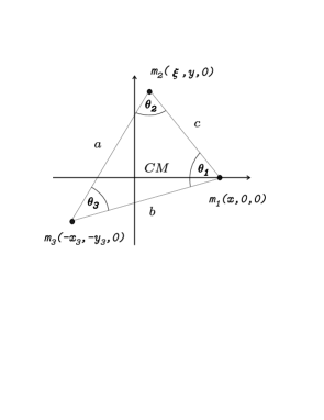
Figure 2: The three particles in the center of mass frame.

We introduce the positive quantities $A,W$ and $Z$, depending only on relative distances and with the dimensions of moments of inertia, as follows:

$$W={\frac{m_{1}m_{2}c^{2}+m_{2}m_{3}a^{2}+m_{3}m_{1}b^{2}}{2M}}\ ,\qquad A={\frac{m_{2}m_{3}}{m_{2}+m_{3}}}a^{2}\ ,$$

$$Z^{2}={\frac{m_{1}m_{2}m_{3}}{4M}}(a+b+c)(a+b-c)(a-b+c)(-a+b+c)\ .$$ (13)

Heron’s formula relates the quantity $Z$ to the area ${\cal A}$ of the triangle: $Z=2{\cal A}\sqrt{m_{1}m_{2}m_{3}/M}$. From Eqs. (12) and Eqs. (13) a useful relation is found:

$$\sum_{A}m_{A}\mathop{x}\limits_{\circ}{}^{Ac}\mathop{x}\limits_{\circ}{}^{Ad}\delta_{cd}=2W$$ (14)

A computation employing the definition of the inertia tensor in the center of mass frame (Eq. (21) of I) and Eqs. (12), (13) and (14) yields the expression of the tensor of inertia in terms of distances:

$$\mathop{I}\limits_{\circ}{}_{gh}=\!\!\left(\!\!\begin{array}[]{lll}I_{11}&-\sqrt{I_{11}(2W-I_{11})-Z^{2}}&0\\ -\sqrt{I_{11}(2W-I_{11})-Z^{2}}&2W-I_{11}&0\\ 0&0&2W\end{array}\!\!\right)\!\!,$$ (15)

where

$$I_{11}={\frac{Z^{2}}{(2W-A)}}\ .$$ (16)

From here we find the principal moments of inertia:

$$I_{1,2}=W\pm\sqrt{W^{2}-Z^{2}}\ ,\qquad I_{3}=2W\ .$$ (17)

They contain the relative distances and the masses in a symmetric fashion ($I_{11}$, which is the only term containing the non-symmetric expression $A$, dropped out from their expression). By insertion of the principal moments of inertia in Eq. (43) of I we have an independent check of Eq. (14).

The curvature scalar of the reduced space given by Eq. (51) of I, written in terms of the distances takes the remarkably simple expression:

$$R={\frac{3}{W}}\ .$$ (18)

As expected from the argumentation in I, the curvature scalar is well behaved even in the case of all three particles in a line. This suggests that in the line configurations a coordinate singularity occurs. By contrast, the unphysical situation of all particles in a point represents a true curvature singularity, as $W$ vanishes there.

4 Metric properties

In order to find the metric in the space of orbits in terms of the distances $a_{i}$ we start from the degenerated metric (32) of I. Then we pass to the basis associated with the coordinates $(y^{i},\ \alpha_{j},\ x^{k}),$ where $y^{i}=(x,\ \xi,\ y)$. The relevant part of the transformation matrix is given by

$$\frac{\partial\mathop{x}\limits_{\circ}{}^{Ai}}{\partial y^{j}}=\left(\delta_{1}^{A}-\frac{m_{1}}{m_{3}}\delta_{3}^{A}\right)\delta_{1}^{i}\delta_{j}^{1}+\left(\delta_{2}^{A}-\frac{m_{2}}{m_{3}}\delta_{3}^{A}\right)\left(\delta_{1}^{i}\delta_{j}^{2}+\delta_{2}^{i}\delta_{j}^{3}\right)\ .$$ (19)

The $3\times 3$ block with the basis in the 1-forms $dy^{i}$ then is transformed to the basis $da_{i}$ through the relations (12). Finally we get:

$$G^{ij}=\left(\matrix{\displaystyle{\frac{m_{2}+m_{3}}{m_{2}m_{3}}}&\displaystyle{\frac{a^{2}+b^{2}-c^{2}}{2m_{3}ab}}&\displaystyle{\frac{a^{2}-b^{2}+c^{2}}{2m_{2}ac}}\cr&&\cr\displaystyle{\frac{a^{2}+b^{2}-c^{2}}{2m_{3}ab}}&\displaystyle{\frac{m_{1}+m_{3}}{m_{1}m_{3}}}&\displaystyle{\frac{-a^{2}+b^{2}+c^{2}}{2m_{1}bc}}\cr&&\cr\displaystyle{\frac{a^{2}-b^{2}+c^{2}}{2m_{2}ac}}&\displaystyle{\frac{-a^{2}+b^{2}+c^{2}}{2m_{1}bc}}&\displaystyle{\frac{m_{1}+m_{2}}{m_{1}m_{2}}}}\right)\ .$$ (20)

The covariant form of the metric has a more complicated expression. Eq. (20) is the induced metric in the space of orbits. It is not surprising, that $G^{ij}$ is manifestly symmetric in both masses and distances, because the overall translational and rotational degrees of freedom have been suppressed.

Remarkably, the metric $G^{ij}$ has a conformal symmetry. Indeed, (20) is unchanged under multiplying all distances with the same factor, thus $G^{ij}$ is homogeneous of degree zero in $a_{i}$. The Euler theorem for homogeneous functions gives then $\sum_{k}G_{\ \,k}^{ij}a_{k}=0$ for any point of the reduced space with coordinates $a_{i}$. Then the vector

$$K^{i}=a_{i}=(a,b,c)$$ (21)

is a conformal Killing vector, generating a homothetic motion:

$${\ell}_{K}\ G^{ij}=-2G^{ij}$$ (22)

The norm and covariant components of this conformal Killing vector can be expressed in terms of the previously introduced quantity $W$:

$$K=\sqrt{2W}\ ,\qquad K_{i}={\frac{1}{M}}(m_{2}m_{3}a,\ m_{1}m_{3}b,\ m_{1}m_{2}c)=\nabla_{i}W\ .$$ (23)

Here $\nabla$ denotes the connection compatible with the metric $G$.

The distance in the metric $G_{ij}$ of any point from the origin is the length of the corresponding conformal Killing vector (23). Thus the curvature scalar (18) is just 6 divided by the square of this distance.

Whenever one has a metric $G^{ij}$ with a conformal symmetry, by an appropriate rescaling a new metric $\bar{G}^{ij}=\Omega^{2}G^{ij}$ can be found which has the property, that the conformal Killing vector of $G^{ij}$ is a true Killing vector of the metric $\bar{G}^{ij}$. In our case the scaling function was found to be $\Omega^{2}=a^{2}+b^{2}+c^{2}=r^{2}$. Choosing an adapted coordinate system the metric $\bar{G}^{ij}$ does not depend on $r$. Such a coordinate system is given by $(ln\ r,\ \theta,\ \varphi)$ in which the conformal Killing vector of $G^{ij}$ takes the simple form $K^{i}=(1,0,0)$. Thus the metric $G^{ij}$ is expected to have the form:

$$G^{ij}=\frac{1}{r^{2}}\cdot\bar{G}^{ij}(angles)\ .$$ (24)

Unfortunately the attempts to write the metric in terms of the radial coordinate $r$, supplemented by any two angular coordinates, have resulted in less symmetric forms.

In the search for angular variables which give a reasonably simple form of the metric, we have found a convenient (but redundant) set given by the sines

$$s_{i}=\sin\theta_{i}$$ (25)

of the three angles $\theta_{i}$ (Fig.2.). The condition $\theta_{1}+\theta_{2}+\theta_{3}=\pi$ constrains the variables $s_{i}$ as follows:

$$s_{1}^{2}+s_{2}^{2}-s_{3}^{2}=2s_{1}s_{2}\sqrt{1-s_{3}^{2}}$$ (26)

and all of its cyclic permutations. The square of Eq. (26) yields a symmetric form of this constraint:

$$(s_{1}+s_{2}+s_{3})(s_{1}+s_{2}-s_{3})(s_{1}-s_{2}+s_{3})(s_{2}+s_{3}-s_{1})=4s_{1}^{2}s_{2}^{2}s_{3}^{2}\ .$$ (27)

From the sine theorem we find that the relative separations are related to the redundant variables $s_{i}$ as:

$$a_{i}=\frac{r}{S}s_{i}\ ,$$ (28)

where $S^{2}=s_{1}^{2}+s_{2}^{2}+s_{3}^{2}$. By multiplying Eq. (27) with $(r/S)^{6}$ we find $S^{2}$ in terms of the distances:

$$S^{2}=\frac{Mr^{2}Z^{2}}{m_{1}m_{2}m_{3}a^{2}b^{2}c^{2}}\ .$$ (29)

We also introduce the quantity

$$\sigma^{2}=\frac{2MWS^{2}}{r^{2}}=m_{1}m_{2}s_{3}^{2}+m_{2}m_{3}s_{1}^{2}+m_{3}m_{1}s_{2}^{2}=\frac{2M^{2}WZ^{2}}{m_{1}m_{2}m_{3}a^{2}b^{2}c^{2}}\ ,$$ (30)

which depends only on the angular variables $s_{i}$ as can be seen from the second form given in Eq. (30). The third form arises by inserting Eq. (29) in the first form and similarly to Eq. (29) is useful in rewriting the angular expressions in terms of the distances.

By multiplying Eq. (26) with $(r/S)^{2}$ the following relation emerges:

$$\sqrt{1-s_{3}^{2}}=\frac{a^{2}+b^{2}-c^{2}}{2ab}\ .$$ (31)

Similar equations follow for the cyclic permutations. Therefore the contravariant metric expressed in these new angle variables, while keeping the basis of the metric in the 1-forms ${da_{i}}$, takes the concise form:

$$G^{ij}=\frac{\left(M-m_{j}\right)m_{j}}{m_{1}m_{2}m_{3}}\delta^{ij}+\sum\limits_{k}\frac{\sqrt{1-s_{k}^{2}}}{m_{k}}\mu^{ijk}\ .$$ (32)

Here $\mu^{ijk}$ is the ”square” of the symbol $\epsilon^{ijk}$, zero for any pair of coinciding indices and taking the value $1$ otherwise and no summation over $j$ applies.

The concise form (32) of the metric allows us to study its signature. First we remark that all three diagonal elements of $G^{ij}$ (the first term in (32)) are positive. Also all three sub-determinants of the diagonal elements have similar forms, for example the sub-determinant of $G^{11}$ is

$$\frac{s_{3}^{2}}{m_{3}^{2}}+\frac{M}{m_{1}m_{2}m_{3}}\ ,$$ (33)

and are also positive. Finally the determinant $1/G$ of $G^{ij}$,

$$G^{-1}=\frac{M\sigma^{2}}{m_{1}^{2}m_{2}^{2}m_{3}^{2}}$$ (34)

is positive except in the singular configuration of particles in a line, where $\sigma^{2}$ is zero. Therefore we are in the position to conclude that the metric is positive definite, modulo the boundaries where it diverges.

Direct computation of the curvature scalar from the metric yields (18) once again, which in terms of the angular variables and $r$ takes the form:

$$R=\frac{6MS^{2}}{\sigma^{2}r^{2}}\ .$$ (35)

The Ricci tensor can be expressed in terms of the curvature scalar:

$$R_{ij}=R\frac{m_{1}m_{2}m_{3}}{2\sigma^{2}}\left[\delta_{ij}-\sum\limits_{k}\sqrt{1-s_{k}^{2}}\ \mu_{ijk}\right]\ .$$ (36)

As in three dimensions the Weyl tensor vanishes, the Riemann tensor is determined completely by the Ricci tensor, the curvature scalar and the metric:

$$R_{ijkl}=2G_{i[k}R_{l]j}-2G_{j[k}R_{l]i}-RG_{i[k}G_{l]j}\ .$$ (37)

Again we write the result of the computation in terms of the curvature scalar:

$$R_{ijkl}=R\frac{m_{1}^{2}m_{2}^{2}m_{3}^{2}}{2\sigma^{4}}\sum\limits_{a}\epsilon_{ija}s_{a}\sum\limits_{b}\epsilon_{klb}s_{b}\ .$$ (38)

All multiplying factors of $R$ in $R_{ijkl}$ and $R_{ij}$ depend only on the angular variables, thus these tensors depend on $r$ only through $R$.

Next we study the behavior of the curvature in the line configurations. Though the curvature scalar is undetermined in the form (35), it is clearly nonsingular when written in terms of the distances (18), as already remarked. From Eq. (38) we compute the Kretschmann scalar and find that it is nonsingular either:

$$R_{ijkl}R^{ijkl}=R^{2}\ .$$ (39)

From Eq. (37) an algebraic relation can be deduced between these scalars

$$R_{ijkl}R^{ijkl}-4R_{ij}R^{ij}+R^{2}=0\ ,$$ (40)

which gives

$$R_{ij}R^{ij}=\frac{R^{2}}{2}\ .$$ (41)

In fact in three dimensions there are only three independent scalars which can be formed from the Riemann tensor and the metric. These can be given either as

$$R\ ,\qquad R_{ij}R^{ij}\ ,\qquad\frac{Det(R)}{Det(G)}$$ (42)

or as the roots of the secular equation $Det(R_{ij}-\lambda G_{ij})=0$ [8]. To complete the first set (42) we compute

$$\frac{Det(R)}{Det(G)}=0\ ,$$ (43)

while the secular equation will be dealt with in the next section.

Finally we remark that in three dimensions the vanishing of the tensor

$$R_{abc}=\nabla_{c}R_{ab}-\nabla_{b}R_{ac}+\frac{1}{4}(G_{ac}\nabla_{b}R-G_{ab}\nabla_{c}R)$$ (44)

is equivalent with the conformal flatness of the metric [9]. The computation gives $R_{abc}=0$, therefore the metric is conformally flat:

$$G^{ab}=\Phi^{2}\eta^{ab}\ .$$ (45)

Here $\eta_{ab}$ denotes a flat metric. The conformal factor can be determined by solving the differential equation which arises from the comparison of the expression (18) with the formula [10] relating the curvature scalars of the metrics $G^{ab}$ and $\eta^{ab}$ (the curvature of the latter being zero):

$$R=\frac{2G^{ab}\nabla_{a}\nabla_{b}\Phi^{2}}{\Phi^{2}}-\frac{3G^{ab}\nabla_{a}\Phi^{2}\nabla_{b}\Phi^{2}}{2\Phi^{4}}\ .$$ (46)

It is easy to prove that

$$\Phi^{2}=\alpha W\ ,$$ (47)

$\alpha$ arbitrary constant, solves the differential equation, by employing Eqs. (23) and the relation $\nabla_{a}K^{a}=3$, which stems out from the conformal Killing equation (22).

A coordinate system $\{w_{i}\}$, related to the Jacobi coordinates, frequently used [6] in molecular dynamics, has the advantageous property that $\eta^{ab}=diag(1,1,1)$. The price one has to pay in using such coordinates is that they depend on the distances in a nonsymmetric fashion:

$$w_{1}=2(B-W)\ ,\quad w_{2}=2\sqrt{2BW-B^{2}-Z^{2}}\ ,\quad w_{3}=2Z\ ,$$ (48)

where the notation $B=m_{1}m_{3}b^{2}/(m_{1}+m_{3})$ was introduced. In the coordinates $\{w_{i}\}$ the constant in the conformal factor (47) is $\alpha=8$.

5 Sectional curvatures

In this section we study the eigenvalue problem of the Ricci tensor (36):

$$R_{\ j}^{i}\mathop{n}\limits_{\alpha}{}^{j}=\mathop{\rho}\limits_{\alpha}{}\mathop{n}\limits_{\alpha}{}^{i}\ .$$ (49)

The eigenvalues $\mathop{\rho}\limits_{\alpha}{}$ are $0$ and a double root equal to $R/2$. All eigenvalues are well behaved for the configuration of particles in a line. The conformal Killing vector $K^{i}$ (21) is the eigenvector corresponding to the zero eigenvalue. A two-dimensional subspace spanned by the vectors:

$$X_{(1)}^{i}=\left(0,\ c/m_{3},\ -b/m_{2}\right)$$

$$X_{(2)}^{i}=\left(-c/m_{3},\ 0,\ a/m_{1}\right)$$

$$X_{(3)}^{i}=\left(b/m_{2},\ -a/m_{1},0\right)$$ (50)

corresponds to the degenerate eigenvalue $R/2$. Any two of these vectors are linearly independent, but not orthogonal to each other. From the general theory of symmetric matrices we know that the two-dimensional space spanned by $X_{(\nu)}^{i}$ is orthogonal to $K^{i}$. A compact notation for the eigenvectors is:

$$K^{i}=a_{i}\ ,\qquad X_{(\nu)}^{i}=\sum_{j}\epsilon_{\nu ij}{\frac{a_{j}}{m_{j}}}\$$ (51)

and for a dual set of the eigenvectors:

$$K_{i}={\frac{1}{2M}}\sum_{j,k}\mu_{ijk}a_{i}m_{j}m_{k}$$

$$Y_{i}^{(\nu)}=-\sum_{j}\mu_{\nu ij}m_{j}a_{i}a_{\nu}+\delta_{i}^{\nu}\sum_{jk}\mu_{ijk}m_{j}a_{k}^{2}\ .$$ (52)

Each of the one-forms $Y_{i}^{(\nu)}$ is the dual of some vector $Y_{(\nu)}^{i}$, orthogonal to both $K^{i}$ and $X_{(\nu)}^{i}$.

It is immediate to check that the set of vectors $Y_{(\nu)}^{i}$ and $K^{i}$ are surface orthogonal, as they satisfy the relations:

$$K_{i,j}K_{k}\epsilon^{ijk}=0\ ,\qquad Y_{i,j}^{(\nu)}Y_{k}^{(\nu)}\epsilon^{ijk}=0\ .$$ (53)

We proceed to find these privileged surfaces. It follows from (23) that the ellipsoids

$$F\equiv W-const=0\ ,$$ (54)

are the surfaces orthogonal to $K^{i}$. Then the surfaces $f^{(\nu)}=0$ orthogonal to the vectors $Y_{(\nu)}^{i}$ can be determined by imposing the proportionality of their gradients with $Y_{i}^{(\nu)}$:

$$Y_{i}^{(\nu)}=\lambda^{(\nu)}\nabla_{i}f^{(\nu)}\ ,$$ (55)

by some undetermined factor $\lambda^{(\nu)}$. The detailed derivation is given below for the surface orthogonal to $Y_{(3)}^{i}$. We look for this surface in the form

$$f^{(3)}\equiv\Theta(c)-\Phi(a,b)\ .$$ (56)

Comparing the expressions of $Y_{i}^{(3)}$ from (52) and (55) we find three equations to determine the unknown functions $\Theta(c),$ $\Phi(a,b)$ and $\lambda^{(3)}$, which are:

$$\lambda^{(3)}\Theta_{,3}=m_{1}b^{2}+m_{2}a^{2}$$

$$\lambda^{(3)}\Phi_{,1}=m_{2}ac$$ (57)

$$\lambda^{(3)}\Phi_{,2}=m_{1}bc\ ,$$

By inserting $\lambda^{(3)}$ expressed from the first equation into the rest of the system (57), the remaining equations can be brought into the form

$$\frac{c}{2}\frac{d\Theta}{dc}=\alpha=(m_{1}b^{2}+m_{2}a^{2})\frac{d\Phi}{d\left(m_{1}b^{2}+m_{2}a^{2}\right)}\ ,$$ (58)

which has the immediate solution $\Theta=\alpha\ln(\gamma c^{2})$ and $\Phi=\alpha\ln[\beta(m_{1}b^{2}+m_{2}a^{2})].$ Here $\alpha,\ \beta$ and $\gamma$ are constants. Thus the equation of the surface orthogonal to the vector $Y_{(3)}^{i}$ is given by:

$$f^{(3)}\equiv\alpha\ln\Bigl{[}\frac{\gamma c^{2}}{\beta(m_{1}b^{2}+m_{2}a^{2})}\Bigr{]}=0\ ,$$ (59)

or equivalently as

$$F^{(3)}\equiv m_{1}b^{2}+m_{2}a^{2}-const\cdot c^{2}=0\ ,$$ (60)

Similar equations with cyclically permuted quantities define the surfaces to which the other two vectors $Y_{(\nu)}^{i}$ are orthogonal. These surfaces are cones with the tips in the origin and they have elliptical sections.

Next we derive the sectional curvatures of the privileged sections $F$ and $F^{(\nu)}$. We pick up an independent set of eigenvectors $\mathop{n}\limits_{\alpha}{}^{i}$ by normalizing $K^{i}$ and any two of the three vectors $Y_{(3)}^{i}$. For each of these surfaces we define the Riemann tensors ${}^{(2)}\hskip-2.84544pt\mathop{R}\limits_{\alpha}{}_{\ bcd}^{a}$ like in Eq. (46) of I. We also define the projector operators $\mathop{P}\limits_{\alpha}{}_{b}^{a}$ and the extrinsic curvatures $\mathop{K}\limits_{\alpha}{}_{ab}$ for the sections:

$$\mathop{P}\limits_{\alpha}{}_{b}^{a}=\delta_{b}^{a}-\mathop{n}\limits_{\alpha}{}^{a}\mathop{n}\limits_{\alpha}{}_{b}\ ,\qquad\mathop{K}\limits_{\alpha}{}_{ab}=P_{a}^{c}P_{b}^{d}\nabla_{c}\mathop{n}\limits_{\alpha}{}_{d}\ .$$ (61)

The Gauss equation connects the curvature tensor and extrinsic curvature of the sections to the curvature tensor of the space of distances:

$${}^{(2)}\hskip-2.84544pt\mathop{R}\limits_{\alpha}{}_{abcd}=\mathop{P}\limits_{\alpha}{}_{a}^{e}\mathop{P}\limits_{\alpha}{}_{b}^{f}\mathop{P}\limits_{\alpha}{}_{c}^{g}\mathop{P}\limits_{\alpha}{}_{d}^{h}R_{efgh}+2\mathop{K}\limits_{\alpha}{}_{a[c}\mathop{K}\limits_{\alpha}{}_{d]b}\ .$$ (62)

A double contraction with the induced metric on the sections $G^{ab}-\mathop{n}\limits_{\alpha}{}^{a}\mathop{n}\limits_{\alpha}{}^{b}$ gives the equations for the sectional curvatures:

$${}^{(2)}\hskip-2.84544pt\mathop{R}\limits_{\alpha}{}=R-2\mathop{\rho}\limits_{\alpha}{}+(\mathop{K}\limits_{\alpha}{}_{\ a}^{a})^{2}-\mathop{K}\limits_{\alpha}{}_{ab}\mathop{K}\limits_{\alpha}{}^{ab}\ .$$ (63)

Here we have employed that $\mathop{n}\limits_{\alpha}{}^{a}$ is eigenvector of the Ricci tensor, Eq. (49).

Straightforward computation based on the above prescription has shown that the sectional curvature of the conical surfaces $F^{(\nu)}=0$ vanishes.

For the ellipsoid surfaces with the normal $n^{i}=K^{i}/\sqrt{2W}$ the extrinsic curvature is found readily from the equation of the homothetic motion (22). In terms of $n^{i}$ the covariant form of this equation is:

$$\nabla_{i}n_{j}+\nabla_{j}n_{i}=\sqrt{\frac{2}{W}}\left(G_{ij}-n_{i}n_{j}\right)\ .$$ (64)

Contracting twice with the projectors to the ellipsoid surface, the desired result emerges:

$$K_{ij}={\frac{1}{\sqrt{2W}}}\left(G_{ij}-n_{i}n_{j}\right)\ .$$ (65)

A simple computation then yields

$$(\mathop{K}\limits_{\alpha}{}_{\ a}^{a})^{2}-\mathop{K}\limits_{\alpha}{}_{ab}\mathop{K}\limits_{\alpha}{}^{ab}={\frac{1}{W}}$$ (66)

and from (63), the sectional curvature of the ellipsoid surface $F=0$ is found:

$${}^{(2)}R={\frac{4}{W}}={\frac{4}{3}}R\ .$$ (67)

This is constant on the ellipsoids, therefore in the metric $G_{ij}$ the $F=0$ surfaces are spheres.

6 Geodesic motions

The equation for the homothetic motion (22) carries even more information. A contraction of its covariant form with $K^{j}$ gives:

$$K^{j}\nabla_{j}K_{i}+{\frac{1}{2}}(K_{j}K^{j})_{,i}=2K_{i}\ .$$ (68)

The second term is simply $K_{i}$ as can be seen from (23). Thus the integral curves of the conformal Killing vector field $K^{i}$ are geodesics:

$$K^{j}\nabla_{j}K_{i}=K_{i}\ .$$ (69)

We recall that $K^{i}\partial/\partial x^{i}=\partial/\partial\ln r.$ Therefore $\ln r$ is not an affine parameter, however it is easy to check that $pr+q$ is, if $p$ and $q$ are constants.

Eq. (69) says that the motions along radial lines of the reduced space are geodesics. Therefore the boundaries of the reduced space (Fig. 1) are geodesic planes in the sense that they are spanned by geodesics passing through the origin. The privileged conical surfaces $F^{(\nu)}=0$ are geodesic surfaces in the same sense.

The ellipsoid sections $F=0$ are not geodesic surfaces. To see this, we compute the Gaussian curvature ${\cal K}$ of a geodesic surface whose tangent space in each point is spanned by any two of the (non-orthogonal) eigenvectors $Y_{(\mu)}^{i}$ by means of [9]

$$\ {\cal K}=\frac{R_{hijk}Y_{(\mu)}^{h}Y_{(\nu)}^{i}Y_{(\mu)}^{j}Y_{(\nu)}^{k}}{\left(G_{nl}G_{mp}-G_{lp}G_{mn}\right)Y_{(\mu)}^{l}Y_{(\nu)}^{m}Y_{(\mu)}^{n}Y_{(\nu)}^{p}}\ .$$ (70)

We have found $\ {\cal K}=R/2$. Since the Gaussian curvature is half of the curvature scalar, the latter would be ${}^{(2)}R_{geod}=2{\cal K}=R$ for a geodesic surface with tangents $Y_{(\mu)}^{i}$. This is different from the scalar curvature (67) of the ellipsoid sections with the same tangents. Therefore the ellipsoid sections cannot be geodesic surfaces (in each point they have common tangents with different geodesic surfaces).

In order to have the generic geodesic motions

$$\frac{d^{2}a_{i}}{d\lambda^{2}}+\Gamma_{jk}^{i}\frac{da_{j}}{d\lambda}\frac{da_{k}}{d\lambda}=0\ ,$$ (71)

we need the Christoffel symbols $\Gamma_{jk}^{i}$ of the space of orbits. They are given as

$$\Gamma_{jk}^{i}=\frac{m_{1}m_{2}m_{3}}{16M^{3}W^{2}Z^{2}}m_{i}^{2}\Biggl{\{}\mu_{ijk}a_{i}a_{j}a_{k}\Lambda_{ijk}\Lambda_{ikj}$$

$$-\delta_{jk}a_{i}a_{j}^{2}\sum_{p}\mu_{ijp}\Lambda_{ipj}^{2}-\delta_{jk}\delta_{ij}\frac{1}{a_{i}}\Bigl{(}\sum_{p,q}\epsilon_{ipq}\Xi_{pq}\Bigr{)}^{2}$$

$$+\left[\delta_{ik}a_{j}\sum_{p}\mu_{ijp}\Lambda_{ipj}(\Xi_{pj}-\Xi_{jp})+(j\leftrightarrow k)\right]\Biggr{\}}\ .$$ (72)

In the above formula and the forthcoming ones all summations are indicated explicitly. The coefficients $\Lambda_{ijk}$ and $\Xi_{ij}$ have the expressions:

$$\Lambda_{ijk}=\Bigl{(}\sum_{r}a_{r}^{2}-2a_{i}^{2}\Bigr{)}m_{j}+2a_{j}^{2}m_{k}$$ (73)

$$\Xi_{ij}=\Bigl{(}\sum_{r}a_{r}^{2}-2a_{i}^{2}\Bigr{)}a_{i}^{2}m_{j}$$ (74)

We note here that in the $\{a_{i}\}$ coordinates $\Gamma_{jk}^{i}$ diverges on the boundaries. The geodesic equations (71), supplemented by the boundary conditions (3) and (4) represent the equations of motion for the three-body problem with vanishing constants of motion, constant potential case, in terms of relative separations.

We seek for solutions of the geodesic equation in the following form

$$\lambda=t\ ,\qquad a_{i}(t)=\sqrt{A_{i}t^{2}+B_{i}t+C_{i}}\ .$$ (75)

These characterize the uniform velocity, straight line motions of the particles in the physical space. For such motions the vanishing of the energy is assured by a proper choice of the constant $V$. The coefficients $A_{i},B_{i}$ and $C_{i}$ are functions of the relative positions ${\bf r}_{jk}={\bf r}_{j}-{\bf r}_{k}$ and relative velocities ${\bf\dot{r}}_{jk}$ of the three particles at some initial time:

$$A_{i}\!=\!\frac{1}{2}\sum_{j,k}\!\mu_{ijk}{\bf\dot{r}}_{jk}^{2}\ ,\quad B_{i}\!=\!\sum_{j,k}\mu_{ijk}{\bf r}_{jk}\!\cdot\!{\bf\dot{r}}_{jk}\ ,\quad C_{i}\!=\!\frac{1}{2}\sum_{j,k}\!\mu_{ijk}{\bf r}_{jk}^{2}\ .$$ (76)

Therefore $A_{i}=0$ and $C_{i}=0$ both imply $B_{i}=0$ too.

It is straightforward to check that particular cases of the motions (75) fulfill the geodesic equation (71). In the case $A_{i}=0$ the geodesic equations are trivially satisfied, this choice of the constants corresponding to no motion at all in the space of orbits. When $C_{i}=0$, then $a_{i}(t)=\sqrt{A_{i}}t$ are geodesics passing through the origin, with affine parameter $t$. These are the motions with tangents $K^{i}$, the affine parameter $t$ being linearly related to the radial coordinate $r$. The same type of motions $a_{i}(t)=\sqrt{A_{i}}t+\sqrt{C_{i}}$ emerge also for the choice $B_{i}=2\sqrt{A_{i}C_{i}}$. In this latter case Eqs. (76) imply $A_{i}=\varphi C_{i}$ therefore ${\bf\dot{r}}_{jk}=\varphi{\bf r}_{jk}$. The special case of a pure expansion motion (a similarity transformation of the triangle of Fig. 2) is included here as the particular case with ${\bf\dot{r}}_{i}=\varphi{\bf r}_{i}$.

Those motions (75) which do not violate the constraints ${\bf P}=0$ and ${\bf L}=0$ are expected to be geodesics with affine parameter $t$. The fact that not all motions (75) are geodesics is readily seen for the case $B_{i}=0$ with all other constants nonvanishing. In this case the change of the relative velocities ${\bf\dot{r}}_{jk}$ is orthogonal to the relative positions ${\bf r}_{jk}$. When all $A_{i}$ are equal, this situation corresponds to an overall rotation of the system.

The integral form of the generic geodesics is found as follows. Considering a motion of the type (75) through a point $a_{i}(0)$ with direction $\dot{a}_{i}(0)$ at $t=0$, we find that the constants $B_{i}$ and $C_{i}$ are determined directly by the initial data

$$B_{i}=2a_{i}(0)\dot{a}_{i}(0)\ ,\qquad C_{i}=a_{i}(0)^{2}\ .$$ (77)

By enforcing the motions (75) to be geodesic through Eq. (71), three polynomial identities in $t$ are found, each of degree 6. As the geodesic condition holds at all instants, we can impose that all coefficients vanish. It turns out that the coefficients of $t^{0}$ contain the constants $A_{i}$ linearly. Therefore, (or equivalently from the geodesic condition at $t=0$) the constants $A_{i}$ can be expressed in terms of $B_{i}$ and $C_{i}$. It is then verified than with these $A_{i}$ all other coefficients are also zero. The result of the above computation is

$$A_{i}\!=\!\Biggl{\{}-m_{i}^{2}C_{i}\Bigl{(}\sum_{j,k}\!\epsilon_{ijk}\Lambda_{ijk}B_{k}\Bigr{)}^{2}+2m_{i}^{2}B_{i}\Bigl{(}\sum_{j,k}\!\epsilon_{ijk}\Lambda_{ijk}B_{k}\Bigr{)}\Bigl{(}\sum_{n,l}\!\epsilon_{inl}\Xi_{nl}\Bigr{)}$$

$$+B_{i}^{2}\Biggl{[}\sum_{j,k}\mu_{ijk}m_{j}m_{k}\Bigl{(}\gamma^{(3)}-2\gamma^{(2)}C_{i}+\gamma^{(1)}C_{i}^{2}+\frac{\Xi_{ij}\Xi_{ik}}{2C_{i}}\Bigr{)}$$

$$+\Bigl{(}m_{1}m_{2}m_{3}\sum_{l}\!C_{l}m_{l}-2\gamma^{(0)}\gamma^{(1)}\Bigr{)}\sum_{j,k}\!\mu_{ijk}C_{j}C_{k}$$

$$+2m_{1}m_{2}m_{3}m_{i}C_{1}C_{2}C_{3}\Biggr{]}\Biggr{\}}$$

$$/4\left(\gamma^{\left(1\right)}\right)^{2}\left(C_{1}^{2}+C_{2}^{2}+C_{3}^{2}-2C_{1}C_{2}-2C_{2}C_{3}-2C_{3}C_{1}\right)\ ,$$ (78)

where $\Lambda_{ijk}$ and $\Xi_{jk}$ are given by Eqs. (73), (74) and $\gamma^{\left(n\right)}$ by

$$\gamma^{\left(n\right)}=C_{1}^{n}m_{2}m_{3}+C_{2}^{n}m_{3}m_{1}+C_{3}^{n}m_{1}m_{2}\ .$$ (79)

The quantity $\gamma^{\left(1\right)}$ is just $2MW$ introduced before. By taking the common denominator of Eq. (78), we find sums of expressions of the type $A_{i}C_{j}^{4}$ and $B_{k}^{2}C_{l}^{3}$ on the left and right hand sides, respectively. It is easy to check, that all previously discussed special cases apply.

The expressions (78) are indeterminate on the boundaries. Indeed, it can be shown that there the numerators are proportional to ${\bf\dot{a}}_{\perp}$. The presence of the vanishing factor in the denominator is related to the singular behavior of $\Gamma_{jk}^{i}$ in the collinear configurations.

Nevertheless, by starting the motion from any noncollinear configuration, the coefficients $A_{i}$ are well defined, and Eq. (75) together with the coefficients (77) and (78) represent the general solution of the geodesic equation in the constant potential case. With this, the Cauchy problem is also solved: we have found the motions pertinent to arbitrary noncollinear initial data $\left(a_{i},\dot{a}_{i}\right)$.

7 Concluding Remarks

We have presented a detailed analysis of the geometry of the space of orbits of the Leibniz group for three particles. We have shown that in the line configurations (corresponding to the boundaries of the reduced space) no curvature singularity occurs. The boundary conditions (3) and (4) imply that the geodesics reach the boundaries tangentially after which they must return to the inner region.

Our geometrical approach provides an alternative to the classical treatments of the three-body problem [7]. As has been shown first by Lagrange, a generic reduction of the $18^{th}$ order system of differential equations characterizing the three-body problem to a $6^{th}$ order system is guaranteed by the existence of the ten integrals of motion. For generic situations no other reduction can be made, as the theorem of Bruns forbids the existence of any further (algebraically independent) integral of motion. The $6^{th}$ order system characterizing the particular motions with vanishing first integrals is the set of geodesic equations (71). Supplemented by the boundary conditions (3) and (4), they describe free motions. We have investigated the constant potential case, however generalization is straightforward by a conformal rescaling of the metric, with the conformal factor $-2V$. We hope that the geometric methods developed in this paper will be applied in the study of nontrivial dynamical problems either, pertinent to specific $V\neq const$ cases.

For completeness we compute the Coriolis tensor for three particles [6] which was introduced initially in the context of molecular dynamics. In a body frame differing from the principal axis frame by a rotation about the third axis and choosing the basis $da_{i}$ in the shape space it has the components:

$$B^{\nu}_{bc}=-\delta^{\nu}_{3}\Bigl{(}\frac{m_{1}m_{2}m_{3}}{2M}\Bigr{)}^{3/2}\frac{abc}{ZW^{2}}\epsilon_{bca}K^{a}\ .$$ (80)

Here the index $\nu$ refers to the body frame and indices $a,\ b$ and $c$ to the shape space (our space of distances). We would like to stress that the Coriolis tensor (80) is related in a simple way to the conformal Killing vector $K^{a}$, the existence of which we have exploited in many ways in this paper.

The authors are grateful to Karel Kuchař for fruitful interactions during the elaboration of this work. The criticism of the referees on a previous version of the boundary conditions is acknowledged, as it led to substantial improvements. L.Á.G. was supported by the NSF grant PHY-9734871, OTKA grants W015087 and D23744, the Eötvös Fellowship and the Soros Foundation.

References

References

- [1] Barbour J B and Bertotti B 1977 Nuovo Cimento B38 1
- [2] Barbour J B and Bertotti B 1982 Proc. Roy. Soc. Lond. A382 295
- [3] Gergely L Á The geometry of the Barbour-Bertotti theories I. The reduction process previous paper
- [4] Littlejohn R G and Reinsch M 1995 Phys. Rev. A 52 2035
- [5] Barbour J B 1994 Class. Quantum Grav. 11 2875
- [6] Littlejohn R G and Reinsch M 1997 Rev. Mod. Phys. 69 213 The metric was denoted there by
- [7] Whittaker E T 1988 A Treatise on the Analytical Dynamics of Particles and Rigid Bodies (Cambridge University Press) and references therein
- [8] Weinberg S 1972 Gravitation and Cosmology (Wiley ans Sons)
- [9] Eisenhart L P 1926 Riemannian Geometry (Princeton Univ. Press)
- [10] Wald R M 1984 General Relativity (The Univ. of Chicago Press)