Comparative Studies of Lensing Methods

Abstract

Predictions of the standard thin lens approximation and a new iterative approach to gravitational lensing are compared with an “exact” approach in simple test cases involving one or two lenses. We show that the thin lens and iterative approaches are remarkably accurate in predicting time delays, source positions and image magnifications for a single monopole lens and combinations of two monopole lenses. In the cases studied, the iterative method provided greater accuracy than the thin lens method. We also study the accuracy of a “2 lens, single lens plane model,” where two monopole lenses colinear with the observer are modeled by a mass distribution in a single lens plane lying between them. We see that this model can lead to large inaccuracies in physically meaningful situations.

A previous version of this paper was published as Phys. Rev. D, 62, 024025, (2000) with errors in the computation of two lens comparisons. This paper corrects these errors and presents new conclusions which differ from the previous version.

I Introduction

In this paper, three different approaches to gravitational lensing are compared in test cases with one or two lenses. The three approaches include a recently introduced exact approach [1], which we will take as representing correct values in our comparisons, the thin lens approximation commonly used in lensing, and a new iterative technique whose zeroth iterate is given by the thin lens approximation [2]. An outline of these three methods will be given in Section II.

A recent paper by Frittelli, Kling, and Newman [3] discusses lensing in a Schwarzschild geometry and compares the exact approach with the standard thin lens approximation, a second order thin lens approximation, and a strong-field version of the thin lens approximation introduced by Virbhadra and Ellis [4]. In Schwarzschild spacetimes, it was found that the first and second order thin lens approximations fail dramatically when the light rays encounter strong gravitational fields. However, the strong-field version of Virbhadra and Ellis, which is a hybrid lensing approach using some exact and some thin lens ideas, performed remarkably well in predicting the observation angle of a given source for a given observer and lens, even when the light ray circles the lens many times. In addition, it was found that the errors in the time delays predicted by the thin lens approximation compared with the values predicted by the exact method were small for cases resembling current observational scenarios, but, as the impact parameter was reduced, the error introduced by using the thin lens approximation became appreciable.

Here we are interested in studying the accuracy of the thin lens and iterative approaches to gravitational lensing in more detail. Specifically, we wish to address two questions:

1. Are the intrinsic errors introduced by using the thin lens approximation of comparable size to the observational errors present today or in the near future?

2. Are the corrections for lens structure, given in terms of higher multipole moments or some mass distribution function, utilized by the thin lens method, comparable to the inherent errors in the thin lens approximation?

With each of these questions, we are also interested in seeing if the iterative approach provides a significant improvement in accuracy. We will not examine the accuracy of other approximate techniques in the literature [5, 6].

At this point, we do not wish to imply that the work presented here should be taken as a serious attempt at modeling real lens systems. Our intention is to study the accuracy of the thin lens and iterative methods in simple test cases and to determine whether more detailed studies should be undertaken.

To address these issues, several test cases involving one or two lenses will be examined. Three different lens configurations will be compared:

  i.

a single spherically symmetric lens,

  ii.

two identical lenses spatially collinear with the observer in two different lens planes,

  iii.

two identical lenses located in a single lens plane.

For each of these scenarios, we will consider several comparisons:

  $1.$

the source location predicted by each method given the same lens configuration, observer, and observation angle,

  $2.$

the time delays between two rays predicted by each method given the same lens configuration, observer, and (two) observation angles.

  $3.$

the magnification (relative to an unlensed ray) predicted by each method given the same lens configuration, observer, and observation angle.

Section III will be devoted to these comparisons. The issue of the accuracy of the thin lens approximation was raised in Chapter 9 of [7], where a footnote reference is given to the work of P. Haines. One motivation of this paper is to extend the studies cited there.

In general, we find that, in the observational regime, the thin lens and iterative approaches are very accurate when applied to lensing by a single monopole lens and combination of two monopole lenses. In most cases studied, the iterative method provided only a minimal improvement over the thin lens method. However, when two lenses in separate, but closely spaced, lens planes are modeled in the thin lens approximation by a mass distribution compressed into one lens plane, observationally significant errors were found.

II Lensing Approaches

In this section, we give brief outlines of the thin lens, exact and iterative approaches to lensing. For convenience, we will set $G=c=1$ in our equations, although, in our final comparisons we will return to physical units (meters, days). Our convention for the signature of the metric is $(+,-,-,-)$.

A The thin lens approximation

The thin lens approximation is the standard approach to gravitational lensing used by astrophysicists. In this subsection, we will only outline its basic premises and indicate several particular assumptions which we will use in our comparisons in Section III. Very thorough and pedagogical presentations of the thin lens methodology and its applications can be found in the excellent book by Falco, Schneider and Ehlers [7] and a paper by Blandford and Narayan [8].

In the standard approach, the lens is treated as a weak perturbation of a background spacetime. For convenience, two kinds of spatial planes are introduced: a source plane, where potential sources lie, and lens planes containing lensing bodies.

Kinematically possible paths from an observer at the point O to a source at a point S in the source plane will be connected, piecewise smooth segments of geodesics in the background space. For example, if there is one lens plane, the trajectories from S to O will pass through the lens plane at the image point I, as shown in Fig. 1. The paths from S to I and from I to O are geodesics in the background metric with no influence from the lens. The only influence of the lens on the trajectory occurs at I, where the direction of the geodesic is instantaneously changed by an amount determined by a bending angle. The thin lens bending angle is a function of a mass distribution in the lens plane and the point I.

For a single, spherically symmetric lens with mass $m$, the bending angle, $\alpha$, is given by

$$\alpha=\frac{4\,m}{|\vec{\xi}_{o}|},$$ (1)

where $|\vec{\xi}_{o}|$ is the magnitude of the two dimensional vector in the lens plane locating the point I relative to the lens. This bending angle is the first order bending angle obtained in a Schwarzschild spacetime between the future and past asymptotes of a null ray connecting points at future and past null infinity. If there are many monopole lenses in the plane located at $\vec{\xi}_{i}$ with masses $m_{i}$, the bending angle is given by adding the first order contributions of the individual bending angles

$$\vec{\alpha}=\sum_{i=1}^{n}\frac{4\,m_{i}}{|\vec{\xi}_{i}-\vec{\xi}_{o}|^{2}}(\vec{\xi}_{i}-\vec{\xi}_{o}).$$ (2)

The vectorial bending angle, $\vec{\alpha}$, gives the two dimensional bending angle in the lens plane. Note that if there is more that one lens plane, the bending angle in each plane will be influenced only by the lenses in that plane. Continuous mass distributions are obtained by replacing the summation in Eq. (2) by an integral and integrating a mass distribution over the entire lens plane.

If the mass distribution is known, the entire thin lens trajectory can be codified into a lens equation. If $\vec{\theta}$ is an angle locating the image of a lensed source and $\vec{\beta}$ is the “observation angle in the absence of the lens” given in Fig. 1, the lens equation for one lens plane is

$$\vec{\beta}=\vec{\theta}-\frac{D_{ls}}{D_{s}}\vec{\alpha}.$$ (3)

An important quantity in lensing is the time which elapses between the emission of the light ray and its interception by the observer, or the time of arrival. Although we will not use the ideas here, the time of arrival serves as a Fermat potential from which one can derive the lens equation, Eq. (3). Individual arrival times are not an observable, but the time delay between two images of the same source is an important quantity which has been measured in several lens systems [9]. (The time delay can be used, with other observations, to determine the Hubble constant.)

Returning to the general case with many lenses in many lens planes, the time of arrival in the thin lens approximation is given by

$$t=\int_{SIO}(1+2\,U(l))dl,$$ (4)

where $U(l)$ is the Newtonian potential of the mass distribution, and the integral is taken along the thin lens trajectory parameterized by an Euclidean length $l$ from the source at $S$ to through the image point at $I$ to the observer at $O$. For a collection of masses, the Newtonian potential is

$$U(l)=\sum_{i=1}^{n}\frac{m_{i}}{|\vec{r}(l)-\vec{r}_{i}|}.$$ (5)

In Eq. (5), $\vec{r}_{i}$ is a three dimensional vector locating lenses relative to some origin while $\vec{r}(l)$ is the vector locating points along the thin lens path parameterized by a Euclidean length along the trajectory. Time delays are given by the difference in two such times.

In this paper, we will choose Minkowski spacetime as our background. We do not anticipate that there would be significant differences in our results using Robertson-Walker or on-average Robertson-Walker metrics as the background spacetime, although we have not examined this question.

B Exact lensing

The key difference between the exact approach to gravitational lensing and the thin lens approximation is that, in the exact approach, the lens is fully incorporated into a metric satisfying Einstein’s equations. In this way, no background / lens splitting is introduced and no quantities defined in the thin lens method as “in the absence of a lens” have meaning.

Lensing information in the exact approach is obtained by integrating the null geodesic equations of the metric [1]. A particular parametric form of the null geodesic equations are defined to be the lens and time of arrival equations. It can be shown that in a Schwarzschild spacetime, the lens and time of arrival equations can be expressed parametrically in local, timelike coordinates as

$$t = T(R,\theta_{o},\phi_{o},x^{a}_{o})$$ (6)

$$x^{i} = X^{i}(R,\theta_{o},\phi_{o},x^{a}_{o})$$ (7)

where $(t,x^{i})$ label points on the past light cone of an observer located at $x^{a}_{o}$ [3]. The two “angular parameters,” $(\theta_{o},\phi_{o})$, represent the direction on an observer’s celestial sphere where the image is observed, and $R$ can be taken as a physical distance to the source such as the angular-diameter distance. Equation (6) is defined to be the exact time of arrival equation while Eqs. (7) are the exact lens equations.

The first comparison which we will consider in this paper is lensing in Schwarzschild spacetimes. The time of arrival and lens equations for a Schwarzschild spacetime can be found in closed form by integrating the null geodesics of the Schwarzschild metric using its symmetries [10]; however, in the current work, we will not use these closed form expressions for the lens and time of arrival equations. Instead, we will solve the null geodesic equations by forming a Hamiltonian,

$$H(x^{c},p_{c})=g^{ab}(x^{c})\,p_{a}\,p_{b},$$ (8)

and numerically solving Hamilton’s equations of motion. Null geodesics are obtained when the initial conditions, $(x^{a}_{o},p_{a}^{o})$, satisfy

$$H(x^{c}_{o},p_{c}^{o})=0.$$ (9)

We will refer to the numerical integrations of the geodesic equations as the “exact” approach or method.

By performing a coordinate transformation,

$$t = t$$ (10)

$$r = \sqrt{x^{2}+y^{2}+z^{2}}$$ (11)

$$\theta = \arctan{\frac{\sqrt{x^{2}+y^{2}}}{z}}$$ (12)

$$\phi = \arctan{\frac{y}{x}},$$ (13)

we can write the Schwarzschild metric as

$$g^{ab}(x^{a})=\left(\begin{array}[]{cccc}1/(1-\frac{2m}{r})&0&0&0\\ 0&-1+\frac{2mx^{2}}{r^{3}}&\frac{2mxy}{r^{3}}&\frac{2mxz}{r^{3}}\\ 0&\frac{2mxy}{r^{3}}&-1+\frac{2my^{2}}{r^{3}}&\frac{2myz}{r^{3}}\\ 0&\frac{2mxz}{r^{3}}&\frac{2myz}{r^{3}}&-1+\frac{2mz^{2}}{r^{3}}\end{array}\right).$$ (14)

These coordinates are useful for comparing the “exact” method to the thin lens and iterative methods. Hence, we solve Hamilton’s equations of motion in a $(t,x,y,z)$ coordinate system which is adapted to comparisons with the thin lens and iterative approaches.

We are also interested in comparing the three lensing methodologies in situations with more than one lens. Since there are no exact solutions to Einstein’s equations to meet these lensing configurations, one can not apply the exact methodology. For these cases, we will consider approximate metrics whose null geodesics are solved using Hamilton’s equations of motion. In these cases, we will call the numerical solution to Hamilton’s equations for null geodesics of the approximate metric the “exact” time of arrival and lens equations.

C Iterative approach

The iterative approach seeks to improve upon the thin lens approximation and can be applied to any approximate solution to Einstein’s equations which is close to a spacetime in which the exact method can be employed. In this paper, we will focus on the first iterate only, although higher iterates can be obtained. Details on the iterative approach, including equations for the first iterate method applied to a Schwarzschild spacetime, can be found in [2].

The general method is to assume that the spacetime of interest, $(M,\,g^{ab})$, is close to some spacetime, $(M,\,g^{ab}_{o})$, where the geodesic equations can be solved exactly. This means that we can write the metric $g^{ab}$ as

$\displaystyle g^{ab}(x^{c})=g^{ab}_{o}(x^{c})+h^{ab}(x^{c})$

where the components of $h^{ab}(x^{c})$ are small.

One begins the iterative method by forming the Hamiltonians in both spacetimes,

$$H(x^{c},\,p_{c})=g^{ab}(x^{c})\,p_{a}\,p_{b}=g_{o}^{ab}(x^{c})\,p_{a}\,p_{b}+h^{ab}(x^{c})\,p_{a}\,p_{b}$$ (15)

$$H_{o}(x^{c},\,p_{c})=g^{ab}_{o}(x^{c})\,p_{a}\,p_{b},$$ (16)

and solving the Hamilton-Jacobi equation in $(M,\,g^{ab}_{o})$:

$$g^{ab}_{o}(x^{c})\frac{\partial F}{\partial x^{a}}\frac{\partial F}{\partial x^{b}}+\frac{\partial F}{\partial\lambda}=0.$$ (17)

In spacetimes in which the geodesic equations can be solved, one can always find a solution to the Hamilton-Jacobi equation of the form

$$F=F_{o}(x^{c},P_{c},\lambda)$$ (18)

in which $\lambda$ is a parameter and $P_{c}$ are four constants. This function can be taken as the generating function for a parameter dependent, canonical transformation,

$$(x^{c},p_{c})\rightarrow(X^{c},P_{c}).$$ (19)

If $(M,\,g^{ab}_{o})$ is taken to be Minkowski spacetime, $(M,\eta^{ab})$, the solution to the Hamilton-Jacobi equation, Eq. (17) is

$$F_{o}(x^{c},P_{c},\lambda)=x^{a}P_{a}-\eta^{ab}P_{a}\,P_{b}\lambda,$$ (20)

and the canonical transformation to the coordinates $(X^{c},P_{c})$ is given by

$$x^{a} = X^{a}-2\eta^{ab}P_{b}\,\lambda$$ (21)

$$p_{a} = P_{a}.$$ (22)

When this canonical transformation is applied to the Hamiltonian in $(M,\,g^{ab})$, the transformed Hamiltonian takes a particularly simple form

$$H(x^{c},\,p_{c})\rightarrow H^{\prime}(X^{c}\,P_{c},\,\lambda)=h^{ab}(X^{c},\,P_{c},\,\lambda)P_{a}\,P_{b}.$$ (23)

Hamilton’s equations for geodesics in the $(X^{a},P_{a})$ coordinates are

$$\dot{X}^{a} = 2h^{ab}(X^{c},\,P_{c},\,\lambda)\,P_{b}+\left(\frac{\partial h^{bc}}{\partial P_{a}}(X^{c},\,P_{c},\,\lambda)\right)\,P_{b}\,P_{c}\equiv\Xi^{a}(X^{a},P_{a},\lambda)$$ (24)

$$\dot{P}_{a} = -\left(\frac{\partial h^{bc}}{\partial X^{a}}(X^{c},\,P_{c},\,\lambda)\right)\,P_{b}\,P_{c}\equiv\Pi_{a}(X^{a},P_{a},\lambda).$$ (25)

No approximations have been made to obtain these equations.

We wish to solve Hamilton’s equations, Eqs. (25), by iteration. For the zeroth iterate, we must specify eight functions

$$X^{a}_{0} = X^{a}_{0}(X^{a}_{o},P_{a}^{o},\lambda)$$ (26)

$$P_{a}^{0} = P_{a}^{0}(X^{a}_{o},P_{a}^{o},\lambda),$$ (27)

and substitute these functions of $\lambda$ and initial conditions, $x^{a}_{o}=X^{a}_{o}$ and $p_{a}^{o}=P_{a}^{o}$, into the right hand side of Hamilton’s equations, Eqs. (25). (Care should be taken to choose the eight functions serving as the zeroth iterate close to the true description of the path of the null geodesic.) The first iterate is obtained by direct integration on $\lambda$:

$$X^{a}_{1}(X^{a}_{o},P_{a}^{o},\lambda) = X^{a}_{o}+\int_{0}^{\lambda}\,d\lambda^{\prime}\,\Xi^{a}(X^{a}_{0},P_{a}^{0},\lambda^{\prime})$$ (28)

$$P_{a}^{1}(X^{a}_{o},P_{a}^{o},\lambda) = P_{a}^{o}+\int_{0}^{\lambda}\,d\lambda^{\prime}\,\Pi_{a}(X^{a}_{0},P_{a}^{0},\lambda^{\prime}).$$ (29)

Likewise, the $n$th iterate is obtained by placing $(X_{n-1}^{a}(X^{a}_{o},P_{a}^{o},\lambda),P_{a}^{n-1}(X^{a}_{o},P_{a}^{o},\lambda))$ into the right hand side of Eqs. (25) and integrating up.

The $n$th iterate solution to Hamilton’s equations in the original spacetime coordinates, $(x^{a},p_{a})$, is obtained by placing $(X_{n}^{a}(X^{a}_{o},P_{a}^{o},\lambda),P_{a}^{n}(X^{a}_{o},P_{a}^{o},\lambda))$ into the canonical transformation, Eq. (21) and (22):

$$x_{n}^{a}(X^{a}_{o},P_{a}^{o},\lambda) = X^{a}_{n}(X^{a}_{o},P_{a}^{o},\lambda)-2\eta^{ab}\,P_{b}^{n}(X^{a}_{o},P_{a}^{o},\lambda)\,\lambda$$ (30)

$$p_{a}(X^{a}_{o},P_{a}^{o},\lambda) = P_{a}^{n}(X^{a}_{o},P_{a}^{o},\lambda).$$ (31)

In these equations, $(X^{a}_{o}=x^{a}_{o},P_{a}^{o}=p_{a}^{o})$ are the initial values for the approximate geodesic. When these initial conditions satisfy the null condition on the Hamiltonian in Eq. (15),

$$H(X^{a}_{o}=x^{a}_{o},P_{a}^{o}=p_{a}^{o},\lambda=0)=g^{00}(x^{a}_{o})\,(p^{o}_{0})^{2}+g^{ij}(x^{a}_{o})\,p_{i}^{o}\,p_{j}^{o}=0,$$ (32)

the geodesics are approximately null. Solving Eq. (32) for $p_{0}^{o}$ yields

$$p_{0}^{o}=\sqrt{\frac{-g^{ij}(x^{i}_{o})\,p_{i}^{o}\,p_{j}^{o}}{g^{00}(x^{a}_{o})}}.$$ (33)

We will make use of this expression below.

To make a deeper connection with lensing, we will take the thin lens path as the zeroth iterate. As an example, we show the explicit zeroth iterate for the case of one spherical lens in one lens plane.

For one spherically symmetric lens, the thin lens path would be given by

$$x_{(1)}^{i} = x^{i}_{o}-2\delta^{ij}\,p_{j}^{o}\,\lambda\quad\quad 0<\lambda<\lambda_{1}$$ (34)

$$x_{(2)}^{i} = x_{(1max)}^{i}-2\delta^{ij}\,{\tilde{p}}^{o}_{j}\,\lambda\quad\quad 0<\lambda,$$ (35)

where $x_{(1)}^{i}$ describes the first leg (to the lens plane), $x_{(2)}^{i}$ describes the second leg away from the lens plane and $(x^{i}_{o},p_{i}^{o})$ are constant initial conditions. If we locate the observer at $-|z_{o}|$ on the $-\hat{z}$ axis, we can use spherical symmetry to consider geodesics in the $\hat{x}$-$\hat{z}$ plane. Then the $z=0$ plane is the lens plane, and the value of $\lambda_{1}$ is

$$\lambda_{1}=\frac{|z_{o}|}{2\,p_{z}^{o}}.$$ (36)

We also have that

$$x_{(1max)}^{i}=x^{i}_{o}-\frac{\delta^{ij}\,p_{j}^{o}\,|z_{o}|}{p_{z}^{o}}.$$ (37)

Using the bending angle, $\alpha=2m/|x_{(1max)}^{i}|$, the ${\tilde{p}}^{o}_{j}$ will be determined up to scaling through the Minkowski spatial inner product between $p_{j}^{o}$ and ${\tilde{p}}_{j}^{o}$:

$$\cos{\alpha}=\frac{(p_{x}^{o})({\tilde{p}}_{x}^{o})+(p_{z}^{o})({\tilde{p}}_{z}^{o})}{|p_{i}^{o}|\,|{\tilde{p}}^{o}_{i}|}.$$ (38)

If we multiply and divide the right hand side in Eq. (38) by $1/(p_{z}^{o}\,{\tilde{p}}_{z}^{o})$ and define

$\displaystyle p=\frac{p_{x}^{o}}{p_{z}^{o}}\quad\quad{\rm{and}}\quad\quad{\tilde{p}}=\frac{{\tilde{p}}_{x}^{o}}{{\tilde{p}}_{z}^{o}},$

Eq. (38) is equivalent to a quadratic equation for $\tilde{p}$ in terms of $p$ and $\alpha$. Solving this equation gives

$${\tilde{p}}=\frac{p\pm\cos{\alpha}\sin{\alpha}\sqrt{(1+p^{2})^{2}}}{\cos^{2}{\alpha}-p^{2}\sin^{2}{\alpha}}.$$ (39)

We now return to the issue of the value of $p_{0}^{o}=P_{0}^{o}$. In this paper, the iterative method will only be applied to stationary spacetimes. Hence, the timelike coordinate, $t$, will not appear in the original Hamiltonian, Eq. (15), and $T$, the canonically transformed variable, will not appear in the transformed Hamiltonian, Eq. (23). As $T$ is cyclic, the time equation, $({\dot{T}})$, will separate from the spatial equations. Moreover, because $T$ does not appear in the Hamiltonian,

$\displaystyle\dot{P}_{0}=-\frac{\partial H^{\prime}}{\partial T}$

will be identically zero so that $P_{0}=p_{0}$ is constant. The value of this constant must be chosen to make the trajectory null, as in Eq. (33). However, there is an inherent scaling freedom of the null vector which permits us to define new four-momenta, $p_{a}^{{}^{\prime}o}$ which are a constant multiple of the old one.

It is customary to fix the freedom in the scaling of the null vector by defining $p_{0}^{o^{\prime}}=1$. Then in the case of a single monopole lens, the equation

$$p_{0}^{o}\equiv 1=\sqrt{\frac{-g^{ij}(x^{a}_{o})\,p_{i}^{o}\,p_{i}^{o}}{g^{00}(x^{a}_{o})}},$$ (40)

gives an equation for the initial $p_{z}^{o}$ in terms of the $p_{x}^{o}$ and the initial point.

As we take the thin lens trajectory as the zeroth iterate, we will choose to set the value of $p_{0}^{o}$ to one at the initial point (the observer, $O$) and again in each lens plane. In this way, $p_{0}^{o}={\tilde{p}}_{0}^{o}=1$, and the relative scaling of $(p_{x}^{o},p_{z}^{o})$ and $({\tilde{p}}_{x}^{o},{\tilde{p}}_{z}^{o})$ is uniquely determined using Eq. (40).

Summarizing, the spatial part of the zeroth iterate for a one lens system is given by the thin lens path, Eq. (35). The observer is located at the initial point $x^{a}_{o}$. For a given value of $p_{x}^{o}$, $p_{z}^{o}$ is uniquely determined by the condition $p_{0}^{o}=1$, from Eq. (40). The new $({\tilde{p}}_{x}^{o},{\tilde{p}}_{z}^{o})$ are determined using the bending angle as in Eq. (39) and the condition $\tilde{p}_{0}^{o}=1$.

So far, our discussion has only considered cases with axial symmetry and one lens plane. If there is more than one lens plane, the procedure we have described above is extended to each lens plane. If there is no axial symmetry, there will be a complementary equation to the bending angle relation, Eq. (38), which can be used to fix the three spatial components of the momenta in an analogous way to what we have presented here.

In the cases we will study, the time coordinate is cyclic and the time equation in the original phase space variables is simply the integral equation

$$t=t_{o}+\int 2\,p_{0}^{o}(1+2\,U(\,x^{a}(\lambda)\,))d\lambda,$$ (41)

where $U(r)$ is the Newtonian potential of the mass distribution. The integral is taken over the path as a function of the parameter $\lambda$. The first iterate time is obtained when the path inserted into Eq. (41) is the zeroth order, thin lens path, $x^{a}(\lambda)=x^{a}_{0}(\lambda)$. Hence the first iterate time is precisely the value obtained in the standard thin lens approximation. However, as we will find the first iterate trajectories, we can also find the second iterate time values by evaluating the integrand in Eq. (41) along the first iterate, $x^{a}(\lambda)=x^{a}_{1}(\lambda)$.

A conceptual problem arises in computing the iterative time of arrival if one uses the formula

$$t_{n}=t_{o}+2\int\,p_{0}~{}d\lambda~{}~{}(\,1\,+\,U(\,x^{a}_{n-1}(\lambda)\,)\,)$$ (42)

for the $n$th iterate time. In general, the parameter $\lambda$ should be an affine parameter along a null geodesic. We note that if Hamilton’s equations are solved exactly, fixing $p_{0}^{o}$ as in Eq. (33) ensures that the value of the Hamiltonian will be zero at all points along the path and $\lambda$ will be an affine parameter. However, in the iterative method, the geodesic equations are not solved exactly, and the value of the Hamiltonian will slowly drift away from zero. Hence, as $\lambda$ grows, it fails to be an affine parameter along a null geodesic.

A way to force the Hamiltonian to be zero, and hence $\lambda$ to be null affine parameter, is to allow $p_{0}$ to be a function along the trajectory given by

$$p_{0}=p_{0}^{n}(\lambda)=\sqrt{\frac{-g^{ij}(x^{a}_{n})\,p_{i}^{n}\,p_{j}^{n}}{g^{00}(x^{a}_{n})}},$$ (43)

where $(x^{a}_{n},p_{a}^{n})$ are the $n$th iterate values. This proposal leads to a conflict between maintaining the null value of the Hamiltonian along the $n$th iterate trajectory

$$H(x^{a}_{n},p_{a}^{n},\lambda)=0$$ (44)

and Hamilton’s equation,

$${\dot{p}}_{0}=0.$$ (45)

Since we are dealing with static cases, a consistent proposed solution is to take $p_{0}$ as constant in the spatial Hamilton’s equations, but allow $p_{0}$ to vary as in Eq. (43) when computing times. This solution disentangles the two competing problems given in Eq. (44) and Eq. (45) by obeying Hamilton’s equations when integrating the spatial part of the geodesic and also obeying the null condition in computing the times (which is very sensitive to integrating over an affine parameter).

Hence, when comparing the iterative time delays to the “exact” and thin lens delays, we will consider the time of arrivals given by

$$t_{2}=t_{o}+\int\,2\,p_{0}^{1}(\lambda)(1+2\,U(r_{1}))\,d\lambda.$$ (46)

We will show that this formula gives very accurate predictions for time delays in our comparisons.

III Comparison of Lensing Approaches

In this section we present the results obtained in the comparison of time delays, source locations and image magnifications predicted by the thin lens approximation and the iterative method for several different lens models. The comparisons are made with respect to the numerical integration of the exact geodesic equations of the spacetime metric defined by the given model. For the iterative method, we will be interested in the first iterate only.

There are four subsections in this section. In the first, we give details regarding the comparisons we will be discussing. We then group our comparisons in three sets. First, we consider lensing by a single spherical lens, or the Schwarzschild geometry. Next, we consider multiple lensing by single monopole lenses collinear with the observer in different lens planes. Finally, we consider lensing by two lenses in the same lens plane. In our plots, all angles are given in arc seconds and all times are given in days.

A Notes about comparisons

We will be comparing the predictions of the thin lens, iterative and “exact” approaches to lensing for time delays, source locations and image magnification. In this subsection, we give some details about how these comparisons are performed. We will refer to the spatial axis connecting the lens and observer as the optical axis.

First, we note that the exact solution to the geodesic equation produces an infinite number of images [3], but that the thin lens approximation predicts only two of these images for the case of a single lens (referred to as primary images). This feature is shared by the first iterate method, since it corresponds to the next step in the perturbative series whose zeroth order is given by thin lens approximation (the first iterate method should give sensible predictions as long as its trajectory remains close to the thin lens trajectory). However, it is not difficult to choose the two primary exact images corresponding to the thin lens and first iterate images because these primary images are widely separated (in angular location) from the secondary images which circle the lens one time.

Throughout our comparisons, we will refer to an observation angle, $\theta$. This angle is computed by taking the inner product between the spatial part of the initial momentum vector, $p_{i}^{o}$, at the observer and the spatial vector pointing to the lens from the observer’s location, $x^{a}_{o}$. Formally, this must be done using the spatial metric describing the model. However, as we will always be taking this inner product at a large distance from the lens, it is appropriate to take the observation angle, $\theta$, as the ratio of the $\hat{x}$ and $\hat{z}$ components of the initial momentum:

$\displaystyle\theta=\frac{p_{x}^{o}}{p_{z}^{o}}.$

To compare the time delays predicted by the three methods, we must compute the two trajectories from each method, integrate the arrival time function along each trajectory, and subtract the two values we obtain. We begin by choosing two initial angles, $(\theta_{1},\theta_{2})$, one on each side of the lens. These angles are chosen such that trajectories with these initial conditions intersect at a reasonable distance beyond the last lens; usually, this distance is chosen as approximately the same as the distance between the observer and the first lens. For each path, we compute the time of arrival and subtract the two times to get a time delay. We will then hold one angle, $\theta_{2}$, fixed while varying $\theta_{1}$. This allows us to consider the time delay as a function of $\theta_{1}$ for a fixed $\theta_{2}$.

In practice, finding the time delays is a very difficult calculation, as the arrival times for each trajectory will agree in roughly their first 12 digits (at our scales). The comparison between the methods is even more difficult, as the time delays from the three methods tend to agree to about four digits. Hence, to resolve a difference between the thin lens, iterative, and “exact” predictions for the time delays, we must know the arrival time to approximately 16 digits of accuracy.

To compute the source location, $\beta$, for a given observation angle, $\theta$, we choose a value of $\theta$ and a final distance along the optical axis from the observer, $D_{s}$. If the optical axis is the $\hat{z}$ axis and the observer is located at $z=-|z_{0}|$, we then place a plane at $z=D_{s}-|z_{0}|$ which will be the “source plane.” We then compute, for a given initial condition, $\theta$, the interception point in the source plane, $\vec{\eta}$. The value of $\beta$ is defined to be

$$\beta=\frac{|\vec{\eta}|}{D_{s}}.$$ (47)

We will use this definition for the source location in all three models. As $\theta$ is varied, we will obtain $\beta(\theta)$.

Magnifications are defined as $\partial\theta\over\partial\beta$, or the inverse slope of the $\beta$ versus $\theta$ graph. We will compute the magnifications from the data we obtain in our $\beta$-$\theta$ comparisons. Note that this magnification is not directly observable; we discuss it only because it plays a role in the literature. With some additional work, we could compute, for two given images, $(\theta_{1},\theta_{2})$, the relative magnification,

$\displaystyle\mu_{12}=\frac{\left(\partial\theta\over\partial\beta\right)_{\theta_{2}}}{\left(\partial\theta\over\partial\beta\right)_{\theta_{1}}},$

which is observable. We plan to return to this possible comparison in future work.

In the two lens models, the thin lens approximation predicts four images. Therefore, in the calculation of the time delays we can distinguish three qualitatively different situations. As it is illustrated in Fig. 2, there is a range for $\theta_{1}$ and $\theta_{2}$ for which the two rays do not cross the optical axis between the two lenses before converging at the observer’s position (range A), a range for which only one of the rays crosses the axis between the lenses (range B), and, finally, a range in which both of the rays cross the axis before they meet at the observer’s position (range C). When looking at magnifications and image positions, we can compare the three methods in two cases: 1) rays which do not cross between the two lenses and 2) rays which do cross the optical axis between the lenses.

B One spherical lens

Here we discuss the comparisons between the first iterate, thin lens and “exact” predictions for various observables when there is one spherically symmetric lens. For the “exact” predictions, we consider the numerical integration of the geodesic equations of the exact Schwarzschild metric, as specified in Section II.B. As mentioned, Minkowski spacetime will be considered the background spacetime for the iterative and thin lens approaches.

For our comparisons, we will take a lens $4$ billion light years (ly) away from the observer with a mass of approximately $2.5\times 10^{12}~{}M_{\odot}$. While we are not concerned with cosmological models here, this distance scale is reasonable for current lensing studies.

In Fig. 3a we show the position of the source, $\beta$, as a function of the image position, $\theta$, (see Fig. 1) calculated using the exact numerical integration of the geodesics equations. The range in $\theta$ has been chosen in agreement with observed image angles in systems with similar characteristics as the one represented by our model, and the value of $D_{s}$ has been set equal to the observer-lens spacing. The absolute error in $\beta$ between the exact numerical integration and the thin lens approximation and the first iterate method are shown in Fig. 3b. The discrepancies between the two methods are of about $10^{-5}$ arc sec. In Fig 4a, we show the “exact” magnification $\mu={\partial\theta\over\partial\beta}$ as a function of the image position $\theta$. The relative error,

$\displaystyle\Delta\mu_{tl,it}=\frac{\mu_{ex}-\mu_{tl,it}}{\mu_{ex}},$

in the predicted magnification by the two approximate methods is shown in Fig 4b. The errors here are very small.

In the case of a single spherically symmetric lens, we were not able to resolve the difference in the time delay error between the thin lens and first iterate trajectories. Our calculations showed that this error was indeed quite small, and that for a lens with mass $2.5\times 10^{12}M_{\odot}$ at $4$ billion ly from the observer, the error in the thin lens and iterative methods was less than $0.2$ days when the “exact” time delay was $400$ days.

C Two lenses in different lens planes

In this subsection, we will consider lensing by two identical lenses. We choose to study two different cases: when the distance between the two lenses is on the same order of magnitude as the distance between the observer and the first lens and when the distance between the two lenses is small compared to the distance between the observer and the first lens. We will examine the case where the lenses are far apart first.

$1)$ Large separation

In our first comparisons, we consider an observer $3$ billion ly away from the first lens and set the distance between the two lenses equal to the distance between the observer and the first lens. The mass of the two lenses is approximately $1.9\times 10^{12}M_{\odot}$. Figure 5a shows the “exact” image location, $\beta$, as a function of observation angle, $\theta$, when the light ray does not cross between two lenses and $D_{s}=9$ billion ly, or three times the spacing between the first lens and observer. As before, the error in the thin lens and first iterate methods, shown in Fig. 5b, are small. At a fairly large observation angle, $4.3^{\prime\prime}$ from the optical axis, the error in the thin lens method is about $3\times 10^{-5}$ arc sec. The “exact” magnification and errors in the thin lens and iterative methods for this lens configuration are shown in Fig. 6.

For the same lensing configuration, the “exact” source location and the error in the thin lens and iterative methods when the light ray crosses the optical axis is shown in Fig. 7. In this case, the light ray passes much closer to the lens, and we see that the first iterate is slightly better than the thin lens in predicting the source location. The corresponding magnifications are plotted in Fig. 8.

With the lens separation equal to the distance between the observer and the first lens, the time delays predicted by the thin lens and iterative method are very accurate. As in the one lens case, we were unable to resolve a difference in the time delays due to the high precision required in any of the three possible ray combinations from Fig. 2. Our calculations show that the error in the thin lens and first iterate methods was less than $0.1$ days for a time delay around $500$ days.

$2)$ Small separation

Similar results were obtained when the distance between the two lenses was small. As an example, we will examine the case where the observer and two lenses lie along the same optical axis, the mass of each lens is $2.5\times 10^{12}M_{\odot}$, the distance to the first lens from the observer is $4$ billion ly and the distance between the two lenses is $4$ million ly. This second distance is about twice the distance between our galaxy and Andromeda, so that our lensing configuration represents a pair of lenses at roughly the same distance from the observer. Thus, we may think of this example as corresponding to direct lensing by two members of the same group. In this case, it makes sense to choose $D_{s}$ as twice the distance to the first lens, $D_{s}=8$ billion ly.

When the lenses are so close together, it does not make sense to consider rays crossing between the two lenses; to pass between the lenses, the observation angle must be less than $0.125^{\prime\prime}$. Because this observation angle does not look reasonable, we will not compare the thin lens, iterative and exact methods in this paper in this range of $\theta$, although we note that in an analogous case of microlensing such comparisons may be important.

As in our previous comparisons, we show the “exact” source angle as a function of the observation angle and the error in the thin lens and first iterate approaches in Fig. 9 for the case where the two lenses are close together. We note that the error in the thin lens method is approximately $\beta_{ex}-\beta_{tl}\approx 5.5\times 10^{-5}$ arc sec, while the error in the iterative method is approximately $\beta_{ex}-\beta_{it}\approx 5.0\times 10^{-5}$ arc sec. These errors are somewhat larger than the errors when the lens planes are widely separated.

A similar result is found in the magnifications, shown in Fig. 10. Here, we note that the inaccuracy in both methods is about twice the inaccuracy in the case where the lenses are widely separated.

We did not detect an observable error in the time delays for the thin lens or iterative methods for this scenario. For a “exact” time delay of $400$ days, the thin lens and iterative methods were accurate to less than $0.1$ days for observation angles around $2.475^{\prime\prime}$.

Because the lenses are so close together, one may think that it is appropriate to treat them as a single lens located in the middle of the two with a total mass equal to the sum of the values of the two masses. We will refer to this model as the “2 lens, single lens plane model.” When the thin lens approximation is applied to the “2 lens, single lens plane model,” the error in the time delay is significant at this separation. The curve in Fig. 11b represents the error in the time delay predicted by the thin lens approximation when the lensing configuration is treated as one lens with the total mass located directly between the two lenses. Here, one observation angle was fixed at $2.475^{\prime\prime}$ and the second angle varies as shown. The exact time delay is plotted in Fig. 11a.

The errors present in the “2 lens, single lens plane model” are significant and are of the same order of magnitude as current observational abilities. Hence, it appears that lens structure extending along the optical axis connecting the observer and first lens can adversely affect the accuracy of the thin lens methodology at today’s observational level when the structure is collapsed into a single lens plane. We will discuss this issue further in Sec. IV.

D Two lenses in the same lens plane

As a final comparison, we consider two lenses in the same lens plane. Here we will take each lens to have a mass of $1.25\times 10^{12}M_{\odot}$ and will set the lens plane $4$ billion ly away from the observer. This case resembles the one lens system in that the distances are the same but the mass has been split. We choose a separation of $4000$ ly between the lenses. For our comparisons of $\beta$ and magnification, we will take $D_{s}$ to be twice the spacing between the lens and observer.

Figure 12 shows the “exact” plot of source angle, $\beta$, versus observation angle, $\theta$, and the error in $\beta$ for the thin lens and iterative method. The “exact” magnifications and relative errors are shown in Fig. 13. As in the case of the two lenses close together, there is a slight difference in the accuracy of the thin lens and iterative methods. Again, no measurable error was found in the time delays predicted by the thin lens and iterative methods.

IV Discussion

We have performed a careful examination of the accuracy of two lensing approximations, the thin lens and iterative methods, in scenarios with one and two monopole lenses. In general, we find that source locations, time delays and magnifications computed using the first iterate are more accurate than those computed with the thin lens.

Both methods are accurate beyond the current level of observational error when the deflector was a single spherical lens or two lenses in all cases tested. The cases we studied in this paper tended to involve rather massive lenses. Since the thin lens and iterative methods generally become more accurate as the mass is decreased holding the distances the same, we feel that it is likely that lensing by objects with smaller masses than those considered here will be well described by both the thin lens and iterative methods.

It was found that when two closely separated lenses on the optical axis were modeled in the thin lens approximation by a mass distribution in one lens plane (the “2 lens, single lens plane model”), observationally significant errors arise. Because these errors approach zero in the limit that the distance between the two lens planes goes to zero, the important observational question is whether there are observational scenarios where the depth of the mass distribution along the line of sight is too large to be modeled by one lens plane.

The failure of the “2 lens, single lens plane model” to accurately predict observable quantities for some separations raises two interesting questions for lensing. First, are there lensing scenarios where multiple members of a group lens a source? In this case, careful observational work needs to be done to determine the relative spacing of the members of the group, for if the spacing is too large, significant errors may be introduced.

It seems that when there is a three dimensional mass distribution (a lens with structure), collapsing the distribution into a single lens plane may lead to an approximation which fails at today’s level of observational accuracy. Further studies are needed to determine if two dimensional continuous mass distributions of the type used in lens modeling are affected at the same level as the collection of monopole lenses studied here. This issue is important because two dimensional continuous mass distributions are used to predict various cosmological parameters, and the inability to correctly model time delays, source positions and image magnifications will lead to inaccuracy in the prediction of fundamental constants from lensing.

As a second question, we are interested in how our results apply to microlensing by binary systems. It is estimated that nearly ten percent of microlensing events will be microlensing by binary systems. At various points in time, the rotating bodies will resemble either two lenses in different lens planes or two lenses in the same lens plane, which are similar to our case studies. One key difference is that, in general, the mass to distance ratio in microlensing will be smaller than the ratios we have studied. This will tend to reduce the error we detected in the thin lens method. On the other hand, as the source moves across the sky, the light rays from the source come very close to the binary lens. We found a rather large error in the thin lens method when the distance of closest approach was on the same order of magnitude as the separation between the lenses. Hence, we do not know what the accuracy of the thin lens method will be when applied to microlensing by binaries. We will study this issue in future work.

In summary, we have shown that the intrinsic errors of the thin lens approximation fail to approach today’s level of observational error (approximately one milli arc sec for angles in the visible band and one day for time delays) by approximately two orders of magnitude for one or two monopole lenses. The inherent errors in the iterative method were consistently smaller than the errors of the thin lens method, although these errors were of the same order of magnitude in almost all cases.

On the other hand, when a single lens plane is used to model two closely separated lenses in different lens planes, significant errors did arise in time delays. This suggests that the “2 lens, single lens plane model” should be applied very carefully in observational cases; one should be careful to check that lens structure does not extend a significant fraction of the distance along the line of sight between the lens and observer.

Even though the inherent errors in the thin lens approximation are not a significant fraction of the observational errors in the cases we studied, it is not inconceivable that the observational accuracy will improve over time to a point where more sophisticated approaches are required for modeling lens trajectories. The iterative method provides one such improvement over the thin lens and seems to be accurate in all the cases we have studied.

Acknowledgments

The authors would like to thank David Turnshek, Al Janis, Simonetta Frittelli and Jurgen Ehlers for their helpful advice and suggestions. Alejandro Perez would like to thank FUNDACION YPF. This work was supported under grants Phy 97-22049 and Phy 92-05109.

FIG. 1.: Schematic illustration of the thin lens method for a single lens.

FIG. 2.: Schematic illustration of the different lensing scenarios for the two lens model.

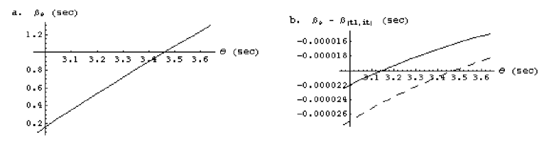
FIG. 3.: a. Exact angular position of the source, $\beta$, as a function of the image position, $\theta$, in arc sec. b. Error in the angular position of the source as a function of $\theta$. The first iterate error ($\beta_{ex}-\beta_{it}$) and the thin lens approximation error ($\beta_{ex}-\beta_{tl}$) are represented by a smooth line and a dashed line respectively, in arc sec.

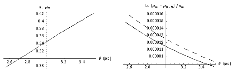
FIG. 4.: a. Exact magnification as a function of $\theta$. b. Relative errors in the magnifications predicted by the first iterate and thin lens are represented by smooth and dashed lines, respectively, as a function of $\theta$.

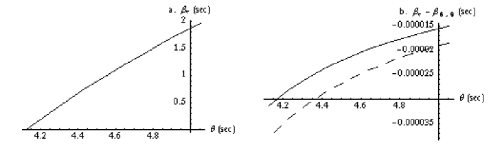
FIG. 5.: a. Exact angular position of the source, $\beta$, as a function of the image position for two lenses separated by a distance equal to the separation of the first lens and observer when the light ray does not cross the optical axis. b. Errors in the angular position of the source predicted by the first iterate and thin lens, represented by smooth and dashed lines, respectively.

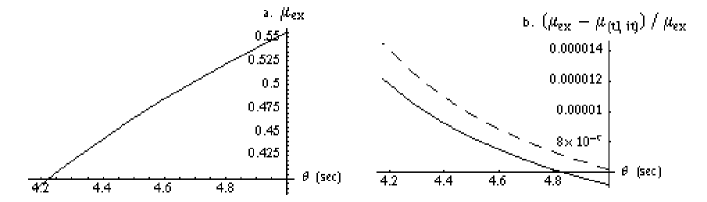
FIG. 6.: a. Exact magnification as a function of $\theta$ for two lenses separated by a distance equal to the separation of the first lens and observer when the light ray does not cross the optical axis. b. Relative errors in the magnifications predicted by the first iterate and thin lens, represented by smooth and dashed lines, respectively.

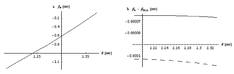
FIG. 7.: a. Exact angular position of the source, $\beta$, as a function of the image position for two lenses separated by a distance equal to the separation of the first lens and observer when the light ray crosses the optical axis. b. Errors in the angular position of the source predicted by the first iterate and thin lens, represented by smooth and dashed lines, respectively.

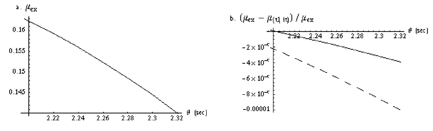
FIG. 8.: a. Exact magnification as a function of $\theta$ for two lenses separated by a distance equal to the separation of the first lens and observer when the light ray crosses the optical axis. b. Relative errors in the magnifications predicted by the first iterate and thin lens, represented by smooth and dashed lines, respectively.

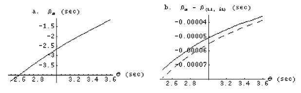
FIG. 9.: a. Exact angular position of the source, $\beta$, as a function of the image position for two lenses separated by a small distance compared with the separation of the first lens and observer. b. Errors in the angular position of the source predicted by the first iterate and thin lens, represented by smooth and dashed lines, respectively.

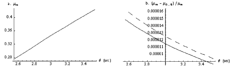
FIG. 10.: a. Exact magnification as a function of $\theta$ for two lenses separated by a small distance compared with the separation of the first lens and observer. b. Relative errors in the magnifications predicted by the first iterate and thin lens, represented by smooth and dashed lines, respectively.

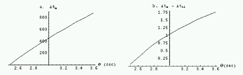
FIG. 11.: a. Exact time delay as a function of $\theta_{1}$ for two lenses separated by a small distance compared with the separation of the first lens and observer when $\theta_{2}=2.475^{\prime\prime}$. b. Error in the time delay predicted by the thin lens approximation when the two lenses are compressed into one lens plane.

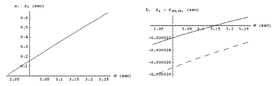
FIG. 12.: a. Exact angular position of the source $\beta$ as a function of the image position for two lenses in the same lens plane. b. Errors in the angular position of the source predicted by the first iterate and thin lens, represented by smooth and dashed lines, respectively.

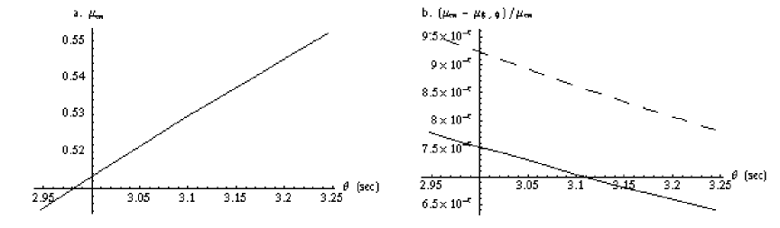
FIG. 13.: a. Exact magnification as a function of $\theta$ for two lenses in the same lens plane. b. Relative errors in the magnifications predicted by the first iterate and thin lens, represented by smooth and dashed lines, respectively.

REFERENCES

- [1] S. Frittelli and E. T. Newman, Phys. Rev. D 59, 124001, (1999).
- [2] T. P. Kling, E. T. Newman and A. Perez, Phys. Rev. D 61, (2000).
- [3] S. Frittelli, T. .P. Kling, and E. T. Newman, Phys. Rev. D 61, 064021, (2000).
- [4] K. S. Virbhadra and G. F. R. Ellis, astro-ph/9904193.
- [5] T. Pyne and M. Birkinshaw, ApJ, 415, 459, (1993).
- [6] T. Pyne and M. Birkinshaw, ApJ, 458, 46, (1996).
- [7] P. Schneider, J. Ehlers, and E. E. Falco, Gravitational Lenses, (Springer-Verlag, New York, Berlin, Heidelberg, 1992).
- [8] R. Blandford and R. Narayan, ApJ 310, 568-582, (1986).
- [9] Harvard-Smithsonian Center for Astrophysics website for lensing, http://cfa-www.harvard.edu/castles/.
- [10] T. P. Kling and E. T. Newman, Phys. Rev D 59, 124002, (1999).