Cosmological Time in (2+1)-Gravity

Abstract

We consider maximal globally hyperbolic flat (2+1) spacetimes with compact space $\displaystyle S$ of genus $\displaystyle g>1$. For any spacetime $\displaystyle M$ of this type, the length of time that the events have been in existence is $\displaystyle M$ defines a global time, called the cosmological time CT of $\displaystyle M$, which reveals deep intrinsic properties of spacetime. In particular, the past/future asymptotic states of the cosmological time recover and decouple the linear and the translational parts of the $\displaystyle ISO(2,1)$-valued holonomy of the flat spacetime. The initial singularity can be interpreted as an isometric action of the fundamental group of $\displaystyle S$ on a suitable real tree. The initial singularity faithfully manifests itself as a lack of smoothness of the embedding of the CT level surfaces into the spacetime $\displaystyle M$. The cosmological time determines a real analytic curve in the Teichmüller space of Riemann surfaces of genus $\displaystyle g$, which connects an interior point (associated to the linear part of the holonomy) with a point on Thurston’s natural boundary (associated to the initial singularity).

Dipartimento di Matematica, Università di Pisa, Via F. Buonarroti, 2, I-56127 PISA

Email: benedett@dm.unipi.it

Dipartimento di Fisica, Università di Pisa, Via F. Buonarroti, 2, I-56127 PISA

Email: guada@df.unipi.it

PACS: 04.60.Kz

Keywords: cosmological time, asymptotic states, real trees, marked spectra.

1 Introduction.

We shall be mainly concerned with maximal globally hyperbolic, matter-free spacetimes $\displaystyle M$ of topological type $\displaystyle S\times\mathbb{R}$, where $\displaystyle S$ is a compact closed oriented surface of genus $\displaystyle g>1$. The (2+1)-dimensional Einstein equation with vanishing cosmological constant actually implies that $\displaystyle M$ is (Riemann) flat.

After [D-J-’t H] and [W], a large amount of literature has grown up about this $\displaystyle(2+1)$-gravity topic, regarded as a useful toy-model for the higher dimensional case. Two main kinds of description have been experimented. A “cosmological” approach points to characterize the spacetimes in terms of some distinguished global time; for instance the constant mean curvature CMC time has been widely studied [A-M-T], [Mo]. A “geometric” time-free approach eventually identifies each flat spacetime by means of its $\displaystyle ISO(2,1)$-valued holonomy [W], [Me]. With the exception of the case with toric space ($\displaystyle g=1$), there is not a clear correspondence between the results obtained in these two approaches.

The aim of this paper is to show that this gap can be filled by using the canonical Cosmological Time CT, that is “the length of time that the events of $\displaystyle M$ have been in existence” (see [A-G-H]). It turns out that this is a global time which reveals the fundamental properties of spacetime. It is canonically defined by means of the very basic spacetime’s structures: its casual structure and the Lorentz distance. The cosmological time $\displaystyle\tau$ is invariant under diffeomorphisms, therefore the $\displaystyle\tau=a$ level surfaces $\displaystyle S_{a}$ provide a gauge-invariant description of space evolution in $\displaystyle M$. Both the intrinsic and extrinsic geometry of the surfaces $\displaystyle S_{a}$, as well as their past/future asymptotic states, are intrinsic features of spacetime. The asymptotic states are defined by the evolution of the observables associated to the length of closed geodesic curves on the surfaces $\displaystyle S_{a}$. Remarkably, they recover and decouple the linear and the translational parts of the holonomy. The study of the asymptotic states also leads to understand the initial singularity (we will always assume that the space is future expanding) and the way how the classical geometry degenerates, but does not completely disappear. The initial singularity can be interpreted as the isometric action of the fundamental group of $\displaystyle S$ on a suitable “real tree”. Differently to the case of the CMC time (for instance), the level surfaces $\displaystyle S_{a}$ of the CT are in general only $\displaystyle C^{1}$-embedded into the spacetime $\displaystyle M$. This lack of smoothness takes place on a “geodesic lamination” on $\displaystyle S_{a}$ and is a observable large scale manifestation of the intrinsic geometry of the initial singularity. Thus the initial singularity admits two complementary descriptions: one, in terms of real trees and, the second, in terms of geodesic laminations. The existence of a duality relation between real trees and laminations was already known in the context of Thurston theory of the boundary of the Teichmüller space. It is remarkable that Einstein theory of (2+1)-gravity sheds new light on this subject and puts duality in concrete form.

In [B-G2] we have also used the cosmological time in order to study certain interesting families of $\displaystyle(2+1)$-spacetimes coupled to particles.

Our main purpose consists of elucidating the central role of the cosmological time and its asymptotic states in the description of spacetimes. The cosmological time perspective provides a new interpretation of several facts spread in the literature which are related to Thurston work. More precisely, the present article is based on, and could be considered a complement of, Mess’s fundamental paper [Me].

2 The Cosmological Time Function.

For the basic notions of Lorentzian geometry and causality we refer for instance to [B-E], [H-E]. Let $\displaystyle N$ be any time oriented Lorentzian manifold of dimension $\displaystyle n+1$. The cosmological time function, $\displaystyle\tau:N\to(0,\infty]$, is defined as follows. Let $\displaystyle C^{-}(q)$ be the set of past-directed causal curves in $\displaystyle N$ that start at $\displaystyle q\in N$, then

$$\tau(q)={\rm sup}\,\{L(c):\ c\in C^{-}(q)\}$$

where $\displaystyle L(c)$ denotes the Lorentzian length of the curve $\displaystyle c\,$:

$$L(c)=\int_{c}\ (\,{\rm proper-time}\,)\ \ .$$

$\displaystyle\tau(q)$ can be interpreted as the length of time the event $\displaystyle q$ has been in existence in $\displaystyle N$. For example, if $\displaystyle N$ is the standard flat Minkowski space $\displaystyle\mathbb{M}^{n+1}$, $\displaystyle\tau$ is the constant $\displaystyle\infty$-valued function, so in this case it is not very interesting. In [A-G-H] (see also [W-Y]) one studies the properties of a manifold $\displaystyle N$ with regular cosmological time function. Recall that $\displaystyle\tau$ is regular if:

1) $\displaystyle\tau(q)$ is finite valued for every $\displaystyle q\in N$;

2) $\displaystyle\tau\to 0$ along every past directed inextensible causal curve.

The existence of a regular cosmological time function has strong consequences on the structure of $\displaystyle N$ and of the constant-$\displaystyle\tau$ surfaces [A-G-H]. In particular when $\displaystyle\tau$ is regular, $\displaystyle\tau:N\to(0,\infty[$ is a continuous function, which is twice differentiable almost everywhere, giving a global time on $\displaystyle N$ denoted by CT. Each $\displaystyle\tau$ level surface is a future Cauchy surface, so that $\displaystyle N$ is globally hyperbolic. For each $\displaystyle q\in N$ there exists a future-directed time-like unit speed geodesic ray $\displaystyle\gamma_{q}:(0,\tau(q)]\to N$ such that:

$$\gamma_{q}(\tau(q))=q\qquad,\qquad\tau(\gamma_{q}(t))=t\quad.$$

The union of the past asymptotic end-points of these rays can be regarded as the initial singularity of $\displaystyle N$.

The cosmological time function is not related to any specific choice of coordinates in $\displaystyle N$; it is “gauge-invariant” and so it represents an intrinsic feature of spacetime. Thus, when the cosmological time is regular, the $\displaystyle\tau$-constant level surfaces and their properties have a direct physical meaning as they are observables.

We present now two basic examples of spacetime with regular cosmological time, which shall be important throughout all the paper. To fix the notations, the standard Minkowski space $\displaystyle\mathbb{M}^{2+1}$ is endowed with coordinates $\displaystyle\,x=(x^{1},x^{2},x^{3})$, so that the metric is given by $\displaystyle ds^{2}=(dx^{1})^{2}+(dx^{2})^{2}-(dx^{3})^{2}$. $\displaystyle\mathbb{M}^{2+1}$ is oriented and time-oriented in the usual way.

Example 1. Consider the chronological future of the origin $\displaystyle 0\in\mathbb{M}^{2+1}$

$$I^{+}(0)=\{x\in\mathbb{M}^{2+1}:(x^{1})^{2}+(x^{2})^{2}-(x^{3})^{2}<0,\ x^{3}>0\}.$$

Its cosmological time, $\displaystyle\tau:I^{+}(0)\to(0,\infty)$, is a smooth submersion; the constant-time $\displaystyle\{\tau=a\}$ surfaces are the (upper) hyperboloids

$$\mathbb{I}(a)=\{x\in\mathbb{M}^{2+1}:(x^{1})^{2}+(x^{2})^{2}-(x^{3})^{2}=-a^{2},\ x^{3}>0\}.$$

Hence $\displaystyle\mathbb{I}(a)$ is a complete space of constant Gaussian curvature equal to $\displaystyle-1/a^{2}$, and of constant extrinsic mean curvature $\displaystyle 1/a$. The Lorentzian length of the time-like geodesic arc connecting any $\displaystyle p\in I^{+}(0)$ with $\displaystyle 0$ equals $\displaystyle\tau(p)$; $\displaystyle 0$ is the initial singularity. Note that $\displaystyle\mathbb{I}(a)$ can be obtained from $\displaystyle\mathbb{I}(1)$ by means of a dilatation in $\displaystyle\mathbb{M}^{2+1}$ with constant factor $\displaystyle a$; shortly we write $\displaystyle\mathbb{I}(a)=a\mathbb{I}(1)$. We shall denote by $\displaystyle SO(2,1)$ the group of oriented Lorentz transformations acting on $\displaystyle\mathbb{M}^{2+1}$ and by $\displaystyle ISO(2,1)$ the Poincaré group. $\displaystyle SO^{+}(2,1)$ denotes the subgroup of $\displaystyle SO(2,1)$ transformations which keep $\displaystyle I^{+}(0)$ and each $\displaystyle\mathbb{I}(a)$ invariant. $\displaystyle ISO^{+}(2,1)$ is the corresponding subgroup of $\displaystyle ISO(2,1)$.

Example 2. Let us denote by $\displaystyle I^{+}(1,3)$ the chronological future in $\displaystyle\mathbb{M}^{2+1}$ of the line $\displaystyle\{\ x^{1}=x^{3}=0\ \}$

$$I^{+}(1,3)=\{x\in\mathbb{M}^{2+1}:(x^{1})^{2}-(x^{3})^{2}<0,\ x^{3}>0\}\ .$$

The Lorentzian length of the time-like geodesic arc connecting any $\displaystyle p=(x^{1},x^{2},x^{3})\in I^{+}(1,3)$ with $\displaystyle q=(0,x^{2},0)$ equals the cosmological time $\displaystyle\tau(p)$. The level surfaces are

$$\mathbb{I}(1,3,a)=\{x\in\mathbb{M}^{2+1}:(x^{1})^{2}-(x^{3})^{2}=-a^{2},\ x^{3}>0\}$$

and have constant extrinsic mean curvature equal to $\displaystyle(1/2a)$. Each surface $\displaystyle\mathbb{I}(1,3,a)$ is isometric to the flat plane $\displaystyle\mathbb{R}^{2}$. To make this manifest, it is useful to consider the following change of coordinates. Let $\displaystyle\Pi^{2+1}=\{(u,y,\tau)\in\mathbb{R}^{2+1}:\tau>0\}$ be endowed with the metric $\displaystyle ds^{2}=\tau^{2}du^{2}+dy^{2}-d\tau^{2}$. Then, $\displaystyle x^{1}=\tau sh(u),\ x^{2}=y,\ x^{3}=\tau ch(u)$, is an isometry between $\displaystyle\Pi^{2+1}$ and $\displaystyle I^{+}(1,3)$. The level set $\displaystyle\{\tau=a\}$ of $\displaystyle\Pi^{2+1}$ goes isometrically onto $\displaystyle\mathbb{I}(1,3,a)$, so this is intrinsically flat. Note that the group of oriented isometries of $\displaystyle\Pi^{2+1}$ is generated by the translations parallel to the planes $\displaystyle\{\tau=a\}$, and the rotation of angle $\displaystyle\pi$ of the $\displaystyle(u,y)$ coordinates.

We are going to show that any maximal globally hyperbolic, matter-free $\displaystyle(2+1)$-spacetime $\displaystyle M$, with compact space $\displaystyle S$, actually has regular cosmological time, and its initial singularity can be accurately described.

3 Flat (2+1)-spacetimes

A flat spacetime is, by definition, locally isometric to the Minkowski space $\displaystyle\mathbb{M}^{2+1}$. We assume that our maximal hyperbolic flat spacetimes are time-oriented and future expanding, and that these orientations locally agree with the usual ones on $\displaystyle\mathbb{M}^{2+1}$. The spacetime structures on $\displaystyle S\times\mathbb{R}$ are regarded up to oriented isometry homotopic to the identity.

3.1 Minkowskian suspensions

We introduce here the simplest $\displaystyle(2+1)$ spacetimes with compact space $\displaystyle S$ of genus $\displaystyle g>1$.

Recall that the upper hyperboloid $\displaystyle\mathbb{I}(1)\subset\mathbb{M}^{2+1}$, mentioned in the previous section, is a classical model for the hyperbolic plane $\displaystyle\mathbb{H}^{2}$ (see [B-P] for this and other models); the Poincaré disk is another model which can be obtained from $\displaystyle\mathbb{I}(1)$ by means of the stereographic projection shown in figure 1. We shall use the Poincaré model in section 4.

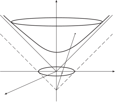
Figure 1: The hyperbolic plane in the hyperboloid and disk models.

Take any hyperbolic surface $\displaystyle F=\mathbb{H}^{2}/\Gamma$ homeomorphic to $\displaystyle S$. $\displaystyle\Gamma$ is a subgroup of $\displaystyle SO^{+}(2,1)$ which acts freely and properly discontinuously on $\displaystyle\mathbb{H}^{2}\cong\mathbb{I}(1)$. $\displaystyle\mathbb{I}(1)$ can be identified with the universal covering of $\displaystyle S$ and $\displaystyle\Gamma$ with the fundamental group $\displaystyle\pi_{1}(S)$. $\displaystyle\Gamma$ can be thought also as a group of isometries of the spacetime $\displaystyle I^{+}(0)$ and $\displaystyle M(F)=I^{+}(0)/\Gamma$ is the required spacetime with compact space homeomorphic to $\displaystyle S$. We call it the Minkowskian suspension of $\displaystyle F$. This construction is well-known; sometimes $\displaystyle M(F)$ is also called the Lorentzian cone over $\displaystyle F$ or the Löbell spacetime based on $\displaystyle F$. $\displaystyle I^{+}(0)$ can be regarded as the universal covering of $\displaystyle M(F)$. Let us now consider the cosmological time of $\displaystyle M(F)$. The CT of $\displaystyle I^{+}(0)$ naturally induces the CT of $\displaystyle M(F)$. Indeed, each level surface $\displaystyle S_{a}$ of $\displaystyle M(F)$ has $\displaystyle\mathbb{I}(a)$ as universal covering; moreover, $\displaystyle S_{1}=F$ and $\displaystyle S_{a}=aF$. In this case, the CT coincides with the CMC time and each level surface $\displaystyle S_{a}$ smoothly embeds into $\displaystyle M(F)$. The initial singularity “trivially” consists of one point.

Notation. Let $\displaystyle Y$ be any subset of $\displaystyle\mathbb{I}(1)$, we shall denote by $\displaystyle\widehat{Y}$ its “suspension” in $\displaystyle I^{+}(0)$ which is defined by $\displaystyle\widehat{Y}=\cup_{a\in(0,\infty[}\ aY$.

3.2 (2+1) spacetimes as deformed Minkowskian suspensions

It has been shown in [Me] that any maximal globally hyperbolic, future expanding flat spacetime $\displaystyle M$ with compact space homeomorphic to $\displaystyle S$, as above, can be regarded as a “deformation” of some Minkowskian suspension (see also [W]). In fact $\displaystyle M$ is of the form $\displaystyle M=U(M)/\Gamma^{\prime}$, where:

1) The domain $\displaystyle U(M)$ of $\displaystyle\mathbb{M}^{2+1}$ is a convex set

$$U(M)=\{x\in\mathbb{M}^{2+1};x^{3}>f(x)\}$$

where $\displaystyle f:\{x^{3}=0\}\to[0,\infty[$ is a convex function.

2) $\displaystyle\Gamma^{\prime}$ is a subgroup of $\displaystyle ISO^{+}(2,1)$ (also called the holonomy group of $\displaystyle M$) acting freely and properly discontinuously on $\displaystyle U(M)$. Hence $\displaystyle U(M)$ is the universal covering of $\displaystyle M$ and $\displaystyle\Gamma^{\prime}$ is isomorphic to $\displaystyle\pi_{1}(M)\cong\pi_{1}(S)$.

3) The “linear part” $\displaystyle\Gamma$ of $\displaystyle\Gamma^{\prime}$ is a subgroup of $\displaystyle SO^{+}(2,1)$ which is isomorphic to $\displaystyle\pi_{1}(S)$ and acts freely and properly discontinuously on $\displaystyle\mathbb{I}(1)\cong\mathbb{H}^{2}$. This is a non trivial fact which follows from a result of Goldman [Go]. Each element $\displaystyle\gamma^{\prime}\in\Gamma^{\prime}$ is of the form $\displaystyle\gamma^{\prime}=\gamma+t(\gamma)$, where $\displaystyle\gamma\in\Gamma$ and $\displaystyle t(\gamma)\in\mathbb{R}^{3}$ is a translation. $\displaystyle t:\Gamma\to\mathbb{R}^{3}$ is a cocycle representing an element of $\displaystyle H^{1}(\Gamma,\mathbb{R}^{3})$. If $\displaystyle t^{\prime}=\lambda t$, $\displaystyle\lambda\in\mathbb{R}^{*}$, then $\displaystyle U(M^{\prime})$ differs from $\displaystyle U(M)$ by : $\displaystyle U(M)=\lambda^{-1}U(M^{\prime})$. When $\displaystyle\lambda$ is “small”, $\displaystyle U(M^{\prime})$ is “close” to $\displaystyle I^{+}(0)$ ($\displaystyle M^{\prime}$ is “close” to $\displaystyle M(F)$, $\displaystyle F=\mathbb{H}^{2}/\Gamma$).

Note that $\displaystyle\Gamma^{\prime}$, whence $\displaystyle U(M)$ and $\displaystyle t$, are defined up to inner automorphism of $\displaystyle ISO^{+}(2,1)$.

3.3 Spacetimes of simplicial type

In this section, we shall consider the flat spacetimes that can be obtained from Minkowskian suspensions by means of particular deformations. These spacetimes will be called of simplicial type, the origin of this name is related to the material presented in section 4. Spacetimes of simplicial type are important because they are “dense” in the set of all spacetimes; the shape of any spacetime and of its CT can be arbitrarily well approximated by some spacetime of simplicial type (see proposition 4.23). So, it is enough to understand these examples in order to have a rather complete qualitative picture of our general presentation. Moreover, all the statements of this paper can easily be checked in a spacetime of simplicial type.

Start with a Minkowskian suspension $\displaystyle M(F)$. Assume that a weighted multi-curve $\displaystyle\mathcal{L}$ on $\displaystyle F$ is given. $\displaystyle\mathcal{L}$ is the union of a finite number of disjoint simple closed geodesics on $\displaystyle F$, each one endowed with a strictly positive real weight. $\displaystyle\mathcal{L}$ governs a specific deformation of $\displaystyle M(F)$ producing a required flat spacetime denoted by $\displaystyle M(F,\mathcal{L})$. A particular spacetime deformation is associated to each component of $\displaystyle\mathcal{L}$ and can be obtained by means of an appropriate surgery operation in Minkowski space. As the deformations associated to the components of $\displaystyle\mathcal{L}$ act locally and independently from each other, we may assume for simplicity that $\displaystyle\mathcal{L}$ just consists of one component $\displaystyle c$, with weight $\displaystyle r$ and length $\displaystyle s$.

Elementary deformation. In order to illustrate the deformation associated with one geodesic $\displaystyle c$ with weight $\displaystyle r$, we shall now introduce a simple hyperbolic surface $\displaystyle F_{0}$ which can be understood as a local model for the general surface $\displaystyle S$. Let $\displaystyle\Gamma_{0}$ be an infinite cyclic subgroup of $\displaystyle SO^{+}(2,1)$ generated by an element $\displaystyle g_{0}$ acting on $\displaystyle\mathbb{I}(1)$ as an isometry of hyperbolic type (see for instance [B-P] for the classification of the isometries of $\displaystyle\mathbb{H}^{2}$). We can assume that $\displaystyle g_{0}$ is a Lorentz transformation corresponding to a boost along the $\displaystyle x^{1}$-direction, so that the $\displaystyle g_{0}$-invariant geodesic line on $\displaystyle\mathbb{I}(1)$ is the line $\displaystyle\sigma_{0}=\mathbb{I}(1)\cap\{x^{2}=0\}$. The hyperbolic surface $\displaystyle F_{0}=\mathbb{I}(1)/\Gamma_{0}$ is homeomorphic to the non-compact annulus $\displaystyle S^{1}\times\mathbb{R}$ and its area is not finite. The image in $\displaystyle F_{0}$ of the axis of $\displaystyle g_{0}$ is a simple closed geodesic $\displaystyle c$ of a certain length $\displaystyle s$; give it the positive weight $\displaystyle r$. So we dispose of a one-component weighted multi-curve $\displaystyle\mathcal{L}_{0}$ on $\displaystyle F_{0}$, as illustrated in figure 2.

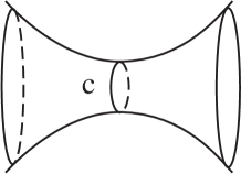
Figure 2: The surface $\displaystyle F_{0}$ with the closed geodesic $\displaystyle c$.

The suspension $\displaystyle M(F_{0})=I^{+}(0)/\Gamma_{0}$ is a flat spacetime. Let us now construct $\displaystyle M_{0}=M(F_{0},\mathcal{L}_{0})$ which represents the deformation of $\displaystyle M(F_{0})$ associated to the weighted multi-curve $\displaystyle\mathcal{L}_{0}$. We shall use the spacetimes $\displaystyle I^{+}(0)$, $\displaystyle I^{+}(1,3)$ and $\displaystyle\Pi^{2+1}$ that we have introduced in section 2. The universal covering $\displaystyle U(M_{0})$ of $\displaystyle M_{0}$ will be the union of three domains of $\displaystyle\mathbb{M}^{2+1}$: $\displaystyle U(M_{0})=A\cup B\cup C$, where $\displaystyle A=I^{+}(0)\cap\{x^{2}\leq 0\}$, $\displaystyle B=I^{+}(1,3)\cap\{0\leq x^{2}\leq r\}$, $\displaystyle C=C^{\prime}+r(0,1,0)$ and $\displaystyle C^{\prime}=I^{+}(0)\cap\{x^{2}\geq 0\}\$. In our notations, $\displaystyle C^{\prime}+r(0,1,0)$ denotes the set of points in $\displaystyle\mathbb{M}^{2+1}$ which can be obtained from $\displaystyle C^{\prime}$ by means of a translation of length $\displaystyle r$ along the unit vector $\displaystyle(0,1,0)$. It is important to note that the cosmological times of the different pieces $\displaystyle A$, $\displaystyle B$ and $\displaystyle C$ fit well together; in fact, the CT level surfaces $\displaystyle\widetilde{S}_{a}$ of $\displaystyle U(M_{0})$ are

$$\widetilde{S}_{a}=(a\mathbb{I}(1)\cap\{x^{2}<0\})\cup(\mathbb{I}(1,3,a)\cap\{0\leq x^{2}\leq r\})\cup(a\mathbb{I}(1)\cap\{x^{2}>0\}+r(0,1,0))\ .$$

As shown in figure 3, each surface $\displaystyle\widetilde{S}_{a}\subset\mathbb{M}^{2+1}$ can be obtained by cutting the hyperboloid $\displaystyle\mathbb{I}(a)$ along $\displaystyle a\sigma_{0}$ (which is the intersection of $\displaystyle\mathbb{I}(a)$ with the $\displaystyle\{x^{2}=0\}$-plane) and then by inserting a band of $\displaystyle\mathbb{I}(1,3,a)$ of depth $\displaystyle r\,$.

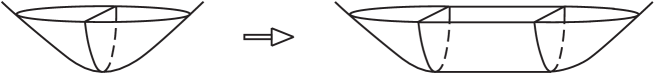
Figure 3: Level surfaces $\displaystyle\widetilde{S}_{a}$ of $\displaystyle U(M_{0})$.

The surfaces $\displaystyle\widetilde{S}_{a}$ are only $\displaystyle C^{1}$-embedded into $\displaystyle U(M_{0})$. The initial singularity of $\displaystyle U(M_{0})$ is the segment $\displaystyle J_{0}=\{\ x^{1}=x^{3}=0\,\ \ 0\leq x^{2}\leq r\}$.

Remark 3.1

We have the following characterization of $\displaystyle J_{0}$. The interior points of this segment make the subset of $\displaystyle\partial U(M_{0})$ (boundary of the convex set $\displaystyle U(M_{0})$) of the points with exactly two null supporting planes; the end-points make the subset of $\displaystyle\partial U(M)$ with more than two null supporting planes. Recall that a supporting plane at $\displaystyle x\in\partial U(M_{0})$ is a plane $\displaystyle P$ such that $\displaystyle x\in P$ and $\displaystyle U(M_{0})\cap P=\emptyset$. $\displaystyle P$ is null if it contains some null-lines.

The covering $\displaystyle U(M_{0})\subset\mathbb{M}^{2+1}$ is flat. To get $\displaystyle M_{0}$, we only need to specify the action of $\displaystyle\pi_{1}=\pi_{1}(F_{0})\cong\mathbb{Z}$ on $\displaystyle U(M_{0})$.

Action of the fundamental group. $\displaystyle\pi_{1}$ acts on $\displaystyle A$ by the restriction of the action of $\displaystyle\Gamma_{0}$ on $\displaystyle\mathbb{I}(1)$. The domain $\displaystyle B$ corresponds (via the isometry established in section 2) to $\displaystyle B^{\prime}=\{(u,y,\tau)\in\Pi^{2+1};0\leq y\leq r\}$, so that the action of $\displaystyle\pi_{1}$ on $\displaystyle B$ transported on $\displaystyle B^{\prime}$ is just given by the translation $\displaystyle(u,y,\tau)\to(u+s,y,\tau)$. Finally, if $\displaystyle\alpha$ is the translation $\displaystyle(x^{1},x^{2},x^{3})\to(x^{1},x^{2}+r,x^{3})$ on $\displaystyle\mathbb{M}^{2+1}$, then the action of $\displaystyle\pi_{1}$ on $\displaystyle C$ is just the conjugation of $\displaystyle\Gamma_{0}$ by $\displaystyle\alpha$.

The CT of the covering $\displaystyle U(M_{0})$ passes to the quotient $\displaystyle M_{0}=U(M_{0})/\pi_{1}$; each level surface $\displaystyle S_{a}$ is only $\displaystyle C^{1}$-embedded into $\displaystyle M_{0}$, so that it is endowed with an induced $\displaystyle C^{1}$-Riemannian metric. This allows anyway to define the length of curves traced on the surface $\displaystyle S_{a}$ and the derived length-space distance. Let $\displaystyle\mathcal{A}=A/\pi_{1}$, $\displaystyle\mathcal{B}=B/\pi_{1}$ and $\displaystyle\mathcal{C}=C/\pi_{1}$. Then, $\displaystyle S_{a}\cap\mathcal{B}$ is a flat annulus of depth $\displaystyle r$ and parallel geodesic boundary components of length $\displaystyle as\,$; $\displaystyle S_{a}\cap(\mathcal{A}\cup\mathcal{C})$ can be isometrically embedded into $\displaystyle aF_{0}$, and has geodesic boundary curves of length $\displaystyle as$. As shown in figure 4, $\displaystyle S_{a}$ can be obtained by cutting $\displaystyle F_{0}$ along $\displaystyle c$ and by inserting a annulus of depth $\displaystyle r$.

Figure 4: Level surface of $\displaystyle M_{0}$.

Remark 3.2

If $\displaystyle g$ is an element of $\displaystyle ISO^{+}(2,1)$ acting on $\displaystyle X\in\mathbb{M}^{2+1}$ as $\displaystyle g(X)=QX+w$, the transformed domain $\displaystyle g(U(M_{0}))=Q(A\cup B\cup C)+w$ is, of course, an isometric copy of the universal covering in $\displaystyle\mathbb{M}^{2+1}$. The curve $\displaystyle\sigma=Q(\sigma_{0})$ is a geodesic line of $\displaystyle\mathbb{I}(1)$; $\displaystyle\sigma$ is the intersection of $\displaystyle\mathbb{I}(1)$ with a suitable hyperplane passing at the origin of $\displaystyle\mathbb{M}^{2+1}$. Let us denote by $\displaystyle\widehat{\sigma}$ the suspension of $\displaystyle\sigma\,$; then

$$Q(B)=\cup_{\lambda\in[0,r]}\ \{\widehat{\sigma}+\lambda v\}$$

where $\displaystyle v$ is the unitary (in the Minkowski norm) vector tangent to $\displaystyle\mathbb{I}(1)$, normal to $\displaystyle\sigma$, and pointing towards $\displaystyle Q(C^{\prime})$. We also denote $\displaystyle Q(B)=B(\sigma,v,r)$. The shape of the CT level surfaces in $\displaystyle g(U(M_{0}))$ is shown in figure 5. The initial singularity of $\displaystyle g(U(M_{0}))$ is given by the space-like segment $\displaystyle J=Q(J_{0})+w$.

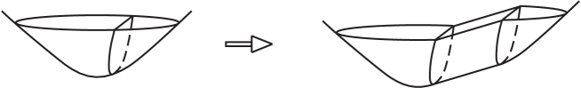
Figure 5: Level surfaces of $\displaystyle g(U(M_{0}))$.

Simplicial type deformation. $\displaystyle M_{0}$ represents a local model of the deformation $\displaystyle M=M(F,\mathcal{L})$ we are interested in. In fact, there exists a neighborhood $\displaystyle\mathcal{W}$ of $\displaystyle\mathcal{B}$ in $\displaystyle M_{0}$ which embeds isometrically into $\displaystyle M$, respecting the cosmological time. Let us denote by $\displaystyle\mathcal{W}^{\prime}$ the image of $\displaystyle\mathcal{W}$ in $\displaystyle M$. Then $\displaystyle M\setminus\mathcal{W}^{\prime}$ embeds isometrically into the Minkowskian suspension $\displaystyle M(F)$, respecting again the cosmological time.

We describe now the universal covering $\displaystyle U(M)\subset\mathbb{M}^{2+1}$ and a cocycle $\displaystyle t:\Gamma\to\mathbb{R}^{3}$ which leads to $\displaystyle\Gamma^{\prime}\subset ISO^{+}(2,1)$ such that $\displaystyle M=U(M)/\Gamma^{\prime}$. The inverse image of $\displaystyle c\subset F=\mathbb{I}(1)/\Gamma$ into the covering $\displaystyle\mathbb{I}(1)$ is an infinite and locally finite set $\displaystyle\widetilde{\mathcal{L}}$ of disjoint complete geodesic lines. Given any geodesic $\displaystyle\sigma_{0}\in\widetilde{\mathcal{L}}$, then $\displaystyle\widetilde{\mathcal{L}}=\{\sigma=\gamma(\sigma_{0});\gamma\in\Gamma\}$. Let $\displaystyle\widehat{\mathcal{L}}\subset I^{+}(0)$ be the suspension of the geodesic lines of $\displaystyle\widetilde{\mathcal{L}}$. The set $\displaystyle\mathbb{I}(1)\setminus\widetilde{\mathcal{L}}$ is the union of an infinite number of connected components. Denote by $\displaystyle R$ any such a component, and by $\displaystyle\widehat{R}$ its suspension, which is a component of $\displaystyle I^{+}(0)\setminus\widehat{\mathcal{L}}$. Every $\displaystyle R$ covers a component $\displaystyle F_{R}$ of $\displaystyle F\setminus\mathcal{L}$; more precisely, if $\displaystyle\Gamma_{R}$ is the subgroup of $\displaystyle\Gamma$ which keeps $\displaystyle R$ invariant, then $\displaystyle F_{R}=R/\Gamma_{R}$.

Now, fix one base component $\displaystyle R_{0}$ and take in it one base point $\displaystyle x_{0}$. For each $\displaystyle\gamma\in\Gamma$, let $\displaystyle\gamma(x_{0})$ be the point in $\displaystyle\mathbb{I}(1)$ which is defined by the action of $\displaystyle\gamma$ on $\displaystyle x_{0}$. The geodesic arc in $\displaystyle\mathbb{I}(1)$ connecting $\displaystyle x_{0}$ with $\displaystyle\gamma(x_{0})$ crosses a finite number of lines $\displaystyle\{\sigma_{i}\}$ belonging to $\displaystyle\widetilde{\mathcal{L}}$. At each crossing consider the unitary (in the norm of $\displaystyle\mathbb{M}^{2+1}$) vector $\displaystyle v_{i}$ tangent to $\displaystyle\mathbb{I}(1)$ and normal to $\displaystyle\sigma_{i}$, pointing far from $\displaystyle x_{0}$. Then, the required cocycle $\displaystyle t(\gamma)\in\mathbb{R}^{3}$ is given by

$$t(\gamma)=\sum_{i}rv_{i}\ .$$

Note that if $\displaystyle\gamma_{1}(x_{0})$ and $\displaystyle\gamma_{2}(x_{0})$ belong to the same component $\displaystyle R$, then $\displaystyle t(\gamma_{1})=t(\gamma_{2})$, whence also $\displaystyle t(R)=t(\gamma)$ for any $\displaystyle\gamma$ such that $\displaystyle\gamma(x_{0})\in R$, is well defined. $\displaystyle U(M)$ is tiled by tiles of two types: (i) “$\displaystyle\widehat{R}+w$”, (ii) “$\displaystyle B(\sigma,v,r)+w$”, for some translation vector $\displaystyle w\in\mathbb{R}^{3}$. More precisely, the tiles of the first type make the open subset of $\displaystyle U(M)$

$$\mathcal{R}=\cup_{R}\ \{\widehat{R}+t(R)\}\ .$$

Each line $\displaystyle\sigma\in\widetilde{\mathcal{L}}$ is in the boundary of two regions $\displaystyle R_{\sigma}$, $\displaystyle R^{\prime}_{\sigma}$ and we assume that $\displaystyle R_{\sigma}$ is closer to $\displaystyle x_{0}$ than $\displaystyle R^{\prime}_{\sigma}$. Set $\displaystyle v_{\sigma}$ the unitary (in the norm of $\displaystyle\mathbb{M}^{2+1}$) vector tangent to $\displaystyle\mathbb{I}(1)$ and normal to $\displaystyle\sigma$, pointing towards $\displaystyle R^{\prime}_{\sigma}$. The two regions $\displaystyle\widehat{R}_{\sigma}+t(R_{\sigma})$ and $\displaystyle\widehat{R}^{\prime}_{\sigma}+t(R^{\prime}_{\sigma})$ are connected by the tile of the second type $\displaystyle B(\sigma,v_{\sigma},r)+t(R_{\sigma})$, so that

$$U(M)\setminus\mathcal{R}=\cup_{\sigma\in\widetilde{\mathcal{L}}}\ (B(\sigma,v_{\sigma},r)+t(R_{\sigma}))\ .$$

Note that each tile has its own CT; all the cosmological times fit well together and define the CT of $\displaystyle U(M)$ which passes to the quotient $\displaystyle M$.

Remark 3.3

The construction of $\displaystyle M(F)$ and of $\displaystyle M(F,\mathcal{L})$ can be performed for any hyperbolic surface $\displaystyle F$, not necessarily compact nor of finite area. Similarly, by starting from any locally finite family of weighted geodesic lines in $\displaystyle\mathbb{I}(1)$, the simplicial deformation that we have just described produces a globally hyperbolic spacetime structure on $\displaystyle\mathbb{R}^{2}\times\mathbb{R}$ with a regular cosmological time.

Remark 3.4

When $\displaystyle F$ is compact, every region $\displaystyle R$ (defined above) is bounded by infinitely many lines of $\displaystyle\widetilde{\mathcal{L}}$. In fact, as $\displaystyle F$ is compact, every $\displaystyle\gamma\in\Gamma$ with $\displaystyle\gamma\neq 1$ is of hyperbolic type [B-P]. Consequently, for any $\displaystyle\sigma\in\widetilde{\mathcal{L}}$ and for every $\displaystyle\gamma\in\Gamma$ with $\displaystyle\gamma(\sigma)\neq\sigma$, $\displaystyle\sigma$ and $\displaystyle\gamma(\sigma)$ are “ultra-parallel”. This means that the hyperbolic distance satisfies $\displaystyle d(\sigma,\gamma(\sigma))>0$; moreover, $\displaystyle\sigma$ and $\displaystyle\gamma(\sigma)$ have a common orthogonal geodesic line. Suppose now that a region $\displaystyle R$ is bounded by finitely many lines in $\displaystyle\widetilde{\mathcal{L}}$. In this case, $\displaystyle R$ contains a band $\displaystyle E$ of infinite diameter, bounded by two half-lines contained in $\displaystyle\widetilde{\mathcal{L}}$. As $\displaystyle F$ is compact, $\displaystyle\mathbb{H}^{2}$ is tiled by tiles of the form $\displaystyle\gamma(\mathcal{D})$, where $\displaystyle\mathcal{D}$ is a fundamental domain for $\displaystyle\Gamma$ of finite diameter. So, one (at least) tile $\displaystyle\gamma(\mathcal{D})$ must be contained in $\displaystyle E$. But clearly $\displaystyle\gamma(\mathcal{D})\cap\widetilde{\mathcal{L}}\neq\emptyset$ and this contradicts the fact that $\displaystyle R$ is a region of $\displaystyle\mathbb{H}^{2}\setminus\widetilde{\mathcal{L}}$.

The same conclusion holds if $\displaystyle F$ is of finite area. If $\displaystyle F$ is of infinite area, we can eventually have different behaviours. For instance, in the example $\displaystyle F_{0}$ above, $\displaystyle\widetilde{\mathcal{L}}_{0}$ just consists of one component which divides $\displaystyle\mathbb{H}^{2}$ into two regions. Other examples will be presented in subsection 4.1.

4 The cosmological time of (2+1)-spacetimes

In this section we describe the main properties of the CT for an arbitrary spacetime $\displaystyle M$. We adopt the notations of the previous sections; in particular, $\displaystyle M$ is assumed to be an expanding matter-free spacetime of topological type $\displaystyle S\times\mathbb{R}$ with compact surface $\displaystyle S$ of genus $\displaystyle g>1$. The validity of the following statements can be quite easily checked for spacetimes of simplicial type. We shall try to point out the main ideas; we postpone a commentary on the proofs, with references to the existing literature.

Proposition 4.1

The cosmological time function, $\displaystyle\tau:M\to(0,\infty[$, is surjective and regular, so that it defines a global time on $\displaystyle M$. It lifts to a regular cosmological time on the covering, $\displaystyle\widetilde{\tau}:U(M)\to(0,\infty[$. Each level surface $\displaystyle\widetilde{S}_{a}$ of $\displaystyle U(M)$ maps onto $\displaystyle S_{a}$ of $\displaystyle M$ and is its universal covering. In other words, the action of $\displaystyle\pi_{1}(S)$ on $\displaystyle U(M)$ restricts to a free, properly discontinuous isometric action on $\displaystyle\widetilde{S}_{a}$ such that $\displaystyle S_{a}=\widetilde{S}_{a}/\pi_{1}(S)$. Each $\displaystyle\widetilde{S}_{a}$ ($\displaystyle S_{a}$) is a future Cauchy surface.

4.1 Initial singularity - external view

Let us give a description of the initial singularity of $\displaystyle M$ as it appears “from the exterior” point of view, that is, from the Minkowski space in which the universal covering $\displaystyle U(M)$ is placed. In subsection 4.5 we shall show how the initial singularity can also be characterized in terms of the observables associated with the CT asymptotic states.

Let us first give a definition.

Definition 4.2

An $\displaystyle\mathbb{R}$-tree (also called a real tree) is a metric space $\displaystyle(\mathcal{T},d)$ such that for each couple of points $\displaystyle p\neq q\in\mathcal{T}$ there exists a unique arc in $\displaystyle\mathcal{T}$ with $\displaystyle p$ and $\displaystyle q$ as end-points and this arc is isometric to the interval $\displaystyle[0,d(p,q)]\subset\mathbb{R}$. This arc is called a segment of $\displaystyle\mathcal{T}$ and is denoted $\displaystyle[p,q]$.

Remark 4.3

The so-called simplicial trees are the simplest examples of real trees. A simplicial tree is a real tree covered by a countable family of elementary segments, called the “edges” of the tree, in such a way that: a) whenever two edges intersect, then they just have one common endpoint; b) the edge-lengths take values in a finite set of strictly positive numbers. Any endpoint of any edge is called a “vertex” of the tree. The distance is the natural length-space distance. Note that a simplicial tree is not necessarily locally finite; in other words, vertices of infinite “valence” may occur. In general, a real tree is more complicated than a simplicial tree because one might find, for instance, a segment containing a Cantor set made by the endpoints of other segments.

Proposition 4.4

For any $\displaystyle p\in U(M)\subset\mathbb{M}^{2+1}$ there is a unique time-like geodesic arc $\displaystyle a(p)$ contained in $\displaystyle U(M)$, which starts at $\displaystyle p$ and is directed in the past of $\displaystyle p$, such that the Lorentzian length of $\displaystyle a(p)$ equals $\displaystyle\widetilde{\tau}(p)$. The other end-point of $\displaystyle a(p)$, denoted by $\displaystyle i(p)$, belongs to the boundary $\displaystyle\partial U(M)$ of $\displaystyle U(M)$ in $\displaystyle\mathbb{M}^{2+1}$. If $\displaystyle p$ and $\displaystyle q$ are identified in $\displaystyle M$ by the action of $\displaystyle\pi_{1}(S)$, so are $\displaystyle a(p)$ and $\displaystyle a(q)$. The union of the initial points $\displaystyle\mathcal{T}=\{i(p);p\in U(M)\ \}$ is an $\displaystyle\mathbb{R}$-tree. More precisely, each segment of $\displaystyle\mathcal{T}$ is a rectifiable space-like curve in $\displaystyle\partial U(M)$ with its own length. There is a natural isometric action of the fundamental group $\displaystyle\pi_{1}(S)$ on $\displaystyle\mathcal{T}$. The quotient space $\displaystyle i(M)=\mathcal{T}/\pi_{1}(S)$ can be thought as the initial singularity of $\displaystyle M$.

Remark 4.5

We have already encountered several examples of spaces of the form $\displaystyle X=\widetilde{X}/\pi_{1}(S)$ for some action of $\displaystyle\pi_{1}$ on $\displaystyle\widetilde{X}$: for instance, $\displaystyle F=\mathbb{H}^{2}/\Gamma$, $\displaystyle M=U(M)/\Gamma^{\prime}$, $\displaystyle S_{a}=\widetilde{S}_{a}/\Gamma^{\prime}$. Now, the initial singularity of spacetime also is a quotient $\displaystyle i(M)=\mathcal{T}/\pi_{1}(S)$. Instead of the bare topological quotient space, it is more interesting to consider $\displaystyle\widetilde{X}$ endowed with the action of $\displaystyle\pi_{1}$.

Remark 4.6

When $\displaystyle M$ is of simplicial type, the corresponding real tree $\displaystyle\mathcal{T}$ is actually a simplicial real tree. This justifies the name we have given to these special spacetimes. In this case, the set of edges of $\displaystyle\mathcal{T}$ consists of the union of the space-like segments which form the initial singularity of the different tiles of the form $\displaystyle B(\sigma,v_{\sigma},r)+t(R_{\sigma})$ (see section 3). The points of $\displaystyle\mathcal{T}$ can also be characterized by the properties discussed in remark 3.1. A homeomorphic (not isometric) copy of $\displaystyle\mathcal{T}$ can easily be embedded into $\displaystyle\mathbb{I}(1)$. Select one point in each region of $\displaystyle\mathbb{I}(1)\setminus\widetilde{\mathcal{L}}$ and consider the set made by the union of all these points. Connect two points of this set by a geodesic segment of $\displaystyle\mathbb{I}(1)$ if and only if they belong to adjacent regions. In this way we get the required tree. This tree is manifestly “dual” of $\displaystyle\widetilde{\mathcal{L}}$; in fact, the regions of $\displaystyle\mathbb{I}(1)\setminus\widetilde{\mathcal{L}}$ correspond to the vertices of $\displaystyle\mathcal{T}$ and the lines of $\displaystyle\widetilde{\mathcal{L}}$ correspond to the edges of $\displaystyle\mathcal{T}$. We shall return on this duality in section 4.3. Note that, as demonstrated in remark 3.4, all the vertices of $\displaystyle\mathcal{T}$ are of infinite valence.

Examples of real trees. A hyperbolic surface $\displaystyle F=\mathbb{H}^{2}/\Gamma$ is represented in figure 6. $\displaystyle F$ is of infinite area and is homeomorphic to a torus with one puncture; two simple closed geodesics $\displaystyle c$ and $\displaystyle a$ on $\displaystyle F$ are depicted. The geodesic $\displaystyle c$ cuts open $\displaystyle F$ into a compact surface and an infinite area annulus. By using the Poincaré disk model, a fundamental domain of $\displaystyle\Gamma$ in $\displaystyle\mathbb{H}^{2}$ is also shown in figure 6. This domain is delimited by four pair-wise ultra-parallel geodesic lines. The inverse images of $\displaystyle c$ and $\displaystyle a$ are represented on this domain. The first two terms of a sequence of partial tilings of $\displaystyle\mathbb{H}^{2}$, made by a finite number of copies of the fundamental domain, are shown in figure 7. The first partial tiling just contains one fundamental domain. The second is made by the union of $\displaystyle 1+4=5$ copies of the fundamental domain. The next partial tiling of this sequence, which is not shown in the figure, contains $\displaystyle 1+4+12=17$ tiles, and so on. For each partial tiling of $\displaystyle\mathbb{H}^{2}$ one can determine a corresponding partial lifting of the curves $\displaystyle c$ and $\displaystyle a$. Figure 8 shows the first two partial liftings $\displaystyle\widetilde{c}$ of $\displaystyle c$ and the structure of the associated partial dual trees. In the limit of the complete infinite tiling of $\displaystyle\mathbb{H}^{2}$, the complete lifting of $\displaystyle c$ contains an infinite number of geodesics and the associated real tree is infinite. In this case, $\displaystyle\mathbb{H}^{2}\setminus\widetilde{c}$ has exactly one component with infinitely many boundary lines (the associated vertex of the dual tree has infinite valence), whereas all the remaining components have one boundary line. The first three partial liftings $\displaystyle\widetilde{a}$ of $\displaystyle a$ are shown in figure 9; the corresponding partial dual trees are also represented. Note that these figures are just evocative, as they are not geometrically exact.

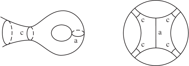
Figure 6: Two simple curves on $\displaystyle F=\mathbb{H}^{2}/\Gamma$.

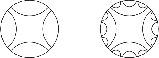
Figure 7: Partial tilings of $\displaystyle\widetilde{F}=\mathbb{H}^{2}$.

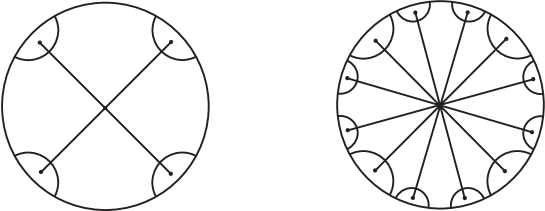
Figure 8: Partial $\displaystyle\widetilde{c}$ and dual trees.

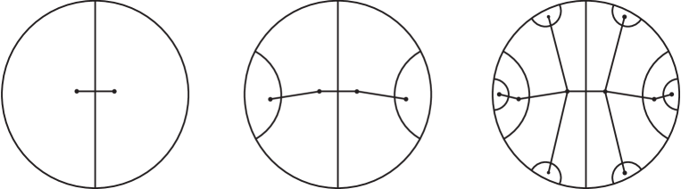
Figure 9: Partial $\displaystyle\widetilde{a}$ and dual trees.

Remark 4.7

The $\displaystyle\mathbb{R}$-trees and the associated $\displaystyle\pi_{1}(S)$-actions which occur in proposition 4.4 are not arbitrary (see [O] pag. 32). In fact, one can prove that the $\displaystyle\pi_{1}(S)$-action is minimal with small edge-stabilizers. This means that there is no non-empty strictly sub-tree which is invariant for this action, and that, for each segment in the tree, the subgroup of $\displaystyle\pi_{1}(S)$ which keeps the segment invariant is virtually Abelian. We shortly say that a real tree which admits such a kind of $\displaystyle\pi_{1}(S)$-action, is geometric.

4.2 Intrinsic and extrinsic geometry of the constant CT surfaces

In order to describe the geometric properties of the surfaces of constant cosmological time, it is natural to introduce the notion of geodesic lamination.

Definition 4.8

Let $\displaystyle G$ be a surface endowed with a $\displaystyle C^{1}$-Riemannian metric. As usual, this induces a length-space distance on $\displaystyle G$ and the notion of geodesic arc (line) makes sense. A geodesic lamination of $\displaystyle G$ is a closed subset $\displaystyle K$ of $\displaystyle G$, also called the support of the lamination, which is the disjoint union of complete and simple geodesics, also called the leaves of the lamination. “Complete” means that we dispose of arc-length parametrization defined on the whole real line $\displaystyle\mathbb{R}$; “simple” means that the geodesic has no self-normal crossing in $\displaystyle G$. In other words, each leaf is either a simple closed geodesic or a simple geodesic which is an isometric copy of $\displaystyle\mathbb{R}$ embedded in $\displaystyle G$. When $\displaystyle G$ is compact, such a non compact leaf is not a closed subset of $\displaystyle G$.

Remark 4.9

A finite union of disjoint simple closed geodesics is called a multi-curve and is the simplest example of geodesic lamination. We have already introduced multi-curves in section 3.3. A generic geodesic lamination $\displaystyle K$ can be more complicated than a multi-curve; in fact, if $\displaystyle\alpha$ is an arc embedded in $\displaystyle G$ which is transverse to the leaves of $\displaystyle K$, typically $\displaystyle\alpha\setminus K$ is a Cantor set.

Proposition 4.10

For every $\displaystyle a\in(0,\infty[$:

1) $\displaystyle\widetilde{S}_{a}$ is the graph of a positive convex function defined on the plane $\displaystyle\{x^{3}=0\}$ in $\displaystyle\mathbb{M}^{2+1}$.

2) $\displaystyle\widetilde{S}_{a}$ is only $\displaystyle C^{1}$-embedded into $\displaystyle U(M)$, so that it carries an induced $\displaystyle C^{1}$-Riemannian metric. $\displaystyle\widetilde{S}_{a}$ is geodesically complete and for each $\displaystyle p\neq q\in\widetilde{S}_{a}$, there is a unique geodesic arc connecting $\displaystyle p$ and $\displaystyle q$.

3) The locus $\displaystyle\widetilde{L}_{a}$ at which the embedding of $\displaystyle\widetilde{S}_{a}$ into $\displaystyle U(M)$ is no longer $\displaystyle C^{2}$ is a geodesic lamination of $\displaystyle\widetilde{S}_{a}$. $\displaystyle\widetilde{L}_{a}$ is in fact the pull-back of a geodesic lamination $\displaystyle L_{a}$ of $\displaystyle S_{a}$.

Remark 4.11

If $\displaystyle M$ is the spacetime of simplicial type which corresponds to the weighted multi-curve $\displaystyle\mathcal{L}$ on the surface $\displaystyle F$, then $\displaystyle L_{a}$ is just made by the boundary components of the flat annular components embedded into $\displaystyle S_{a}$, which are associated to the components of $\displaystyle\mathcal{L}$.

The content of the last remark generalizes as follows. Recall that $\displaystyle\pi_{1}(S)$ acts as $\displaystyle\Gamma$ on each $\displaystyle\mathbb{I}(a)$. For every $\displaystyle a\in(0,\infty[\,$, let us consider the map

$$p_{a}:\widetilde{S}_{a}\to\mathbb{I}(a)$$

defined as follows: $\displaystyle p_{a}(x)$ is the unique point of $\displaystyle\mathbb{I}(a)$ such that the tangent plane to $\displaystyle\widetilde{S}_{a}$ at $\displaystyle x$ is parallel to the tangent plane to $\displaystyle\mathbb{I}(a)$ at $\displaystyle p_{a}(x)$. This map is well-defined, surjective and $\displaystyle\pi_{1}(S)$-equivariant. By taking the union of the $\displaystyle p_{a}$’s we get a $\displaystyle\pi_{1}(S)$-equivariant map $\displaystyle p:U(M)\to I^{+}(0)$, respecting the CT. This induces a map $\displaystyle p^{\prime}:M\to M(F)$ respecting the CT.

Proposition 4.12

1) There exists a geodesic lamination $\displaystyle\mathcal{F}$ on $\displaystyle F=\mathbb{I}(1)/\Gamma$, which lifts to a geodesic lamination $\displaystyle\widetilde{\mathcal{F}}$ on $\displaystyle\mathbb{I}(1)$, such that, for every $\displaystyle a$, one has $\displaystyle p_{a}(\widetilde{L}_{a})=a\widetilde{\mathcal{F}}$ and any leaf of $\displaystyle\widetilde{L}_{a}$ is isometrically mapped onto a leaf of $\displaystyle a\widetilde{\mathcal{F}}$. That is, the union of $\displaystyle p_{a}(\widetilde{L}_{a})$’s covers the suspension $\displaystyle\widehat{\mathcal{F}}$ of $\displaystyle\widetilde{\mathcal{F}}$.

2) $\displaystyle\mathcal{F}$ is the disjoint union of two sublaminations

$$\mathcal{F}=\mathcal{L}\cup\mathcal{F}^{\prime}$$

where $\displaystyle\mathcal{L}$ is the maximal multi-curve sublamination of $\displaystyle\mathcal{F}$. Note that either $\displaystyle\mathcal{L}$ or $\displaystyle\mathcal{F}^{\prime}$ may be empty. Then

a) $\displaystyle p$ embeds $\displaystyle U(M)\setminus p^{-1}(\widehat{\mathcal{F}})$ isometrically into $\displaystyle I^{+}(0)$ respecting the CT;

b) $\displaystyle p$ embeds $\displaystyle U(M)\setminus p^{-1}(\widehat{\mathcal{L}})$ continuously into $\displaystyle I^{+}(0)$ respecting the CT.

3) The set $\displaystyle p^{-1}(\widehat{\mathcal{L}})$ is the union of components of the type $\displaystyle B(\sigma,v_{\sigma},r)+w$, so that $\displaystyle(p^{\prime})^{-1}(\mathcal{L})\cap S_{a}$ is the disjoint union of flat annular components of $\displaystyle S_{a}$, like in the case of a spacetime of simplicial type.

We have an immediate corollary concerning the intrinsic and extrinsic geometry of the constant CT surfaces.

Corollary 4.13

$\displaystyle\widetilde{W}_{a}=\widetilde{S}_{a}\setminus\widetilde{L}_{a}$ is an open dense set of $\displaystyle\widetilde{S}_{a}$. Each component of $\displaystyle\widetilde{W}_{a}$ is either isometric to an open set of $\displaystyle\mathbb{I}(a)$ or is a flat band which embeds into $\displaystyle\mathbb{I}(1,3,a)$, and projects onto an annulus of $\displaystyle S_{a}$. Flat annuli do occur only if $\displaystyle\mathcal{L}$ is non empty.

4.3 CT duality

To sum up, two geometric structures are naturally associated to the spacetime $\displaystyle M$: the real tree $\displaystyle\mathcal{T}$ (the initial singularity) and the geodesic lamination $\displaystyle\mathcal{F}$ on $\displaystyle F=\mathbb{I}(1)/\Gamma$ which reflects the lack of smoothness of the embedding of $\displaystyle S_{a}$ into $\displaystyle M$. We have already noted that for a spacetime of simplicial type these two objects are “dual” to each other. Here we want to strengthen and generalize this point.

If $\displaystyle\mathcal{L}$ is non empty, we extend the lamination $\displaystyle L_{a}$ on $\displaystyle S_{a}$ to a lamination $\displaystyle L^{\prime}_{a}$, by foliating the flat annular regions of $\displaystyle S_{a}$ by closed geodesics parallel to the boundary components. As usually $\displaystyle\widetilde{L}^{\prime}_{a}$ denotes the lifted lamination to $\displaystyle\widetilde{S}_{a}$. The above map $\displaystyle p_{a}$ sends $\displaystyle\widetilde{L}^{\prime}_{a}$ onto $\displaystyle a\widetilde{\mathcal{F}}$.

We have a natural continuous surjective map $\displaystyle i_{a}:\widetilde{S}_{a}\to\mathcal{T}$ which associates to $\displaystyle x$ the initial point on the arc $\displaystyle a(x)$. So $\displaystyle\mathcal{T}^{\prime}=\{i_{a}^{-1}(x)\}_{x\in\mathcal{T}}$ is a partition of $\displaystyle\widetilde{S}_{a}$ by closed subsets. $\displaystyle\pi_{1}(S)$ acts also on $\displaystyle\mathcal{T}^{\prime}$ and, clearly, $\displaystyle i_{a}$ induces an $\displaystyle\pi_{1}$-equivariant identification between $\displaystyle\mathcal{T}^{\prime}$ and $\displaystyle\mathcal{T}$.

Proposition 4.14

For every $\displaystyle a$, each closed set $\displaystyle E$ of the partition $\displaystyle\mathcal{T}^{\prime}$ of $\displaystyle\widetilde{S}_{a}$ is:

1) either the closure of a component of $\displaystyle\widetilde{S}_{a}\setminus\widetilde{L}^{\prime}_{a}$;

2) or a leaf of the foliation of some band component of $\displaystyle\widetilde{L}^{\prime}_{a}$ which projects onto a flat annular region of $\displaystyle S_{a}$ .

We describe how the distance $\displaystyle d$ on the real tree $\displaystyle\mathcal{T}$ can be encoded, in dual terms, by equipping the geodesic laminations $\displaystyle\widetilde{\mathcal{F}}$, $\displaystyle\mathcal{F}$, with suitable transverse invariant measures.

Definition 4.15

A measured geodesic lamination on $\displaystyle F$ is a couple $\displaystyle({\cal F},\mu)$, where $\displaystyle\mathcal{F}$ is a geodesic lamination and $\displaystyle\mu$ is a transverse invariant measure which consists of a Borel measure $\displaystyle\mu_{J}$ on each embedded interval $\displaystyle J\cong[0,1]$ in $\displaystyle F$, transverse to the leaves of $\displaystyle\mathcal{F}$ such that

(1) the support of $\displaystyle\mu_{J}$ coincides with $\displaystyle{\cal F}\cap J$;

(2) if $\displaystyle J,\ J^{\prime}$ are arcs, homotopic through arcs which are transverse to the leaves of $\displaystyle{\cal F}$, keeping the endpoints either on the same leaf or in the same connected components of $\displaystyle F\setminus{\cal F}$, then $\displaystyle\mu_{J}(J)=\mu_{J^{\prime}}(J^{\prime})$ . $\displaystyle({\cal F},\mu)$ lifts to $\displaystyle(\widetilde{\mathcal{F}},\widetilde{\mu})$ which is $\displaystyle\pi_{1}$-equivariant.

Remark 4.16

The simplest measured geodesic laminations of $\displaystyle F$ are the weighted multi-curves.

Let $\displaystyle J$ be an arc in $\displaystyle\mathbb{I}(1)$ transverse to the leaves of $\displaystyle\widetilde{\mathcal{F}}$. The map $\displaystyle p_{a}$ lifts $\displaystyle J$ to an arc $\displaystyle J^{\prime}$ in $\displaystyle\widetilde{S}_{a}$ transverse to the leaves of $\displaystyle\widetilde{L}^{\prime}_{a}$. On the other hand, by means of the map $\displaystyle i_{a}$, the distance $\displaystyle d$ on $\displaystyle\mathcal{T}$ lifts to a measure $\displaystyle\widetilde{\mu}_{J^{\prime}}$ on $\displaystyle J^{\prime}$ which finally gives us the required ($\displaystyle\pi_{1}$-equivariant) transverse measure on $\displaystyle\widetilde{\mathcal{F}}$.

One can invert the above construction and associate to each measured geodesic lamination $\displaystyle({\cal F},\mu)$ of the hyperbolic surface $\displaystyle F$ a suitable geometric $\displaystyle\mathbb{R}$-tree.

From geodesic laminations to real trees. Take the measured lamination $\displaystyle({\cal F},\mu)$ of the surface $\displaystyle F$. $\displaystyle\mathcal{F}$ is in general the disjoint union of two sublaminations

$$\mathcal{F}=\mathcal{L}\cup\mathcal{F}^{\prime\prime}$$

where $\displaystyle\mathcal{L}$ is the maximal weighted multi-curve sublamination of $\displaystyle\mathcal{F}$. Note that either $\displaystyle\mathcal{L}$ or $\displaystyle\mathcal{F}^{\prime\prime}$ may be empty. $\displaystyle F\setminus\mathcal{F}$ consists of a finite number of connected components, the metric completion of any such a component is isometric to a compact hyperbolic surface with geodesic polygonal boundary. If $\displaystyle\mathcal{L}$ is non-empty, let us consider the spacetime of simplicial type associated to $\displaystyle\mathcal{L}$, and let $\displaystyle F^{\prime}$ be the $\displaystyle\tau=1$ level surface of this spacetime. Let us denote by $\displaystyle\mathcal{F}^{\prime}$ the lamination on $\displaystyle F^{\prime}$ which coincides with $\displaystyle\mathcal{F}$ outside the flat annuli of $\displaystyle F^{\prime}$ and is defined as $\displaystyle L^{\prime}_{1}$ above on these annuli. If $\displaystyle\mathcal{L}$ is empty, set $\displaystyle F^{\prime}=F$. The measured lamination $\displaystyle({\cal F},\mu)$ “extends” to a measured lamination $\displaystyle({\cal F}^{\prime},\mu^{\prime})$ on $\displaystyle F^{\prime}$. The flat annular components are foliated by closed geodesics parallel to the boundary components. These annuli are endowed with a plain transverse measure of total mass equal to the corresponding annulus depth. Take the universal covering $\displaystyle\widetilde{F}^{\prime}$ of $\displaystyle F^{\prime}$ with the lifted ($\displaystyle\pi_{1}$-equivariant) measured geodesic lamination $\displaystyle(\widetilde{\mathcal{F}^{\prime}},\widetilde{\mu}^{\prime})$. Now define a partition of $\displaystyle\widetilde{F}^{\prime}$ by closed subsets in the very same way we have defined above the the partition $\displaystyle\mathcal{T}^{\prime}$ of $\displaystyle\widetilde{S}_{1}$, with respect to the lamination $\displaystyle\widetilde{L}^{\prime}_{1}$. Call again this partition $\displaystyle\mathcal{T}^{\prime}$. We can give it a distance $\displaystyle d$ which makes it an $\displaystyle\mathbb{R}$-tree. If $\displaystyle E$ and $\displaystyle E^{\prime}$ are the closure of two components of the complement of the lamination, take two points $\displaystyle x$ and $\displaystyle x^{\prime}$ in these closed sets such that the geodesic segment $\displaystyle[x,x^{\prime}]$ of $\displaystyle\widetilde{F}^{\prime}$ is transverse to the leaves of the lamination. By integration, the transverse measure induces a distance on the subset of $\displaystyle\mathcal{T}^{\prime}$ made by the closed sets intersecting $\displaystyle[x,x^{\prime}]$. In fact, by the “invariance” of the measure, this distance doesn’t depend on the segment $\displaystyle[x,x^{\prime}]$. Finally one verifies that in this way one can actually define a distance between any two points of $\displaystyle\mathcal{T}^{\prime}$ and that the resulting $\displaystyle(\mathcal{T}^{\prime},d)$ is a geometric real tree.

Remark 4.17

Clearly, weighted multi-curves on the surface $\displaystyle F$ dually correspond to geometric simplicial real trees; the spacetimes of simplicial type do materialize this duality.

4.4 Reconstruction of $\displaystyle M=U(M)/\Gamma^{\prime}$

Starting from $\displaystyle(F=\mathbb{I}(1)/\Gamma,\mathcal{T})$ or, equivalently, from $\displaystyle(F=\mathbb{I}(1)/\Gamma,({\cal F},\mu))$, one can reconstruct a cocycle $\displaystyle t$, whence $\displaystyle M=U(M)/\Gamma^{\prime}$. This generalizes what we have done for a spacetime of simplicial type in subsection 3.3.

With the notations introduced at the end of the previous subsection, consider $\displaystyle(\widetilde{\mathcal{F}}^{\prime},\widetilde{\mu}^{\prime})$ on $\displaystyle\widetilde{F}^{\prime}$. To recover a cocycle $\displaystyle t$ do as follows: fix one base point $\displaystyle p^{*}_{0}$ on $\displaystyle\widetilde{F}^{\prime}$ out from the support of the lamination. Let $\displaystyle p_{0}$ be its image on $\displaystyle F^{\prime}$. If $\displaystyle\sigma$ is a loop in $\displaystyle F^{\prime}$ based on $\displaystyle p_{0}$, which represents an element $\displaystyle[\sigma]$ of $\displaystyle\pi(F^{\prime},p_{0})$, lift it to the oriented arc $\displaystyle\sigma^{*}$ in $\displaystyle\widetilde{F}^{\prime}$ which starts at $\displaystyle p^{*}_{0}$; up to homotopy we can assume that $\displaystyle\sigma^{*}$ is transverse to the leaves of the lamination. Let $\displaystyle f$ be any continuous $\displaystyle\mathbb{R}^{3}$-valued function on $\displaystyle\sigma^{*}$ which coincides with the unit normal to the leaves of the lamination, tangent to $\displaystyle\widetilde{F}^{\prime}$, and oriented in agreement with $\displaystyle\sigma^{*}$. Now we can integrate $\displaystyle f$ along $\displaystyle\sigma^{*}$ by using the transverse measure getting a vector $\displaystyle t([\sigma])$. By varying $\displaystyle[\sigma]$, one gets such a cocycle $\displaystyle t$.

4.5 CT asymptotic states

The above discussion tells us that any spacetime $\displaystyle M=U(M)/\Gamma^{\prime}$ is completely determined by the linear part $\displaystyle\Gamma$ of its holonomy $\displaystyle\Gamma^{\prime}$ (or equivalently by the surface $\displaystyle F=\mathbb{I}(1)/\Gamma$) and by its initial singularity $\displaystyle i(M)=\mathcal{T}/\pi_{1}(S)$. The aim of this subsection is to recover these geometric objects from the “internal point of view” by “working inside the spacetime”. More precisely, we would like to show that $\displaystyle F$ and $\displaystyle\mathcal{T}$ can be interpreted as the future and past asymptotic states for the geometry of the CT level surfaces. To this aim we shall consider the observables defined by the lengths of the curves on the CT level surfaces. It is convenient to introduce the concept of Marked Spectrum associated with a metric space $\displaystyle(\widetilde{X},d)$ which is endowed with an action $\displaystyle\alpha$ of the surface’s fundamental group $\displaystyle\pi_{1}(S)$, so that $\displaystyle X=\widetilde{X}/\pi_{1}(S)$. Whenever we shall refer to $\displaystyle X$, we shall actually refer to the triple $\displaystyle(\widetilde{X},d,\alpha)$ (see remark 4.5).

Let us denote by $\displaystyle\mathcal{C}$ the set of conjugation classes of $\displaystyle\pi_{1}(S)\setminus\{1\}$ which coincide with the homotopy classes of non-contractible continuous maps $\displaystyle f:S^{1}\to S$. Each marked spectrum is a point of the functional space $\displaystyle(\mathbb{R}_{\geq 0})^{\mathcal{C}}$, endowed with the natural product topology. The Marked Spectrum $\displaystyle s_{X}$ of $\displaystyle X$ (denoted also by $\displaystyle s_{\widetilde{X}}$), is defined as follows: for any $\displaystyle c=[\gamma]\in\mathcal{C}$, $\displaystyle\gamma\in\pi_{1}(S)$, $\displaystyle\gamma\neq 1$,

$$s_{X}(c)=\inf_{p\in\widetilde{X}}\ d(p,\alpha_{\gamma}(p))\ .$$

The spectrum is “marked” because one takes track of the map in addition to its image.

When $\displaystyle X=F$ or $\displaystyle S_{a}$, $\displaystyle s_{X}(c)$ is just the length of a closed geodesic curve (not necessarily simple; that is, self-crossings could possibly occur in $\displaystyle c$) which minimizes the length among the curves in that homotopy class. For this reason, in such a case, $\displaystyle s_{X}$ is called the Marked Length Spectrum and is denoted by $\displaystyle l_{X}$. When $\displaystyle\widetilde{X}=\mathcal{T}$, $\displaystyle s_{\mathcal{T}}$ can be expressed, in dual terms, as the Marked Measure Spectrum of the corresponding measured geodesic lamination $\displaystyle\mathcal{F}$ on $\displaystyle F$; usually this is denoted $\displaystyle I_{\mathcal{F}}$. $\displaystyle I_{\mathcal{F}}(c)$ is just the minimal transverse measure realized by the curves in that homotopy class. When $\displaystyle\mathcal{T}$ is simplicial, that is when $\displaystyle\mathcal{F}$ is a weighted multi-curve $\displaystyle\mathcal{L}$ of $\displaystyle F$, $\displaystyle I_{\mathcal{L}}(c)$ is easily expressed in terms of the geometric intersection number (this also justifies the notation): assume that all the weights are equal to $\displaystyle 1$ (that is the length of all edges of $\displaystyle\mathcal{T}$ is equal to $\displaystyle 1$); then it is easy to see that $\displaystyle I_{\mathcal{L}}(c)$ is just the minimum number of intersection points between $\displaystyle\mathcal{L}$ and any curve belonging to $\displaystyle c$ and transverse to the components of the lamination. For arbitrary weights one just takes multiples of the contribution of each component of $\displaystyle\mathcal{L}$.

Remark 4.18

Instead of the whole $\displaystyle\mathcal{C}$, one could prefer to use the subset $\displaystyle\mathcal{S}\subset\mathcal{C}$ of isotopy classes of simple closed curve in $\displaystyle S$, and take the corresponding (restricted) marked spectra. The discussion should proceed without any substantial modification.

On the boundary of the Teichmüller space. It is convenient, at this stage, to recall the fundamental facts about the role that the marked spectra play in the study of the Teichmüller space and in Thurston’s theory of its natural boundary. Let us denote by $\displaystyle T_{g}$ the Teichmüller space of the hyperbolic structures on $\displaystyle S$ up to isometry isotopic to the identity. It is well-known (see [T3], [B-P], [F-L-P]) that the map

$$l:T_{g}\to(\mathbb{R}_{\geq 0})^{\mathcal{C}}$$

defined by $\displaystyle l(F=\mathbb{H}^{2}/\Gamma)=l_{F}$, realizes a meaningful embedding of $\displaystyle T_{g}$ onto a subset of $\displaystyle(\mathbb{R}_{\geq 0})^{\mathcal{C}}$ homeomorphic to the finite dimensional open ball $\displaystyle B^{6g-6}$. We shall identify $\displaystyle T_{g}$ with $\displaystyle l(T_{g})$. In fact $\displaystyle T_{g}$ is in a natural way a real analytic submanifold of $\displaystyle(\mathbb{R}_{\geq 0})^{\mathcal{C}}$.

Fix any such a hyperbolic structure $\displaystyle F\in T_{g}$ on $\displaystyle S$. Let us denote by $\displaystyle\mathcal{M}\mathcal{G}\mathcal{L}(F)$ the set of measured geodesic laminations on $\displaystyle F$. Let us denote by $\displaystyle\mathcal{G}\mathcal{T}(S)$ the set of all $\displaystyle\pi_{1}(S)$-geometric $\displaystyle\mathbb{R}$-trees (remark 4.7). At the end of subsection 4.3, we have outlined a construction which associates to each $\displaystyle\mathcal{F}\in\mathcal{M}\mathcal{G}\mathcal{L}(F)$ a dual $\displaystyle\mathbb{R}$-tree say $\displaystyle\Delta(\mathcal{F})\in\mathcal{G}\mathcal{T}(S)$. Note that this construction did not use the fact that $\displaystyle F$ was associated to a spacetime $\displaystyle M$.

Proposition 4.19

$\displaystyle\Delta:\mathcal{M}\mathcal{G}\mathcal{L}(F)\to\mathcal{G}\mathcal{T}(S)$ is a bijection, that is it can be naturally inverted. For each $\displaystyle r>0$, $\displaystyle\Delta(r\mathcal{F})=r\Delta(\mathcal{F}$; here we take either the $\displaystyle r$-multiple of the measure or the $\displaystyle r$-multiple of the distance. We can shortly say that “$\displaystyle\Delta$ respects the positive rays”.

Proposition 4.20

Consider the maps, $\displaystyle I:\mathcal{M}\mathcal{G}\mathcal{L}(F)\to(\mathbb{R}_{\geq 0})^{\mathcal{C}}$ and $\displaystyle s:\mathcal{G}\mathcal{T}(S)\to(\mathbb{R}_{\geq 0})^{\mathcal{C}}$, obtained by taking the corresponding marked spectra. Then $\displaystyle I=s\circ\Delta$ and is injective. The image in $\displaystyle(\mathbb{R}_{\geq 0})^{\mathcal{C}}$ is a positive cone based on the origin and positive rays go onto positive rays, in a obvious sense. Moreover $\displaystyle T_{g}$ and the image Im(I) are disjoint subsets of $\displaystyle(\mathbb{R}_{\geq 0})^{\mathcal{C}}$

Remark 4.21

These spectra represent the actual “physical” observables in our discussion. The last two propositions specify the meaning of the duality between laminations and real trees. As the spectra coincide, they reveal the same physical content.

Similarly to $\displaystyle T_{g}$, we identify $\displaystyle\mathcal{M}\mathcal{G}\mathcal{L}(F)$ and $\displaystyle\mathcal{G}\mathcal{T}(S)$ with the image $\displaystyle Im(I)\subset(\mathbb{R}_{\geq 0})^{\mathcal{C}}$, endowed with the subspace topology.

Set $\displaystyle\mathcal{P}^{+}(\mathcal{M}\mathcal{G}\mathcal{L}(F))=\mathcal{P}^{+}(\mathcal{G}\mathcal{T}(S))=\mathcal{P}^{+}(Im(I))$ the projective quotient space, obtained by identifying to one point each positive ray in $\displaystyle Im(I)\setminus\{0\}$. Similarly $\displaystyle T_{g}\cup\mathcal{P}^{+}(Im(I))$ has a natural quotient topology.

Proposition 4.22

The pair $\displaystyle(\bar{T}_{g},\partial\bar{T}_{g})=(T_{g}\cup\mathcal{P}^{+}(Im(I)),\mathcal{P}^{+}(Im(I)))$ is homeomorphic to the pair $\displaystyle(\bar{B}^{6g-6},S^{6g-7})$, where $\displaystyle\bar{B}^{6g-6}$ is the closed ball and $\displaystyle S^{6g-7}$ is its boundary sphere. The natural action on $\displaystyle T_{g}$ of the mapping class group $\displaystyle Mod_{g}$ of $\displaystyle S$ extends to an action on the compactification $\displaystyle\bar{T}_{g}$. This is called the Thurston’s natural compactification and $\displaystyle\partial\bar{T}_{g}$ is the natural boundary of the Teichmüller space.

We can state precisely how the simplicial trees are dense, as we claimed in section 3. Let us denote $\displaystyle\mathcal{S}\mathcal{T}(S)$ the subset of $\displaystyle\mathcal{G}\mathcal{T}(S)$ made by the simplicial real trees.

Proposition 4.23

$\displaystyle\mathcal{S}\mathcal{T}(S)$ is dense in $\displaystyle\mathcal{G}\mathcal{T}(S)$ in the induced topology by $\displaystyle(\mathbb{R}_{\geq 0})^{\mathcal{C}}$.

Remark 4.24

In this remark we collect a few technical complements concerning the marked spectra and the geometric meaning of spectra convergence.

1) The natural compactification of $\displaystyle T_{g}$ is formally similar to the the natural compactification of $\displaystyle\mathbb{H}^{2}$ in the hyperboloid model $\displaystyle\mathbb{I}(1)$ where $\displaystyle S^{1}_{\infty}$ is obtained by adding to $\displaystyle\mathbb{I}(1)$ the endpoints of the rays of the future light cone.

2) Let $\displaystyle F_{n}$ be a sequence in $\displaystyle T_{g}$ considered as a sequence of actions of $\displaystyle\pi_{1}(S)$ on $\displaystyle\mathbb{H}^{2}$. The meaning of the compactification is the following; up to passing to a subsequence (still denoted by $\displaystyle F_{n}$), one of the following situations occur: for every $\displaystyle c\in\mathcal{C}$,

(a) $\displaystyle l_{F_{n}}(c)\to l_{F_{0}}(c)$, for some $\displaystyle F_{0}\in T_{g}$.

(b) There exist a geometric real tree $\displaystyle\mathcal{T}\in\mathcal{G}\mathcal{T}(S)$ and a positive sequence $\displaystyle\epsilon_{n}\to 0$, such that $\displaystyle\epsilon_{n}l_{F_{n}}(c)\to s_{\mathcal{T}}(c)$. This is also called the Morgan-Shalen convergence of the sequence of actions. This can be reformulated in a similar, equivalent, dual way as the convergence (up to positive multiples) of a sequence of marked length spectra of hyperbolic structures on $\displaystyle S$ to the marked measure spectrum of a measured geodesic lamination on a fixed base $\displaystyle F_{0}$.

3) The convergence of marked spectra has a deep geometric content. This can be expressed in terms of the Gromov convergence. Given two metric spaces $\displaystyle(Y,d)$ and $\displaystyle(Y^{\prime},d^{\prime})$ and $\displaystyle\epsilon>0$, an $\displaystyle\epsilon$-relation is a set $\displaystyle R\subset Y\times Y^{\prime}$ (i.e. a relation between the two spaces) such that:

(i) the two projections of $\displaystyle R$ to $\displaystyle Y$ and $\displaystyle Y^{\prime}$ are both surjective;

(ii) if $\displaystyle(y,y^{\prime}),\ (z,z^{\prime})\in R$ then $\displaystyle|d(y,z)-d(y^{\prime},z^{\prime})|<\epsilon$.

Let $\displaystyle G$ be a group, and $\displaystyle\{G\times Y_{n}\to Y_{n}\}_{n\geq 1}$ be a sequence of isometric actions of $\displaystyle G$ on the metric spaces $\displaystyle Y_{n}$. We say that $\displaystyle(G\times Y_{n}\to Y_{n})\to(G\times Y_{0}\to Y_{0})$ in the sense of Gromov, if for every compact subset $\displaystyle K_{0}\subset Y_{0}$, for every $\displaystyle\epsilon>0$ and for every finite subset $\displaystyle P$ of $\displaystyle G$, if $\displaystyle n$ is big enough, there are compact subsets $\displaystyle K_{n}\subset Y_{n}$ and $\displaystyle\epsilon$-relations $\displaystyle R_{n}$ between $\displaystyle K_{n}$ and $\displaystyle K_{0}$ which are $\displaystyle P$-equivariant; this means that: if $\displaystyle x\in K_{0}$, $\displaystyle g\in P$, $\displaystyle g(x)\in K_{0}$, $\displaystyle x_{n},\ y_{n}\in K_{n}$ and $\displaystyle(x,x_{n}),\ (g(x),y_{n})\in R_{n}$, then $\displaystyle d_{n}(g(x_{n}),y_{n})\leq\epsilon$.

It turns out that in case $\displaystyle(a)$ above we actually have the convergence in the Gromov sense of the sequence of actions on $\displaystyle\mathbb{H}^{2}$ to an interior point of $\displaystyle T_{g}$. In case $\displaystyle(b)$, the Morgan-Shalen convergence is equivalent to the Gromov convergence for the sequence of actions on $\displaystyle\epsilon_{n}\mathbb{H}^{2}$.

4) Note that $\displaystyle\mathcal{G}\mathcal{T}(S)$ is defined by using only the topology of $\displaystyle S$ (its fundamental group indeed) while in order to adopt the dual view point we have to fix (in an arbitrary way) a base hyperbolic surface $\displaystyle F_{0}\in T_{g}$. In fact, the dual view point can be developed by using the marked measure spectra of the measured (singular) foliations on $\displaystyle S$ (instead of the measured geodesic laminations on $\displaystyle F_{0}$), which only depend on the differential structure of $\displaystyle S$ (see [F-L-P]). On the other hand, let us consider $\displaystyle T_{g}$ as a space of complex holomorphic structures on $\displaystyle S$ (thanks to the classical Uniformization Theorem). By fixing any such structure $\displaystyle F_{0}$, one can realize such a spectrum as the measure spectrum of the horizontal measured foliation of a unique quadratic differential $\displaystyle\omega$ on $\displaystyle F_{0}$. These “rigidifications” (via geodesic laminations or quadratic differentials) of softer objects (the measured foliations) is reminiscent of the role of Hodge theory with respect to De Rham Cohomology.

CT asymptotic states as limit spectra. After this somewhat long but necessary digression, let us come back to the CT asymptotic states.

Proposition 4.25

(a) $\displaystyle\lim_{a\to 0}\ l_{S_{a}}=s_{\mathcal{T}}$; (b) $\displaystyle\lim_{a\to\infty}\ l_{S_{a}}/a=l_{F}$.

Remark 4.26

This means, in particular, that, in a far CT future the spacetime looks like the Minkowskian suspension $\displaystyle M(F)$. In order to detect the dual effect of the initial singularity on the embedding of $\displaystyle S_{a}$ into $\displaystyle M$, for large value of the cosmological time one needs to increase the accuracy in the measurement of geometric quantities. Nevertheless this effect is, in principle, observable for any finite value $\displaystyle a$ of the CT.

Proposition 4.27

For every $\displaystyle a\in(0,\infty[$, $\displaystyle l_{S_{a}}/a$ belongs to $\displaystyle T_{g}\in(\mathbb{R}_{\geq 0})^{\mathcal{C}}$. Hence, the cosmological time determines a curve $\displaystyle\gamma_{M}:(0,\infty[\to T_{g}$. This is a real analytic curve which connects $\displaystyle F\in T_{g}$ with the point on the natural boundary $\displaystyle[\mathcal{T}]\in\partial T_{g}$ (here $\displaystyle[.]$ denotes the projective class).

Remark 4.28

Consider a spacetime of simplicial type. To prove proposition 4.25 in this case, one has to note that the depth of the annular regions is constant on each $\displaystyle S_{a}$. When $\displaystyle a\to 0$, the contribution (to the length of any curve on $\displaystyle S_{a}$) of the part contained in the non-annular components becomes negligible, the length of the annuli boundaries goes linearly to zero, so that only the transverse crossing of the annuli becomes dominant. When $\displaystyle a\to\infty$, the annuli depth goes to zero because of the rescaling by $\displaystyle 1/a$, and the length spectrum converge to the spectrum of $\displaystyle F$. The general case follows by using the density stated in proposition 4.23. Concerning proposition 4.27, in the special case of a spacetime of simplicial type, the curve in $\displaystyle T_{g}$ is just given by the Fenchel-Nielsen flow obtained by “twisting” the hyperbolic surface $\displaystyle F$ along the closed geodesic of the multi-curve (see [T3] and also [B-P]).

4.6 A commentary on the proofs

The identification between cocycles of a spacetime $\displaystyle M$ with measured geodesic laminations on $\displaystyle F=\mathbb{I}(1)/\Gamma$ is due to Mess [Me]. In fact one can find other examples of such a construction of “cocycles” from measured laminations in the contest of Thurston’s theory of “bending” or “earthquakes” (see for instance [E-M]).

Measured geodesic laminations emerged in the original Thurston’s approach to the natural compactification of $\displaystyle T_{g}$ [T] [T2] [T3]. See also [F-L-P] for the alternative approach by using the measured foliations (see remark 4.24 4). For the claim about the quadratic differentials in remark 4.24 4) see [Ke]. The dual approach via real trees is due to Morgan-Shalen [M-S] [M-S2]. This approach does apply to more general, higher dimensional situations. The monography [O] contains a rather exhaustive introduction to this matter and we mostly refer to it (and to its bibliography) for all the details. In particular one can find in [O] a complete proof of the duality (see proposition 4.19 and proposition 4.20). The delicate point is just the inversion of the map $\displaystyle\Delta$ we have described above. The geometric interpretation of the Morgan-Shalen convergence (see remark 4.24 3) is due to Paulin and Bestvina (c.f. the bibliography of [O]).

It is an amazing fact that the spacetimes “materialize” this subtle duality in the way we have seen. Note also that, in the spacetime setting, the choice of the base hyperbolic surface $\displaystyle F$ (see remark 4.24 4) is fixed by the linear part of the holonomy of $\displaystyle M$, that is by its future asymptotic state.

Concerning proposition 4.27, the Fenchel-Nielsen flow generalizes to the earthquake flow (one uses again the density 4.23) with initial data $\displaystyle(F,\mathcal{F})$ which has real analytic orbits [Ke2].

5 Complements

In this section we add a few comments about the flat spacetimes with compact space of genus $\displaystyle g=1$, and about the spacetimes with negative cosmological constant. Finally we discuss a conjecture relating the CT and the CMC time.

5.1 Toric space ($\displaystyle g=1$)

The case in which the surface $\displaystyle S$ is a torus is a particular example of the so called Teichmüller spacetimes which we have analysed in [B-G]. So we simply remind the main points. Each non static spacetime determines a curve $\displaystyle\gamma:(0,\infty[\to T_{1}^{*}$, $\displaystyle\gamma(a)=(w(a),\omega(a))$, where $\displaystyle T_{1}^{*}$ is the cotangent bundle of the Teichmüller space $\displaystyle T_{1}$ of conformal structures on the torus up to isomorphism isotopic to the identity. Let us recall that $\displaystyle T_{1}$ is isometric with the Poincaré disk. The cotangent vectors $\displaystyle\omega(a)$ at the point $\displaystyle w(a)\in T_{1}$ is a quadratic differential on a Riemann surface representing $\displaystyle w(a)$. It is not hard to verify that $\displaystyle\gamma$ is just the complete orbit of the Teichmüller flow with initial data $\displaystyle(w(1),\omega(1))$ (see [Ab],[B-G]). In particular the projection of $\displaystyle\gamma$ onto $\displaystyle T_{1}$ is a complete geodesic connecting two boundary points. These points can also be interpreted in terms of marked spectra. Let us denote by $\displaystyle\mathcal{H}$ and by $\displaystyle\mathcal{V}$ the horizontal and vertical measured foliations of $\displaystyle w(1)$. Then: $\displaystyle\lim_{a\to\infty}\ l_{S_{a}}/a=I_{\mathcal{H}}$ and $\displaystyle\lim_{a\to 0}\ l_{S_{a}}=I_{\mathcal{V}}$.

5.2 Spacetime with negative cosmological constant

The above discussion on CT for flat spacetimes (i.e. with cosmological constant $\displaystyle\Lambda=0$) can be adapted to the case of negative $\displaystyle\Lambda$ which we normalize to be $\displaystyle\Lambda=-1$. We denote by $\displaystyle\mathbb{X}^{2+1}$ the Universal anti de Sitter Spacetime of dimension $\displaystyle 2+1$. Each spacetime is now locally isometric to $\displaystyle\mathbb{X}^{2+1}$. The role played by $\displaystyle I^{+}(0)$ in the flat case, is played now by the diamond-shaped domain $\displaystyle D(2)$ (see [H-E] pag. 132) isometric to $\displaystyle B^{2}\times(-\pi/2,\pi/2)$ with metric, in coordinates $\displaystyle(y^{1},y^{2},\ t)$, $\displaystyle ds^{2}=(\cos^{2}t)h_{2}-dt^{2}\$, where $\displaystyle h_{2}$ is the usual Poincaré hyperbolic metric on the open disk $\displaystyle B^{2}$.

Anti-de Sitter Suspensions. If $\displaystyle F=\mathbb{H}^{2}/\Gamma$ is a hyperbolic surface of genus $\displaystyle g>1$, then $\displaystyle\Gamma$ isometrically acts also on $\displaystyle D(2)$ and $\displaystyle D(F)=D(2)/\Gamma$ is the anti-de Sitter suspension of $\displaystyle F$. Up to a translation, the function $\displaystyle t$ gives the CT and it has many qualitative properties similar to the CT of the Minkowskian suspensions, but we have now both an initial and a final singularity, both reduced to one point. In a sense, $\displaystyle D(F)$ can be obtained by the Minkowskian suspension $\displaystyle M(F)$ by a procedure of warping and doubling; $\displaystyle D(F)$ and $\displaystyle M(F)$ have the same initial singularity; the future asymptotic state of $\displaystyle M(F)$ “becomes” the level surface of the CT on $\displaystyle D(F)$ where the expansion ends and the collapsing begins. Also the anti-de Sitter analogous of $\displaystyle I^{+}(1,3)$ is easy to figure out.

Deforming anti-de Sitter suspensions. We want to generalize the above “warping and doubling” construction. Let $\displaystyle M=U(M)/\Gamma^{\prime}$ as in the former flat-spacetime discussion, $\displaystyle\Gamma^{\prime}=\Gamma+t(\Gamma)$. $\displaystyle F=\mathbb{I}(1)/\Gamma$ as usually. For $\displaystyle t\in(-\pi/2,0)$, $\displaystyle\tau\in(0,\infty)$, set $\displaystyle t=-(\pi/2)e^{-\tau}$. Denote $\displaystyle h(a)$ the spatial metric on $\displaystyle S_{a}$. On the manifold $\displaystyle F\times(-\pi/2,0)$ consider the metric $\displaystyle ds^{2}=\cos^{2}(t)h(\tau)/\tau^{2}-dt^{2}\$, getting a spacetime $\displaystyle\mathcal{D}^{\prime}(M)$. Similarly, take $\displaystyle M^{-}$ and $\displaystyle-\mathcal{D}^{\prime}(M^{-})$, where $\displaystyle M^{-}=U(M^{-})/-\Gamma^{\prime}$, $\displaystyle-\Gamma^{\prime}=\Gamma-t(\Gamma)$, $\displaystyle-\mathcal{D}^{\prime}(M^{-})$ is obtained from $\displaystyle\mathcal{D}^{\prime}(M^{-})$ by reversing the time and the orientation. Finally set $\displaystyle\mathcal{D}(M)=\mathcal{D}^{\prime}(M)\cup-\mathcal{D}^{\prime}(M^{-})$, by gluing the two pieces at $\displaystyle t=0$. $\displaystyle\mathcal{D}(M)$ is locally anti de Sitter; up to a translation, $\displaystyle t$ gives the CT. The asymptotic state for $\displaystyle t\to-\pi/2$ (i.e. the initial singularity) is equal to the initial singularity of $\displaystyle M$. The final singularity ($\displaystyle t\to\pi/2$) coincides with the initial singularity of $\displaystyle M^{-}$. The future asymptotic states of $\displaystyle M$ and $\displaystyle M^{-}$ “glue” at the level surface $\displaystyle\{t=0\}$ of the CT where the expansion ends and the collapse begins. The orbit of $\displaystyle\mathcal{D}(M)$ in $\displaystyle T_{g}$ is given by the union of two earthquake rays associated to $\displaystyle M$ (pointing to the future) and to $\displaystyle M^{-}$ (towards the past); note that the qualitative behaviour is similar to what we have remarked for $\displaystyle g=1$. $\displaystyle\mathcal{D}(M)$ is the quotient of a domain $\displaystyle D(2)_{M}\subset\mathbb{X}^{2+1}$, which is a “deformation” of the diamond-shaped domain $\displaystyle D(2)$. Also in this case the spacetimes with simplicial asymptotic singularities are significant and particularly simple to be understood.

5.3 CT versus CMC

Assume again that the space $\displaystyle S$ is of genus $\displaystyle g>1$, and that the spacetimes are flat. Given any global time on a spacetime $\displaystyle M=U(M)/\Gamma^{\prime}$, the asymptotic behaviour of the geometry of the corresponding level surfaces reflects in general a property of the specific time and not of the spacetime. On the other hand, we have seen that the asymptotic states of the cosmological time are intrinsic features of the spacetime. In this sense, we can say that a global time is “good” when it has the same asymptotic states of the CT. The CMC time, $\displaystyle\rho$ say, is a widely studied global time. A natural question is whether $\displaystyle\rho$ is a good global time. We conjecture that this is the case. Let us denote by $\displaystyle W_{a}$ the $\displaystyle\{\rho=a\}$ level surfaces of the CMC time.

Conjecture 5.1

(a) $\displaystyle\lim_{a\to\infty}\ l_{W_{a}}=s_{\mathcal{T}}$; (b) $\displaystyle\lim_{a\to 0}\ l_{W_{a}}/a=l_{F}$.

There are some strong evidences supporting the conjecture; in particular by [A-M-T] we know that:

(1) $\displaystyle\rho$ is a global time function with image the interval $\displaystyle(0,+\infty)$.

(2) If $\displaystyle\gamma:(0,\infty)\to T_{g}$ is any $\displaystyle\rho$-orbit in $\displaystyle T_{g}$ (here $\displaystyle T_{g}$ is intended as a space of conformal structures) then:

(i) The $\displaystyle\lim_{\rho\to 0}\ \gamma$ exists in $\displaystyle T_{g}$.

(ii) $\displaystyle\gamma$ is proper, that is it goes out from any compact set of $\displaystyle T_{g}$, roughly it “goes to $\displaystyle\infty$”.

An idea to prove the conjecture, should be to confine each $\displaystyle W_{a}$ between two barriers made by CT-level surfaces $\displaystyle S_{a^{\prime}}$, $\displaystyle S_{a^{\prime\prime}}$, in such a way that $\displaystyle a^{\prime}$ and $\displaystyle a^{\prime\prime}$ depend nicely on $\displaystyle a$ and, when $\displaystyle a\to\infty$ or $\displaystyle a\to 0$, $\displaystyle S_{a^{\prime}}$ and $\displaystyle S_{a^{\prime\prime}}$ become more and more “geometrically” close to each other. In a recent conversation, L. Andersson confirmed that this should actually work at least for a spacetime with simplicial initial singularity. A similar conjecture can be formulated in the anti-de Sitter context.

References

- [Ab] W. Abikoff, The Real Analytic Theory of Teichmüller Space, Springer-Verlag (Berlin, 1980).
- [A-G-H] L. Andersson - G.J. Galloway - R. Howard, Class. Quantum Grav. 15 (1998) 309-322.
- [A-M-T] L. Andersson - V.Moncrief - A. Tromba, Journal of Geometry and Physics 23 (1997) 191-205.
- [B-E] J.T. Beem - P.E. Ehrlich - K.L. Easley, Global Lorentzian Geometry 2nd edn (Pure and Applied Mathematics 202) Dekker.
- [B-G] R. Benedetti - E. Guadagnini, Physics Letters B 441 (1998) 60-68.
- [B-G2] R. Benedetti - E. Guadagnini, Nuclear Physics B 588 (2000) 436-450.
- [B-P] R. Benedetti - C. Petronio, Lectures on Hyperbolic Geometry, Springer-Verlag 1992.
- [Ca] S. Carlip, Phys. Rev. D 42 (1990) 2647.
- [D-J-’t H] S. Deser - R. Jackiw - G. ’t Hooft, Ann.Phys. (NY) 152 (1984) 220.
- [E-M] D.B.A. Epstein - A. Marden, in Analytical and Geometric Aspects of Hyperbolic Space, D.B.A. Epstein ed., London Math. Soc. Lecture Notes Series 111, Cambridge University Press (1987).
- [F-L-P] A. Fathi - F. Laudenbach - V. Poenaru, Travaux de Thurston sur les surfaces, Astérisque 66-67, Soc. Math. France (1979).
- [Go] W.M. Goldman, Inventiones Math. 93 (1988) 557-607.
- [H-E] S. Hawking - G.F.W. Ellis, The large Scale Structure of Space-Time (Cambridge: Cambridge University Press).
- [Ke] S. P. Kerckhoff, Topology 19 N. 1 (1980) 23 .
- [Ke2] S. P. Kerckhoff, Comment. Math. Helvetici 60 (1985) 17-30.
- [Me] G. Mess, Preprint IHES/M/90/28 (1990).
- [Mo] V. Moncrief, J. Math. Phys. 30 (1989) 2907-2914.
- [M-S] J.W. Morgan - P. Shalen, Ann. of Math.122 (1985), 398-476.
- [M-S2] J.W. Morgan - P. Shalen, Topology 30 (1991), 143-154.
- [O] J-P. Otal, Le théorème d’hyperbolisation pour les variétés fibrées de dimension trois., Astérisque No 235, Soc. Math. France (1996).
- [T] W.P. Thurston, Bull. Amer. Math. Soc. 6 (1982) 357-381.
- [T2] W.P. Thurston, Bull. Amer. Math. Soc. 19 (1988) 417-432.
- [T3] W.P. Thurston, Geometry and Topology of 3-manifolds, “The” Notes, Princeton, 1982.
- [T4] W.P. Thurston, in London Math. Soc. Lectures Notes 111, (D.B.A. Epstein ed.) Cambridge University Press, 1987.
- [W-Y] R. Wald - P. Yip, J. Math. Phys. 22 (1981) 2659-65.
- [W] E. Witten, Nucl. Phys. B311 (1988) 46.