Boost-rotation symmetric type D radiative metrics in Bondi coordinates.

Abstract

The asymptotic properties of the solutions to the Einstein-Maxwell equations with boost-rotation symmetry and Petrov type D are studied. We find series solutions to the pertinent set of equations which are suitable for a late time descriptions in coordinates which are well adapted for the description of the radiative properties of spacetimes (Bondi coordinates). By calculating the total charge, Bondi and NUT mass and the Newman-Penrose constants of the spacetimes we provide a physical interpretation of the free parameters of the solutions. Additional relevant aspects on the asymptotics and radiative properties of the spacetimes considered, such as the possible polarization states of the gravitational and electromagnetic field, are discussed through the way.

1 Introduction

Boost-rotation symmetric spacetimes describe “uniformly accelerated particles” that approach the speed of light asymptotically. The smoothness of the solution requires the spacetimes to be reflection symmetric; therefore at least two particles with opposite acceleration are present, and thus future null infinity contains at least two singular points. Furthermore, these solutions are found to be time symmetric, thus the puncturing of null infinity is present at both ${I}^{+}$ and ${I}^{-}$. The null infinity of a boost-rotation symmetric spacetime can be global, in the sense that it admits spherical cuts, but the generators are not complete [9].

This family of spacetimes possess an Abelian $G_{2}$ of isometries, in which one of the Killing vector fields has closed orbits, and the other symmetry is the curved spacetime generalization of the boost rotations of Minkowski spacetime that leave invariant the null cone with vertex at the origin [8]. The boost-rotation symmetry is of special interest because it is the only other continuous isometry an axially symmetric spacetime can have that does not exclude the possibility of radiation [8]. Bičák, Hoenselaers & Schmidt have shown how to systematically construct an infinite number of these spacetimes by prescribing the multipolar structure of the particles undergoing the hyperbolic motion [4, 5].

One of the most well known representatives of the family of boost-rotation symmetric spacetimes is the C-metric, a type D spacetime with hypersurface orthogonal Killing vectors which has been interpreted as describing a pair of black holes receding from one another, and joined by a singular axis [16, 11]. The C-metric can be generalized to include Maxwell field with principal null directions aligned with the pairs of repeated principal null directions of the Weyl tensor. Early works on boost-rotation symmetric spacetimes demanded the Killing vector fields to be hypersurface orthogonal, but as discussed by Bičák and Pravdová [6], this hypothesis can be set aside. Thus, another possible generalization is the twisting C-metric [20]. In the charged version it is found that the two accelerated black holes have opposite charge so that the overall spacetime is electrically neutral [10]. Ashtekar & Dray [1] have shown that the C-metric admits a conformal completion such that the cuts of ${I}$ are isomorphic to the 2-sphere, and therefore it can be regarded as asymptotically flat at null infinity. Subsequent work by Dray showed that the charged C-metric is also asymptotically flat at spatial infinity [12]. He also showed that the symmetries of the spacetime give rise to a vanishing ADM mass.

The boost-rotation symmetric spacetimes with hypersurface orthogonal Killing vectors are usually given in a coordinate system that clearly exhibits their symmetries [9]. In these symmetry-adapted coordinates, the metric of the spacetime contains only two functions. The different particular examples can be obtained from boost-rotation symmetric solutions of the flat spacetime wave equation with sources. Once one of these is prescribed, the metric functions can be obtained by quadratures. If one wants to study the radiative properties of these spacetimes (radiation patterns, mass loss, Newman-Penrose constants), then one has to rewrite the spacetime in terms of Bondi coordinates like the ones discussed in chapter 3. The transformation between the symmetry adapted coordinate system and the Bondi coordinates used in the asymptotic expansions of the gravitational field has to be given in terms of series [3]. These expansions are extremely messy, and usually only the leading terms can be calculated explicitly [3]. To add to the problem, the coefficients in terms of which some quantities of interest like the Newman-Penrose constants are defined are found deep into the series expansions. One is bound to look for better methods to calculate the quantities of physical interest.

Bičák and Pravdová [6] have obtained a series of constraint equations for the news function and the mass aspect of electrovacuum boost-rotation symmetric spacetimes. The constraint equations can be solved so that the news and the mass aspect depend on arbitrary functions of the ratio $w=\sin\theta/u$. These functions have, of course, to satisfy the field equations. Therefore, if one makes some extra assumptions about the spacetime one can obtain a closed system of ordinary differential equations for the mass aspect, the gravitational and electromagnetic news function.

Taking the C-metric as paradigm, our attention will be restricted to type D spacetimes. For electrovacuum spacetimes it will be necessary to make a further assumption about the principal null directions of the electromagnetic field; it will be taken to be algebraically general, but with null principal directions parallel to the pairs of null principal directions of the Weyl tensor. In order to be able to make some discussion on the polarization of the gravitational and electromagnetic radiation fields, the Killing vector fields will not be assumed hypersurface orthogonal. The family of boost-rotation spacetimes that will come out of these assumptions will clearly contain the C-metric as a particular case: hypersurface orthogonal Killing vectors, and no electromagnetic field.

Some analysis of the radiative properties of the spinning, charged C-metric of Plebanski & Demianski [20] was done by Farhoosh & Zimmerman [14, 15]. They wrote the spacetime in terms of Bondi coordinates and evaluated some radiative properties of the spacetime (the news function and the mass aspect) in the linear regime. However, they failed to notice the global character of the solution, and thus for example they did not find that the overall electromagnetic charge of the spacetime vanishes. More recently, there has been some work on the spinning C-metric by Bičák & Pravda [7] in which they discuss briefly the radiative character of this spacetime, and show how it indeed describes two uniformly accelerated, spinning black holes connected by a conical singularity, or with conical singularities extending from each horizon to infinity.

At this point it is worth making a note about the radiative character of the C-metric in particular, and the boost-rotation symmetric spacetimes as a whole. A boost-rotation symmetric spacetime can be divided in three regions depending on whether the Killing vector is timelike, null or spacelike. The region where the Killing field is null is known as the roof, and it intersects ${I}$ at the cuts where the particles in hyperbolic motion puncture null infinity. Below the roof, the Killing vector is timelike, and thus the spacetime is stationary in this region. Above the roof, the Killing vector field is timelike, so that the spacetime can be radiative. In this region, the boost-rotation symmetric spacetimes can be shown to be locally isometric to cylindrical waves (Einstein-Rosen waves) [9]. It is also important to note that these solutions have a time reflexion symmetry. Thus, what is true for ${I}^{+}$ is also true for ${I}^{-}$. Hence, the particles come from past null infinity, leaving a puncture on it. They approach to each other, and then they recede again. Finally, they again puncture null infinity (but now at ${I}^{+}$).

Previous attempts at addressing the radiative properties of boost-rotation symmetric spacetime proved to be unfruitful, mainly because they relied on finding a transformation between the symmetry adapted coordinates and the Bondi coordinates. Unfortunately, it is not possible in general to express the coordinate transformation in a closed form. This difficulties have motivated us to adopt a rather different approach here, as we construct the solutions by using series expansions. Here we take advantage of the series of constraint equations for the news function and the mass aspect of electrovacuum boost-rotation symmetric spacetimes found elsewhere [6, 27]. These equations are the tools which will help us gain some insight in the structure and properties of the Newman-Penrose constants of the mentioned class of radiative spacetimes. Only those solutions to the constraint equations can be solved such that the news and the mass aspect depend on an arbitrary function of the ratio $w=\sin\theta/u$ are considered here. Needless to say that these functions will have to satisfy the field equations. Under the assumptions made, we obtain a closed system of ordinary differential equations for the mass aspect, the gravitational and electromagnetic news function. With these at hand we are able to describe and interpreting the asymptotic and radiative properties of the spacetimes under consideration, in what their late time limit is regarded. We give expressions for the total charge, Bondi and NUT masses and the Newman-Penrose constants and with these at hand we succeed in attaching a physical meaning to the main parameters defining the solutions. We also give some additional arguments which provide an independent backup to our interpretation. Then, we carry out a counting of the degrees of freedom of both the gravitational and electromagnetic field. Finally, we outline our main conclusions.

Figure 1: Penrose diagram of a boost rotation symmetric spacetime. The darker curves represent the world line of the particles undergoing hyperbolic motion.

2 Constraints

2.1 Asymptotic flatness and Bondi coordinates.

To begin with, consider a foliation of an asymptotically flat spacetime by —say— future oriented null hypersurfaces. Let this foliation be parametrized by a retarded time coordinate $u$. On each null hypersurface one takes a generic geodesic generator as a null curve parametrized by an affine parameter $r$. At a particular cut of ${I}$ (the intersection of the null hypersurfaces with null infinity), coordinates $x^{\alpha}$ are introduced, where $\alpha=2,3$. These will be taken to be the usual angular coordinates $(\theta,\varphi)$, although a complex stereographic coordinate $\zeta$ could be used as well. In addition, these coordinates can be propagated along ${I}$ and into the interior of the spacetime by requiring them to remain constant along the generators of ${I}$ and the outgoing null geodesics respectively. This coordinate construction will be referred as to Bondi coordinates.

In order to construct a null tetrad, one takes as its first vector $l^{a}$ the vector tangent the null hypersurfaces giving the foliation. The scaling in the affine parameter $r$ is then chosen so that the null vector coincides with $\partial_{r}$. Now, by looking at the 2-surfaces $u=const.$, $r=const.$ ($S_{u,r}$) it can be seen that, at each point on these, there is another null vector $n^{a}$ which is future pointing and orthogonal to the 2-surface. Then, $n^{a}$ will be chosen as the second vector of the tetrad. Finally, the vectors $m^{a}$ and $\overline{m}^{a}$ are chosen so that they span the tangent space of $S_{u,r}$. From the previous construction it can be seen that:

$$l^{a}=\partial_{r},$$ (1)

$$n^{a}=\partial_{u}+Q\partial_{r}+C^{\alpha}\partial_{\alpha},$$ (2)

$$m^{a}=\xi^{a}\partial_{\alpha},$$ (3)

with $\alpha=\theta$, $\varphi$. The remaining freedom in the tetrad construction consists on a boost ($l\mapsto Al$, $n\mapsto A^{-1}n$), which can be used to rescale $r$; and a spin ($m\mapsto e^{i\theta}m$), which in turn can be used in to make the spin coefficient $\epsilon$ vanish. It can be also shown that $\kappa=0$, $\tau=\overline{\pi}=\overline{\alpha}+\beta$, and $\rho$ and $\mu$ are real.

The spacetimes under consideration will be assumed to be asymptotically flat with smooth sections of ${I}$, which is equivalent to say that the Weyl tensor of the spacetime peels off. Similarly, we will assume that the electromagnetic field also peels off. Thus,

$$\Psi_{n}={\cal O}(r^{n-5}),$$ (4)

$$\phi_{m}={\cal O}(r^{m-3}),$$ (5)

with $n=0\ldots 4$, $m=0\ldots 2$. The asymptotic expansions in powers of $1/r$ for peeling-off asymptotically flat Einstein-Maxwell systems are well known, and can be found in several places in the literature [19, 25]. Here Stewart’s version [25] will be used . Explicitly, from the peeling-off theorem one has:

$$\Psi_{n}=\Psi_{n}^{n-5}r^{n-6}+\Psi_{n}^{n-6}r^{n-6}+{\cal O}(r^{n-7}),$$ (6)

$$\phi_{m}=\phi_{m}^{m-3}r^{m-3}+\phi_{m}^{m-4}r^{m-4}+{\cal O}(r^{m-5})$$ (7)

with $n=0\ldots 4$, $m=0\ldots 2$. It also follows $\sigma=\sigma_{2}r^{-2}+{\cal O}(r^{-3})$. In general, the coefficients in the expansions (6)-(7) will depend on $(u,\theta,\varphi)$. The coefficients in $\Psi_{0}$ ($\Psi_{0}^{5}$, $\Psi_{0}^{6},\ldots$) are the initial data quantities over a null hypersurface $\mathcal{N}_{0}$ in a characteristic initial value problem, whereas $\Psi_{1}^{4}$ and $\mbox{Re}\,\Psi_{2}^{3}$ (the Coulomb part of the gravitational field) are data that have to be supplied at $\mathcal{N}_{0}\cap{I}^{+}$. A similar thing happens with the Maxwell field: $\phi_{0}$ ($\phi_{0}^{3}$, $\phi_{0}^{4},\ldots$) being data at $\mathcal{N}_{0}$ and $\phi_{1}^{2}$ (the Coulomb part of the Maxwell field) being data at $\mathcal{N}_{0}\cap{I}^{+}$. The remaining data is set by supplying $\phi_{2}^{1}$ and the leading term of $\sigma$. The coefficient $\sigma_{2}$ determines the radiative part of the gravitational field via:

$$\Psi_{4}^{1}=-\ddot{\overline{\sigma}}_{2},$$ (8)

$$\Psi_{3}^{2}=-\eth\dot{\overline{\sigma}}_{2}.$$ (9)

The imaginary part of $\Psi_{2}^{3}$ is related to $\sigma_{2}$ through:

$$2\,\mbox{Im}(\Psi_{2}^{3})=\overline{\eth}^{2}\sigma_{2}-\eth^{2}\overline{\sigma}_{2}+\overline{\sigma}_{2}\dot{\sigma}_{2}-\dot{\overline{\sigma}}_{2}\sigma_{2}.$$ (10)

In addition, the following relations will be required later:

$$\Psi_{1}^{5}=6\overline{\phi}_{1}^{2}\phi_{0}^{3}-\overline{\eth}\Psi_{0}^{5},$$ (11)

$$\Psi_{2}^{4}=4\phi_{1}^{2}\overline{\phi}_{1}^{2}-\overline{\eth}\Psi_{1}^{4},$$ (12)

$$\Psi_{3}^{3}=2\overline{\phi}_{1}^{2}\phi_{2}^{1}-\overline{\eth}\Psi_{2}^{3},$$ (13)

$$\Psi_{4}^{2}=-\overline{\eth}\Psi_{3}^{2},$$ (14)

together with,

$$\phi_{1}^{3}=-\overline{\eth}\phi_{0}^{3},$$ (15)

$$\phi_{2}^{2}=-\overline{\eth}\phi_{1}^{2}\,.$$ (16)

These relation are obtained from the expansions of the $D$-Bianchi identities and Maxwell equations. Similarly, from the $\Delta$-Bianchi identities one obtains the evolution equations (i.e. the equations with derivatives with respect to $u$):

$$\dot{\Psi}_{0}^{5}=\eth\Psi_{1}^{4}+3\sigma_{2}\Psi_{2}^{3}+6\phi_{0}^{3}\overline{\phi}_{2}^{1},$$ (17)

$$\dot{\Psi}_{0}^{6}=-4\overline{\eth}(\sigma_{2}\Psi_{1}^{4})-\overline{\eth}\eth\Psi_{0}^{5}+8\overline{\phi}_{1}^{2}\eth\phi_{0}^{3}-16\sigma_{2}\phi_{1}^{2}\overline{\phi}_{1}^{2}+8\phi_{0}^{4}\overline{\phi}_{2}^{2},$$ (18)

$$\dot{\Psi}_{1}^{4}=\eth\Psi_{2}^{3}+2\sigma_{2}\Psi_{3}^{2}+4\phi_{1}^{2}\overline{\phi}_{2}^{1},$$ (19)

$$\dot{\Psi}_{2}^{3}=\eth\Psi_{3}^{2}+\sigma_{2}\Psi_{4}^{1}+2\phi_{2}^{1}\overline{\phi}_{2}^{1},$$ (20)

and

$$\dot{\phi}_{0}^{3}=\eth\phi_{1}^{2}+\sigma_{2}\phi_{2}^{1},$$ (21)

$$\dot{\phi}_{0}^{4}=-\overline{\eth}\eth\phi_{0}^{3}-2\overline{\eth}(\sigma_{2}\phi_{1}^{2}),$$ (22)

$$\dot{\phi}_{1}^{2}=\eth\phi_{2}^{1}.$$ (23)

2.2 The algebraic type of the gravitational and electromagnetic fields

As remarked in the introduction, we make extra assumptions are required in order to obtain a closed system of ordinary differential equations. Our analysis will be restricted to type D spacetimes (i.e. spacetimes with two pairs of repeated null principal directions). A type D spacetime is obtained by demanding the quartic

$$\Psi_{0}-4c_{w}\Psi_{1}+6c^{2}_{w}\Psi_{2}-4c_{w}^{3}\Psi_{3}+c^{4}_{w}\Psi_{4}=0,$$ (24)

to have two different pairs of repeated roots. This is the case if:

$$\Psi_{0}=(\Psi_{4})^{-3}\left[\,3\,\Psi_{2}\Psi_{4}-2\,(\Psi_{3})^{2}\,\right]^{2},$$ (25)

$$\Psi_{1}=\Psi_{3}\,(\Psi_{4})^{-2}\left[3\,\Psi_{2}\Psi_{4}-2\,(\Psi_{3})^{2}\right],$$ (26)

provided that $(\Psi_{3})^{2}\neq\Psi_{2}\Psi_{4}$, otherwise one gets a type N spacetime[17]. From these two relations one obtains expressions for the coefficients in the expansions of $\Psi_{0}$ and $\Psi_{1}$ (i.e. $\Psi_{0}^{5}$, $\Psi_{0}^{6}$, $\Psi_{1}^{4}$). The relations are:

$$\Psi_{0}^{5}= {{(\Psi_{4}^{1})^{-3}}\left[\,3\,\Psi_{2}^{3}\Psi_{4}^{1}-2\,(\Psi_{3}^{2})^{2}\,\right]^{2}},$$ (27)

$$\Psi_{0}^{6}= {(\Psi_{4}^{1})^{-4}}{\left[2(\Psi_{3}^{2})^{2}-3\Psi_{4}^{1}\Psi_{2}^{3}\right)\left(3\,\Psi_{4}^{2}(\Psi_{4}^{1}\Psi_{2}^{3}-2(\Psi_{3}^{2})^{2})-6\Psi_{2}^{4}(\Psi_{4}^{1})^{2}+8\Psi_{4}^{1}\Psi_{3}^{2}\Psi_{3}^{3}\right]},$$ (28)

$$\Psi_{1}^{4}= {(\Psi_{4}^{1})^{-2}}{\Psi_{3}^{2}\,\left[3\,\Psi_{2}^{3}\Psi_{4}^{1}-2\,(\Psi_{3}^{2})^{2}\right]}{(\Psi_{4}^{1})^{-2}}.$$ (29)

The class of electromagnetic fields to be considered are such that their principal null directions are aligned with the two pairs of repeated principal null directions of the Weyl tensor. This requirement can be implemented as follows. The condition for a null rotation (about $n^{a}$) to give $l^{a}$ pointing in a principal null direction is given by equation (24). If the spacetime is of type D (i.e. equations (25) and (26) hold), then the double repeated solutions of this quartic equation are:

$$c_{w}=\frac{\Psi_{3}\pm\sqrt{3\,\left((\Psi_{3})^{2}-\Psi_{2}\Psi_{4}\right)}}{\Psi_{4}}.$$ (30)

The analogous condition for the Maxwell field is given in terms of a quadratic equation,

$$\phi_{0}-2c_{m}\phi_{1}+c^{2}_{m}\phi_{2}=0,$$ (31)

the roots of which are given by

$$c_{m}=\frac{\phi_{1}\pm\sqrt{{(\phi_{1})^{2}-\phi_{0}\phi_{2}}}}{\phi_{2}}.$$ (32)

Demanding the roots of the quartic and quadratic equations to be equal by pairs, so that the principal null directions of the Maxwell field are aligned with the pairs of repeated principal null directions of the Weyl tensor, one arrives at the condition:

$${\phi_{0}}={\phi_{2}}\left(3{\Psi_{2}}{\Psi_{4}}^{-1}-2{(\Psi_{3})^{2}}{(\Psi_{4})^{-2}}\right),$$ (33)

from which it can be seen that:

$$\phi_{0}^{3}=\phi_{2}^{1}\left(3{\Psi_{2}^{3}}{\Psi_{4}^{1}}^{-1}-2{(\Psi_{3}^{2})^{2}}{(\Psi_{4}^{1})^{-2}}\right),$$ (34)

$$\phi_{0}^{4}=2\,(\Psi_{4}^{1})^{-3}\phi_{3}^{2}\left(\phi_{3}^{2}\left(2\,\phi_{4}^{2}\Psi_{2}^{1}-\phi_{4}^{1}\Psi_{2}^{2}\right)-2\,\phi_{3}^{3}\phi_{4}^{1}\Psi_{2}^{1}\right)+3\,\phi_{4}^{1}\left(\phi_{2}^{4}\phi_{4}^{1}\Psi_{2}^{1}-\phi_{2}^{3}\left(\left(\phi_{4}^{2}{\Psi}_{2}^{1}\right)-\phi_{4}^{1}{\Psi}_{2}^{2}\right)\right),$$ (35)

2.3 The Killing vector fields

The spacetimes under consideration will be assumed to have two Killing vector fields ($\xi_{1}^{a}$ and $\xi_{2}^{a}$). The Killing vector $\xi_{1}^{a}$ will be taken to be an axial vector field (closed orbits). The Bondi coordinates can be chosen so that $\xi_{1}^{a}=\partial_{\varphi}$. Because of the closed orbits of $\xi_{1}^{a}$, the $G_{2}$ will be necessarily Abelian [8].

It was shown elsewhere [27] that the asymptotic form of the most general Killing vector field compatible with asymptotic flatness is given by:

$$\xi^{a}=\left(-a_{-1}u+{\cal O}(1/r),a_{-1}r+{\cal O}(1),-\frac{1}{\sqrt{2}}(\overline{c}_{-1}+c_{-1})+{\cal O}(1/r),-\frac{\mbox{i}\csc\theta}{\sqrt{2}}(\overline{c}_{-1}-c_{-1})+{\cal O}(1/r)\right),$$ (36)

where

$$a_{-1}=\frac{1}{2}\sum^{1}_{m=-1}\left\{\overline{A}_{m}+(-1)^{m}{A}_{-m}\right\}(_{0}Y_{1,m}),$$ (37)

$$c_{-1}=\sum^{1}_{m=-1}(-1)^{m+1}A_{m}\left({}_{-1}Y_{1,-m}\right),$$ (38)

$$\overline{c}_{-1}=\sum^{1}_{m=-1}\overline{A}_{m}\left({}_{1}Y_{1,m}\right),$$ (39)

and the $A_{m}$ are arbitrary complex numbers. In the case of axial symmetry, one has

$$a_{-1}=0,$$ (40)

$$c_{-1}=-\frac{\mbox{i}\sin\theta}{\sqrt{2}}.$$ (41)

The other Killing vector compatible with a radiative gravitational field is well known to be the boost-rotation Killing vector [8, 6]. Asymptotically, it reads:

$$\xi_{2}^{\mu}=(-u\cos\theta,r\cos\theta,-\sin\theta,0).$$ (42)

Hence, in this case:

$$c_{-1}=\sin\theta,$$ (43)

$$a_{-1}=\sqrt{2}\cos\theta.$$ (44)

Using these two Killing vectors, constraints on the diverse quantities of physical interest can be deduced [8, 6, 27]. The relevant results for us are the following:

$$\sigma_{2}=-\csc(\theta)\left(K_{1}(w)+iK_{2}(w)\right),$$ (45)

$$\mbox{Re}\,\Psi_{2}^{3}=\frac{L(w)}{u^{3}}-\frac{1}{2u}\left(wK_{1}^{\prime\prime}(w)+2K_{1}^{\prime}(w)\right),$$ (46)

$$\phi_{2}^{1}=\frac{1}{u^{2}}\left(H_{1}(w)+iH_{2}(w)\right),$$ (47)

$$\phi_{1}^{2}=\frac{1}{u^{2}}\left(G_{1}(w)+iG_{2}(w)\right)-\frac{1}{\sqrt{2}u}\cot\theta\left(H_{1}(w)+iH_{2}(w)\right),$$ (48)

where $w=\sin\theta/u$, and $K_{1}$, $K_{2}$, $L$, $H_{1}$, $H_{2}$, $G_{1}$, $G_{2}$ are arbitrary functions of the argument. Regularity at the poles requires $G_{1}=G_{2}=0$ [6].

3 The equations for $K_{1}$, $K_{2}$, $L$, $H_{1}$ and $H_{2}$

As mentioned previously, we will only consider peeling gravitational and electromagnetic fields, as polyhomogeneous boost-rotation symmetric fields happen to be singular at the “North” and “South” poles [27]. Combining the evolution equations for the different leading coefficients of the Maxwell and Weyl fields together with the conditions of Petrov type D, the axial symmetry and the boost-rotation symmetry one arrives to a system of 5 ordinary differential equations for the functions $K_{1}$, $K_{2}$, $L$, $H_{1}$ and $H_{2}$. These differential equations are highly coupled and non-linear, and far too lengthy to be displayed here. In order to get around the difficulty to extract some relevant physical information out of them, we adopt the approach of solving the equations using formal expansions in $w=\sin\theta/u$. One might expect these expansions to hold for $w$ close to $0$, i.e. for very late times ($u>>1$).

3.1 The simplest case: the C-metric

How far one can go if one tries when trying an exact approach to the equations for $K_{1}$, $K_{2}$, $L$, $H_{1}$, $H_{2}$? In order to answer this, let us consider the easiest possible case in our analysis, that of a type D, boost-rotation symmetric spacetime with hypersurface orthogonal Killing vectors and no electromagnetic field. Under these assumptions one obtains the following system of ordinary differential equations for $K=K_{1}$ and $L$ which describe the news and mass aspect of the C-metric:

$$3K^{\prime\prime}+4KK^{\prime}+2wKK^{\prime\prime}+wK^{\prime\prime\prime}-2w^{2}L^{\prime}-6wL=0$$ (49)

and

$$32(K^{\prime})^{3}-8w^{2}(K^{\prime})^{2}K^{\prime\prime\prime}+16w^{2}(K^{\prime})^{2}L+16w^{4}KK^{\prime}K^{\prime\prime}L-72w^{4}K^{\prime}L^{2}-2w^{4}K^{\prime\prime}K^{\prime\prime\prime}+$$

$$24wK^{\prime 2}K^{\prime\prime}+4w^{4}K^{\prime\prime}L+10w^{5}K^{\prime\prime}L^{\prime}-48w^{5}K^{\prime}LL^{\prime}+4w^{5}KK^{\prime\prime}L+40w^{3}(K^{\prime})^{2}L^{\prime}+$$

$$40w^{4}K^{\prime}K^{\prime\prime}L^{\prime}+16w^{3}K^{\prime}K^{\prime\prime}L-8w^{3}K^{\prime}K^{\prime\prime}K^{\prime\prime\prime}+16w^{3}K(K^{\prime})^{2}L-2w^{3}(K^{\prime\prime})^{3}-$$

$$24w^{6}K^{\prime\prime}LL^{\prime}+12w^{6}K^{\prime\prime\prime}L=0.$$ (50)

These equations can be decoupled yielding a quadrature for $L$ and the following fourth order differential equation for $K$:

$$10w^{5}K^{\prime}K^{\prime\prime}K^{\prime\prime\prime}-10w^{5}KK^{\prime\prime}K^{(iv)}+14w^{5}K(K^{\prime\prime\prime})^{2}+60w^{4}K^{\prime}(K^{\prime\prime})^{2}+48w^{4}KK^{\prime\prime}K^{\prime\prime\prime}+$$

$$5w^{4}K^{\prime\prime}K^{(iv)}-7w^{4}(K^{\prime\prime\prime})^{2}-20w^{4}KK^{\prime}K^{(iv)}+20w^{4}(K^{\prime})^{2}K^{\prime\prime\prime}+144w^{3}K(K^{\prime\prime})^{2}-19w^{3}K^{\prime\prime}K^{\prime\prime\prime}+$$

$$180w^{3}(K^{\prime})^{2}K^{\prime\prime}+10w^{3}K^{\prime}K^{(iv)}-72w^{3}KK^{\prime}K^{\prime\prime\prime}-42w^{2}(K^{\prime\prime})^{2}+48w^{2}KK^{\prime}K^{\prime\prime}+120w^{2}(K^{\prime})^{3}+$$

$$46w^{2}K^{\prime}K^{\prime\prime\prime}+66wK^{\prime}K^{\prime\prime}+24wK(K^{\prime})^{2}+48(K^{\prime})^{2}=0,$$ (51)

which can be shown to have 3 three Lie point symmetries [24], and therefore can be reduced to the following Abel ordinary differential equation:

$$y^{\prime}=\frac{2}{5}(224x^{4}+160x^{3}+22x^{2}-x)y^{3}+\frac{1}{5}(4x+7)y^{2}-\frac{60x+8}{20x^{2}+5x}y.$$ (52)

To the best of our knowledge this equation does not fall in any of the known solvable categories of Abelian equations [22]. It is indeed somehow frustrating having gone so far, and not being able to perform the last step in the program! One may require a qualitative study of equation (51). This as well, is not an easy task due to the highly nonlinear character of the fourth order differential equation, which makes it very difficult to analyze the behavior of the phase space close to critical points.

3.2 The series solutions

As discussed previously, we will attempt to extract some physical information of the spacetimes using series expansions for $|w|<<1$, which describe the behavior of the system for late retarded times. It is always possible to choose the size of this region so that it will be completely contained in the radiative region of the spacetime (the region above the “roof”). The use of series carries some natural several drawbacks. In particular, it will not be possible to make any statement regarding the long term behavior and existence of the spacetime. The exceedingly complicated structure of the differential equations makes things worse, not allowing us to make estimates of the convergence radius or obtain the form of the general term in the expansion. Moreover, the coordinates $(u,\theta)$ are not well behaved at $u=0$ (see the discussion in [27]).

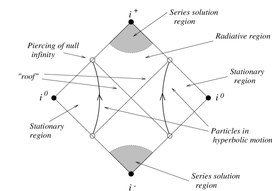
Figure 2: The different regions of a boost-rotation symmetric spacetime, including the regions of validity of the series solutions.

If the regularity of the the solutions at the poles is demanded then the leading behavior of the series is given by:

$$K_{1}=a_{0}+{\cal{O}}(w),$$ (53)

$$K_{2}=b_{0}+{\cal{O}}(w),$$ (54)

$$H_{1}=c_{0}+{\cal{O}}(w),$$ (55)

$$H_{2}=d_{0}+{\cal{O}}(w),$$ (56)

$$L=e_{0}+{\cal{O}}(w),$$ (57)

where $a_{i}$, $b_{i}$, $c_{i}$, $d_{i}$ and $e_{i}$ ($i\geq 0$) are constants. The constant $a_{0}$ can be removed using a super-translation, so that in fact $K_{1}={\cal{O}}(w)$. The asymptotic shear transforms under super-translations according to [25]:

$$\tilde{\sigma}_{2,0}(\tilde{u},x^{\alpha})=\sigma_{2,0}(\tilde{u}-\alpha,x^{\alpha})+\eth^{2}\alpha(\theta,\phi),$$ (58)

and this being so if initially one has $\sigma_{2}=-a_{0}\csc\theta+{\cal{O}}(w)$, then in order to get $\tilde{\sigma}_{2}={\cal O}(w)$ it is necessary to find a function $\alpha(\theta,\varphi)$ such that $\eth^{2}\alpha=a_{0}\csc\theta$. This is given by,

$$\alpha(\theta,\varphi)=-2a_{0}\sin\theta,$$ (59)

that despite its apparent simplicity defines a true super-translation. This choice of cuts of ${I}^{+}$ leads to the following series solutions:

$$K_{1}(w) =a_{3}\,{w^{3}}+a_{5}\,{w^{5}}+{{{\cal{O}}(w^{7})}},$$ (60)

$$K_{2}(w) =b_{3}\,{w^{3}}+b_{5}\,{w^{5}}+{{{\cal{O}}(w^{7})}},$$ (61)

$$H_{1}(w) =c_{1}\,w+\frac{3}{10\,\left({{a_{3}}^{2}}+{{b_{3}}^{2}}\right)}\left(5\,(\,b_{5}\,\left(b_{3}\,c_{1}+a_{3}\,d_{1}\right)+a_{5}\,\left(a_{3}\,c_{1}-b_{3}\,d_{1}\right))\right.$$ (62)

$$\;\;\;-\left.\left(a_{3}\,c_{1}-b_{3}\,d_{1}\right)\,\left({{c_{1}}^{2}}+{{d_{1}}^{2}}\right)\right)\,w^{3}+{{{\cal{O}}(w^{4})}},$$

$$H_{2}(w) =w\,d_{1}+\frac{3}{10\,\left({{a_{3}}^{2}}+{{b_{3}}^{2}}\right)}\left(5\,(a_{5}\,\left(b_{3}\,c_{1}+a_{3}\,d_{1}\right)-\,b_{5}\,\left(a_{3}\,c_{1}-b_{3}\,d_{1}\right))\right.$$ (63)

$$\;\;\;-\left.\left(b_{3}\,c_{1}+a_{3}\,d_{1}\right)\,\left({{c_{1}}^{2}}+{{d_{1}}^{2}}\right)\right)\,w^{3}+{{{\cal{O}}(w^{4})}},$$

$$L(w) =4\,a_{3}+\frac{2}{5}\,{{\left(30\,a_{5}-({{c_{1}}^{2}}+{{d_{1}}^{2}})\right)\,{w^{2}}}}+{{{\cal{O}}(w^{4})}}.$$ (64)

The coefficients $a_{3}$, $b_{3}$, $a_{5}$, $b_{5}$ are free parameters of the gravitational field, whereas $c_{1}$, $d_{1}$ play the same role for the electromagnetic field . In order to shorten the expressions of the components of the Weyl and Maxwell spinors, the following complex parameters will be introduced:

$$q_{1}=c_{1}+id_{1},$$ (65)

$$p_{3}=a_{3}+ib_{3},$$ (66)

$$p_{5}=a_{5}+ib_{5}.$$ (67)

With this new notation, the leading terms of the components of the Weyl spinor are found to be

$$\Psi_{4}^{1}= 6\,{\sin^{2}\theta}\left({{2\,{\bar{p}}_{3}}}\,u^{-5}+{{5\,{\bar{p}}_{5}\,{{\sin^{2}\theta}}}}\,u^{-7}\right)+{\cal O}(u^{-9}),$$ (68)

$$\Psi_{3}^{2}= -3\,{\sqrt{2}}\,\cos\theta\,\sin\theta\,\left({{2\,{\bar{p}_{3}}}}\,u^{-4}+{{5\,\bar{p}_{5}\,{{\sin^{2}\theta}}}}\,u^{-6}\right)+{\cal O}(u^{-8}),$$ (69)

$$\Psi_{2}^{3}= {{2\,\bar{p}_{3}\,\left(2-3\,\,{{\sin^{2}\theta}}\right)\,}u^{-3}}+{{{{\sin^{2}\theta}}\,\left(3\,\bar{p}_{5}\left(4-5\,\,{{\sin^{2}\theta}}\right)-\frac{2\,q_{1}\,\bar{q}_{1}}{5}\right)}}u^{-5}+{\cal O}(u^{-7}),$$ (70)

$$\Psi_{1}^{4}= 3\,{\sqrt{2}}\,\cos\theta\,\sin\theta\,\left(\bar{p}_{3}\,u^{-2}+{{\frac{1}{20}\,\left(5\,\bar{p}_{5}\left(1-5\,\cos 2\theta\right)\,+4\,q_{1}\,{\bar{q}_{1}}\right)\,u^{-4}}}\right)+{\cal O}(u^{-6}),$$ (71)

$$\Psi_{0}^{5}= 3\sin^{2}\theta\left(\,\overline{p}_{3}\,u^{-1}-\frac{1}{20}\left(5\overline{p}_{5}\left(3+5\,\cos 2\theta\right)\,-8\,q_{1}\,\bar{q}_{1}\right)u^{-3}\right)+\mbox{O}(u^{-5}),$$ (72)

$$\Psi_{0}^{6}= -\sin^{2}\theta\left(\frac{15}{2}{{\overline{p}_{3}}}-\frac{3}{8}{{\,\left(5\overline{p}_{5}\left(5+7\,\cos 2\theta\right)\,-8\,q_{1}\,\bar{q}_{1}\right)u^{-2}}}\right)+\mbox{O}(u^{-4});$$ (73)

whereas the relevant terms of the components of the Maxwell spinor are

$$\phi_{2}^{1}= q_{1}\sin\theta\left({{{u^{-3}}}}+{\frac{3}{10\,\bar{p}_{3}}{{{\sin^{2}\theta}}\,\left(5\,{p_{5}}-q_{1}\,{\bar{q}_{1}}\right)}}u^{-5}\right)+{\cal O}(u^{-7}),$$ (74)

$$\phi_{1}^{2}= -{\frac{q_{1}\cos\theta}{{\sqrt{2}}}}\left(u^{-2}-\frac{3}{10\,\bar{p}_{3}}{{{{\sin^{2}\theta}}\,\left(5\,{\bar{p}_{5}}-q_{1}\,{\bar{q}_{1}}\right)}}u^{-4}\right)+{\cal O}(u^{-6}),$$ (75)

$$\phi_{0}^{3}= -\frac{q_{1}\,\sin\theta}{2}\left(u^{-1}-\frac{1}{10\,\bar{p}_{3}}{{\left(2-3\,{{\sin^{2}\theta}}\right)\,\left(5\,{\bar{p}_{5}}-q_{1}\bar{q}_{1}\right)}}u^{-3}\right)+{\cal O}(u^{-5}),$$ (76)

$$\phi_{0}^{4}= \frac{3\,q_{1}\,\sin\theta}{4}\left(1-{\frac{1}{10\,\bar{p}_{3}}\left(4-5\,{{\sin^{2}\theta}}\right)\,\left(5\,{\bar{p}_{5}}-q_{1}\bar{q}_{1}\right)u^{-2}}\right)+{\cal O}(u^{-4}).$$ (77)

It is worth noting the existence of a peeling off property of the $u$ dependence of these coefficients:

$$\Psi_{n}^{5-n}=\mbox{O}(u^{-1-n}),$$ (78)

$$\phi_{m}^{3-m}=\mbox{O}(u^{-1-m}),$$ (79)

with $n=0,\ldots,4$ and $m=0,\ldots,2$. This behavior can be understood in the following way: one can perform a construction equivalent to the one we presented, but for past-oriented light cones, parametrized by an advanced time $v$ coordinate. The components of the Weyl and Maxwell spinors will peel off with respect to the affine parameters of the null generators of these past-oriented cones (recall that boost-rotation symmetric spacetimes are time symmetric!). Now, close to ${I}^{+}$, one can show that $r_{v}=u+\mbox{O}(u^{-1})$, where $r_{v}$ is the affine parameter in the past-oriented system. Similarly, $v\sim r$ in a neighbourhood of ${I}$, and $l^{a}$ and $n^{a}$ are “almost” parallel to $n^{a}_{v}$ and $l^{a}_{v}$ respectively. Thus, the leading coefficients should peel off with respect to $r_{v}$. Whence, they also have to peel off with $u$.

4 Asymptotic and radiative properties

We have already gathered enough information so as to study some the spacetime’s physical properties at ${I}^{+}$ in the late-time regime.

4.1 The electromagnetic charge

The total charge in the spacetime is given by

$$e=\int_{S^{2}}\phi_{1}^{2}(_{0}Y_{0,0})\mbox{d}S=\sqrt{\pi}\int_{S^{2}}\phi_{1}^{2}\sin\theta\mbox{d}\theta=O(u^{-5}),$$ (80)

i.e. it vanishes up to $O(u^{-5})$. Moreover, since the total electromagnetic charge in the spacetime is a conserved quantity, it should not contain any $u$ dependence. Therefore one can affirm that for our spacetimes

$$e=0.$$ (81)

This is in agreement with the interpretation put forward by Cornish & Utteley [11, 10], who interpreted the charged C-metric as two charged black holes of opposite charges in hyperbolic motion.

4.2 The Bondi mass and the NUT mass

Of great physical relevance is the study of the mass loss of the system due to radiative processes. This can be done by evaluating the Bondi mass, which is given by:

$$M_{B}=-\frac{1}{2}\int_{S^{2}}\mbox{Re\,}\left(\Psi_{2}^{3}+\sigma_{2}\dot{\overline{\sigma}}_{2}\right)(_{0},Y_{0,0})\mbox{d}S,$$ (82)

and can be shown to be non-increasing. Another related quantity, the NUT mass [21, 2] will also be of some interest due to the generic existence of nodal singularities in the interior of boost-rotation symmetric spacetimes [9]. The NUT mass is essentially an imaginary version of the Bondi mass:

$$M_{NUT}=-\frac{1}{2}\int_{S^{2}}\mbox{Im\,}\left(\Psi_{2}^{3}+\sigma_{2}\dot{\overline{\sigma}}_{2}\right)(_{0},Y_{0,0})\mbox{d}S,$$ (83)

The evaluation of these integrals for our solutions yields:

$$M_{B}=4\,\sqrt{\pi}\,\left(\frac{1}{15}\,{q_{1}{\bar{q}_{1}}}{{u^{-5}}}+\frac{2}{5}\,{{p_{3}\,{\bar{p}}_{3}}{{u^{-7}}}}-\frac{16}{35}\left(p_{5}\,{\bar{p}_{3}}+p_{3}\,{\bar{p}_{5}}\right)\,{{u^{-9}}}+{\frac{32}{63}\,{p_{5}\,{\bar{p}}_{5}}\,{{u^{-11}}}}\right)+{\cal O}(u^{-13})$$ (84)

$$M_{NUT}=\frac{16\sqrt{\pi}}{35}\left(p_{3}\overline{p}_{5}-\overline{p}_{3}p_{5}\right)u^{-9}+\mbox{O}(u^{-13}).$$ (85)

If the electromagnetic field is absent then,

$$M_{B}=\frac{8\sqrt{\pi}}{5}p_{3}\overline{p}_{3}\,u^{-7}+\mbox{O}(u^{-9}),$$ (86)

thus $m=p_{3}\overline{p}_{3}=|p_{3}|^{2}$ can be interpreted as the mass of the system at a fiduciary retarded time (say $u=1$). Note as well that if $u\!\longrightarrow\!\infty$ then $M_{B}\!\longrightarrow\!0$, i.e. all the mass in the spacetime is carried away. This is consistent with the standard interpretation of boost-rotation symmetric as spacetimes describing particles in hyperbolic motion. These particles eventually pierce null infinity, thus leaving the (unphysical) spacetime. Consistent with these results, Dray has shown [12] that the ADM mass of the C-metric is zero. His analysis shows that the reason for this is the particular kind of isometries this spacetime has. Therefore, it is very likely that this result also holds for the whole class of boost-rotation-symmetric spacetimes.

A similar discussion can be done with the NUT mass. The constant $g=p_{3}\overline{p}_{5}-\overline{p}_{3}p_{5}$ can be interpreted as the measure of the “strength” of the nodal singularities joining the particles in hyperbolic motion at a fiduciary time, $u=1$.

4.3 The Newman-Penrose constants

Further insight on the physical meaning of the parameters $q_{1}$ and $p_{3}$ can be achieved by looking at the Newman-Penrose constants of the gravitational and electromagnetic field.

As shown by Exton et al. [13], there will be two sets of conserved quantities for the Einstein-Maxwell system under consideration: one for the electromagnetic field only, and one for the combined electromagnetic-gravitational system. The electromagnetic NP constants are given by:

$$\mathcal{F}_{m}=\int_{S^{2}}\phi_{0}^{4}(_{1}\overline{Y}_{1,m})\,\mbox{d}S\,.$$ (87)

Note that due to the axial symmetry, all the constants, except for the one corresponding to $m=0$, will vanish identically (the $m=0$ spherical harmonic has no $\varphi$ dependence).

The NP constants for the combined gravitational-electromagnetic system are somewhat more complicated as they involve the inverse operator $\eth^{-1}$:

$$\mathcal{G}_{m}=\int_{S^{2}}\left\{\Psi_{0}^{6}+4\phi_{0}^{1}\overline{\eth}^{-1}(\overline{\phi}_{1}^{2}-\overline{E})-4\overline{E}\overline{\eth}^{-1}(\phi_{0}^{4}-F)\right\}(_{2}\overline{Y}_{2,m})\,\mbox{d}S\,,$$ (88)

where

$$E=e(_{0}Y_{0,0}),$$ (89)

$$F=\sum_{m=-1}^{1}\mathcal{F}_{m}(_{1}Y_{1,m}),$$ (90)

and

$$\overline{\eth}^{-1}(\overline{\phi}_{1}^{2}-\overline{E})=-\sum_{l=1}^{\infty}\sum_{m=-l}^{l}\frac{(_{1}Y_{l,m})}{\sqrt{l(l+1)}}\int\overline{\phi}_{1}^{2}(_{0}\overline{Y}_{l,m})\,\mbox{d}S\,,$$ (91)

$$\overline{\eth}^{-1}(\overline{\phi}_{0}^{4}-\overline{F})=-\sum_{l=2}^{\infty}\sum_{m=-l}^{l}\frac{(_{2}Y_{l,m})}{\sqrt{(l-1)(l+2)}}\int\overline{\phi}_{0}^{4}(_{1}\overline{Y}_{l,m})\,\mbox{d}S\,.$$ (92)

The spacetimes under discussion are axially symmetric, and thus they only have one nonzero complex electromagnetic and one complex gravitational NP constants (those corresponding to the $m=0$ spherical harmonics). In the region below the “roof”, the spacetime is stationary, and therefore its electromagnetic Newman-Penrose constants will be of the form (mass monopole)$\times$(electric dipole)$-$(electric charge)$\times$(mass dipole), while the gravitational constants will be of the form (mass dipole)${}^{2}-$(mass monopole)$\times$(mass quadrupole) [13].

Using equation (87) one finds that the electromagnetic NP constant is given by:

$$\mathcal{F}_{0}=\sqrt{\frac{3}{8\pi}}\,q_{1}.$$ (93)

Therefore $q_{1}$ is a product of a mass monopole and electric dipole, for there is no electromagnetic charge in the spacetime. Similarly, using equation (88) the evaluation of the gravitational NP constants yield:

$$\mathcal{G}_{0}=-6\sqrt{\frac{5}{\pi}}\,\overline{p}_{3}.$$ (94)

Thus, $p_{3}$ has to be interpreted as a quantity of quadrupolar nature, even if strictly speaking the spacetime does not has a mass monopolar moment for the particle undergoing hyperbolic motion in a boost-rotation symmetric spacetime does not always are present in pairs.

Furthermore, let us recall the formulae for radiated power for the electromagnetic and the linearized gravitational field, the so called dipole and Einstein’s quadrupole formulae [18]:

$$I_{elect}\propto\,\ddot{\bf\mbox{\bf d}}^{2},$$ (95)

$$I_{grav}\propto\,\stackrel{{\scriptstyle\ldots}}{{\mbox{\bf D}}}^{2},$$ (96)

where d is the dipolar moment of the charge distribution giving rise to the radiation field, and D is the quadrupolar moment of the mass distribution (a 3-dimensional tensor). ¿From the Bondi mass one can obtain by differentiation the flux of energy through null infinity. This is,

$$\dot{M}_{B}=-4\,\sqrt{\pi}\,\left(\frac{1}{3}\,{q_{1}{\bar{q}_{1}}}{{u^{-6}}}+\frac{14}{5}\,{{p_{3}\,{\bar{p}}_{3}}{{u^{-8}}}}\right)+\mbox{O}(u^{-10}).$$ (97)

Therefore the spacetimes under discussion radiate according to the dipole and Einstein’s quadrupole formula up to the leading terms. Higher order corrections are due to the damping of the electromagnetic field by the gravitational field, some other nonlinear effects like gravitational wave backscattering. Note as well how the flux of energy due to the gravitational field decays much faster than the flux due to the electromagnetic field. Thus at late times the main contribution to mass loss is electromagnetic in origin (Poynting vector).

4.4 Polarization states of the electromagnetic and gravitational waves

The discussion along this paper has focused on peeling electromagnetic and gravitational fields, and consequently the fields at null infinity are well defined. If one wishes to study the states of polarization of the electromagnetic or the gravitational fields, it is only necessary to consider the behavior of the type N part of the fields, that is, the leading coefficients of $\phi_{2}$ and $\Psi_{4}$ (i.e. $\phi_{2}^{1}$ and $\Psi_{4}^{1}$). The spinorial electromagnetic field is related to the components of the Maxwell field tensor via:

$$E_{1}-iB_{1}=\phi_{0}-\phi_{2}$$ (98)

$$E_{2}-iB_{2}=i(\phi_{0}+\phi_{2})$$ (99)

$$E_{3}-iB_{3}=-2\phi_{1}$$ (100)

In the case here the electromagnetic field can be seen to have two polarization states, associated with the real part and imaginary parts of $\phi_{2}^{1}$ respectively. One way to see this is to realize that if $d_{1}$ is set to zero then there will still be non vanishing components of the electromagnetic field. A similar phenomenon happens if $c_{1}$ is set to zero. This is nothing but a consequence of the existence of two different polarization states. If $\phi_{2}^{1}$ is real, then the electric and magnetic fields —see equations (98)-(100)— lie along the $e_{1}$ and $e_{2}$ directions respectively. Note that $e_{1}$ and $e_{2}$ are orthonormal vectors transverse to the null generators of outgoing light cones, explicitly:

$$e_{2}^{a}=\frac{1}{\sqrt{2}}i(m^{a}-\overline{m}^{a}),$$ (101)

$$e_{3}^{a}=\frac{1}{\sqrt{2}}(l^{a}-n^{a}).$$ (102)

Both 3-vectors are orthogonal, and have the same norm, as it should be expected from a plane wave. Let us call this polarization state $P_{x}$ (the polarization vector lies on the $e_{1}$ direction —x axis— [23]). When $\phi_{2}^{1}$ is purely imaginary ($P_{y}$ polarization), the situation gets reversed and the electric field and magnetic lie along the $e_{2}$ and $e_{1}$ directions respectively (see figure 6.3).

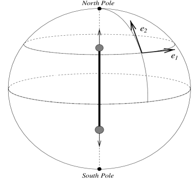
Figure 3: The directions of the polarization states of the electromagnetic and gravitational fields with respect to the celestial sphere.

By calculating the Poynting vectors for each state it can be checked that each configuration carries energy independently from the other, supporting again the assertion made on the existence of two independent degrees of freedom for the electromagnetic field.

For the gravitational field, the situation is fairly similar to that of the electromagnetic field. Again, there are two set of parameters: $\{a_{3},a_{5}\}$ (the real parts of $p_{3}$ and $p_{5}$), and $\{b_{3},b_{5}\}$ (the imaginary parts of $p_{3}$ and $p_{5}$). Both of them play an equivalent role in the expression for the Bondi mass. Hence both states of the gravitational field carry energy independently, i.e. they are true degrees of freedom (polarization states) of the gravitational field. The one associated to the real part of the Weyl tensor, which is given by the $a$-parameters, describes a $(+)$ polarization state. This can be seen by considering the geodesic deviation equation [26]:

$$\delta\ddot{x}^{a}=\frac{1}{2}\mbox{Re\,}\Psi_{4}^{1}\left(e_{2}^{a}e_{2c}-e_{1}^{a}e_{1c}\right)\delta x^{c},$$ (103)

therefore there will be tidal forces along the $e_{1}$ and $e_{2}$ directions. Similarly, if one considers the polarization state associated to the imaginary part of the Weyl tensor, one can perform a spin boost so that $\Psi_{4}$ becomes real, so that one can use again equation (103). This polarization state will be a $(\times)$ one, with tidal forces rotated $\pi/4$ with respect to the $e_{1}$ and $e_{2}$ directions.

Note that if the Killing vectors are hypersurface orthogonal, then there is only one polarization state of the gravitational field ($+$). By contrast, the electromagnetic field can always have two polarizations states, as long as $q_{1}$ is complex (a magnetic dipole moment is then present!).

4.5 Conclusions

The main objective of this paper was to construct spacetimes that could be used as examples and test bench of different techniques and ideas used in the description of on asymptotic and radiative properties of the gravitational and electromagnetic fields.

Boost-rotation symmetric spacetimes are regarded as the best suited candidates for such a test bench since they contain the only examples known up to date of asymptotically flat radiative exact solutions. Perhaps the most remarkable result was that of showing how the Newman-Penrose constants allow one to consider, at least up to quadrupoles, multipolar moments of non-stationary spacetimes without having to resort to the linearized theory (cfr. the results on the mass loss). As seen, the complexity of the equations involved precludes the obtention of nice closed expressions; however, the asymptotic expressions for late times have allowed to extract most of physical properties of interest; this regardless of the natural limitations that this approach carries.

References

- [1] A. Ashtekar & T. Dray, On the existence of solutions to Einstein’s field equations with non-zero Bondi news, Comm. Math. Phys. 79, 581 (1981).
- [2] A. Ashtekar & A. Sen, NUT 4-momenta are forever, J. Math. Phys. 23, 2168 (1982).
- [3] J. Bičák, Gravitational radiation from uniformly accelerated particles in general relativity, Proc. Roy. Soc. Lond. A 302, 201 (1968).
- [4] J. Bičák, C. Hoenselaers, & B. G. Schmidt, The solutions of the Einstein equations for uniformly accelerated particles without nodal singularities. I. Freely falling particles in external fields, Proc. Roy. Soc. Lond. A 390, 397 (1983).
- [5] J. Bičák, C. Hoenselaers, & B. G. Schmidt, The solutions of the Einstein equations for uniformly accelerated particles without nodal singularities. II. Self-accelerating particles, Proc. Roy. Soc. Lond. A 390, 411 (1983).
- [6] J. Bičák & A. Pravdová, Symmetries of asymptotically flat electrovacuum space-times and radiation, J. Math. Phys. 39, 6011 (1998).
- [7] J. Bičák & A. Pravdová, Axisymmetric electrovacuum spacetimes with a translational Killing vector at null infinity, Class. Quantum Grav. 16, 2023 (1999).
- [8] J. Bičák & B. G. Schmidt, Isometries compatible with gravitational radiation, J. Math. Phys. 25, 600 (1984).
- [9] J. Bičák & B. G. Schmidt, Asymptotically flat radiative space-times with boost-rotation symmetry: the general structure, Phys. Rev. D 40, 1827 (1989).
- [10] F. H. J. Cornish & W. J. Uttley, The interpretation of the C metric. The charged case when , Gen. Rel. Grav. 27, 735 (1995).
- [11] F. H. J. Cornish & W. J. Uttley, The interpretation of the C metric. The vacuum case, Gen. Rel. Grav. 27, 439 (1995).
- [12] T. Dray, On the asymptotic flatness of the C metrics at spatial infinity, Gen. Rel. Grav. 14, 109 (1982).
- [13] A. R. Exton, E. T. Newman, & R. Penrose, Conserved quantites in the Einstein-Maxwell theory, J. Math. Phys. 10, 1566 (1969).
- [14] H. Farhoosh & R. L. Zimmerman, Killing horizons and dragging of the inertial frame about a uniformly accelerating particle, Phys. Rev. D 21, 317 (1980).
- [15] H. Farhoosh & R. L. Zimmerman, Surfaces of infinite red-shift around a uniformly accelerating and rotating particle, Phys. Rev. D 21, 2064 (1980).
- [16] W. Kinnersley & M. Walker, Uniformly accelerating charged mass in general relativity, Phys. Rev. D 2, 1359 (1970).
- [17] D. Kramer, H. Stephani, E. Herlt, & M.MacCallum, Exact solutions of Einstein’s field equations, Cambridge University Press, 1980.
- [18] L. D. Landau & E. M. Lifshitz, The classical theory of fields, Pergamon Press, 1951.
- [19] R. Penrose & W. Rindler, Spinors and space-time. Volume 2. Spinor and twistor methods in space-time geometry, Cambridge University Press, 1986.
- [20] J. F. Plebanski & M. Demianski, Rotating, charged and uniformly accelerating mass in general relativity, Ann. Phys. 98, 98 (1976).
- [21] S. Rawasami & A. Sen, Dual-mass in general relativity, J. Math. Phys. 22, 2612 (1981).
- [22] F. Schwarz, Equivalence classes and symmetries of Abel’s equation, J. Symb. Comp 11, 1 (1999).
- [23] H. Stephani, General Relativity, Cambridge University Press, 1982.
- [24] H. Stephani, Differential equations: their solution using symmetires, Cambridge University Press, 1989.
- [25] J. Stewart, Advanced general relativity, Cambridge University Press, 1991.
- [26] P. Szekeres, The gravitational compass, J. Math. Phys. 6, 1387 (1965).
- [27] J. A. Valiente Kroon, On Killing vector fields and Newman-Penrose constants, J. Math. Phys. 41, 898 (2000).