Close limit of grazing black hole collisions:
non-spinning holes

Abstract

Using approximate techniques we study the final moments of the collision of two (individually non-spinnning) black holes which inspiral into each other. The approximation is based on treating the whole space-time as a single distorted black hole. We obtain estimates for the radiated energy, angular momentum and waveforms for the gravitational waves produced in such a collision. The results can be of interest for analyzing the data that will be forthcoming from gravitational wave interferometric detectors, like the LIGO, GEO, LISA, VIRGO and TAMA projects.

I Introduction

The phrase “collision of black holes” has an aura of a mysterious and exotic happening that is not far from the reality of such an event. A black hole is not an ordinary object defined by the amount and properties of the material of which it is made. Rather it is a region from which no signal can escape. The surface, the black hole horizon, bounding this region is defined by the formal “no escape” property. Unlike the surface of an ordinary object the horizon has no local properties that would be sensed by an observer with the bad fortune to fall inward through it. A collision of two holes is the process in which two no-escape regions merge to become a single, larger, region of no escape. In the last few years such mergers have become the focus of much research attention, for two not entirely independent reasons.

The first reason is the development of numerical relativity [1]. General relativity, Einstein’s theory of gravity, sets the dynamics of space-time via a set of nonlinear partial differential equations of such complexity that analytic solutions have been limited to two classes: solutions of high symmetry, or solutions based on approximation techniques, such as linearized weak field theory. The study of Einstein’s equations on computers has been viewed as the key to finding more general asymmetric strong field solutions and it was natural for this key to be be applied to black hole collisions. Black holes are incontrovertibly strong field regions, but single isolated black holes are stationary solutions of Einstein’s theory, and the simplifying symmetry of time independence allows for closed form well-understood solutions [2]. Collisions of black holes, on the other hand, are necessarily nonstationary as well as being crucially strong-field events. It is known that the collision will result in a single final black hole and in the generation of gravitational waves carrying off some of the mass energy originally associated with the holes. But this is all that is known with certainty. The nature of the merging of the horizons, in the general collision, is not even qualitatively understood.

A reasonably complete understanding awaits progress in numerical relativity, and the wait has been longer than anticipated. The solution of general black hole collisions on computers has proved to be remarkably difficult. There is, however, a class of cases in which reliable answers are available. If the collision is a ’head-on’ collision along a straight line, then there is rotational symmetry about the line of the collision. Though the collision is still highly dynamic and nonlinear, the simplifications afforded by this symmetry reduce the computational demands sufficiently that the collision could successfully be simulated even in the mid 1970’s, and run with good reliability in the mid 1990’s[3]. The simplification of head-on collisions, however, masks some of the physics of the most interesting types of collisions, the fully three dimensional collisions at the end point of the inspiral of a mutually orbiting pair of black holes.

The second development that directed attention to black hole collisions is the advent of sensitive gravitational wave detectors. In the next few years, several interferometric gravitational wave observatories (the LIGO project in the US, the VIRGO and GEO projects in Europe and the TAMA project in Japan [4]) may be capable of detecting gravitational waves. Whether near term searches are successful will depend more than anything else on the strength of astrophysical sources. Attributes of a good generator of gravitational waves include strong gravitational fields and high velocities, so black hole processes are a natural source to consider. It is astrophysically plausible that black holes form binary associations with other objects, including other black holes [5]. Due to the loss of energy by the emission of gravitational radiation, the separation and period of the binary orbits would decrease. If the binary consists of two black holes, the inspiral would end with a rapid strong field merger that has the potential to be a powerful source of detectable gravitational waves [6].

The whole process of inspiral generates gravitational radiation, but in the early large-separation stages the radiation is relatively weak and is reasonably well described by Newtonian gravity theory and Post-Newtonian extensions of it [7]. It is only the final strong field merger that could in principle produce a powerful burst of gravitational waves, but at this point only one parameter of the burst is reliably known. The characteristic frequency of the waves is inversely proportional to the mass of the final black hole formed, and works out to be on the order of $10^{3}$ Hz for a 10$M_{\odot}$ hole, a typical expected mass of a “stellar” sized hole. For supermassive holes of mass $\geq 10^{6}M_{\odot}$ typical of galactic nuclei, the waves would be less than 1 Hz. The maximum sensitivity of the next generation of gravitational wave detectors occurs at frequency around 100 Hz and the detectors will be ideally suited to waves from a black hole with mass of several hundred $M_{\odot}$. Some recent observations[8] offer indirect evidence that black holes in this range may exist. If they do not, then the detection of the collision of black holes may require the deployment of space-based detectors[9] sensitive to the low frequency waves produced by supermassive holes.

The ratio of the masses in a binary determines both how difficult it is to analyze, and how exciting it is as a potential source. If the mass of a black hole $M_{1}$ is much larger than the mass of its binary companion $M_{2}$, then the smaller mass object can be treated as a perturbation to the well understood spacetime of the larger mass black hole. The equations that describe perturbations are linear, and hence relatively easily dealt with in general. In the specific case of perturbations to black hole spacetimes, the techniques of calculation were worked out in the 1970s and resulted in the Regge-Wheeler and Zerilli equations [10, 11] for perturbations of Schwarzschild (nonrotating) black holes, and in the Teukolsky [12] equation for perturbations of Kerr (rotating) black holes. The relatively easily analyzed [13] “particle limit” case $M_{2}\ll M_{1}$ may be of interest in connection, say, with neutron stars merging with supermassive black holes, but this process cannot give the hoped for high power. It is easy to show the gravitational wave power generated scales in the masses as $(M_{2}/M_{1})^{2}$. High power requires roughly equal masses, and this means the simplifications of the particle limit do not apply to the most interesting sources.

If not directly applicable to equal mass inspiral, the clarity of the particle limit can, at least, help us to formulate questions about the nature of the endpoint of inspiral, like the existence of a last stable circular orbit. As a particle orbits a black hole it reaches a radius at which it can no longer stably orbit with slowly decreasing radius and it begins a rapid inward plunge. For the inspiral of two roughly equal mass holes it can be imagined that the binary gradually spirals inward or that it reaches a point at which a discontinuous plunge begins. If the late orbits are being degraded rapidly enough by the emission of gravitational radiation, there might not even be any meaning to late stage “stability.” This uncertainty about even the qualitative nature of the late stage of the inspiral is related to an important, but totally unresolved, question: How does the inspiraling binary shed enough angular momentum to form a black hole? In a relativist’s units in which $c=G=1$, a black hole must have a total angular momentum $J$ that is limited by the maximum angular momentum $J=M^{2}$ that a rotating (Kerr) black hole can possess. Until the binary pair is close, its angular momentum will be above this limit, but technical considerations[14] limit the rate at which angular momentum can be shed in gravitational waves at very late stages. If both black holes of the pair are rapidly rotating with angular momentum in the same direction the shedding appears to present a barrier to the formation of the final single black hole. It is possible that even the qualitative details of the late stage inspiral depend on the angular momentum of the inspiraling binary.

The set of possibilities is considerable and the answers are important both to our understanding of nonlinear gravitational interactions and to an understanding of gravitational wave sources. Real answers will require advances in numerical relativity that will be several years in coming, but interest in the questions justifies approximation methods that can help, even slightly, to close some of the wide open questions. We take such an approach here. We offer an estimate of the gravitational radiation generated during the late stage of inspiral of two black holes. Our method involves a number of assumptions and limitations that constrain its applicability and reliability, but for all its shortcomings it is one step towards a complete understanding.

The approximation method we use, the “close limit,” [15] takes advantage of the property of a black hole horizon. Late in the merger of the binary the single horizon of the final black hole engulfs the entire binary. All the complex structure of the binary will be inside that final horizon, and cannot influence spacetime outside the horizon. It is only what is outside the horizon that can generate gravitational waves that can be detected by distant observers. Since the ultimate fate of the merger is a stationary black hole, it follows that sufficiently late in the merger what is outside the hole will be a perturbation of the final stationary hole. Thus the gravitational waves generated during the latest stage of inspiral can be computed using the techniques of perturbations of black hole spacetimes, with the Zerilli, Regge-Wheeler, and Teukolsky equations.

To understand how the close limit method is to be used, it is necessary to consider the general problem addressed by numerical relativity. Einstein’s field equations are divided into “initial value” equations and equations of time evolution [16]. The initial value equations determine the nature of spacetime at a chosen initial moment. The solutions of these initial value equations are the initial values for the remaining differential equations of Einstein’s theory, the equations that determine the spacetime (including its gravitational wave content) to the future of the initial time. The two tasks of numerical relativity are first to find an initial value solution representing a moment in the life of the colliding holes, and second to find the future spacetime for those initial values. The more computationally difficult task is that of evolving to the future and the codes that accomplish this task tend to be unstable for long time evolutions. For long evolutions to be avoided, the initial value solutions must be chosen to be a moment late in the life of the inspiral. If that moment is late enough, the close limit method can be brought to bear and evolution can be carried out with the stable linearized equations of perturbation theory. But choosing too late a starting moment for evolution creates a new difficulty.

The connection of an initial value solution to a “sensible” physical configuration for the binary is reasonably secure only if the binary pair is well separated. At close separations, the gravitational field of each of the binary holes strongly affects the other hole, and the individual mass, individual angular momentum, and physical separation of the holes lose clear meaning. The problem then requires navigating between the Scylla of numerical instabilities for evolution, and the Charybdis of uncertain initial conditions. By using a very late initial moment and linearized evolution, the close limit method completely avoids the former hazard.

There are reasons beyond speculation to believe that close limit evolutions give useful answers. Numerical relativity results are available for axisymmetric head-on collisions[3]. These represent evolution of a number of initial value solutions, in particular the closed form solution due to Misner[17], containing a single parameter representing the initial separation of equal mass holes in units of the mass of the spacetime (in $c=G=1$ units). This separation index defines a parameterized family of initial value solutions. Choices of this parameter can be made corresponding to large or small initial separation. When numerical relativity and close limit results are compared it is seen that agreement is excellent for small initial separations, and is surprisingly good even when the initial configuration is not close enough for a horizon to engulf the entire binary[18, 19]. Arguments can be made also, that the gravitational waves calculated in the late stage of inspiral are not highly sensitive to details of initial data. Particularly interesting in this regard is work by Abrahams and Cook[20].

In the past several years the close limit method has been extensively studied for head-on collisions of boosted and spinning holes and compared with the results of numerical relativity. Most notably, second order perturbation theory has been developed for the close limit method[21]. In this process of comparison much has been learned about the strengths and limitations of the close limit method, with the goal of applying the method to problems that cannot yet be handled with numerical relativity. The present work represents the first example of this. We report here the results of the application of the close limit method for the three dimensional problem of the late stage inspiral of two black holes.

We will use the close limit method for the initial data families constructed by the Bowen and York [22] method and the associated “punctures” families [23]. It is known that these families possess an artificial radiation content when one considers black holes that are close, but such content is also known to be moderate [24]. An important advantage of these methods is that they are typically the starting point for numerical relativity, and thus close limit evolution of these starting points can be compared with the numerical evolution of these same initial data when such evolutions become available. The most important disadvantage, for our purposes, is that the Bowen-York family does not include the Kerr solution, the solution for a rotating hole. This precludes finding a family of initial value solutions that goes, in the limit of small initial separation, to a Kerr black hole. With Bowen-York initial value solutions, then, we cannot consider a collision that will result in a rapidly rotating hole. Rather, we limit our attention to collisions involving a modest amount of total angular momentum and consider the angular momentum as well as the initial separation to be a perturbation of a nonrotating final hole. It it should also be mentioned that currently fashionable astrophysical scenarios suggest that the individual holes might not carry a significant amount of spin [5] in realistic black hole collisions.

The organization of this paper is as follows: in the next section we review the method for obtaining the initial data and describe the approximations involved. In the following two sections we discuss how to set up the perturbative formalism geared towards evolution. Since the collisions have net angular momentum we will evolve them both as a perturbation of a rotating and a non-rotating black hole. The comparison of both approaches is given in the subsequent section and we will see that insight is gained by treating the problem in two different ways. We end with a discussion of the results in terms of waveforms and radiated energies and we describe a puzzle in the calculation of the angular momentum radiated.

For the reader who wishes to be spared all the details, we summarize our results in a brief punchline: the final ringdown of the inspiraling collision of two non-spinning black holes is unlikely to radiate more than $1\%$ of the mass of the system or more than $0.1\%$ of its angular momentum in gravitational waves.

II Initial data

To evolve a spacetime in general relativity, one needs to provide initial data, a 3-geometry $g_{ab}$ and an extrinsic curvature $K_{ab}$, that solve Einstein’s equations on some starting hypersurface (i.e., at some starting time). For two black holes, this is an easy task if the holes are far apart, since one can superpose the solutions for two individual holes ignoring their interactions. When the black holes are close on the initial hypersurface, the astrophysically correct initial data is the solution corresponding to what would have evolved during the binary inspiral, but such an evolution cannot be computed with present day techniques. One must therefore use a somewhat artificial initial data solution that is a best guess at a representation of close black holes. The need for such a guess is one of the sources of uncertainty in our result.

A Summary of the Bowen–York construction:

The initial value equations for general relativity are,

$$\nabla^{a}(K_{ab}-g_{ab}K) = 0$$ (1)

$${}^{3}R-K_{ab}K^{ab}+K^{2} = 0$$ (2)

where $g_{ab}$ is the spatial metric, $K_{ab}$ is the extrinsic curvature and ${}^{3}R$ is the scalar curvature of the three metric. If we propose a 3-metric that is conformally flat $g_{ab}=\phi^{4}\widehat{g}_{ab}$, with $\widehat{g}_{ab}$ a flat metric, and $\phi^{4}$ the conformal factor, and we use a decomposition of the extrinsic curvature $K_{ab}=\phi^{-2}\widehat{K}_{ab}$, and assume maximal slicing $K_{a}^{a}=0$, the constraints become,

$$\widehat{\nabla}^{a}\widehat{K}_{ab} = 0$$ (3)

$$\widehat{\nabla}^{2}\phi = -\frac{1}{8}\phi^{-7}\widehat{K}_{ab}\widehat{K}^{ab}\ ,$$ (4)

where $\widehat{\nabla}$ is a flat-space covariant derivative.

To solve the momentum constraint, we start with a solution that represents a single hole with linear momentum $P$ [25],

$$\hat{K}^{\rm one}_{ab}={3\over 2r^{2}}\left[2P_{(a}n_{b)}-(\delta_{ab}-n_{a}n_{b})P^{c}n_{c}\right]\ .$$ (5)

In this expression for the conformally related extrinsic curvature at some point $x^{a}$, the quantity $n_{b}$ is a unit vector, in the “base” flat space with metric $\hat{g}_{ab}$, directed from a point representing the location of the hole to the point $x^{a}$. The symbol $r$ represents the distance, in the flat base space, from the point of the hole to $x^{a}$. It is straightforward to show that the solution of the Hamiltonian constraint corresponding to eq. (5) corresponds to a spacetime with ADM momentum $P_{a}$.

The next step is to modify this to represent holes centered at $x=\pm L/2$ in the conformally flat metric. Since the momentum constraint is linear, we can simply add two expressions of the above form,

$$\widehat{K}^{\rm two}_{ab}=\widehat{K}^{\rm one}_{ab}\left(x\rightarrow x-L/2,{P_{y}=P}\right)+\widehat{K}^{\rm one}_{ab}\left(x\rightarrow x+L/2,{P_{y}}=-P\right)\ .$$ (6)

We will choose in further expressions to use a polar coordinate system in the flat space determined by $\hat{g}_{ab}$ centered in the mid-point separating the two holes and label the polar coordinates as $(R,\theta,\phi)$. So $R$ will be the distance in the flat space from the midpoint between the holes.

To solve the Hamiltonian constraint 4, we introduce an approximation, (the slow approximation) which we will show is enough for our purposes. In fact, in this approximation the solution for the conformal factor turns out to be the familiar Misner [17] solution if one chooses the topology of the slice to have a single asymptotically flat region, or the Brill–Lindquist [26] solution if there are three asymptotically flat regions.

B The slow approximation

We assume that the black holes are initially close, and that the initial momentum $P$ is small. We denote by $\vec{n}^{+}$ and $\vec{n}^{-}$ the normal vectors corresponding, respectively, to the one hole solutions at $x=+L/2$ and at $x=-L/2$, and we define $R$ to be the distance to a field point, in the flat conformal space, from the point midway between the holes. For large $R$, the normal vectors $\vec{n}^{+}$ and $\vec{n}^{-}$ almost cancel. More specifically $\vec{n}^{+}=-\vec{n}^{-}+O(L/R)$. A consequence of this is that the total initial $\widehat{K}^{ab}$ is first order in $L/R$, and its ($R,\theta,\varphi$ coordinate basis) components can be written as

$$\hat{K}_{ab}={3PL\over 8R^{3}}\left[\begin{array}[]{ccc}8\sin^{2}\theta\sin 2\varphi&0&8R\sin^{2}\theta\\ 0&R^{2}(-5+\cos 2\theta)\sin 2\varphi&-2R^{2}\sin 2\varphi\sin 2\theta\\ 8R\sin^{2}\theta&-2R^{2}\sin 2\varphi\sin 2\theta&R^{2}\sin^{2}\theta\sin 2\varphi(1+3\cos 2\theta)\end{array}\right]\ .$$ (7)

This solution for $\hat{K}_{ab}$ is first order, both in $P$ and $L$. Thus the source term in the Hamiltonian constraint is quadratic in $P$. If we choose to find a solution to the conformal factor to first order in $P$ (which should give us a good approximation in the case of slowly moving holes), we can ignore this quadratic source term. So now, the Hamiltonian constraint looks like the one for zero momentum, which is simply the Laplace equation. A well known solution to this, is the Misner solution [17]. This solution, is characterized by a parameter $\mu_{0}$ which describes the separation of the two throats. We can relate this parameter to the conformal distance $L$ in the following way [3],

$$L/M=\frac{\rm{\coth}\mu_{0}}{2\Sigma_{1}}\ \ \hskip 30.0pt\ \ \ \Sigma_{1}\equiv\sum_{n=1}\frac{1}{\sinh n\mu_{0}}\ .$$ (8)

To clarify: in the slow approximation we are considering, the data we use in our simulations consists of the extrinsic curvature proposed by Bowen and York and the conformal factor due to Misner. This might appear as odd, since the conformal factor of Misner is “symmetrized” through the throats and the extrinsic curvature due to Bowen and York is not. What we do is not inconsistent, it is just a different (and perhaps from a certain point of view less natural) choice of boundary conditions for the fields. In practice, in the close limit and to first order in perturbation theory, the conformal factor of Misner differs from that of Brill and Lindquist by a numerical factor that can be absorbed in the definition of the separation of the holes [27].

Some readers may be disturbed by the slow approximation, since in the computation of certain quantities, for instance the ADM mass, the higher order terms in the expansion in terms of the momentum are crucial. We have already discussed this in detail in previous head-on simulations [28]. The bottomline is that to get an accurate estimate of the ADM mass for high values of the momentum one indeed needs a full solution of the Hamiltonian constraint and not a “slow approximation” solution. For the values of the separations and the momenta we will consider in this paper ($a<0.5$) the ADM mass computed with the slow approximation and the one computed with the full solution differ by less than $10\%$ so we will ignore this difference.

We must now map the coordinates of the initial value solution to the coordinates for the Schwarzschild/Kerr (in the vanishing spin limit) background. To do this, we interpret the $R$ as the isotropic radial coordinate of a Schwarzschild spacetime, and we relate it to the usual Schwarzschild radial coordinate $r$ by $R=(\sqrt{r}+\sqrt{r-2M})^{2}/4$. From this we arrive at the following expression for the components of the extrinsic curvature,

$$K_{ab}={3PL\over 8r^{3}}\left[\begin{array}[]{ccc}\frac{8\sin^{2}\theta\sin 2\varphi}{1-2M/r}&0&\frac{8r\sin^{2}\theta}{\sqrt{1-2M/r}}\\ 0&r^{2}(-5+\cos 2\theta)\sin 2\varphi&-2r^{2}\sin 2\varphi\sin 2\theta\\ \frac{8r\sin^{2}\theta}{\sqrt{1-2M/r}}&-2r^{2}\sin 2\varphi\sin 2\theta&r^{2}\sin^{2}\theta\sin 2\varphi(1+3\cos 2\theta)\end{array}\right]\ .$$ (9)

Here we have used the fact that

$$\phi^{2}\approx\phi_{\rm Mis}^{2}\approx\phi_{\rm Schw}^{2}=r/R=\frac{1}{\sqrt{1-2M/r}}\,\frac{dr}{dR}\ .$$ (10)

III The close limit as a perturbation of a Schwarzschild hole

In this paper we will evolve the initial data we just constructed using the perturbative evolution equations for linearized first order perturbations: the Zerilli equation in the case of a Schwarzschild background and the Teukolsky equation in the case of a Kerr background. We need to construct the initial data for these equations in terms of the metric and extrinsic curvature we discussed above. In this section we discuss the setup of initial data and evolution of the problem as a perturbation of a Schwarzschild black hole, using the Zerilli–Regge–Wheeler formalism.

A Setting up the initial data for the Zerilli function

Given the three metric and the extrinsic curvature, one can explicitly construct the zeroth and first order term of a power series expansion in a fiducial time variable $t$ of the space-time metric. From this expression one can read off the appropriate coefficients of the multipolar expansion of the metric in the Regge–Wheeler [10] notation. The only nonvanishing perturbations at $t=0$ are,

$$H_{2}[\ell=2,m=\pm 2] = K[\ell=2,m=\pm 2]=\sqrt{{6\pi\over 5}}{8ML^{2}\over\sqrt{r}(\sqrt{r}+\sqrt{r-2M})^{5}}$$ (11)

$$H_{2}[\ell=2,m=0] = K[\ell=2,m=0]=-2\sqrt{{\pi\over 5}}{8ML^{2}\over\sqrt{r}(\sqrt{r}+\sqrt{r-2M})^{5}}$$ (12)

We compute the time derivative of these quantities, using the extrinsic curvature $K_{ij}$ obtained in the last section. The nonvanishing ones are,

$${\partial H_{2}[\ell=2,m=-2]\over\partial t} = -i24\sqrt{{\pi\over 30}}PL{\sqrt{r-2M}\over r^{3}\sqrt{r}}$$ (13)

$${\partial H_{2}[\ell=2,m=2]\over\partial t} = -{\partial H_{2}[\ell=2,m=-2]\over\partial t}$$ (14)

$${\partial K[\ell=2,m=-2]\over\partial t} = i\sqrt{30\pi}PL{\sqrt{r-2M}\over r^{3}\sqrt{r}}$$ (15)

$${\partial K[\ell=2,m=2]\over\partial t} = -{\partial K[\ell=2,m=-2]\over\partial t}$$ (16)

$${\partial G[\ell=2,m=-2]\over\partial t} = i\sqrt{{6\pi\over 5}}PL{\sqrt{r-2M}\over r^{3}\sqrt{r}}$$ (17)

$${\partial G[\ell=2,m=2]\over\partial t} = -{\partial G[\ell=2,m=-2]\over\partial t}$$ (18)

where $i$ is the imaginary unit. (Here we are using the standard conventions for the spherical harmonics. Notice that the $m=2$ and $m=-2$ perturbations are individually complex, but when they are added to give the total perturbation the resulting function of $t,r,\theta$ and $\varphi$ is real, as of course it must be.

We also have an odd parity contribution,

$${\partial{\ }^{\mbox{{odd}}}h_{1}[\ell=1,m=0]\over\partial t}=8\sqrt{3\pi}{PL\over r^{2}}.$$ (19)

This perturbation represents the difference between the Kerr solution that represents the rotating space-time and the Schwarzschild background used in the perturbative approach. To first order it decouples from all other perturbations, and in fact is unchanging in time, corresponding to the conservation of angular momentum to first order in the perturbations. The change over time in the quantity induced by second order perturbations, will be discussed below in connection with the radiation of angular momentum.

The Zerilli function is defined by (see for instance [30]),

$$\psi_{(\ell,m)} = {2r(r-2M)\over\ell(\ell+1)(\lambda r+3M)}\left[{{H}_{2}}_{(\ell,m)}-r\frac{\partial{K}_{(\ell,m)}}{\partial r}-\frac{r-3M}{r-2M}{K}_{(\ell,m)}\right]$$ (21)

$$+{r^{2}\over\lambda r+3M}\left[{K}_{(\ell,m)}+(r-2M)\left({\partial{G}_{(\ell,m)}\over\partial r}-{2\over r^{2}}{{h}_{1}}_{(\ell,m)}\right)\right].$$

Therefore, for $t=0$ we have

$$\psi_{(2,m)}(0,r)={r(r-2M)\over 3(2r+3M)}\left[{{H}_{2}}_{(2,m)}(0,r)-r{\partial{K}_{(2,m)}(0,r)\over\partial r}\right]+{r\over 3}{K}_{(2,2)}(0,r).$$ (22)

and

$$\dot{\psi}_{(2,m)}(0,r) = {r(r-2M)\over 3(2r+3M)}\left[{\dot{H_{2}}}_{(2,m)}(0,r)-r{\partial\dot{K}_{(2,m)}(0,r)\over\partial r}+3r{\partial\dot{G}_{(2,m)}\over\partial r}\right]$$ (24)

$$+{r\over 3}\dot{K}_{(2,2)}(0,r).$$

After some simplifications we have the initial data for the Zerilli function,

$$\psi_{(2,2)}(0,r)=4\sqrt{{2\pi\over 15}}ML^{2}{r\;(7\sqrt{r}+5\sqrt{r-2M})\over(2r+3M)(\sqrt{r}+\sqrt{r-2M})^{5}}$$ (25)

and

$$\dot{\psi}_{(2,2)}(0,r)=-{i\sqrt{30\pi}\over 5}PL{(4r+3M)\sqrt{r-2M}\over r^{5/2}(2r+3M)}$$ (26)

and the Zerilli function for $(\ell=2,m=-2)$ is the complex conjugate of $\psi_{(2,2)}(t,r)$. The initial data for the $\ell=2,m=0$ Zerilli function is

$$\psi_{(2,0)}(0,r) = -{8\over 3}\sqrt{\pi\over 5}{ML^{2}r\;(7\sqrt{r}+5\sqrt{r-2M})\over(2r+3M)(\sqrt{r}+\sqrt{r-2M})^{5}}$$ (27)

$$\dot{\psi}_{(2,0)}(0,r) = 0.$$ (28)

B Evolution of the Zerilli function and computation of physical quantities

Given the Cauchy data from the last section, the time evolution is obtained from the Zerilli equation [30],

$$-{\partial^{2}\psi_{(\ell,m)}\over\partial t^{2}}+{\partial^{2}\psi_{(\ell,m)}\over\partial r_{*}^{2}}+V(r_{*})\psi_{(\ell,m)}=0,$$ (29)

where $V(r_{*})$ is the ($m$-independent) Zerilli potential,

$$V(r_{*})=2\left(1-{2M\over r}\right){\lambda^{2}r^{2}\left[(\lambda+1)r+3M\right]+9M^{2}(\lambda r+M)\over r^{3}(\lambda r+3M)^{2}}\ ,$$ (30)

where $\lambda={(\ell-1)(\ell+2)}/{2}$ and $r_{*}=r+2M\ln(r/2M-1)$.

We need to establish a convenient formula for the radiated energy, similar to that present in [31] but applied to the non-axisymmetric case. We start from the expression of the radiated energy computed via the Landau–Lifshitz pseudo-tensor following the notation and derivations of [31],

$${d{\rm Power}\over d\Omega}=\lim_{r\rightarrow\infty}{1\over 16\pi r^{2}}\left[\left({\dot{h}_{\theta\phi}\over\sin\theta}\right)^{2}+{1\over 4}\left(\dot{h}_{\theta\theta}-{1\over\sin^{2}\theta}\dot{h}_{\phi\phi}\right)^{2}\right],$$ (31)

and translating to the Regge–Wheeler notation and integrating on solid angles we get,

$${\rm Power}={3\over 16\pi}\left[2\left|\dot{\psi}_{(2,0)}\right|^{2}+4\left|\dot{\psi}_{(2,2)}\right|^{2}\right]$$ (32)

and one can obtain the radiated energy integrating over time. The power naturally comes out in units of the mass of the background spacetime.

To compute the radiated angular momentum one could also start by considering the Landau–Lifshitz pseudo-tensor and construct and asymptotic expression for angular momentum flux. This approach was pursued, for instance, in [32] to compute expressions for the radiation of angular momentum in terms of multipoles. An alternative approach is to simply compute the change in the angular momentum of the spacetime, which we characterize to linear order in perturbation theory through the function,

$$r^{2}{\ }^{\mbox{{odd}}}h_{0},_{r}(r,t)-2r{\ }^{\mbox{{odd}}}h_{0}(r,t)r^{2}-{\ }^{\mbox{{odd}}}h_{1},_{t}(r,t).$$ (33)

This is a first order gauge invariant if ${\ }^{\mbox{{odd}}}h_{0}$, and ${\ }^{\mbox{{odd}}}h_{1}$ are first order perturbations. Moreover, for $\ell=1,m=0$, this gauge invariant is constant, equal to $4\sqrt{3\pi}J$, where $J$ is the total angular momentum, if the perturbations are axially symmetric.

If we look at second order perturbations we find

$${\partial\over\partial t}\left[r^{2}{\ }^{\mbox{{odd}}}h_{0},_{r}(r,t)-2r{\ }^{\mbox{{odd}}}h_{0}(r,t)-r^{2}{\ }^{\mbox{{odd}}}h_{1},_{t}(r,t)\right]={\cal{S}}_{\mbox{Jdot}}$$ (34)

where ${\cal{S}}_{\mbox{Jdot}}$ is a ‘source’, quadratic in first order perturbations.

Therefore the change in angular momentum, due to radiation may be obtained by integrating ${\cal{S}}_{\mbox{Jdot}}$ for all $t$ (or from $t=0$ to $t=\infty$, it makes no difference), in the limit $r\rightarrow\infty$. After several simplifications and cancelling terms that result from integration by parts, we end up with

$$\Delta J={3i\over 4\pi}\lim_{r\rightarrow\infty}\int_{0}^{\infty}\left[\psi_{(2,-2)}(r,t){\partial\psi_{(2,2)}(r,t)\over\partial t}-\psi_{(2,2)}(r,t){\partial\psi_{(2,-2)}(r,t)\over\partial t}\right]dt$$ (35)

If we write

$$\psi_{(2,2)}(r,t)=\mbox{Re}(\psi)+i\mbox{Im}(\psi)$$ (36)

we have

$$\psi_{(2,2)}(r,t)=\mbox{Re}(\psi)-i\mbox{Im}(\psi)$$ (37)

and we find

$$\Delta J={3\over 2\pi}\lim_{r\rightarrow\infty}\int_{0}^{\infty}\left[\mbox{Im}(\psi){\partial\mbox{Re}(\psi)\over\partial t}-\mbox{Re}(\psi){\partial\mbox{Im}(\psi)\over\partial t}\right]dt.$$ (38)

We have checked by explicit substitution that this form coincides with the results from the flux formulas of Thorne [32]. It reassures our confidence in the consistency of the Regge–Wheeler–Zerilli perturbative formalism to notice that the changes to second order are in accordance with the first order flux.

IV Evolution as a perturbation of a Kerr black hole

To treat the problem as a perturbation of a Kerr black hole we need to set up initial data and evolve the Teukolsky equation. The formalism for setting up initial data in terms of Cauchy metric data was developed in [33], we only give a brief sketch here and refer the reader to that paper for further details.

The relevant Weyl scalar for gravitational radiation is

$$\psi_{4}=-C_{\alpha\beta\gamma\delta}n^{\alpha}\overline{m}^{\beta}n^{\gamma}\overline{m}^{\delta},$$ (39)

since it is directly related to outgoing gravitational waves. We can rewrite this as

$$-\psi_{4}=R_{ijkl}n^{i}\overline{m}^{j}n^{k}\overline{m}^{l}+4R_{0jkl}n^{[0}\overline{m}^{j]}n^{k}\overline{m}^{l}+4R_{0j0l}n^{[0}\overline{m}^{j]}n^{[0}\overline{m}^{l]},$$ (40)

which in turn can be written in terms of hypersurface quantities $g_{ij}$ and $K_{ij}$. For the last term in this expression, we can use vacuum Einstein equations to eliminate terms that have time derivatives of $K_{ij}$. Also, we are interested merely in the first order perturbations of this scalar. Putting all this together, the final result for the first order expansion of the Weyl scalar is [33],

$$-\psi_{4} = \left[{R}_{ijkl}+2K_{i[k}K_{l]j}\right]_{(1)}n^{i}\overline{m}^{j}n^{k}\overline{m}^{l}-4N_{(0)}\left[K_{j[k,l]}+{}_{j[k}^{p}K_{l]p}\right]_{(1)}n^{[0}\overline{m}^{j]}n^{k}\overline{m}^{l}$$ (42)

$$\ +4N_{(0)}^{2}\left[{R}_{jl}-K_{jp}K_{l}^{p}+KK_{jl}\right]_{(1)}n^{[0}\overline{m}^{j]}n^{[0}\overline{m}^{l]}$$

where $N_{(0)}=(g_{\text{kerr}}^{tt})^{-1/2}$ is the zeroth order lapse, $n^{i},\overline{m}^{j}$ are two of the null vectors of the (zeroth order) tetrad, Latin indices run from 1 to 3, and the brackets are computed to only first order (zeroth order excluded).

This expression can be used, to obtain the time derivative of the Weyl scalar too. We simply replace the first order quantities above by their time derivatives (which can be obtained via the Einstein equations).

In our treatment, the extrinsic curvature and the metric, from the last section, shall be treated as a perturbation of the corresponding Kerr hypersurface quantities. Since we attempt calculations only to first order in $PL$ (which we identify with $Ma$, where $M$ is the mass of the background Kerr black hole and $a$ its angular momentum parameter), the Kerr 3-metric is (in this approximation) conformally flat. Hence we justify using the Bowen York recipe for constructing initial data for the inspiral problem.

A Initial Data for the Teukolsky function:

Using the methodology and expressions we just discussed, the initial data for the Teukolsky function, $\Psi={\rho}^{-4}\psi_{4}$, where ${\rho}={-1/{(r-ia\cos\theta)}}$, is:

For the azimuthal modes, $m=\pm 2$

$$-{\Psi\over\sqrt{2\pi}}=\left[{{3rM(2M-r)L^{2}}\over{32{R^{2}}(2R+M)}}\pm i{3\over 8}Ma\left(1-{2M\over r}\right)^{3\over 2}\right]{(\cos\theta\pm 1)^{2}}$$ (43)

$$-{\dot{\Psi}\over\sqrt{2\pi}}=-\left[{{3(2M-r){M^{2}}L^{2}}\over{16r{R^{2}}(2R+M)}}\pm i{3Ma\over 16r^{2}}(2r-21M)\left(1-{2M\over r}\right)^{3\over 2}\right]{(\cos\theta\pm 1)^{2}}$$ (44)

And for the azimuthal mode, $m=0$

$$-{\Psi\over\sqrt{2\pi}}={{3rM(r-2M)L^{2}}\over{16{R^{2}}(2R+M)}}\sin^{2}\theta$$ (45)

$$\dot{\Psi}=-{2M\over r^{2}}\Psi$$ (46)

Here, $R$ is the Schwarzschild isotropic radial coordinate.

B Evolution of the Data using the Teukolsky equation

Given the Cauchy data from the last section, the time evolution is obtained from the Teukolsky equation [12],

$$\Biggr{\{}\left[a^{2}\sin^{2}\theta-\frac{(r^{2}+a^{2})^{2}}{\Delta}\right]\partial_{tt}-\frac{4Mar}{\Delta}\partial_{t\varphi}+4\left[r+ia\cos\theta-\frac{M(r^{2}-a^{2})}{\Delta}\right]\partial_{t}$$ (47)

$$+\,\Delta^{2}\partial_{r}\left(\Delta^{-1}\partial_{r}\right)+\frac{1}{\sin\theta}\partial_{\theta}\left(\sin\theta\partial_{\theta}\right)+\left[\frac{1}{\sin^{2}\theta}-\frac{a^{2}}{\Delta}\right]\partial_{\varphi\varphi}$$ (48)

$$-\,4\left[\frac{a(r-M)}{\Delta}+\frac{i\cos\theta}{\sin^{2}\theta}\right]\partial_{\varphi}-\left(4\cot^{2}\theta+2\right)\Biggr{\}}\Psi=0,$$ (49)

where $M$ is the mass of the black hole, $a$ its angular momentum per unit mass, $\Sigma\equiv r^{2}+a^{2}\cos^{2}\theta$, and $\Delta\equiv r^{2}-2Mr+a^{2}$.

The radiated energy is given by [34],

$$\frac{dE}{dt}=\lim_{r\to\infty}\left\{\frac{1}{4\pi r^{6}}\int_{\Omega}d\Omega\left|\int_{-\infty}^{t}d\tilde{t}\ \Psi(\tilde{t},r,\theta,\varphi)\right|^{2}\right\},\quad d\Omega=\sin\theta\ d\vartheta\ d\varphi,$$ (50)

and the angular momentum carried away by the waves can be obtained from [34],

$$\frac{dJ_{z}}{dt}=-\lim_{r\to\infty}\left\{\frac{1}{4\pi r^{6}}{\rm Re}\left[\int_{\Omega}d\Omega\left(\partial_{\varphi}\int_{-\infty}^{t}d\tilde{t}\ \Psi(\tilde{t},r,\theta,\varphi)\right)\left(\int_{-\infty}^{t}dt^{\prime}\int_{-\infty}^{t^{\prime}}d\tilde{t}\ \overline{\Psi}(\tilde{t},r,\theta,\varphi)\right)\right]\right\}.$$ (51)

V Results of the evolutions

We have evolved the Zerilli and Teukolsky equations using codes that have already been tested in other situations [28], [35]. Figure 1 shows the amplitude of the waves, depicting the “+” component of the polarization, defined in terms of the Zerilli function as,

$$h_{+}={1\over r^{2}}\left(h_{\theta\theta}-{1\over\sin^{2}\theta}h_{\phi\phi}\right)={\sqrt{30}\over 4\sqrt{\pi}r}\left(\sqrt{6}\psi_{(2,0)}+(2-\sin^{2}\theta)\left[\psi_{(2,2)}e^{2i\phi}+\psi_{(2,-2)}e^{-2i\phi}\right]\right).$$ (52)

FIG. 1.: The gravitational wave one obtains from the close limit non-head-on collision of two black holes. Depicted is the “strain amplitude” of the “+” polarization mode in the equatorial plane (assuming the collision has initial angular momentum aligned with the $z$ axis). We chose to depict it in “realistic” units assuming that the binary has a mass of $10M_{\odot}$ and we are observing the wave at a distance of $100MPC$. The angle of observation is $\theta=\pi/2,\phi=0$.

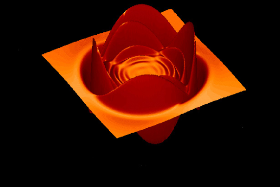
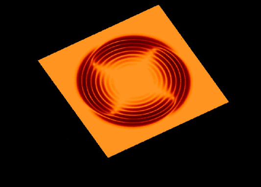
FIG. 2.: A spatial rendition of the quantity: ${i\sqrt{30}\over 8\sqrt{\pi}}\left(\psi_{(2,2)}e^{2i\phi}-\psi_{(2,-2)}e^{-2i\phi}\right)$. For large values of $r$ this is proportional to the “$\times$” strain of the gravitational wave that a detector would measure (see equation (24)). The proportionality factor is $100Mpc/r$. The overall vertical scaling is the same as in the figure of the quasi-normal ringing if $r=100Mpc$. In the attached movie one can see the time evolution leading to these pictures. The viewer should keep in mind that in order to visualize ”strain” a factor of $100Mpc/r$ should be included, and the strain is only a well defined concept in the far zone where the metric is approximately flat. The plot is for a given fixed colatitude $\theta=\pi/4$, as a function of $x,y$. The left picture is a side view, the right picture a top view. The picture corresponds to a snapshot at $t=80M$. The spatial scale is $\pm 100M$ in each direction. The vertical scale is the same as in figure 1.

In figure 2 we give a spatial visualization of the waves, by plotting the “$\times$” polarization of the waves, defined as,

$$h_{\times}={1\over r^{2}}h_{\theta\phi}={i\sqrt{30}\over 4r\sqrt{\pi}}\cos\theta\sin\theta\left(\psi_{(2,2)}e^{2i\phi}-\psi_{(2,-2)}e^{-2i\phi}\right),$$ (53)

The figure suggests a rotation pattern, but as can be seen in the accompanying movie, the shown patterns just propagate outward.

Let us turn now to the evaluation of the radiated energies and angular momentum. Figure 3 shows the radiated energy as a function of the initial angular momentum, for a fixed separation of the holes. The figure compares the Regge–Wheeler–Zerilli (Z) and Teukolsky (T) calculations. As expected, they differ for large values of the angular momentum, since the Teukolsky calculation contains terms higher than linear in the angular momentum. As we explained before, one is not keeping consistently these higher order terms so one cannot argue that the Teukolsky result is “better”. A conservative view that can be taken should be that both results disagree when higher order terms start to be important, and this gives us a rough measure of the error in the Zerilli calculation. We therefore conclude that for the separation in question, one should not trust first order perturbation theory beyond $a=0.5$. One should stress that this view can be somewhat overconservative, our experience with explicit second order calculations for the head-on collisions [36, 37, 30] shows that one should include all second order terms to have a consistent formulation and a reliable set of “error bars”. This is not accomplished by the first order Teukolsky formalism in this context. In this respect, second order Teukolsky results for this problem will be quite welcome [34]. The second order Zerilli calculations appear as quite prohibitive in complexity.

FIG. 3.: The radiated energy in a non-head-on collision of two non-spinning black holes as a function of the total initial angular momentum, for a fixed separation of $3.64$ radii (see text for details). We depict the results of treating the problem as a perturbation of a non-rotating hole (Z) and a rotating hole (T). The agreement of both curves up to angular momenta of $a=0.4-0.5$ gives confidence in the linear perturbative results. The “real data” very likely lies in a curve below the Zerilli (Z) curve, which allows us to roughly extrapolate the results to the extremal $a=1$ case, where we see that still less than $1\%$ of the mass of the system is radiated in the close limit.

The separation of the holes quoted in figure 3 requires some explanation. The simulations start with the construction of the initial data by the Bowen-York procedure we described in section II A. As discussed there, the construction starts with the introduction of a fiducial conformal space. In such a space the separation is $0.91M$ where $M$ is the ADM mass of the spacetime. The radius of each hole (if they were non-moving, the momentum slightly changes the shape of the horizon and the radius, see [25]) is approximately $M/4$, from there the separation of $3.64M$ quoted in the caption. To translate to more commonly used terms, one could convert the number to the $\mu_{0}$ parameter in the Misner solution, which for our case is $\mu_{0}=1.5$. Finally, another commonly used measure of the separation is the length of the geodesic threading the throat in the Misner geometry. In terms of such a parameter, it is equivalent to $2.75$ times the ADM mass of the spacetime or approximately $5.5$ times the mass of each individual hole.

A remarkable aspect of figure 3 is that linear perturbation theory has a tendency to overestimate the radiated energies for large values of the perturbative parameter, at least from our experience with head-on collisions of non-boosted [18], boosted [28] and some preliminary unpublished results we have for spinning holes. This would suggest that, if the same behavior takes place for the inspiralling collisions, “reality” should lie below the curve corresponding to the Regge–Wheeler–Zerilli formalism (Z). This would indicate that the estimation obtained using the Teukolsky formalism is actually worse for the particular kind of collision under consideration. This is what we were alluding to when we warned in the introduction that it was not obvious that representing the spacetime as a perturbation of a non-rotating hole was a worse choice than of that of a Kerr hole.

We now turn to the evaluation of the radiated angular momentum. This is depicted in figure 4.

FIG. 4.: Radiation of angular momentum. As can be seen, the Regge–Wheeler-Zerilli (Z) calculation of perturbations of a non-rotating hole disagrees with the Teukolsky (T) rotating black hole calculation. The radiated angular momentum is a more delicate quantity to compute than the energy and it appears that the potentially inconsistent higher order terms included in the rotating perturbation approach changes its value significantly. Overall we see the radiation is small. The Regge–Wheeler–Zerilli curve predicts less than $0.1\%$ of the total angular momentum will be radiated, even in the extreme rotating case.

The two curves shown in 4 disagree significantly. They do not even agree for very small values of the angular momentum. We have checked that there is no numerical error: if in the Teukolsky evolution one keeps the initial data intact but “turns off” the $a$-dependent terms in the evolution equation, the RWZ straight line is reproduced. It should be noticed that the radiated angular momentum is a qualitatively different quantity insofar as its computation than the energy. The energy is roughly obtained by squaring and integrating the waveforms. The angular momentum depends on subtle phase differences. It is much more easy to disturb the calculation of the radiated angular momentum than that of the radiated energy. This, in particular, points out to the potential difficulty of estimating this kind of quantity in full numerical simulations, where phase lags in the waveforms due to grid stretching and other problems are well known. In our approach it appears that the potentially inconsistent higher order terms in the angular momentum we introduce when considering a rotating background are causing problems in the computation of radiated angular momentum. If one wishes to be ultra-conservative, one could simply conclude that both calculations only predict the correct result for zero angular momentum. Otherwise, one could conclude that for this family of initial data the Teukolsky approach really only works for non-rotating black holes, something suggested by the fact that the background spacetime is only recovered in the close limit with vanishing angular momentum. At the moment we can only say that the accurate computation of the radiated angular momentum for this problem is an open problem. It is likely that the RWZ estimate is correct, but we do not have “error bars” (even rough ones) to validate this prediction.

VI Conclusions

We have used the “close limit” to estimate the radiation in the collision at the end of the inspiral of two equal mass nonrotating black holes. The assumptions and restrictions were: (i) only the “ringdown” radiation was computed; (ii) we assumed that a simple initial data set gave an adequate representation of appropriate astrophysical conditions; (iii) we assumed that the final hole is not near the extreme Kerr limit; (iv) we used close limit estimates of the evolution. Our main conclusion is that the energy radiated in ringdown is probably not more than 1% of the total mass of the system, and the angular momentum radiated is not more than 0.1% of the initial angular momentum. The most serious uncertainty in this result is the possibility that the radiation from the early merger stage of coalescence is very much larger than the ringdown radiation. With our 1%$Mc^{2}$ estimate, collisions of black holes of $100M_{\odot}$ would be detectable with signal to noise of 6 out to distances on the order of 200Mpc by the initial LIGO configuration and to distances of 4Gpc with the advanced LIGO detector.

VII Acknowledgements

We wish to thank two anonymous referees for many constructive criticisms on the initial submitted version of the paper. This work was supported in part by grants NSF-INT-9512894, NSF-PHY-9357219, NSF-PHY-9423950, NSF-PHY-9734871, NSF-PHY-9800973, NSF-PHY-9407194, by funds of the University of Córdoba, Utah, and Penn State. We also acknowledge support of CONICET and CONICOR (Argentina). JP acknowledges support from the the John S. Guggenheim foundation and hospitality from ITP at UC Santa Barbara during completion of the manuscript. RJG is a member of CONICET.

REFERENCES

- [1] See for instance, E. Seidel, in “Gravitation and relativity: At the turn of the millennium”, N. Dahdhich, J. Narlikar (eds.), Inter University Center for Astronomy and Astrophysics, Poona, India (1998).
- [2] K. Schwarzschild, Sitz. Preuss. Akad. Wiss. 189 (1916).
- [3] See P. Anninos, D. Hobill, E. Seidel, L. Smarr and W. Suen, Phys. Rev. D52, 2044 (1995) and references therein.
- [4] For current information and links to all the interferometric gravitational wave detector projects see http://www.ligo.caltech.edu.
- [5] For a recent discussion see S. Zwart, S. MacMillan, astro-ph/9910061, to appear in Ap. J. Lett.
- [6] For a review on sources of gravitational waves see K. Thorne, gr-qc/9704042.
- [7] For a review on post-Newtonian approximations see C. Will, gr-qc/9910057, to appear in Prog. Theor. Phys.
- [8] A. Ptak, R. Griffiths, Astroph. J. 517, L85 (1999); E. Colbert, R. Mushotzky, Astroph. J. 519, 89 (1999).
- [9] http://lisa.jpl.nasa.gov, http://www.lisa.uni-hannover.de/
- [10] T. Regge and J. Wheeler, Phys. Rev. 108, 1063 (1957).
- [11] F. J. Zerilli, Phys. Rev. Lett. 24 737 (1970).
- [12] S. Teukolsky, Ap. J. 185, 635 1973).
- [13] M. Davis, R. Ruffini, W. Press, R. Price, Phys. Rev. Lett. 27, 1466 (1971).
- [14] See the discussion in E. Flanagan, S. Hughes, Phys. Rev. D57, 4535 (1997).
- [15] For a recent review see J. Pullin, Prog. Theor. Phys. (in press), gr-qc/9909021.
- [16] For a good discussion see the article by J. York in “Sources of gravitational radiation”, L. Smarr (ed.), Cambridge ????.
- [17] C. Misner, Phys. Rev. 118, 1110 (1960).
- [18] R. Price, J. Pullin, Phys. Rev. Lett. 72, 3638 (1994).
- [19] P. Anninos, R. Price, J. Pullin, E. Seidel, W.-M. Suen, Phys. Rev. D52, 4462 (1995).
- [20] A. Abrahams, G. Cook, Phys. Rev. D50, 2364 (1994), see also J. Baker, C. B. Li, Class. Quant.Grav. 14 L77 (1997).
- [21] R. Gleiser, C. Nicasio, R. Price, J. Pullin, Class. Quan. Grav. 13, L117-L124 (1996); Phys. Rev. Lett 77, 4483 (1996); Phys. Rev. D59, 044024 (1999); ref [30].
- [22] J. Bowen, J. York, Phys. Rev. D21, 2047 (1980).
- [23] B. Brügmann, S. Brandt, Phys. Rev. Lett. 78, 3606-3609 (1997) .
- [24] R. Gleiser, O. Nicasio, R. Price, J. Pullin, Phys. Rev. 57, 3401 (1998).
- [25] G. Cook, J. York, Phys. Rev. D41, 1077 (1990).
- [26] D. Brill, R. Lindquist, Phys. Rev. 131, 471 (1963).
- [27] A.M. Abrahams and R.H. Price, Phys. Rev. D53, 1972 (1996).
- [28] J. Baker, A. Abrahams, P. Anninos, S. Brandt, R. Price, J. Pullin and E. Seidel, Phys. Rev. D55, 829 (1997)
- [29] F. J. Zerilli, Phys. Rev. D2 2141 (1970).
- [30] R. Gleiser, C. Nicasio, R. Price, J. Pullin, Phys. Rep. (in press) gr-qc/9807077.
- [31] C. T. Cunningham, R. H. Price and V. Moncrief, Astrophys. J. 224, 643 (1978); 230, 870 (1979); 236, 674 (1980); in Sources of Gravitational Radiation, ed. L. Smarr (Cambridge University Press, 1979).
- [32] K.S. Thorne, Rev. Mod. Phys. 52, 299 (1980).
- [33] M. Campanelli, C.O. Lousto, J. Baker, G. Khanna and J. Pullin, Phys. Rev. D58, 084019 (1998)
- [34] M. Campanelli, C. Lousto, Phys. Rev. D59, 124022 (1999).
- [35] W. Krivan, P. Laguna, P. Papadopoulos and N. Andersson, Phys. Rev. D56, 3395 (1997).
- [36] R. Gleiser, O. Nicasio, R. Price, J. Pullin, Phys. Rev. Lett. 77, 4483 (1996).
- [37] C.O. Nicasio, R.J. Gleiser, R.H. Price and J. Pullin, Phys. Rev. D59, 044024 (1999).