Padé approximants for truncated post-Newtonian neutron star models

Abstract

Padé approximants to truncated post-Newtonian neutron star models are constructed. The Padé models converge faster to the general relativistic (GR) solution than the truncated post-Newtonian ones. The evolution of initial data using the Padé models approximates better the evolution of full GR initial data than the truncated Taylor models. In the absence of full GR initial data (e.g., for neutron star binaries or black hole binary systems), Padé initial data could be a better option than the straightforward truncated post-Newtonian (Taylor) initial data.

I Introduction

Compact binary systems of neutron stars and black holes inspiralling under gravitational radiation reaction are one of the most promising sources of gravitational waves for kilometre arm length interferometric gravitational wave detectors like the LIGO and VIRGO. The inspiral phase is best described by a post-Newtonian approximation which should eventually break down and the final merger and coalescence may be only accessible via numerical integration of Einstein’s equations. A major obstacle in the numerical studies of such systems is the non-availability of physically satisfactory initial data. Given the constraints on computational resources, one would like to start the numerical integration as close as possible to the final coalescence phase, using the initial data obtained by matching on to the known analytical results of inspiral. One of the suggestions in this direction is to use the analytical post-Newtonian results of inspiral to provide initial data (e.g. [1]-[2]) for the numerical integration of the fully general relativistic system.

Before attempting to apply the above strategy to the complicated compact binary system, as a preliminary step, Shinkai [3] has constructed a single neutron star model using the post-Newtonian approach and concluded that the truncated second order post-Newtonian approximation is close enough to describe a general relativistic single star. The truncated post-Newtonian series used above is essentially a Taylor expansion in the three small parameters $A=p/(\rho_{t}c^{2})$, $B=4\pi pr^{3}/(mc^{2})$ and $C=2Gm/(rc^{2})$ where $p$ is the pressure, $\rho_{t}$, the total energy density of the system, $r$ the radial coordinate, and $m(r)$ the mass contained in a sphere of radial coordinate $r$. We shall refer to the post-Newtonian truncated models alternatively as Taylor models. Recently, in a related context of gravitational wave phasing, the slow convergence of straightforward Taylor approximants has been critically investigated[4][5]. It was shown that new approximants, with much improved convergence properties, may be constructed for gravitational wave data analysis applications using, as an important tool, Padé techniques to estimate the relevant functions from only the first few terms in their perturbative post-Newtonian expansion. This approach has been systematically extended in a series of publications [6][7] and most recently has been used to go beyond the adiabatic approximation to inspiral and provide an analysis of the transition from the inspiral to the plunge in binary black hole coalescences [2]. This work also provides for the first time initial dynamical data (positions and momenta) for binary black holes starting to plunge, so that there is less than an orbit left to evolve. In view of this experience, in this report, we construct Padé approximants to the truncated post-Newtonian (Taylor) neutron star models discussed by Shinkai [3] and investigate their performance. We show that the Padé models are better than the truncated post-Newtonian models and converge faster to the exact general relativistic solution. Further, we also show that the evolution of a general relativistic (single) star is described much better by Padé initial data as compared to the truncated Taylor initial data of the same order.

In the next section we discuss the TOV equation and the truncated post-Newtonian models. In Section III we introduce the standard Padé approximant, discuss its applicability to the present problem, and adapt it to construct an appropriate generalisation for the case of 3-small parameters. Padé models corresponding to the ‘Taylor’ truncated models are constructed. In the last section we discuss the results and summarise our conclusions. The Appendix lists the more involved formulas for the 3PN Padé models.

II TOV equation and truncated post-Newtonian (Taylor) neutron star models

In general relativity the metric of a spherically symmetric static star can be written as

$$ds^{2}=-e^{2\nu(r)}dt^{2}+e^{2\lambda(r)}dr^{2}+r^{2}(d\theta^{2}+r^{2}\sin^{2}\theta d\phi^{2}),$$ (1)

and the equations of hydrostatic equilibrium - the Tolman-Oppenheimer-Volkoff (TOV) equations - obtained (in geometrised units: $G=c=M_{\odot}=1$) from the Einstein field equations, for a given fluid distribution specified by an adiabatic equation of state $p=p(\rho_{t})$, are given by:

$$\frac{dm}{dr} = 4\pi r^{2}\rho_{t},$$ (2)

$$\frac{dp}{dr} = -\frac{m\rho_{t}}{r^{2}}\left(1+\frac{p}{\rho_{t}}\right)\left(1+\frac{4\pi pr^{3}}{m}\right)\left(1-\frac{2m}{r}\right)^{-1},$$ (3)

$$\frac{d\nu}{dr} = \frac{m}{r^{2}}\left(1+\frac{4\pi pr^{3}}{m}\right)\left(1-\frac{2m}{r}\right)^{-1}.$$ (4)

$m$ is given in terms of metric component $\lambda$ as

$$e^{2\lambda}=\left(1-\frac{2m}{r}\right)^{-1}.$$ (5)

The above set of equations are integrated from the center ($r=0$) to the boundary of the star, with the initial conditions $m(r=0)=0;\rho_{t}(r=0)=\rho_{t_{c}}$ and $\nu{(r=0)}=\nu_{c}$. $\nu_{c}$ is rescaled appropriately such that it matches with the exterior Schwarzschild solution at the boundary. The radius of the star, $R$, is characterised as the radius where density $\rho_{t}(r=R)$ drops to $10^{6}$ gm/cc (approximately ${\cal O}(10^{-10})$ in geometrised units).

Schematically, equations (3) and (4) can be written as

$$\frac{dp}{dr} = -\frac{m\rho_{t}}{r^{2}}(1+A)(1+B)(1-C)^{-1}\,,$$ (6)

$$\frac{d\nu}{dr} = \frac{m}{r^{2}}(1+B)(1-C)^{-1}.$$ (7)

Assuming that $A$, $B$ and $C$ are of comparable orders of smallness and making a Taylor series expansion in $A$, $B$, and $C$ around the origin, the above equations to third post-Newtonian order then yield,

$$\frac{dp}{dr} = -\frac{m\rho_{t}}{r^{2}}(1+\underbrace{A+B+C}_{1PN}+\underbrace{AB+BC+CA+C^{2}}_{2PN}$$ (9)

$$+\underbrace{ABC+AC^{2}+BC^{2}+C^{3}}_{3PN}+{\cal O}(4)\cdots)\,,$$

$$\frac{d\nu}{dr} = \frac{m}{r^{2}}(1+\underbrace{B+C}_{1PN}+\underbrace{BC+C^{2}}_{2PN}+\underbrace{BC^{2}+C^{3}}_{3PN}+{\cal O}(4)\cdots)\,,$$ (10)

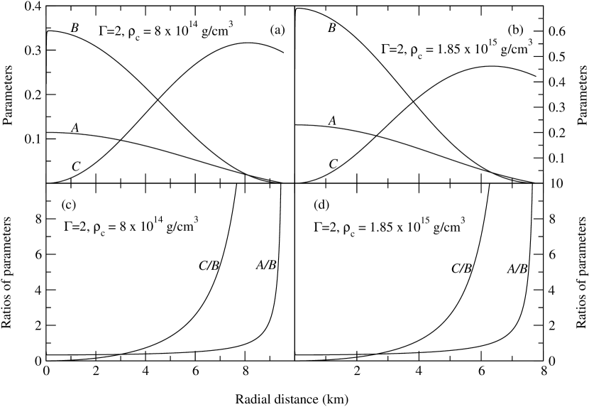
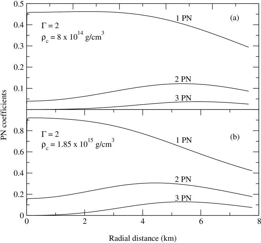
where the post-Newtonian order of the relevant terms is indicated by the PN label under the braces. These equations describe the truncated post-Newtonian model [3]. Before proceeding ahead, we must verify that the above truncation is consistent and meaningful in the present problem of neutron stars. For a range of models, we evaluate the successive combinations that appear in Eqs. (9) and (10), using the exact TOV equations. Figure 1 shows the combinations appearing in Eq. (9) for two such models with an equation of state of intermediate stiffness, one which is very close to the maximum mass limit and another, a little further down the stable branch. From the Figure it is clear that numerically the successive combinations are perturbatively smaller to be consistently denoted as 1PN, 2PN and 3PN contributions.

III Padé approximants to the truncated post-Newtonian (Taylor) models

Given a Taylor series of order $n$ in one expansion parameter $x$

$$S_{n}(x)=1+a_{1}x+\cdots+a_{n}x^{n},$$ (11)

its Padé approximant is the ratio of rational functions,

$$P^{m}_{k}(x)=\frac{N_{m}(x)}{D_{k}(x)},$$ (12)

satisfying the condition

$$T_{n}[P^{m}_{k}(x)]\equiv S_{n}(x);\;\;\;\;k+m=n.$$ (13)

In the above, $N_{m}$ and $D_{k}$ are polynomials in $x$ of order $m$ and $k$ respectively and $T_{n}$ denotes the operation of expanding a function in Taylor series upto order $n$.

A convenient choice of Padé approximants is its diagonal (or nearly diagonal) continued fraction form [8] i.e., $P^{m}_{m}$ when $n=2m$ (even) and $P^{m}_{m+1}$ when $n=2m+1$ (odd). For instance,

$$P^{1}_{2}=\frac{c_{0}}{1+\displaystyle{\frac{c_{1}x}{1+\displaystyle{\frac{c_{2}x}{1+c_{3}x}}}}}\,,$$ (14)

where the $c_{i}$’s are determined in terms of the Taylor coefficients $a_{i}$ by

$$c_{0}=1,\;\;c_{1}=-a_{1},\;\;c_{2}=\frac{a_{1}^{2}-a_{2}}{a_{1}},\;\;c_{3}=\frac{a_{1}a_{3}-a_{2}^{2}}{a_{1}(a_{1}^{2}-a_{2})}\,.$$ (15)

To construct the Padé approximant of the truncated post-Newtonian models discussed in the previous section, we must proceed carefully. In the problem under discussion, in general, there are three independent small parameters $A$, $B$, $C$, of the same order of smallness. Given this system of approximate differential equations containing three independent small parameters, can we construct an associated Padé like approximation with faster and improved convergence? Assume for a moment, that since $A$, $B$, $C$ are of the same order of smallness, we decide to use as the variable of expansion the parameter $B$ that takes the maximum value in the entire range of integration. The first order Taylor term $A+B+C$ would be rewritten as $B(1+A/B+C/B)$. If we treat only $B$ as the independent variable then its associated coefficient would be $1+A/B+C/B$. If $A/B$ and $C/B$ have only a weak dependence on $r$, we can indeed use a simpler Padé form with only one variable and this should suffice. We call this the one parameter Padé form for the TOV equations. In this case, the relevant equations at 2PN are the following:

$$\frac{dm}{dr} = 4\pi r^{2}\rho_{t}\,,$$ (17)

$$\frac{dp}{dr} = -\frac{m\rho_{t}}{r^{2}}\frac{1}{{\cal F}_{2}}\,,$$ (18)

$$\frac{d\nu}{dr} = \frac{m}{r^{2}}\frac{1}{{\cal G}_{2}}\,,$$ (19)

$${\rm where},\;\;{\cal F}_{2} = \frac{A+B+C-AB-BC-CA-C^{2}}{A+B+C+A^{2}+AB+CA+B^{2}+BC}\,,$$ (20)

$${\rm and},\;\;{\cal G}_{2} = \frac{B+C-BC-C^{2}}{B+C+B^{2}+BC}\,.$$ (21)

(The more involved equations at 3PN are listed in the Appendix). To examine more quantitatively, the validity of the above treatment, we consider, as before, a few models and compute the values of $A$, $B$ and $C$ and the associated ratios of $A/B$ and $C/B$. The results are displayed in Figure 2. From the figure it is clear, that as required, $A$, $B$, $C$ are approximately of the same order of smallness. However, if one looks at the ratio of $C/B$, one finds that there is a regime where the $r$-dependence is not very weak. Consequently, we are wary of using only the usual straightforward one parameter Padé form discussed above and proceed as follows. We generalise the usual construction for the one parameter Padé to the situation where there exist, not one, but three small parameters. The advantage of using a three parameter form is that its ‘coefficients’ are pure numbers with no explicit ‘$r$-dependence’. By treating $A$, $B$, $C$ as independent variables, we avoid the explicit issue of the ‘weak $r$-dependence’ of the associated coefficients.

To this end, we start with the most general second order post-Newtonian accurate polynomial in three small parameters $A$, $B$ and $C$ as

$$T_{2} = 1+t_{A}A+t_{B}B+t_{C}C+t_{AA}A^{2}+t_{BB}B^{2}+t_{CC}C^{2}$$ (23)

$$+t_{AB}AB+t_{BC}BC+t_{CA}CA\,.$$

The associated Padé approximant in continued fraction form may be chosen as

$$P^{1}_{1}=\frac{1}{F_{2}}\,,$$ (24)

where

$$F_{2} = 1+\frac{p_{1}A}{1+p_{11}A+p_{12}B+p_{13}C}+$$ (26)

$$\frac{p_{2}B}{1+p_{21}A+p_{22}B+p_{23}C}+\frac{p_{3}C}{1+p_{31}A+p_{32}B+p_{33}C}\,.$$

By matching coefficients of the Taylor expansion of $P^{1}_{1}$, Eq. (24), and $T_{2}$, Eq. (23), the three coefficients $p_{1}$, $p_{2}$ and $p_{3}$ are uniquely determined as,

$$p_{1}=-t_{A};\;\;\;p_{2}=-t_{B};\;\;\;p_{3}=-t_{C}.$$ (27)

The remaining nine coefficients $p_{ij}$, where $i,j=1,2,3$, are not uniquely determined; they are solutions to the following (under-determined) system of six equations

$$t_{A}(t_{A}-p_{11}) = t_{AA}\,,$$ (29)

$$t_{B}(t_{B}-p_{22}) = t_{BB}\,,$$ (30)

$$t_{C}(t_{C}-p_{33}) = t_{CC}\,,$$ (31)

$$t_{A}p_{12}+t_{B}p_{21} = 2t_{A}t_{B}-t_{AB}\,,$$ (32)

$$t_{B}p_{23}+t_{C}p_{32} = 2t_{B}t_{C}-t_{BC}\,,$$ (33)

$$t_{C}p_{31}+t_{A}p_{13} = 2t_{C}t_{A}-t_{CA}\,.$$ (34)

If $t_{A}\neq 0$, $t_{B}\neq 0$, $t_{C}\neq 0$, $p_{11}$, $p_{22}$ and $p_{33}$, can also be uniquely determined using Eqs. (29), (30) and (31) respectively. We have

$$p_{11} = \frac{t_{A}^{2}-t_{AA}}{t_{A}},$$ (36)

$$p_{22} = \frac{t_{B}^{2}-t_{BB}}{t_{B}},$$ (37)

$$p_{33} = \frac{t_{C}^{2}-t_{CC}}{t_{C}}.$$ (38)

The remaining six non-diagonal terms cannot be uniquely determined from the remaining three equations Eq. (32) - (34) without further input. The natural requirement that all Padé coefficients $p_{ij}$ contributing to a particular Taylor term, contribute equally, leads one to the following symmetry choice

$$p_{12}=p_{21},\;\;p_{23}=p_{32},\;\;p_{13}=p_{31}.$$ (39)

One can then uniquely determine all the required coefficients and finally obtain

$$p_{12}=p_{21} = \frac{2t_{A}t_{B}-t_{AB}}{t_{A}+t_{B}},\;\;{\rm if}\;\;\;t_{A}+t_{B}\neq 0,$$ (41)

$$p_{23}=p_{32} = \frac{2t_{B}t_{C}-t_{BC}}{t_{B}+t_{C}},\;\;{\rm if}\;\;\;t_{B}+t_{C}\neq 0,$$ (42)

$$p_{31}=p_{13} = \frac{2t_{C}t_{A}-t_{CA}}{t_{C}+t_{A}},\;\;{\rm if}\;\;\;t_{C}+t_{A}\neq 0.$$ (43)

Since the form of Eq. (9) is equivalent to Eq. (23) and Eq. (7) has a less general form containing only 2-parameters $B$ and $C$, the second order Padé approximant to the second order truncated TOV equations may be written as

$$\frac{dm}{dr} = 4\pi r^{2}\rho_{t}\,,$$ (44)

$$\frac{dp}{dr} = -\frac{m\rho_{t}}{r^{2}}\frac{1}{F_{2}}\,,$$ (45)

$$\frac{d\nu}{dr} = \frac{m}{r^{2}}\frac{1}{G_{2}}\,,$$ (46)

where $F_{2}$ is given by Eq. (26) and $G_{2}$ is obtained by substituting $A=0$ in $F_{2}$ . A comparison of Eqs. (9) and (23) yields

$$t_{A}=t_{B}=t_{C}=t_{AB}=t_{BC}=t_{CA}=t_{CC}=1,$$ (48)

$$t_{BB}=t_{AA}=0,$$ (49)

so that the $p_{ij}$ (Eqs. (36)-(38) and (41)-(43)) in this case become

$$p_{11}=p_{22}=1,\;\;p_{33}=0\,,$$ (51)

$$p_{12}=p_{23}=p_{13}=\frac{1}{2}\,.$$ (52)

The associated forms of $F_{2}$ and $G_{2}$ are finally given by

$$F_{2} = 1-\frac{A}{1+A+\frac{B+C}{2}}-\frac{B}{1+B+\frac{A+C}{2}}-\frac{C}{1+\frac{A+B}{2}}\;,$$ (53)

$$G_{2} = 1-\frac{B}{1+B+\frac{C}{2}}-\frac{C}{1+\frac{B}{2}}\;.$$ (54)

Equations (53) and (54) define the three parameter 2PN Padé model associated with the 2PN truncated model discussed in [3]. The 3PN three parameter Padé model may be similarly obtained but since the expressions are lengthier, we list them in the Appendix together with the one parameter 3PN Padé model.

IV Results and Discussion

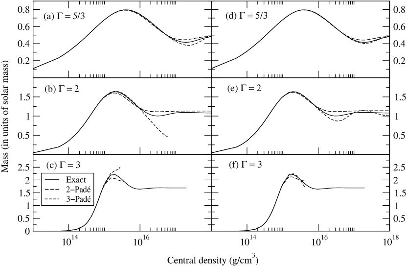
We consider the polytropic equation of state $p=K\rho^{\Gamma}$ choosing the same models as studied by Shinkai [3] i.e., $\Gamma=5/3,2$ and $3$ with $K$ (the polytropic constant) $=4.35,10^{2}$ and $10^{5}$, respectively. Before presenting the final results, we have compared the performance of the one parameter Padé models with three parameter Padé models and display in Figure 3 a typical comparison. From the Figure it is clear that both models yield similar numerical performance and the difference, if any, appears in the region where anyway these models are not recommended. Consequently, all our Figures refer to the one parameter Padé models though we have verified that the three parameter Padé models also yield similar results.

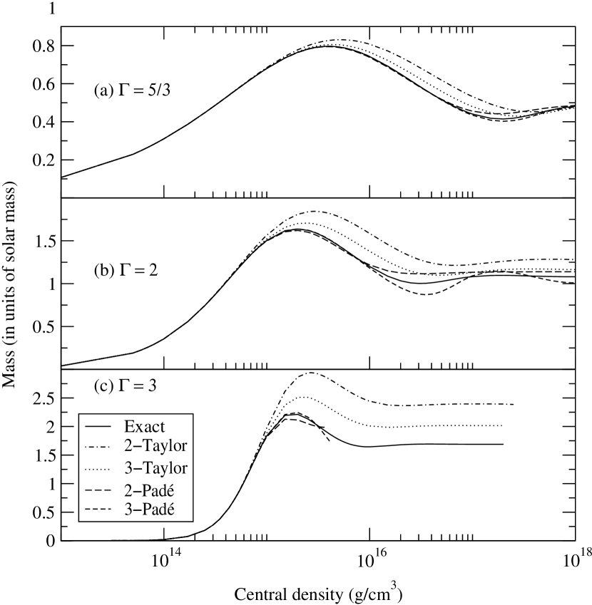
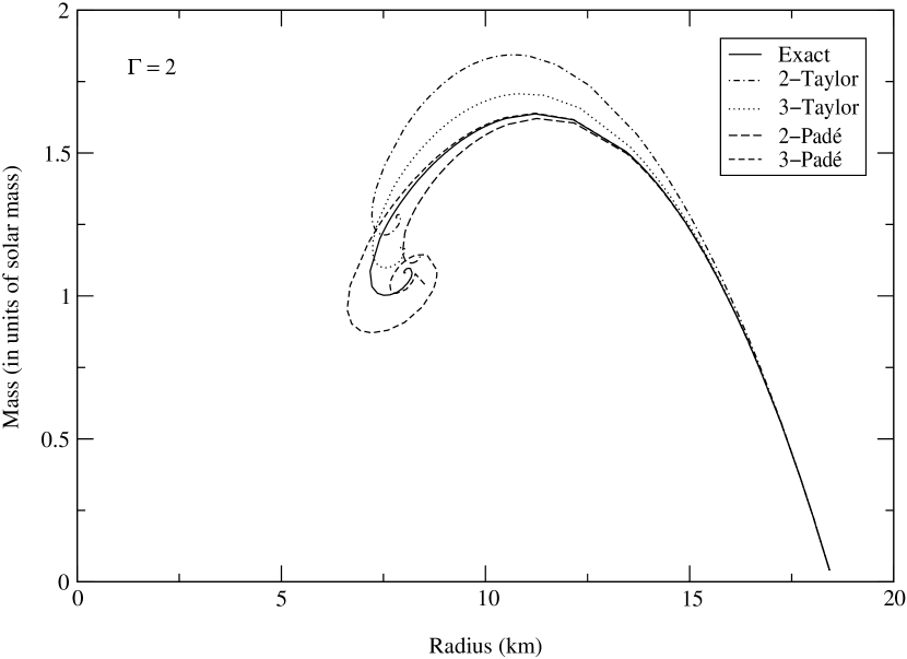
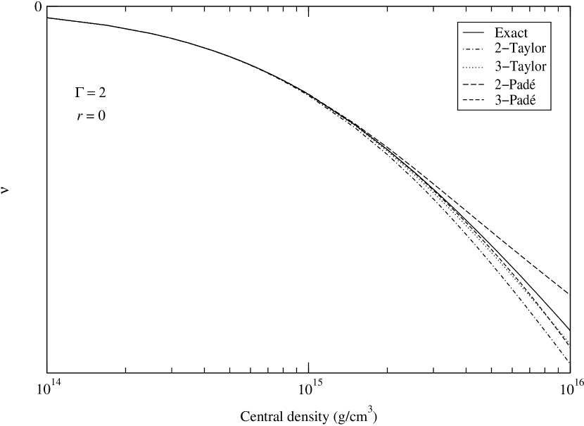
In Fig. 4, we plot mass (in solar mass units) as a function of central density. The different curves represent the exact TOV, the 2PN and 3PN truncated (Taylor) models (henceforth 2-Taylor, 3-Taylor etc; for more details, see [3]) and our new Padé approximated models. We do not plot curves corresponding to 1PN truncated Taylor and the associated first order Padé model as they are very far away from the exact GR curve and thus evidently inadequate. It is very clear from the figure that for all models to the left of the (first) maximum, which represents the stable branch of the mass-density curve, the Padé models do extremely well as compared to Taylor models. In this regime the third order Padé (now onwards 3-Padé) curve (dashed line) is very close to the exact GR curve (solid line). The 2-Padé (long-dashed line) curve is not only better compared to the 2-Taylor one (dot-dashed) but even far better than the 3-Taylor curve (dotted line). In the unstable branch i.e., to the right to the maximum, the Padé approximation starts becoming bad. This feature is more severe when the stiffness of the considered equation of state and the order of the Padé approximants are higher (Fig. 4b and c). However, the stable branch is approximated well by Padé models even for a very stiff equation of state ($\Gamma=3$, Fig. 4c), where the approximation breaks down near ($2.75$ x $10^{15}$ g/cm³) the maximum mass limit ($1.85$ x $10^{15}$ g/cm³). Studies of mass-radius curves and $\nu_{c}$ (the exponent of the metric component $g_{tt}$ at the center of the star) vs central density curves also show a similar dependence on the stiffness of the chosen equation of state and on the central density. In Fig. 5 and Fig. 6, we plot mass vs radius and $\nu_{c}$ vs central density curves respectively, for an equation of state with intermediate stiffness $\Gamma=2$. The deviation of the 3-Padé solutions from the exact GR ones correspond to the configurations lying on the unstable branch.

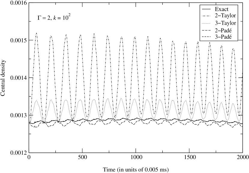
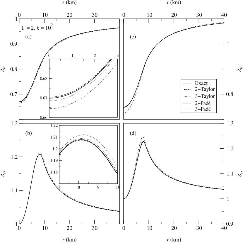
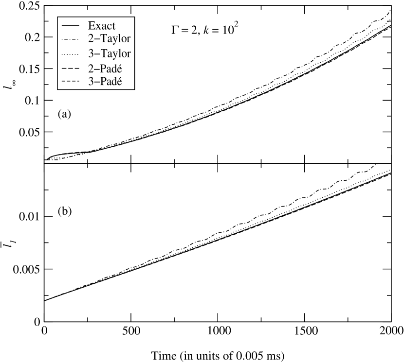
The studies of these equilibrium configurations imply clearly that the stable general relativistic TOV configurations are approximated very well by Padé models as compared to Taylor truncated models, even if they do not perform so well in the unstable branch. To study this further, we next numerically evolve these five initial configurations - Exact TOV, 2-Padé, 3-Padé, 2-Taylor and 3-Taylor truncated models - in time and qualitatively compare their evolution. We use a spherically symmetric general relativistic hydrodynamical code for this purpose [9]. The code uses polar slicing and radial gauge. The spacetime is evolved using the ADM formalism and the hydrodynamic evolution is based on a high resolution shock capturing [10]-[11] scheme. The grid boundary is fixed at about four times the radius of the TOV model. We choose a model with central density $1.28$ x $10^{-3}$ (geometrised units), $\Gamma=2,k=10^{2}$ and then evolve it upto 10 ms (though the code runs for a much longer time, 10 ms evolution is sufficient for our analysis). In Fig. 7 the evolution of central density using various initial data is displayed. We find that the 3-Padé curve follows the TOV evolution curve very closely. Even the 2-Padé evolution is much better than the 3-Taylor and the 2-Taylor evolutions. The oscillations in the central density are due to the numerical truncation errors which introduce non-zero radial velocity. These truncation errors act as the small perturbations on a stable spherically symmetric configuration and give rise to the radial pulsation modes of the system. A Fourier transform of the density or radial velocity evolution can be used to extract these pulsation modes [12] and we hope to return to this in a subsequent work. In Fig. 8 we plot the metric components $g_{tt}$ and $g_{rr}$ over the grid for $t=0$ (initial time) and $t=10$ ms (final time). To compare the global performance of the initial data used (the exact TOV and the various truncated models), the norms of the Hamiltonian constraints $l_{\infty}$ (maximum value at a given time step) and ${\bar{l}}_{1}$ (average of the absolute value) are evaluated and shown in Fig. 9. These figures, once again, confirm the superior performance of Padé approximants over Taylor approximants of the same order. Though we do not display them, we get similar results for the other stable configurations both for relatively softer and stiffer equations of state. A final comment on the models in the unstable branch of the mass-density curve: the truncation errors are enough to trigger a collapse and make the system unstable on a time scale so short that a comparison of various approximations is not possible. A more detailed analysis would be needed in this regard.

To conclude: Detailed studies of equilibrium configurations of single neutron stars and their evolution indicate, that in the stable branch, the second order Padé model converges to the exact general relativistic model even better than the straightforward third order truncated (Taylor) PN model. Both the simpler one parameter Padé form and a more involved three parameter Padé form exhibit similar improvement over the Taylor models. The Padé models are thus quite robust and controlled and perform better than the simpler Taylor truncated models. It is better to use initial data obtained from a Padé approximant to the Taylor model than initial data from a straightforward post-Newtonian truncated model of the same order. This feature should be generic and extend to binary neutron stars and black holes [especially since a useful simplification in a two-body problem is via a reduction to an equivalent one-body problem] and prove useful in numerical studies of such systems in the future.

A

The 3PN truncated model in general has the form

$$T_{3} = 1+t_{A}A+t_{B}B+t_{C}C+$$ (A4)

$$t_{AA}A^{2}+t_{BB}B^{2}+t_{CC}C^{2}+t_{AB}AB+t_{BC}BC+t_{CA}CA+$$

$$t_{AAA}A^{3}+t_{BBB}B^{3}+t_{CCC}C^{3}+t_{ABC}ABC+$$

$$t_{AAB}A^{2}B+t_{BBC}B^{2}C+t_{CCA}C^{2}A+t_{ABB}AB^{2}+t_{BCC}BC^{2}+t_{AAC}A^{2}C\,.$$

The associated 3PN Padé may be written as

$$P_{3} = \frac{1}{F_{3}},$$ (A6)

$${\rm where}\;F_{3} = 1+\frac{p_{1}A}{1+\frac{p_{11}A}{S_{11}}+\frac{p_{12}B}{S_{12}}+\frac{p_{13}C}{S_{13}}}+$$ (A8)

$$\frac{p_{2}B}{1+\frac{p_{21}A}{S_{21}}+\frac{p_{22}B}{S_{22}}+\frac{p_{23}C}{S_{23}}}+\frac{p_{3}C}{1+\frac{p_{31}A}{S_{31}}+\frac{p_{32}B}{S_{32}}+\frac{p_{33}C}{S_{33}}}\,,$$

where $S_{ij}=1+p_{ij1}A+p_{ij2}B+p_{ij3}C$, $i,j=1\ldots 3$. The analysis discussed in Sec. III at 2PN may be repeated at 3PN after making the following natural symmetric choice implied by the requirement that all Padé coefficients contributing to a particular Taylor term contribute equally:

$$p_{112} = p_{121}=p_{211}\,,$$ (A10)

$$p_{122} = p_{221}=p_{212}\,,$$ (A11)

$$p_{113} = p_{131}=p_{311}\,,$$ (A12)

$$p_{123} = p_{132}=p_{231}=p_{213}=p_{312}=p_{321}\,,$$ (A13)

$$p_{313} = p_{331}=p_{133}\,,$$ (A14)

$$p_{322} = p_{232}=p_{223}\,,$$ (A15)

$$p_{332} = p_{233}=p_{323}\,.$$ (A16)

The remaining $10$ independent $3$PN Padé coefficients, uniquely determined by 1PN, 2PN and 3PN Taylor coefficients, are given by

$${\it p_{111}} = {\frac{-{t_{{{\it AA}}}}^{2}+t_{{{\it AAA}}}t_{{A}}}{t_{{A}}\left({t_{{A}}}^{2}-t_{{{\it AA}}}\right)}}\,,$$ (A18)

$${\it p_{222}} = {\frac{-{t_{{{\it BB}}}}^{2}+t_{{{\it BBB}}}t_{{B}}}{t_{{B}}\left({t_{{B}}}^{2}-t_{{{\it BB}}}\right)}}\,,$$ (A19)

$${\it p_{333}} = {\frac{-{t_{{{\it CC}}}}^{2}+t_{{{\it CCC}}}t_{{C}}}{t_{{C}}\left({t_{{C}}}^{2}-t_{{{\it CC}}}\right)}}\,,$$ (A20)

$${\it p_{112}} = \biggl{\{}\biggl{[}-{t_{{A}}}^{4}t_{{B}}+2\,{t_{{B}}}^{2}{t_{{A}}}^{3}+\left(-{t_{{B}}}^{3}+\left(-2\,t_{{{\it AB}}}+2\,t_{{{\it AA}}}\right)t_{{B}}+t_{{{\it AAB}}}\right){t_{{A}}}^{2}$$ (A24)

$$+\left(-2\,t_{{{\it AA}}}t_{{{\it AB}}}+2\,t_{{{\it AAB}}}t_{{B}}+2\,{t_{{B}}}^{2}t_{{{\it AB}}}\right)t_{{A}}-2\,t_{{{\it AA}}}{t_{{B}}}^{3}+t_{{{\it AAB}}}{t_{{B}}}^{2}$$

$$-t_{{{\it AB}}}\left(2\,t_{{{\it AA}}}+t_{{{\it AB}}}\right)t_{{B}}\biggr{]}\biggr{\}}$$

$$\biggl{\{}\left(t_{{B}}+t_{{A}}\right)^{2}\left(2\,t_{{A}}t_{{B}}-t_{{{\it AA}}}-t_{{{\it AB}}}+{t_{{A}}}^{2}\right)\biggr{\}}^{-1}\,,$$

$${\it p_{122}} = \biggl{\{}\biggl{[}\left(-{t_{{B}}}^{2}-2\,t_{{{\it BB}}}\right){t_{{A}}}^{3}+\left(2\,t_{{B}}t_{{{\it AB}}}+2\,{t_{{B}}}^{3}+t_{{{\it ABB}}}\right){t_{{A}}}^{2}$$ (A28)

$$+\left(-{t_{{B}}}^{4}+\left(2\,t_{{{\it BB}}}-2\,t_{{{\it AB}}}\right){t_{{B}}}^{2}+2\,t_{{{\it ABB}}}t_{{B}}-t_{{{\it AB}}}\left(t_{{{\it AB}}}+2\,t_{{{\it BB}}}\right)\right)t_{{A}}$$

$$-2\,t_{{{\it AB}}}t_{{{\it BB}}}t_{{B}}+t_{{{\it ABB}}}{t_{{B}}}^{2}\biggr{]}\biggr{\}}$$

$$\biggl{\{}\left(t_{{B}}+t_{{A}}\right)^{2}\left({t_{{B}}}^{2}+2\,t_{{A}}t_{{B}}-t_{{{\it AB}}}-t_{{{\it BB}}}\right)\biggr{\}}^{-1}\,,$$

$${\it p_{113}} = \biggl{\{}\biggl{[}-t_{{C}}{t_{{A}}}^{4}+2\,{t_{{A}}}^{3}{t_{{C}}}^{2}+\left(-{t_{{C}}}^{3}+\left(2\,t_{{{\it AA}}}-2\,t_{{{\it AC}}}\right)t_{{C}}+t_{{{\it AAC}}}\right){t_{{A}}}^{2}$$ (A32)

$$+\left(-2\,t_{{{\it AA}}}t_{{{\it AC}}}+2\,{t_{{C}}}^{2}t_{{{\it AC}}}+2\,t_{{{\it AAC}}}t_{{C}}\right)t_{{A}}-2\,t_{{{\it AA}}}{t_{{C}}}^{3}+t_{{{\it AAC}}}{t_{{C}}}^{2}$$

$$-t_{{{\it AC}}}\left(t_{{{\it AC}}}+2\,t_{{{\it AA}}}\right)t_{{C}}\biggr{]}\biggr{\}}$$

$$\biggl{\{}\left(t_{{A}}+t_{{C}}\right)^{2}\left({t_{{A}}}^{2}+2\,t_{{C}}t_{{A}}-t_{{{\it AA}}}-t_{{{\it AC}}}\right)\biggr{\}}^{-1}\,,$$

$${\it p_{123}} = \biggl{\{}\biggl{[}\left(-2\,{t_{{B}}}^{2}t_{{C}}+\left(-2\,{t_{{C}}}^{2}-2\,t_{{{\it BC}}}\right)t_{{B}}-2\,t_{{{\it BC}}}t_{{C}}\right){t_{{A}}}^{3}$$ (A42)

$$+\biggl{(}-2\,t_{{C}}{t_{{B}}}^{3}+\left(2\,t_{{{\it BC}}}+2\,t_{{{\it AC}}}+12\,{t_{{C}}}^{2}\right){t_{{B}}}^{2}$$

$$+\left(-2\,{t_{{C}}}^{3}+\left(2\,t_{{{\it AB}}}-4\,t_{{{\it BC}}}+2\,t_{{{\it AC}}}\right)t_{{C}}+t_{{{\it ABC}}}\right)t_{{B}}$$

$$+\left(2\,t_{{{\it AB}}}+2\,t_{{{\it BC}}}\right){t_{{C}}}^{2}+t_{{{\it ABC}}}t_{{C}}\biggr{)}{t_{{A}}}^{2}$$

$$+\biggl{(}\left(-2\,{t_{{C}}}^{2}-2\,t_{{{\it AC}}}\right){t_{{B}}}^{3}+\left(-2\,{t_{{C}}}^{3}+\left(2\,t_{{{\it AB}}}+2\,t_{{{\it BC}}}-4\,t_{{{\it AC}}}\right)t_{{C}}+t_{{{\it ABC}}}\right){t_{{B}}}^{2}$$

$$+\left(\left(2\,t_{{{\it AC}}}+2\,t_{{{\it BC}}}-4\,t_{{{\it AB}}}\right){t_{{C}}}^{2}+2\,t_{{{\it ABC}}}t_{{C}}-2\,t_{{{\it AB}}}\left(t_{{{\it BC}}}+t_{{{\it AC}}}\right)\right)t_{{B}}$$

$$-2\,{t_{{C}}}^{3}t_{{{\it AB}}}+t_{{{\it ABC}}}{t_{{C}}}^{2}-2\,t_{{{\it AC}}}\left(t_{{{\it AB}}}+t_{{{\it BC}}}\right)t_{{C}}\biggr{)}t_{{A}}$$

$$-2\,t_{{C}}{t_{{B}}}^{3}t_{{{\it AC}}}+\left(\left(2\,t_{{{\it AC}}}+2\,t_{{{\it AB}}}\right){t_{{C}}}^{2}+t_{{{\it ABC}}}t_{{C}}\right){t_{{B}}}^{2}$$

$$+\left(-2\,{t_{{C}}}^{3}t_{{{\it AB}}}+t_{{{\it ABC}}}{t_{{C}}}^{2}-2\,t_{{{\it BC}}}\left(t_{{{\it AB}}}+t_{{{\it AC}}}\right)t_{{C}}\right)t_{{B}}\biggr{]}\biggr{\}}$$

$$\biggl{\{}\left(t_{{A}}+t_{{C}}\right)\left(t_{{B}}+t_{{C}}\right)\left(t_{{B}}+t_{{A}}\right)\left(2\,t_{{A}}t_{{B}}+2\,t_{{B}}t_{{C}}+2\,t_{{C}}t_{{A}}-t_{{{\it AC}}}-t_{{{\it AB}}}-t_{{{\it BC}}}\right)\biggr{\}}^{-1}\,,$$

$${\it p_{133}} = \biggl{\{}\biggl{[}\left(-2\,t_{{{\it CC}}}-{t_{{C}}}^{2}\right){t_{{A}}}^{3}+\left(2\,{t_{{C}}}^{3}+2\,t_{{C}}t_{{{\it AC}}}+t_{{{\it ACC}}}\right){t_{{A}}}^{2}$$ (A46)

$$+\left(-{t_{{C}}}^{4}+\left(2\,t_{{{\it CC}}}-2\,t_{{{\it AC}}}\right){t_{{C}}}^{2}+2\,t_{{{\it ACC}}}t_{{C}}-t_{{{\it AC}}}\left(2\,t_{{{\it CC}}}+t_{{{\it AC}}}\right)\right)t_{{A}}$$

$$+t_{{{\it ACC}}}{t_{{C}}}^{2}-2\,t_{{{\it AC}}}t_{{{\it CC}}}t_{{C}}\biggr{]}\biggr{\}}$$

$$\biggl{\{}\left(t_{A}+t_{{C}}\right)^{2}\left(2\,t_{{C}}t_{{A}}-t_{{{\it CC}}}-t_{{{\it AC}}}+{t_{{C}}}^{2}\right)\biggr{\}}^{-1}\,,$$

$${\it p_{223}} = \biggl{\{}\biggl{[}-t_{{C}}{t_{{B}}}^{4}+2\,{t_{{B}}}^{3}{t_{{C}}}^{2}+\left(-{t_{{C}}}^{3}+\left(2\,t_{{{\it BB}}}-2\,t_{{{\it BC}}}\right)t_{{C}}+t_{{{\it BBC}}}\right){t_{{B}}}^{2}$$ (A50)

$$+\left(-2\,t_{{{\it BB}}}t_{{{\it BC}}}+2\,{t_{{C}}}^{2}t_{{{\it BC}}}+2\,t_{{{\it BBC}}}t_{{C}}\right)t_{{B}}$$

$$-2\,t_{{{\it BB}}}{t_{{C}}}^{3}+t_{{{\it BBC}}}{t_{{C}}}^{2}-t_{{{\it BC}}}\left(2\,t_{{{\it BB}}}+t_{{{\it BC}}}\right)t_{{C}}\biggr{]}\biggr{\}}$$

$$\biggl{\{}\left(t_{{B}}+t_{{C}}\right)^{2}\left({t_{{B}}}^{2}+2\,t_{{B}}t_{{C}}-t_{{{\it BC}}}-t_{{{\it BB}}}\right)\biggr{\}}^{-1}\,,$$

$${\it p_{233}} = \biggl{\{}\biggl{[}\left(-2\,t_{{{\it CC}}}-{t_{{C}}}^{2}\right){t_{{B}}}^{3}+\left(t_{{{\it BCC}}}+2\,{t_{{C}}}^{3}+2\,t_{{{\it BC}}}t_{{C}}\right){t_{{B}}}^{2}$$ (A54)

$$+\left(-{t_{{C}}}^{4}+\left(2\,t_{{{\it CC}}}-2\,t_{{{\it BC}}}\right){t_{{C}}}^{2}+2\,t_{{{\it BCC}}}t_{{C}}-t_{{{\it BC}}}\left(2\,t_{{{\it CC}}}+t_{{{\it BC}}}\right)\right)t_{{B}}$$

$$+t_{{{\it BCC}}}{t_{{C}}}^{2}-2\,t_{{{\it BC}}}t_{{{\it CC}}}t_{{C}}\biggr{]}\biggr{\}}$$

$$\biggl{\{}\left(t_{{B}}+t_{{C}}\right)^{2}\left(2\,t_{{B}}t_{{C}}-t_{{{\it CC}}}+{t_{{C}}}^{2}-t_{{{\it BC}}}\right)\biggr{\}}^{-1}\,.$$

[The above solution obtains if none of the factors in the denominators of the above expressions are vanishing.]

For the $F_{3}$ associated with the TOV equation at 3PN order, we have

$$t_{CCC} = t_{ABC}=t_{ACC}=t_{BCC}=1\,,$$ (A56)

$$t_{AAA} = t_{BBB}=t_{AAB}=t_{ABB}=t_{BBC}=t_{AAC}=0\,.$$ (A57)

$$p_{111} = p_{222}=0\,,$$ (A59)

$$p_{112} = p_{121}=p_{211}=-{1\over 8}\,,$$ (A60)

$$p_{122} = p_{221}=p_{212}=-{1\over 8}\,,$$ (A61)

$$p_{113} = p_{131}=p_{311}=-{1\over 8}\,,$$ (A62)

$$p_{123} = p_{132}=p_{231}=p_{213}=p_{312}=p_{321}=-{1\over 6}\,,$$ (A63)

$$p_{313} = p_{331}=p_{133}=-{1\over 4}\,,$$ (A64)

$$p_{322} = p_{232}=p_{223}=-{1\over 8}\,,$$ (A65)

$$p_{332} = p_{233}=p_{323}=-{1\over 4}\,.$$ (A66)

The solution for $p_{333}$, Eq. (A4c), is not applicable, since $t_{C}=t_{CC}=1$. One finds that $p_{333}$ is indeterminate. We choose it to be zero. The function $F_{3}$ and $G_{3}$ then reduce to

$$F_{3} = 1-\frac{A}{D_{1}}-\frac{B}{D_{2}}-\frac{C}{D_{3}}\,,$$ (A68)

$$D_{1} = 1+{A\over(1-{(B+C)\over 8})}+{B\over 2\,(1-{(A+B)\over 8}-{C\over 6})}+{C\over 2\,(1-{A\over 8}-{B\over 6}-{C\over 4})}\,,$$ (A69)

$$D_{2} = 1+{A\over 2\,(1-{(A+B)\over 8}-{C\over 6})}+{B\over 1-{(A+C)\over 8}}+{C\over 2\,(1-{A\over 6}-{B\over 8}-{C\over 4})}\,,$$ (A70)

$$D_{3} = 1+{A\over 2\,(1-{A\over 8}-{B\over 6}-{C\over 4})}+{B\over 2\,(1-{A\over 6}-{B\over 8}-{C\over 4})}\,.$$ (A71)

$$G_{3} = 1-\frac{B}{D_{5}}-\frac{C}{D_{6}}\,,$$ (A73)

$$D_{5} \equiv 1+\frac{B}{1-\frac{C}{8}}+\frac{C}{2\,(1-\frac{B}{8}-\frac{C}{4})},$$ (A74)

$$D_{6} \equiv 1+\frac{B}{2\,(1-\frac{B}{8}-\frac{C}{4})}\,.$$ (A75)

The corresponding one parameter Padé approximant at 3PN order on the other hand is given by

$${\cal F}_{3} = \left\{A^{3}+(1+B+C)A^{2}+[B^{2}+(1+C)B+C]A+B^{3}+(1+C)B^{2}+BC\right\}^{-1}$$ (A79)

$$\biggl{\{}[B^{2}+(C-1)B-C+1]A^{2}+[(C-1)B^{2}+(-2C+C^{2}+1)B-C^{2}+C]A+$$

$$\;\;\;(1-C)B^{2}+(C-C^{2})B\biggr{\}}\,,$$

$${\cal G}_{3} = \frac{(1-C)B^{2}+(C-C^{2})B}{B^{3}+(1+C)B^{2}+BC}\,.$$ (A80)

FIG. 1.: Post-Newtonian coefficients appearing in Eq. (9) as a function of the radial distance (in units of km). The models are for a polytropic equation of state with intermediate stiffness ($\Gamma=2$) with the central density $\rho_{c}=8$ x $10^{14}$ g/cm³ (panel (a)) and $1.85$ x $10^{15}$ g/cm³ (panel (b)). The latter is a model which is very close to the maximum mass limit.

FIG. 2.: Parameters $A,B,C$ and the ratios of parameters $A/B,C/B$ as a function of radial distance. From the panels (c) and (d), we see the weak dependence of the ratio $C/B$ on $r$ (the radial distance), though $A/B$ is almost constant all through, except near the surface.

FIG. 3.: A comparision of the two different Padé aprroximants constructed here: the one parameter Padé in panels [d-f] and three parameter Padé in panels [a-c]. It is clear that in the stable region both models give very similar results.

FIG. 4.: Total mass (in units of $M_{\odot}$) as a function of central density ($\rho_{c}$) (in units of g/cm³) for three values of $\Gamma$. Displayed here and in all subsequent figures are the one parameter Padé models. The three parameter Padé models also give very similiar results. Padé approximants do extremely well as compared to Taylor truncated models upto maximum mass limit i.e., for all the stable TOV models (models to the left of the first extrema). For the behaviour in the region beyond this extremum, see the discussion in section 4.

FIG. 5.: Total mass ($M_{\odot}$ units) as a function of radius (km) for the intermediate value of $\Gamma$ discussed in Fig. 4 i.e., $\Gamma=2$. The deviation of the 3-Padé curve with respect to the GR curve for smaller radii models correspond to models (with high values of the central density) that fall in the unstable branch of the mass-central density curves. Padé models should not be used beyond the maximum mass limit.

FIG. 6.: The exponent $\nu$ of metric component $g_{tt}$ at $r=0$ as a function of central density.

FIG. 7.: The evolution of central density for exact TOV, Padé models and Taylor truncated TOV initial configurations with the same value of central density $\rho_{c}=1.28$ x $10^{-3}$ and $\Gamma=2$; $k=10^{2}$. The numerical truncation error triggers the dynamical evolution and shows the pulsation which corresponds to the physical pulsation modes of a stable spherically symmetric model.

FIG. 8.: $g_{tt}$ and $g_{rr}$ over the grid at time $t=0$ ms ((a) and (b), respectively). The insets zoom into particular portions of the grid (near the center for $g_{tt}$ and near the surface for $g_{rr}$) to highlight the Padé behaviour more clearly. (c) and (d) are the same as (a) and (b), respectively, but at $t=10$ ms. The model is the same as in Fig. 7.

FIG. 9.: The norms of the Hamiltonian constraint equation $l_{\infty}$ (maximum value at a given time step) and ${\bar{l}}_{1}$ (the average of the absolute value) as a function of time ((a) and (b), respectively). The model is the same as in Fig. 7.

REFERENCES

• [1] H. Shinkai, W-M. Suen, F. Swesty, M. Tobias, E. Wang, C. M. Will, gr-qc/9710073, Proceedings of the 8th Marcel Grossmann Meeting, Jerusalem, June 1997 (World Scientific).
• [2] A. Buonanno and T. Damour, gr-qc/0001013, (submitted to PRD).
• [3] H. Shinkai, Phys. Rev. D 60, 067504 (1999); gr-qc/9807008.
• [4] T. Damour, B.R. Iyer, and B.S. Sathyaprakash, Phys. Rev. D 57, 885 (1998).
• [5] T. Damour, B.R. Iyer, and B.S. Sathyaprakash, gr-qc/0001023, (submitted to PRD).
• [6] A. Buonanno and T. Damour, Phys.Rev. D 59, 084006 (1999); gr-qc/9811091.
• [7] T. Damour, P. Jaranowski and G. Schäfer, gr-qc/9912092; (Work in progress).
• [8] C.M. Bender and S.A. Orszag, Advanced Mathematical Methods for Scientists and Engineers (McGraw Hill, New York, 1978) Chap. 6.
• [9] The code was originally developed by Mark Miller, Washington University. A version modified by Tom Goodale, AEI, was used in this work.
• [10] F. Banyuls, J. A. Font, J. M. Ibanez, J. M. Marti and J. A. Miralles, Ap. J. 476, 221 (1997).
• [11] J. A. Font, M. Miller, W. Suen and M. Tobias, Phys. Rev. D 61, 044011 (2000); gr-qc/9811015.
• [12] J. A. Font, N. Stergioulas and K. Kokkotas, gr-qc/9908010, (Accepted in MNRAS).
Refer to caption