Normal modes of relativistic systems in post-Newtonian approximation
and
the stability curve of r-modes

Abstract

This thesis consist of two parts, post-Newtonian modes of relativistic systems and the stability curve of $r$-modes of neutron stars. In part I, we use the post-Newtonian ($pn$) order of Liouville’s equation to study the normal modes of oscillation of a spherically symmetric relativistic system. Perturbations that are neutral in Newtonian approximation develop into a new sequence of normal modes. In the first $pn$ order; a) their frequency is an order $q$ smaller than the classical frequencies, where $q$ is a $pn$ expansion parameter; b) they are not damped, for there is no gravitational wave radiation in this order; c) they are not coupled with the classical modes in $q$ order; d) because of the spherical symmetry of the underlying equilibrium configuration they are designated by a pair of angular momentum eigennumbers, ($j,m$), of a pair of phase space angular momentum operators ($J^{2},J_{z}$). The eigenmodes are, however, $m$-independent. Hydrodynamics of these modes is also investigated; a) they generate oscillating macroscopic toroidal motions that are neutral in classical case ; and b) they give rise to an oscillatory $g_{0i}$ component of the metric tensor that otherwise is zero in the unperturbed system. The conventional classical modes, which in their hydrodynamic behavior emerge as $p$ and $g$ modes are, of course, perturbed to order $q$. These, however, have not been of concern in this work.

In part II, stability curve of $r$-modes of neutron stars are calculated by considering vorticity-shear viscosity coupling. The coupling is predicted by kinetic theory, a causal theory of fluid rather than the Navier-Stocks theory. We calculate this coupling and show that it can in principle significantly modify the stability diagram at lower temperatures. As a result, colder stars can remain stable at higher spin rates.

As an application, the loss of angular momentum through gravitational radiation, driven by the excitation of r-modes, is considered in neutron stars having rotation frequencies smaller than the associated critical frequency. We find that for reasonable values of the initial amplitudes of such pulsation modes of the star, being excited at the event of a glitch in a pulsar, the total post-glitch losses correspond to a negligible fraction of the initial rise of the spin frequency in the case of Vela and older pulsars. However, for the Crab pulsar the same effect would result, within a few months, in a decrease in its spin frequency by an amount larger than its glitch-induced frequency increase. This could provide an explanation for the peculiar behavior observed in the post-glitch relaxations of the Crab.

Part I Post-Newtonian modes of relativistic systems

Chapter 1 Introduction

Chandrasekhar’s [5] formulation of post-Newtonian ($pn$) hydrodynamics is among the pioneering ones. He generalized Eulerian equations of Newtonian hydrodynamics to $pn$ order consistent with Einstein’s field equations, and applied them to obtain the $pn$ corrections to the equilibrium and stability of uniformly rotating homogeneous masses. Blanchet, Damour and Sch$\ddot{\rm a}$fer [6] studied the gravitational wave generation of a self gravitating fluid by adding an appropriate term to $pn$ equation of hydrodynamics. Cutler [7] employed the $pn$ hydrodynamics and a perturbation technique to derive an expression for the $pn$ correction to Newtonian eigenfrequencies. Cutler and Lindblom [8] adopted Cutler’s method to calculate numerically the oscillation frequencies of the $l=m$ $f$-modes of rapidly rotating polytropic neutron stars.

In this work we study normal modes of a non-rotating relativistic system in $pn$ approximation through the relativistic Liouville’s equation rather than the relativistic hydrodynamics. The reason for doing so is to avoid thermodynamic concepts being incorporated into hydrodynamics. Liouville’s equation is a purely dynamical theory and free from such complexities. Furthermore in many cosmological and astrophysical situations, an idealized fluid model of matter is inappropriate, and a self-consistent microscopic model based on relativistic kinetic theory [9] gives a more detailed physical description. A well-known example is the case of collisionless particles, as for cosmological neutrinos and photons [10], or stellar clusters in equilibrium [11]. Also there are other examples among non-equilibrium evolving systems, such as stellar clusters with collisions [12], the early evolution of a FRW universe into an anisotropic Bianchi universe or an inhomogeneous universe via a disturbance of the equilibrium collisional balance [13]. The relativistic transport of photons [14] and cosmic rays [15], or mixture of cosmic elementary particles [16] are other non-equilibrium situations suited to a kinetic approach.

The kinetic theory offers an alternative approach to describe the matter, rather than the phenomenological fluid dynamics and its associated thermodynamics. For example, the standard thermodynamics of fluids violates causality and is unstable [17]. A casual and stable generalization emerges from the kinetic theory, as developed by Israel and Stewart [18]. In some cases, a fluid model leads to the loss of information and is unable to account for certain effects. For example, Landau-type damping of gravitational perturbations by a kinetic gas is not present in the fluid models [19]. Another example is the rotational perturbations coexisting with initial singularity, which is impossible in the fluid case [20].

In compiling this work we have relied heavily on the following studies dealing with various aspects of Liouville’s, Liouville-Poisson’s and Antonov’s equations.

O(3) symmetry and mode classification of classical Liouville’s equation for spherically symmetric potentials was studied by Sobouti [21]. Simple harmonic potentials in one, two, and three dimensions were discussed by Sobouti [22]. He obtained exact and complete eigensolutions by means of raising and lowering ladders for Liouville operator. Furthermore, he investigated potentials of self gravitating spheres, oblate or prolate spheroids, and ellipsoids in details. A systematic method to elaborate the symmetries of Liouville’s equation for an arbitrary potential were introduced by Sobouti and Dehghani [23]. They showed that the symmetry group of $r^{2}$ potential is GL(3, c) and classified eigenmodes of Liouville’s equation for quadratic potential. O(4) symmetry of $r^{-1}$ potential were obtained by Dehgahni and Sobouti [24]. Dynamical symmetry of Liouville’s equation for $r^{2}$ potential was worked out by Dehghani and Sobouti [25]. Dynamical symmetry group of general relativistic Liouville’s equation was discussed by Dehghani and Rezania [26]. In particular they found that in de Sitter’s space-time the group is SO(4,1) $\bigotimes$ SO(4,1).

In applications to self-gravitating systems the pioneering work was done by Antonov [27]. He reduced the linearized Liouville-Poisson equations to a self adjoint operator in phase space. Further elaborations on Antonov’s equation were made by Lynden-Bell [28], Milder [29], Lynden-Bell and Sanitt [30], Ipser and Thorne [31]. These authors were concerned with the stability of a given isotropic distribution function. Stabilities of anisotropic distribution functions were investigated by Doremus et. al. [32, 33], Doremus and Feix [34], Gillon et. al. [35], Kandrup and Sygnet [36]. Attempts to solve the linearized Liouville-Poisson equation for eigenfrequencies and eigenmodes of oscillations were made by Sobouti [37, 38, 39]. Further and more transparent exposition of mode classification and mode calculations were given by Sobouti and Samimi [40] and Samimi and Sobouti [41].

Here, using the standard $pn$ expansion of the metric components [42], we derive the $pn$ approximation of Liouville’s equation ($pnl$). In the time-independent case, we show that a generalization of classical integrals (energy and angular momentum, say) are the static solutions of $pnl$. In time-dependent regimes, the effect of the $pn$ corrections on the known solutions of the classical equation can be analyzed by the usual perturbation techniques. Whatever the procedure, the first order corrections on the known modes will be small and will not change their nature. We will not pursue such issues here. The main interest of this work is to study a new class of solutions of $pnl$ that originate solely from the $pn$ terms and have no precedence in classical theories. It is not difficult to anticipate the existence of such modes. Perturbations on an equilibrium state, that are functions of classical integrals do not disturb the equilibrium of the system at classical level. That is they do not induce restoring forces in the system. They, however, do so in the $pn$ regime, and make the system oscillate about the $pn$ equilibrium state. Such perturbations may be considered as a class of infinitely degenerate zero frequency modes of the classical system. The $pn$ forces unfold this degeneracy and turn them into a sequence of non zero frequency modes distinct and uncoupled from the other classical modes. We have termed them as $pn$ modes.

A hydrodynamic analog of $pn$ modes is the following. In spherically symmetric fluids, toroidal motions are neutral. Sliding one spherical shell over the other is not opposed by a restoring force. A small magnetic field or a slow rotation (mainly through Coriolis forces) gives rigidity to the system. The fluid resists against such displacements and a sequence of well defined toroidal modes of oscillation develop. See Sobouti [43], Hasan and Sobouti [44], Nasiri and Sobouti [45], and Nasiri [46] for examples and typical calculations.

The plan of this part is as follow. In chapter 2 we briefly review Liouville’s equation both in classical and relativistic regimes. We introduce a distribution function and its equation of evolution. Macroscopic quantities associated to the distribution function are discussed.

In chapter 3 we adopt the post-Newtonian ($pn$) approximation to study a self gravitating system imbedded in an otherwise flat space-time. We obtain the $pn$ approximation of Liouville equation ($pnl$). We find two integrals of $pnl$ that are the $pn$ generalizations of the energy and angular momentum integrals of the classical Liouville’s equation. Post-Newtonian polytropes, as simultaneous solutions of $pnl$ and Einstein’s equations, are discussed and calculated

In chapter 4 we give the $pn$ order of the linearized Liouville equation that governs the evolution of small perturbations from an equilibrium state. We extract the equation for a sequence of new modes that are generated solely by $pn$ force but are absent in classical regime. We explore the O(3) symmetry of the modes and classify them on basis of this symmetry. We study hydrodynamics of these modes. We seek a variational approach to the calculation of $pn$ modes and give numerical values for polytropes.

Post-Newtonian approximation is reviwed in appendix A. In appendix B coordinates transformation that we need to extract Liouville’s equation in $pn$ approximation, is discussed. In appendix C post-Newtonian hydrodynamics are recovered by integration of $pnl$ over ${\bf v}$-space. Simultaneous eigensolutions of $J^{2}$ and $J_{z}$ operators are constructed and elaborated in appendix D.

Chapter 2 Liouville’s equation
Classical and Relativistic

Kinetic theory has expanded in classical, quantum, and relativistic directions [47]. Classical kinetic theory is the foundation of fluid dynamics and thus is important to aerospace, mechanical, and chemical engineering. It is also relevant to many problems in astrophysics, for example the stability and evolution of stellar systems. Quantum kinetic theory is applicable to problems in particles transportation, radiation through material media, etc., which are important in solid state and laser physics. Relativistic kinetic theory has became important in certain plasma physics. It is also used to study the evolution of relativistic stellar systems and the dynamics of cosmological fluids.

In its most elementary version the kinetic theory of a simple gas relies on the concept of $N$ pointlike particles which may interact with each other. Collisions are assumed to establish a local or global equilibrium of the system. Between the collisions the particles move on geodesics of a given spacetime.

Technically, the gas particles are described by an invariant one-particle distribution function governed by Boltzmann or Liouville’s equation. The latter is best applicable to dilute gases where collisions may be neglected. The macroscopic fluid dynamics for such a system may be obtained in terms of the first and second moments of the distribution function. A gas, however, is the only system for which the correspondence between microscopic variables, governed by a distribution function, and phenomenological fluid quantities is sufficiently well understood.

The goal of this chapter is to introduce the Liouville’s equation both in classical and relativistic cases. Liouville’s equation gives the time evolution of probability distribution function. It provides the dynamical basis of statistical mechanics , both at and away from equilibrium . Its solution enables one to calculate the ensemble average of any dynamical quantity .

In section 2.1 classical Liouville’s equation is discussed. For the application in astrophysical problems, the linearized Liouville-Poisson equation is introduced. Relativistic Liouville’s equation is considered in section 2.2. In section 2.3, macroscopic quantities are discussed.

2.1 Classical Liouville’s equation

For a system of $N$ degrees of freedom, phase space is a $2N$ dimensional space whose axes are the $(x_{i},p_{i})$ variables. Thus the state of the system at any given instant $({\bf x},{\bf p})$ is a single point, which is usually called system point, in $2N$ dimensional phase space. Time is exhibited explicitly in $2N+1$ dimensional phase space, a $2N$ phase space with an additional orthogonal time axis. As time evolves, the system point moves on a system trajectory, $[{\bf x}(t),{\bf p}(t)]$, which is a curve in $2N+1$ space. The system trajectory is determined by solving the equations of motion:

$${\dot{\bf x}}={\partial H\over\partial{\bf p}}\,,$$ (2.1a)

$${\dot{\bf p}}=-{\partial H\over\partial{\bf x}}\,,$$ (2.1b)

where $H$ is the Hamiltonian of the system. It is clear that the state of the system will be specified uniquely by $2N$ initial constants, $({\bf x}(0),{\bf p}(0))$.

An abstract collection of a large number of independently identical system points is called an ensemble. An important property of the ensemble is that trajectories of the ensemble can never cross in phase space. This follows from the fact that for a system with $N$ degrees of freedom the system of trajectory, Eq. (2.1a), is uniqely specified by $2N$ initial values, $[{\bf x}(0),{\bf p}(0)]$.

Consider an infinitesimal volume in phase space surrounding a given system point at time $t=0$. In the course of time the system points defining a volume element move about in phase space and the volume contained by them will take on different shape as time progresses. The Liouville theorem, however, states that the size of a volume element in the phase space remains constant under canonical transformations induced by the Hamiltonian, i.e. the Jacobian of a canonical transformation is unity [47].

Let $d{\cal N}$ denotes the number of system points in a phase space volume element. It remains constant. For, a system point initially inside can never get out, and one outside can never enter the volume. Indeed, if some system point were to cross the border, its trajectory would intersect a trajectory of a system point defining the boundary surface. But this is not possible. For, if two trajectories were to coincide at one time, they would coincide at all the times. Hence the number of the system points, $d{\cal N}$, within a volume element of phase space, $d\Gamma$, remains constant. In other words the probability density, $f({\bf x},{\bf p},t)={\cal N}^{-1}d{\cal N}/d\Gamma$, should remain constant in time. That is

$${df\over dt}=0\,.$$ (2.2a)

This is the Liouville’s equation. Assuming $f$ is differentiable, we obtain

$${df\over dt}={\partial f\over\partial t}+{\partial f\over\partial x_{i}}{\dot{x}_{i}}+{\partial f\over\partial p_{i}}{\dot{p}_{i}}=0.$$ (2.2b)

Taking equations of motion, Eq. (2.1a), into account, Eq. (2.2b) becomes

$${df\over dt}={\partial f\over\partial t}+{\partial H\over\partial p_{i}}{\partial f\over\partial x_{i}}-{\partial H\over\partial x_{i}}{\partial f\over\partial p_{i}}=0\,.$$ (2.3)

It is convenient to write it as

$$i{\partial f\over\partial t}={\cal L}^{cl}f\,,$$ (2.4a)

where classical Liouville’s operator, ${\cal L}^{cl}$, is the linear operator

$${\cal L}^{cl}=-i({\partial H\over\partial p_{i}}{\partial\over\partial x_{i}}-{\partial H\over\partial x_{i}}{\partial\over\partial p_{i}})\,,$$ (2.4b)

As it will be shown later, the reason for including $i$ is to render ${\cal L}^{cl}$ Hermitian. In terms of ${\cal L}^{cl}$, the formal solution of Eqs. (2.4a) is

$$f({\bf x},{\bf p},t)=e^{-it{\cal L}^{cl}}f({\bf x},{\bf p},0)\,.$$ (2.5)

It is easy to show that if the initial $f({\bf x},{\bf p},0)$ is an acceptable distribution function, $f({\bf x},{\bf p},t)$ will be an acceptable one at all later time. In particular

$$f({\bf x},{\bf p},t)\geq 0;\,\,\,\,\,\forall t\,,$$ (2.6a)

$$\int f({\bf x},{\bf p},t)d\Gamma=1;\,\,\,\forall t\,.$$ (2.6b)

See Balescu [48].

In this section, we obtained classical Liouville’s equation in general form. To solve the equation for specific problem, we must first define the Hamiltonian of the system.

2.1.1 Properties of ${\cal L}^{cl}$

In this section we review some important properties of ${\cal L}^{cl}$. For more details see [21, 22, 23, 24, 40, 41, 49].

The Hilbert space: An axiomatic study of the eigensolutions of classical Liouville’s equation requires introduction of a Hilbert space. A Hilbert space, ${\cal H}$, is defined to be the space of complex square integrable functions of phase coordinates $({\bf x},{\bf p})$ that vanish at the phase space boundary of the system:

$${\cal H}:{f({\bf x},{\bf p});\int f^{*}fd\Gamma={\rm finite},~{}~{}f({\rm boundary})=0}\,.$$ (2.7)

Integrations in ${\cal H}$ are over the volume of the phase space available to the system.

Hermiticity: ${\cal L}^{cl}$ is Hermitian in ${\cal H}$, i.e.

$$\int g^{*}({\cal L}^{cl}f)~{}d\Gamma=\int({\cal L}^{cl}g)^{*}f~{}d\Gamma;~{}~{}~{}~{}~{}~{}g,f\in{\cal H}\,.$$ (2.8)

This is proved by integrating by (2.8) by parts and letting the integrated terms vanish at boundary.

Real eigenfrequency: The eigenfunctions $f_{n}({\bf x},{\bf p})$ and eigenvalues $\omega_{n}$ are defined by

$${\cal L}^{cl}f_{n}=\omega_{n}f_{n}\,.$$ (2.9)

Hermiticity of ${\cal L}^{cl}$ ensures that $\omega_{n}$’s are real and eigenfunctions belonging to distinct eigenvalues are orthogonal.

Completeness of eigensolutions: We can further impose the normalization condition on $f_{n}$’s,

$$\int f^{*}_{m}f_{n}d\Gamma=\delta_{mn}\,,$$ (2.10)

and obtain an orthonormal set. We shall also assume that they also form a complete set.

Since classical Liouville operator is purely imaginary, ${{\cal L}^{cl}}^{*}=-{\cal L}^{cl}$, its eigensolutions have following properties:

• Eigensolutions belonging to non-zero eigenvalues are complex, ie.

  $$f({\bf x},{\bf p})=u({\bf x},{\bf p})+iv({\bf x},{\bf p})\,.$$ (2.11)

• If $(\omega,f)$ is an eigensolution, $(-\omega,f^{*})$ is another eigensolution.

• $f^{*}f$ is an integral of motion, ie. ${\cal L}^{cl}(f^{*}f)=0$.

• $[(n-m)\omega,{f^{*}}^{m}f^{n}]$ is an eigensolution with $n,m=$ positive integer.

• Eigenfunctions belonging to non-zero eigenvalues integrate to zero:

  $$\int fd\Gamma=0,~{}~{}~{}~{}~{}\omega\neq 0\,.$$ (2.12)

2.1.2 Linearized Liouville-Poisson’s equation

In applications to astrophysical problems, many investigators [27]-[36], have often used the linearized Liouville-Poisson equation to study stability of the perturbed a self-gravitating stellar system.

In this section, we follow Sobouti [37, 38, 39], Sobouti and Samimi [40], and Samimi and Sobouti [41] to introduce the classical linearized Liouville equation.

For a collisionless self-gravitating stellar system the classical Liouville’s equation, Eqs. (2.4a), for distribution function, $F({\bf x},{\bf p},t)$, becomes

$$i{\partial F\over\partial t}={\cal L}^{cl}F\,,$$ (2.13a)

$${\cal L}^{cl}=-i\left(p_{i}{\partial\over\partial x_{i}}-{\partial U\over\partial x_{i}}{\partial\over\partial p_{i}}\right)\,,$$

where the potential $U({\bf x},t)$ is the solution of Poisson’s equation

$$U({\bf x},t)=-G\int F({\bf x^{\prime}},{\bf p}^{\prime},t)\mid{\bf x}-{\bf x^{\prime}}\mid^{-1}d\Gamma^{\prime}\,.$$ (2.14)

The Hamiltonain used here is the energy of the system, $E={1\over 2}p^{2}+U({\bf x},t)$. It is easy to see that the energy is an integral of ${\cal L}^{cl}$ in an equilibrium state. Furthermore, for spherically symmetric potentials, the angular momentum, $\l_{i}=\varepsilon_{ijk}x_{j}p_{k}$, is another integral of ${\cal L}^{cl}$.

To find the linearized equation, let $F\rightarrow F(E)+\delta F({\bf x},{\bf p},t)$, where $F(E)$ is an equilibrium distribution function, and $\mid\delta F\mid~{}<~{}F(E)$ for all $({\bf x},{\bf p},t)$ is a perturbation on $F(E)$. Accordingly, the potential splits into a large and small terms, $U(r)+\delta U({\bf x},t)$ where $r=\mid{\bf x}\mid$. Substituting in Eqs. (2.1.2) and (2.14), in the first order we find

$$i{\partial\delta F\over\partial t} ={\cal L}^{cl}\delta F+i{\partial F\over\partial p_{i}}{\partial\delta U\over\partial x_{i}}\,,$$ (2.15)

$$={\cal L}^{cl}\delta F+GF_{E}{\cal L}^{cl}\int\delta F({\bf x^{\prime}},{\bf p}^{\prime},t)\mid{\bf x}-{\bf x^{\prime}}\mid^{-1}d\Gamma^{\prime}\,,$$

$$\delta U({\bf x},t)=-G\int\delta F({\bf x^{\prime}},{\bf p}^{\prime},t)\mid{\bf x}-{\bf x^{\prime}}\mid^{-1}d\Gamma^{\prime}\,,$$ (2.16)

where ${\cal L}^{cl}$ is now constructed with the time-independent potential $U(r)$ and $F_{E}=dF/dE$.

Let $\delta F=\mid F_{E}\mid^{1/2}f({\bf x},{\bf p},t)$, see Sobouti [37], then Eq. (2.15) can be written as

$$i{\partial f\over\partial t}={\cal A}f\,,$$

(2.17)

$${\cal A}f={\cal L}^{cl}f+~{}G~{}{\rm sign}(F_{E})\mid F_{E}\mid^{1/2}{\cal L}^{cl}\int\mid F_{E}\mid^{1/2}f({\bf x^{\prime}},{\bf p}^{\prime},t)\mid{\bf x}-{\bf x^{\prime}}\mid^{-1}d\Gamma^{\prime}\,.$$

It is easy to show that for the linearized equation the classical energy, $E={1\over 2}p^{2}+U$, is not an integral, but the angular momentum is. Conservation of angular momentum means that the operator ${\cal A}$ has O(3) symmetry.

Let $f=f_{-}({\bf x},{\bf p},t)+if_{+}({\bf x},{\bf p},t)$, where $f_{-}$ and $f_{+}$ are odd and even in ${\bf p}$, respectively. Substituting this in Eq. (2.1.2), and decomposing it into odd and even components, we find

$$~{}~{}{\partial f_{-}\over\partial t}={\cal A}f_{+}\,,$$ (2.18a)

$$-{\partial f_{+}\over\partial t}={\cal A}f_{-}\,,$$ (2.18b)

where ${\cal A}$ is odd in ${\bf p}$. Eliminating $f_{+}$ we obtain a wave equation for $f_{-}$

$$-{\partial^{2}f_{-}\over\partial t^{2}}={\cal A}^{2}f_{-}\,,$$ (2.19)

where

$${\cal A}^{2}f_{-}={{\cal L}^{cl}}^{2}f_{-}+~{}G~{}{\rm sign}(F_{E})\mid F_{E}\mid^{1/2}{\cal L}^{cl}\int\mid F_{E}\mid^{1/2}{{\cal L}^{cl}}^{\prime}f_{-}({\bf x^{\prime}},{\bf p}^{\prime},t)\mid{\bf x}-{\bf x^{\prime}}\mid^{-1}d\Gamma^{\prime}\,.\\$$ (2.19a)

Equations (2.19) are Antonov’s equation. $f_{-}$ and $f_{+}$, calculated from Eqs. (2.19) and (2.18b), give a solution of the linearized Liouvolle-Poisson equation. Assuming sinusoidal time dependence for $f_{-}({\bf x},{\bf p},t)=f_{-}({\bf x},{\bf p})e^{i\omega t}$, we find

$${\cal A}^{2}f_{-}=\omega^{2}f_{-}\,.$$ (2.20)

Equation (2.20) is an eigenvalue problem with eigenfrequancy $\omega$. Sobouti and Samimi [40] proved that the ${\cal A}$ is not Hermitian in ${\cal H}$, i.e. ${\cal A}\neq{\cal A}^{\dagger}$. However, by decomposing the Hilbert space ${\cal H}$ into odd and even subspaces in ${\bf p}$, they showed that ${\cal A}^{2}$ is Hermitian on odd subspace:

$$\int f_{-}^{*}{\cal A}^{2}f_{-}d\Gamma=\int\mid{\cal L}^{cl}f_{-}\mid^{2}d\Gamma+~{}G~{}{\rm sign}(F_{E})\times$$

$$\hskip 28.45274pt\times\int\mid F_{E}\mid^{1/2}{\cal L}^{cl}f_{-}\mid F^{\prime}_{E}\mid^{1/2}{{\cal L}^{cl}}^{\prime}f^{\prime}_{-}\mid{\bf x}-{\bf x^{\prime}}\mid^{-1}d\Gamma d\Gamma^{\prime}={\rm real}\,.$$

(2.21)

Equation (2.21) ensures that the eigenfrequancies are real.

O(3) symmetry of ${\cal A}$: For spherically symmetric potentials, the invariance of ${\cal A}$ under rotation of both ${\bf x}$ and ${\bf p}$ coordinates was established by Sobouti and Samimi [40]. The corresponding angular momentum operator in phase space is

$$J_{i}=J_{i}^{\dagger}=-i\varepsilon_{ijk}\left(x^{j}\frac{\partial}{\partial x^{k}}+u^{j}\frac{\partial}{\partial u^{k}}\right)\,,$$ (2.22)

with the angular momentum algebra

$$[J_{i},J_{j}]=i\varepsilon_{ijk}J_{k}\,,$$ (2.23a)

$$[J^{2},J_{z}]=0\,.$$ (2.23b)

We note that $J_{i}$ rotates simultaneously both $x$ and $p$ coordinates. Commutation of $J_{i}$ with ${\cal L}^{cl}$ was first proved by Sobouti [21]:

$$[{\cal L}^{cl},J_{i}]=0\,.$$ (2.24)

Sobouti and Samimi [40] extended the same to ${\cal A}$,

$$[{\cal A},J_{i}]=0\,$$ (2.25)

An important consequence of Eqs. (2.23a) and (2.25) is the mutual commutation of the following set of operators

$$[{\cal A}^{2},J^{2},J_{z}]=0\,.$$ (2.26)

The implication of Eq. (2.26) is clear. The eigenfunctions of ${\cal A}^{2}$ can simultaneously be the eigenfunctions of $J^{2}$ and $J_{z}$. In other words, the eigenfunctions of ${\cal A}^{2}$ can be classified into classes specified by eigennumbers $j$, $m$ of $J^{2}$ and $J_{z}$. See for more details [40].

2.2 Relativistic Liouville’s equation

In section 2.1, we introduced classical Liouville and the linearized Liouville-Poisson equations. We reviewed some properties of these equations, that help one to extract their eigenfunctions and eigenfrequencies. The goal of the present section is to introduce the distribution function and its equation of evolution in general relativity. For this purpose we need to introduce the pahse space on which such a function is defined.

2.2.1 Distribution function

Consider a single test particle with mass $m$ which moves in a gravitationally curve spacetime. Its motion is determined by the geodesic equation

$$p^{\mu}=\frac{dx^{\mu}}{d\lambda};\quad\frac{Dp^{\mu}}{d\lambda}\equiv\frac{dp^{\mu}}{d\lambda}+\Gamma^{\mu}_{\nu\rho}p^{\nu}p^{\rho}=0,$$ (2.27)

where $\lambda$ is an affine parameter defined by the requirement that $p^{\mu}$ be the 4-momentum. Hereafter, $\Gamma^{\mu}_{\nu\rho}$ are Christoffel symbols associated with the metric $g_{\mu\nu}$. Note that if there are non gravitational forces (e.g. electromagnetic forces) then we have to modify this equation.

The rest mass of the particle is defined as

$$m^{2}=-p^{\mu}p_{\mu}.$$ (2.28)

Thus, according to Eq. (2.27), the state of the particle is determined by the pair $(x^{\mu},p^{\mu})$. The phase space is then the tangent bundle over the spacetime manifold, i.e.

$${\cal T}=\left\{(x^{\mu},p^{\mu}),x^{\mu}\in{\cal M},p^{\mu}\in{\cal T}_{x}\right\},$$ (2.29)

where ${\cal M}$ is the space-time and ${\cal T}_{x}$ is the tangent space to ${\cal M}$ at $x^{\mu}$. From now on, Greek indices run from 0 to 3 and Latin indices run from 1 to 3.

The volume element on ${\cal T}_{x}$ supported by the displacements $dp_{1},dp_{2},dp_{3},dp_{4}$ (with components $dp_{1}^{\alpha}$ etc.) is

$$\pi(p^{\mu})=\epsilon_{\alpha\beta\gamma\delta}dp_{1}^{\alpha}dp_{2}^{\beta}dp_{3}^{\gamma}dp_{4}^{\delta},$$ (2.30)

where $\epsilon_{\lambda\alpha\beta\gamma}$ is the totally antisymmetric tensor such that $\epsilon_{0123}=\sqrt{-g}$. We also define $\pi_{+}(p^{\mu})$, the volume element corresponding to the subspace of ${\cal T}_{x}$ such that $p^{\mu}$ is non-spacelike and future directed,

$$\pi_{+}(p^{\mu})=H(-p_{\mu}u^{\mu})H(-p^{2})\pi(p^{\mu}),$$ (2.31)

where $H$ is the heavyside step function

$$H(x)=\left\{\begin{array}[]{ll}1&{\rm if}~{}~{}~{}~{}x>0,\\ 0&{\rm otherwise},\end{array}\right.$$

and $u^{\mu}$ an arbitrary timelike vector field.
${\cal T}_{x}$ is sliced in hypersurfaces, ${\cal P}_{m}$, of constant $m$ called the mass-shell, and defined by

$${\cal P}_{m}(x^{\mu})=\left\{p^{\mu}\in{\cal T}_{x},p^{\mu}p_{\mu}=-m^{2},p^{\mu}u_{\mu}>0\right\}.$$ (2.32)

The volume element of Eq. (2.30) on ${\cal T}$ can then be decomposed into a volume element, $m\pi_{m}$, on ${\cal P}_{m}$ by

$$\pi_{+}(p^{\mu})=m\pi_{m}(p^{\mu})dm.$$ (2.33)

The factor $m$ allows one to include particles of zero rest mass (see Ehlers [9]). This defines the induced volume element $m\pi_{m}(p^{\mu})$ on ${\cal P}_{m}$. If we introduce an arbitrary future directed unit timelike vector $u^{\mu}$ (i.e. satisfying $u_{\mu}u^{\mu}=-1$), the 3-volume supported by the three displacements $dx_{1},dx_{2},dx_{3}$ (with components $dx_{1}^{\alpha}$ etc.) in the hypersurface perpendicular to $u^{\mu}$ is

$$dV(u^{\mu})=\epsilon_{\lambda\alpha\beta\gamma}u^{\lambda}dx_{1}^{\alpha}dx_{2}^{\beta}dx_{3}^{\gamma}.$$ (2.34)

We now consider a single fluid composed of particles of all masses. The distribution function, $f(x^{\mu},p^{\mu})$ will be defined as the mean number of particles (on a statistical set) in a volume $dV$ around $x^{\mu}$ and $\pi(p^{\mu})$ around $p^{\mu}$ measured by an observer with 4-velocity $u^{\mu}$,

$$dN(x^{\mu},p^{\mu})=f(x^{\mu},p^{\mu})(-p^{\mu}u_{\mu})dV(u^{\mu})\pi(p^{\mu}).$$ (2.35)

The assumptions involved in its existence have been discussed in details by Ehlers [50]. Synge [51] has demonstrated that $(-p^{\mu}u_{\mu})dV(u^{\mu})$ is independent of $u^{\mu}$. This implies that the distribution function is a scalar. Moreover, $f(x^{\mu},p^{\mu})\geq 0$ for all $x^{\mu}$ and all allowed $p^{\mu}$.

For a gas, $dN$ is the number of particles in a volume $dV\pi(p^{\mu})$ thus the smoothness of $f$ depends on the existence of a sufficient number of particles.

2.2.2 Relativistic Liouville opertaor

The equations of motion, Eq. (2.27), define on ${\cal T}$ the Liouville operator,

$${\cal L}=p^{\mu}\frac{\partial}{\partial x^{\mu}}+\frac{dp^{\mu}}{d\lambda}\frac{\partial}{\partial p^{\mu}}=\frac{d}{d\lambda},$$ (2.36)

which characterizes the rate of change of $f$ along the particle’s worldlines. Using (2.27), this operator can be rewritten as

$${\cal L}f=\left(p^{\mu}\frac{\partial}{\partial x^{\mu}}-\Gamma^{\mu}_{\nu\rho}p^{\nu}p^{\rho}\frac{\partial}{\partial p^{\mu}}\right)f.$$ (2.37)

The fact that the mass $m$ of Eq. (2.28) is a scalar constant on each phase orbit leads to

$${\cal L}(m^{2})=0.$$ (2.38)

The Boltzmann equation states that this rate of change is equal to the rate of change due to collisions, i.e. that

$${\cal L}f=C[f].$$ (2.39)

$C[f]$ is the collision term and encodes the information about the interactions between the particles of the fluid.

If we now consider a system of $N$ fluids (labelled by $i,j...$), each of which is described by its distribution function $f_{i}(x^{\mu},p^{\mu})$, the Boltzmann equation for a given fluid $i$ becomes

$${\cal L}f_{i}=\sum_{j}C_{j}[f_{i},f_{j}]\equiv C_{i}[f_{i}],$$ (2.40)

$C_{j}[f_{i},f_{j}]$ is the collision term describing the interaction between the fluid $i$ and the fluid $j$. For elastic collisions, it must satisfy the symmetry

$$C_{j}[f_{i},f_{j}]=C_{i}[f_{i},f_{j}],$$ (2.41)

which means that in a collision between $i$ and $j$ the two distribution functions undergo the same change. If we assume the gas is dilute (i. e. the mean free path of particles is much greater than the range of interactions between them) such that we can neglect collisions between its particles, the RHS of Eq. (2.39) will be zero. Therefore we find

$${\cal L}f=0.$$ (2.42)

This is the general relativistic Liouville’s equation. The equation describes the evolution of distribution function, $f$, of a collisonless gas. In the mass-shell hypersurface, ${\cal P}_{m}$, which is defined in Eq. (2.32), Liouville’s equation for all particles with the constant mass $m$ reduces to

$${\cal L}_{m}f=\left(p^{\mu}\frac{\partial}{\partial x^{\mu}}-\Gamma^{i}_{\mu\nu}p^{\mu}p^{\nu}\frac{\partial}{\partial p^{i}}\right)f=0,$$ (2.43)

where ${\cal L}_{m}$ is the Liouville operator, ${\cal L}$, in the mass-shell ${\cal P}_{m}$.

2.3 Macroscopic quantities

In section 2.2, we have introduced distribution functions and the basic evolution equations of the system in general relativity. The goal of this section is to define a set of macroscopic quantities from the distribution function and the collision term and then find the relations between these quantities. Given a distribution function $f$, at any point $x^{\mu}$, one can introduce, following Ellis et al. [52], a set of macroscopic quantities associated with fluid by

$${X}_{a}^{\mu_{1}...\mu_{n}}(x^{\mu}) =\int_{{\cal T}_{x}}\left(-p^{\mu}p_{\mu}\right)^{a/2}p^{\mu_{1}}...p^{\mu_{n}}f_{i}(x^{\mu},p^{\mu})\pi_{+}(p^{\mu})$$ (2.44)

$$=\int_{{\cal P}_{m}}m^{a}p^{\mu_{1}}...p^{\mu_{n}}f_{i}(x^{\mu},p^{\mu})\pi_{m},$$

where $m$ is the mass of the particles (defined by Eq. (2.28)) and $a$ an integer. If the particles of a given fluid have different rest mass (this is the case e.g. when one is dealing with a fluid of stars or of galaxies) the above equation should be modified by an integration over $m$ (see Uzan [53]). We assume that each distribution function vanishes at infinity on the mass shell rapidly enough so that all these integrals converge.

Among all these quantities, some are important in many applications,

$$n^{\mu}\equiv X_{0}^{\mu}=\int p^{\mu}f(x^{\mu},p^{\mu})\pi_{m},$$ (2.45)

$$T^{\mu\nu}\equiv X_{0}^{\mu\nu}=\int p^{\mu}p^{\nu}f(x^{\mu},p^{\mu})\pi_{m}.$$ (2.46)

The vector $n^{\mu}$ is the number flux vector which is used to define the average number flux velocity vector $v^{\mu}$ and the proper density $n$ measured by an observer comoving with the fluid by

$$n^{\mu}=nv^{\mu},\quad v^{\mu}v_{\mu}=-1.$$ (2.46)

$T_{\mu\nu}$ is the energy-momentum tensor. In terms of the timelike unit vector field $u^{\mu}$, chosen as time direction, we can split the energy-momentum tensor under the general form

$$T_{\mu\nu}=(\rho+P)u_{\mu}u_{\nu}+Pg_{\mu\nu}+2(q_{\mu}u_{\nu}+q_{\nu}u_{\mu})+\pi_{\mu\nu},$$ (2.47)

the quantities $\rho,P,q^{\mu}$ and $\pi_{\mu\nu}$ being defined as

$$\rho\equiv T_{\mu\nu}u^{\mu}u^{\nu},$$ (2.48)

$$P\equiv\frac{1}{3}T_{\mu\nu}h^{\mu\nu},$$ (2.49)

$$q_{\mu}\equiv-h^{\nu}_{\mu}T_{\nu\alpha}u^{\alpha},$$ (2.50)

$$\pi_{\mu\nu}\equiv h^{\alpha}_{\mu}h^{\beta}_{\nu}T_{\alpha\beta}-Ph_{\mu\nu},$$ (2.51)

where $h_{\mu\nu}=g_{\mu\nu}+u_{\mu}u_{\nu}$. This decomposition is the most general splitting with respect to the arbitrary vector field $u^{\mu}$ of a tensor of rank 2. The four quantities $\rho$, $P$, $q_{\mu}$, and $\pi_{\mu\nu}$ are respectively called the energy density, the pressure, the energy flux vector, and the anisotropic stress tensor. For the latters one can verify, from Eqs. (2.48) -(2.51)

$$q_{\mu}u^{\mu}=\pi^{\mu}_{\mu}=\pi_{\mu\nu}u^{\mu}=0.$$ (2.52)

The energy momentum tensor, (2.46), appears in the RHS of Einstein’s field equations

$$R_{\mu\nu}-\frac{1}{2}g_{\mu\nu}R=-\frac{8\pi G}{c^{4}}T_{\mu\nu},$$ (2.53)

where $R_{\mu\nu}$ and $R$ are the Ricci tensor and the scalar curvature respectively. Therefore, in applications to self gravitating stars and stellar systems, one should combine Einstein’s field equations and Liouville’s equation, (2.43). The resulting nonlinear equations can be solved in certain approximations.

In the next chapter we adopt the post-Newtonian approximation to study a self gravitating system. We derive Liouville’s equation in this approximation by using the standard post-Newtonian expansion.

Chapter 3 Liouville’s equation in post Newtonian approximation

Solutions of general relativistic Liouville’s equation ($grl$) in a prescribed space-time have been considered by some investigators. Most authors have sought its solutions as functions of the constants of motion, generated by Killing vectors of the space-time in question. See for example Ehlers [50], Ray and Zimmerman [54], Mansouri and Rakei [55], Ellis, Matraverse and Treciokas [52], Maartens and Maharaj [56], Maharaj and Maartens [57], Maharaj [58], and Dehghani and Rezania [26].

In application to self gravitating stars and stellar systems, however, one should combine Einstein’s field equations and $grl$. The resulting nonlinear equations can be solved in certain approximations. Two such methods are available; the post-Newtonian (pn) approximation and the weak-field one. In this chapter we adopt the first approach to study a self gravitating system imbeded in an otherwise flat space-time. In section 3.1, we derive the $pn$ approximation of the Liouville equation ($pnl$). In section 3.2 we find two integrals of $pnl$ that are the $pn$ generalizations of the energy and angular momentum integrals of the classical Liouville’s equation. Post-Newtonian polytropes, as simultaneous solutions of $pnl$ and Einstein’s equations, are discussed and calculated in section 3.3.

The main objective of this chapter, however, is to set the stage for the chapter 4. There, we study a class of non static oscillatory solutions of $pnl$, which in their hydrodynamical behavior are different from the conventional $p$ and $g$ modes of the system. They are a class of toroidal motions driven by $pn$ force terms and are accompanied by oscillatory variations of certain components of the space-time metric.

3.1 Liouville’s equation in post-Newtonian approximation, General

The one particle distribution function of a gas of collisionless particles with identical mass $m$, in the restricted seven dimensional phase space

$$P(m):\;\;g_{\mu\nu}U^{\mu}U^{\nu}=-c^{2}$$ (3.1)

satisfies $grl$:

$${\cal L}_{U}F=(U^{\mu}\frac{\partial}{\partial x^{\mu}}-\Gamma_{\mu\nu}^{i}U^{\mu}U^{\nu}\frac{\partial}{\partial U^{i}})F(x^{\mu},U^{i})=0,$$ (3.2)

where $(x^{\mu},U^{i})$ is the set of configuration and velocity coordinates in $P(m)$, $F(x^{\mu},U^{i})$ is a distribution function, ${\cal L}_{U}$ is Liouville’s operator in the $(x^{\mu},U^{i})$ coordinates, $\Gamma^{i}_{\mu\nu}$ are Christoffel’s symbols, and $c$ is the speed of light. Greek indices run from 0 to 3 and Latin indices from 1 to 3. The four-velocity of the particle and its classical velocity are related as

$$U^{\mu}=U^{0}v^{\mu};\;\;\;\;v^{\mu}=(1,v^{i}=dx^{i}/dt),$$ (3.3)

where $U^{0}(x^{\mu},v^{i})$ is to be determined from Eq. (3.1). In $pn$ approximation, we need an expansion of ${\cal L}_{U}$ up to the order $(\bar{v}/c)^{4}$, where $\bar{v}$ is a typical Newtonian speed. To achieve this goal we transform $(x^{\mu},U^{i})$ to $(x^{\mu},v^{i})$. Liouville’s operator transforms as

$${\cal L}_{U}=U^{0}v^{\mu}(\frac{\partial}{\partial x^{\mu}}+\frac{\partial v^{j}}{\partial x^{\mu}}\frac{\partial}{\partial v^{j}})-\Gamma^{i}_{\mu\nu}U^{0^{2}}v^{\mu}v^{\nu}\frac{\partial v^{j}}{\partial U^{i}}\frac{\partial}{\partial v^{j}},$$ (3.4)

where $\partial v^{j}/\partial x^{\mu}$ and $\partial v^{j}/\partial U^{i}$ are determined from the inverse of the transformation matrix (see appendix B). Thus,

$$\frac{\partial v^{j}}{\partial x^{\mu}}=-\frac{U^{0}}{2Q}v^{j}\frac{\partial g_{\alpha\beta}}{\partial x^{\mu}}v^{\alpha}v^{\beta},$$ (3.5a)

$$\frac{\partial v^{j}}{\partial U^{i}}=\;\;\frac{1}{Q}v^{j}(g_{0i}+g_{ik}v^{k});\hskip 56.9055pt\;\;\mbox{for $i\neq j$},$$

(3.5b)

$$\hskip 23.04666pt=-\frac{1}{Q}(U^{0^{-2}}+\sum_{k\neq i}v^{k}(g_{0k}+g_{kl}v^{l}));\;\;\mbox{for $i=j$},$$

where

$$Q=U^{0}(g_{00}+g_{0l}v^{l}).$$ (3.5c)

Substituting Eqs. (3.5) in Eq. (3.4) gives

$${\cal L}_{U}F=U^{0}{\cal L}_{v}F=0,$$ (3.6a)

or

$${\cal L}_{v}F(x^{\mu},v^{i})=0,$$ (3.6b)

where

$${\cal L}_{v}=v^{\mu}(\frac{\partial}{\partial x^{\mu}}-\frac{U^{0}}{2Q}v^{j}\frac{\partial g_{\alpha\beta}}{\partial x^{\mu}}v^{\alpha}v^{\beta}\frac{\partial}{\partial v^{j}})-\Gamma^{i}_{\mu\nu}U^{0}v^{\mu}v^{\nu}\{\sum_{j\neq i}\frac{1}{Q}v^{j}(g_{0i}+g_{ik}v^{k})\frac{\partial}{\partial v^{j}}$$

$$\hskip 113.81102pt-\frac{1}{Q}(U^{0^{-2}}+\sum_{k\neq i}v^{k}(g_{0k}+g_{kl}v^{l}))\frac{\partial}{\partial v^{i}}\},$$ (3.6c)

We caution that the post-Newtonian hydrodynamics is obtained from integrations of Eq. (3.6a) over the ${\bf v}$-space rather than Eq. (3.6b) (see appendix C). Next we expand ${\cal L}_{v}$ up to order $(\bar{v}/c)^{4}$. For this purpose, we need expansions of Einstein’s field equations, the metric tensor, and the affine connections up to various orders. Einstein’s field equation with harmonic coordinate conditions, $g^{\mu\nu}\Gamma^{\lambda}_{\mu\nu}=0$, yields (see appendix A):

$$\nabla^{2}\;{}^{2}g_{00}=-\frac{8\pi G}{c^{4}}\;^{0}T^{00},$$ (3.7a)

$$\nabla^{2}\;{}^{4}g_{00}=\frac{\partial^{2}\;{}^{2}g_{00}}{c^{2}\;\partial t^{2}}+\;^{2}g_{ij}\frac{\partial^{2}\;{}^{2}g_{00}}{\partial x^{i}\partial x^{j}}-(\frac{\partial\;^{2}g_{00}}{\partial x^{i}})(\frac{\partial\;^{2}g_{00}}{\partial x^{i}})$$

$$\hskip 56.9055pt-\frac{8\pi G}{c^{4}}(\;^{2}T^{00}-2\;^{2}g_{00}\;^{0}T^{00}+\;^{2}T^{ii}),$$ (3.7b)

$$\nabla^{2}\;{}^{3}g_{i0}=\frac{16\pi G}{c^{4}}\;^{1}T^{i0},$$ (3.7c)

$$\nabla^{2}\;{}^{2}g_{ij}=-\frac{8\pi G}{c^{4}}\delta_{ij}\;^{0}T^{00}.$$ (3.7d)

The symbols ${}^{n}g_{\mu\nu}$ and ${}^{n}T^{\mu\nu}$ denote the $n$th order terms in ${\bar{v}/c}$ in the metric and in the energy-momentum tensors, respectively. Solutions of Eqs. (3.7) are

$${}^{2}g_{00}=-2\phi/c^{2},$$ (3.8a)

$${}^{2}g_{ij}=-2\delta_{ij}\phi/c^{2},$$ (3.8b)

$${}^{3}g_{i0}=\xi_{i}/c^{3},$$ (3.8c)

$${}^{4}g_{00}=-2(\phi^{2}+\psi)/c^{4},$$ (3.8d)

where

$$\phi({\bf x},t)=-\frac{G}{c^{2}}\int\frac{{}^{0}T^{00}({\bf x^{\prime}},t)}{|{\bf x}-{\bf x^{\prime}}|}d^{3}x^{\prime},$$ (3.9a)

$$\xi^{i}({\bf x},t)=-\frac{4G}{c}\int\frac{{}^{1}T^{i0}({\bf x^{\prime}},t)}{|{\bf x}-{\bf x^{\prime}}|}d^{3}x^{\prime},$$ (3.9b)

$$\psi({\bf x},t)=-\int\frac{d^{3}x^{\prime}}{|{\bf x}-{\bf x^{\prime}}|}\left[\frac{1}{4\pi}\frac{\partial^{2}\phi({\bf x^{\prime}},t)}{\partial t^{2}}+G\;^{2}T^{00}({\bf x^{\prime}},t)\right.$$

$$\hskip 170.71652pt\left.+G\;^{2}T^{ii}({\bf x^{\prime}},t)\frac{}{}\right],$$ (3.9d)

where a bold character denotes a three-vector. Substituting Eqs. (3.8) and (3.9) in (3.6c) gives

$${\cal L}_{v} = {\cal L}^{cl}+{\cal L}^{pn}$$ (3.10)

$$= \frac{\partial}{\partial t}+v^{i}\frac{\partial}{\partial x^{i}}-\frac{\partial\phi}{\partial x^{i}}\frac{\partial}{\partial v^{i}}$$

$$-\frac{1}{c^{2}}[(4\phi+{\bf v}^{2})\frac{\partial\phi}{\partial x^{i}}-\frac{\partial\phi}{\partial x^{j}}v^{i}v^{j}-v^{i}\frac{\partial\phi}{\partial t}+\frac{\partial\psi}{\partial x^{i}}$$

$$+(\frac{\partial\xi_{i}}{\partial x^{j}}-\frac{\partial\xi_{j}}{\partial x^{i}})v^{j}+\frac{\partial\xi_{i}}{\partial t}]\frac{\partial}{\partial v^{i}}$$

where ${\cal L}^{cl}$ and ${\cal L}^{pn}$ are the classical Liouville operator and its post-Newtonian correction, respectively. Equation (3.6b) for the distribution function $F(x^{\mu},v^{i})$ becomes

$$({\cal L}^{cl}+{\cal L}^{pn})F(t,x^{i},v^{i})=0.$$ (3.11)

The classical Liouville’s equation and its symmetries have been studied extensively by Sobouti [21, 22, 37, 38, 39]; Sobouti and Samimi [40]; Samimi and Sobouti [41]; Sobouti and Dehghani [23]; Dehghani and Sobouti [24, 25].
The three scalar and vector potentials $\phi,\psi$ and $\xi\xi\xi$ can now be given in terms of the distribution function. The energy-momentum tensor in terms of $F(x^{\mu},U^{i})$ is

$$T^{\mu\nu}(x^{\lambda})=\int\frac{U^{\mu}U^{\nu}}{\mid U_{0}\mid}F(x^{\lambda},U^{i})\sqrt{-g}d^{3}U,$$ (3.12)

where $g=det(g_{\mu\nu})$. For various orders of $T^{\mu\nu}$ one finds

$${}^{0}T^{00}(x^{\lambda})=c^{2}\int F(x^{\lambda},v^{i})d^{3}v,$$ (3.13a)

$${}^{2}T^{00}(x^{\lambda})=\int(v^{2}+2\phi(x^{\lambda}))F(x^{\lambda},v^{i})d^{3}v,$$ (3.13b)

$${}^{2}T^{ij}(x^{\lambda})=\int v^{i}v^{j}F(x^{\lambda},v^{i})d^{3}v,$$ (3.13c)

$${}^{1}T^{0i}(x^{\lambda})=c\int v^{i}F(x^{\lambda},v^{i})d^{3}v.$$ (3.13d)

Substituting Eqs. (3.13) in (3.9) gives

$$\phi({\bf x},t)=-G\int\frac{F({\bf x^{\prime}},t,{\bf v^{\prime}})}{|{\bf x}-{\bf x^{\prime}}|}d\Gamma^{\prime},$$ (3.14a)

$$\xi\xi\xi({\bf x},t)=-4G\int\frac{{\bf v^{\prime}}F({\bf x^{\prime}},t,{\bf v^{\prime}})}{|{\bf x}-{\bf x^{\prime}}|}d\Gamma^{\prime}$$ (3.14b)

$$\psi({\bf x},t)=\frac{G}{4\pi}\int\frac{\partial^{2}F({\bf x^{\prime}},t,{\bf v^{\prime\prime}})/\partial t^{2}}{|{\bf x}-{\bf x^{\prime}}||{\bf x}-{\bf x^{\prime}}|}d^{3}x^{\prime}d\Gamma^{\prime\prime}$$

$$\hskip 56.9055pt-2G\int\frac{{\bf v^{\prime}}^{2}F({\bf x^{\prime}},t,{\bf v^{\prime}})}{|{\bf x}-{\bf x^{\prime}}|}d\Gamma^{\prime}$$

$$\hskip 56.9055pt+2G^{2}\int\frac{F({\bf x^{\prime}},t,{\bf v^{\prime}})F({\bf x^{\prime\prime}},t,{\bf v^{\prime\prime}})}{|{\bf x}-{\bf x^{\prime}}||{\bf x^{\prime}}-{\bf x^{\prime}}|}d\Gamma^{\prime}d\Gamma^{\prime\prime},$$ (3.14c)

where $d\Gamma=d^{3}xd^{3}v$. Equations (3.11) and (3.14) complete the $pn$ order of Liouville’s equation for self gravitating systems embeded in a flat space-time.

3.2 Post-Newtonian Liouville’s equation: Static solutions

In the last section we obtained Liouville’s equation in $pn$ approximation. In this section we seek static solutions of $pnl$, $F({\bf x},{\bf v})$. In this time-independent regime macroscopic velocities along with the vector potential $\xi\xi\xi$ vanish. Equations (3.10) and (3.11) reduce to

$$({\cal L}^{cl}+{\cal L}^{pn})F({\bf x},{\bf v})=[(v^{i}\frac{\partial}{\partial x^{i}}-\frac{\partial\phi}{\partial x^{i}}\frac{\partial}{\partial v^{i}})$$

$$\hskip 28.45274pt-\frac{1}{c^{2}}\left(\frac{\partial\phi}{\partial x^{i}}(4\phi+v^{2})-\frac{\partial\phi}{\partial x^{j}}v^{i}v^{j}+\frac{\partial\psi}{\partial x^{i}}\right)\frac{\partial}{\partial v^{i}}]F=0,$$ (3.15)

One easily verifies that the following, a generalization of the classical energy integral, is a solution of Eq. (3.15)

$$E=\frac{1}{2}v^{2}+\phi+(2\phi^{2}+\psi)/c^{2}.$$ (3.16)

The first two terms is exactly classical energy integral and the other terms come out from $pn$ correction. Furthermore, if $\phi({\bf x})$ and $\psi({\bf x})$ are spherically symmetric, which actually is the case for an isolated nonrotating system in an asymptotically flat space-time, the following generalization of angular momenta are also integrals of Eq. (3.15)

$$l_{i}=\varepsilon_{ijk}x^{j}v^{k}\;exp(-\phi/c^{2})\approx\varepsilon_{ijk}x^{j}v^{k}(1-\phi/c^{2}),$$ (3.17)

where $\varepsilon_{ijk}$ is the Levi-Cevita symbol. Static distribution functions maybe constructed as functions of $E$ and even functions of $l_{i}$. The reason for restriction to even functions of $l^{pn}_{i}$ is to ensure the vanishing of $\xi^{i}$, the condition for validity of Eq. (3.15).

3.3 Post-Newtonian polytropes

In addition to hydrodynamics equations, one need an equation of state to determine comletely a theoretical model for a star. The equation of state describe a relation between the mass density and the pressure of the system. In order of choosing equation of state, the theoretical models are different for a star. Polytropic model is a simple theoretical model to describe the equilibrium of star. It relates the pressure to the mass density to power of $\Gamma$, the adiabatic index. Classical polytropic model are studied by Eddington [59].

As in classical polytropes we consider the distribution function for a polytrope of index $n$ as

$$F_{n}(E)=\frac{\alpha_{n}}{4\pi\sqrt{2}}(-E)^{n-3/2};\;\;\mbox{for}\;\;E<0,$$

$$\hskip 36.98866pt=0\hskip 85.35826pt\mbox{for}\;\;E>0,$$ (3.18)

where $\alpha_{n}$ is a constant. By Eqs. (3.13) the corresponding orders of the energy-momentum tensor are

$${}^{0}T^{00}_{n}=\alpha_{n}\beta_{n}c^{2}(-U)^{n},$$ (3.19a)

$${}^{2}T^{00}_{n}=2\alpha_{n}\beta_{n}\phi(-U)^{n}+2\alpha_{n}\gamma_{n}(-U)^{n+1},$$ (3.19b)

$${}^{2}T^{ii}_{n}\;\;=\delta_{ij}\;^{2}T^{ij}=2\alpha_{n}\gamma_{n}(-U)^{n+1},$$ (3.19c)

$${}^{1}T^{0i}_{n}=0,$$ (3.19d)

where

$$\beta_{n}=\int^{1}_{0}(1-\zeta)^{n-3/2}\zeta^{1/2}d\zeta=\Gamma(3/2)\Gamma(n-1/2)/\Gamma(n+1)\,,~{}~{}~{}~{}~{}~{}~{}$$ (3.20)

$$\gamma_{n}=\int^{1}_{0}(1-\zeta)^{n-3/2}\zeta^{3/2}d\zeta=\Gamma(5/2)\Gamma(n-1/2)/\Gamma(n+2)\,,~{}~{}~{}~{}~{}~{}~{}~{}~{}$$ (3.21)

and $U=\phi+2\phi^{2}/c^{2}+\psi/c^{2}$ is the gravitational potential in $pn$ order. It will be chosen zero at the surface of the stellar configuration. With this choice, the escape velocity $v_{e}=\sqrt{-2U}$ will mean escape to the boundary of the system rather than to infinity. Einstein’s equations, Eqs. (3.7), (3.8) and (3.9), lead to

$$\nabla^{2}\phi=\frac{4\pi G}{c^{2}}\;^{0}T^{00}=4\pi G\alpha_{n}\beta_{n}(-U)^{n},$$ (3.22)

$$\nabla^{2}\psi=4\pi G(^{2}T^{00}+^{2}T^{ii})=8\pi G\alpha_{n}\beta_{n}\phi(-U)^{n}$$

$$\hskip 28.45274pt+16\pi G\alpha_{n}\gamma_{n}(-U)^{n+1}.$$ (3.23)

Expanding $(-U)^{n}$ as

$$(-U)^{n}=(-\phi)^{n}[1+n(2\phi+\frac{\psi}{\phi})/c^{2}],$$ (3.24)

and substituting it in Eqs. (3.22) and (3.23) gives

$$\nabla^{2}\phi=4\pi G\alpha_{n}\beta_{n}[(-\phi)^{n}-2n(-\phi)^{n+1}/c^{2}-n(-\phi)^{n-1}\psi/c^{2}]\,,~{}~{}~{}~{}~{}~{}~{}~{}~{}~{}$$ (3.25)

$$\nabla^{2}\psi=4\pi G\alpha_{n}\beta_{n}(4\frac{\gamma_{n}}{\beta_{n}}-2)(-\phi)^{n+1}.~{}~{}~{}~{}~{}~{}~{}~{}$$ (3.26)

For further reduction we introduce the dimesionless quantities

$$~{}~{}~{}~{}~{}~{}x\equiv a\;\zeta,$$ (3.27a)

$$-\phi(x)\equiv\lambda\theta(\zeta),$$ (3.27b)

$$-\psi(x)\equiv\lambda^{2}\Theta(\zeta),$$ (3.27c)

$$-\xi^{i}(x)\equiv\lambda^{3/2}\eta^{i}(\zeta),$$ (3.27d)

where, in terms of $\rho_{c}$, the central density, $\lambda=(\rho_{c}/\alpha_{n}\beta_{n})^{1/n}$ and $a^{-2}=4\pi G\rho_{c}/\lambda$. Equations (3.25) and (3.26) reduce to

$$\nabla_{\zeta}^{2}\theta+\theta^{n}=qn(2\theta^{n+1}-\theta^{n-1}\Theta),$$ (3.28a)

$$\nabla_{\zeta}^{2}\Theta+(4\frac{\gamma_{n}}{\beta_{n}}-2)\theta^{n+1}=0,$$ (3.28b)

where $\nabla_{\zeta}^{2}=\frac{1}{\zeta^{2}}\frac{d}{d\zeta}(\zeta^{2}\frac{d}{d\zeta})$. The dimensionless $pn$ expansion parameter $q$ emerges as

$$q=\frac{4\pi G\rho_{c}a^{2}}{c^{2}}=\frac{R_{s}}{R}\frac{1}{2\zeta_{1}\mid\theta^{\prime}(\zeta_{1})\mid},$$ (3.29)

where $R_{s}$ is the Schwarzschild radius, $R=a\zeta_{1}$ is the radius of system, and $\zeta_{1}$ is the first zero of $\theta(\zeta)$, $\theta(\zeta_{1})=0$. The order of magnitude of $q$ varies from $10^{-5}$ for white dwarfs to $10^{-1}$ for neutron stars. For future reference, let us also note that

$$-U=\lambda[\theta+q(\Theta-2\theta^{2})].$$ (3.30)

We use a forth-order Runge-Kutta method to find numerical solutions of the two coupled nonlinear differential Eqs. (3.28). At the center we adopt

$$\theta(0)=1;\;\;\;\theta^{\prime}(0)=\frac{d\theta}{d\zeta}\mid_{0}=0.$$ (3.31)

In tables 3.1 and 3.2, we summarize the numerical results for the Newtonian and post-Newtonian polytropes for different polytropic indices and $q$ values. The $pn$ corrections tend to reduce the radius of the polytrope. The larger the polytropic index and/or $q$ the larger this reduction.

Table 3.1: A comparison of the Newtonian and post-Newtonian polytropes at certain selected radii for $n$=1, 2, 3, 4 and 5, and different values of $q$.

n	Polytropic	Newtonian	$pn$ polytrope, $\theta+q(\Theta-2\theta^{2})$
	radius, $\zeta$	polytrope, $\theta$	$q=10^{-5}$	$q=10^{-3}$	$q=10^{-1}$
	0.0000000	1.00000	1.00000	1.00000	1.00000
	1.0000000	0.84147	0.84147	0.84156	0.85043
	2.0000000	0.45465	0.45465	0.45470	0.46069
1	3.0383400	0.03393	0.03392	0.03358	0.00000
	3.1403800	0.00039	0.00038	0.00000
	3.1415800	0.00001	0.00000
	3.1415930	0.00000
	0.0000000	1.00000	1.00000	1.00000	1.00000
	2.0000000	0.52984	0.52984	0.53005	0.55904
	4.0000000	0.04885	0.04884	0.04858	0.02500
2	4.1451500	0.02776	0.02775	0.02746	0.00000
	4.3501500	0.00035	0.00033	0.00000
	4.3528000	0.00001	0.00000
	4.3529000	0.00000
	0.0000000	1.00000	1.00000	1.00000	1.00000
	3.0000000	0.38286	0.38286	0.38315	0.41848
	6.0000000	0.04374	0.04373	0.04338	0.01817
3	6.2838000	0.02854	0.02853	0.02816	0.00000
	6.8862000	0.00044	0.00043	0.00000
	6.8964000	0.00001	0.00000
	6.8967000	0.00000

Table 3.2: Same as Table 3.1

n	Polytropic	Newtonian	$pn$ polytrope, $\theta+q(\Theta-2\theta^{2})$
	radius, $\zeta$	polytrope, $\theta$	$q=10^{-5}$	$q=10^{-3}$	$q=10^{-1}$
	0.0000000	1.00000	1.00000	1.00000	1.00000
	3.0000000	0.44005	0.44005	0.44022	0.46949
	6.0000000	0.17838	0.17838	0.17818	0.17746
	9.0000000	0.07955	0.07954	0.07919	0.06496
4	12.5013000	0.02350	0.02349	0.02304	0.00000
	14.0000000	0.00802	0.00801	0.00753
	14.8625000	0.00051	0.00050	0.00000
	14.9705000	0.00001	0.00000
	14.9713400	0.00000
	0.0000000	1.00000	1.00000	1.00000	1.00000
	5.0000000	0.28480	0.28480	0.28482	0.29394
	10.0000000	0.11894	0.11894	0.11862	0.10940
4.5	12.2000000	0.08779	0.08779	0.08743	0.00000
	15.0000000	0.06125	0.06125	0.06085
	20.0000000	0.03231	0.03230	0.03185
	25.0000000	0.01498	0.01492	0.01444
	30.0000000	0.00334	0.00333	0.00284
	31.2256000	0.00107	0.00106	0.00000
	31.7847000	0.00001	0.00000
	31.7878400	0.00000

Chapter 4 The post Newtonian modes

In the last chapter we obtained Liouville’s equation in $pn$ approximation. Furthermore, we found the integrals of $pnl$, generalization of the classical energy and angular momentum, and constructed an equilibrium distribution function for the system. In this chapter, we study the non-equilibrium state of a stellar system in $pn$ approximation. We assume a small perturbation in the system, i.e. in the distribution function, and obtain the linearized Liouville’s equation. Finally, using the linearized equation, we study normal modes of the system in $pn$ approximation. In this chapter all quantities are dimensionless.

In section 4.1 we give the $pn$ order of the linearized Liouville equation that governs the evolution of small perturbations from an equilibrium state. In sections 4.2 and 4.3 we extract the equation for a sequence of new modes that are generated solely by $pn$ force but are absent in classical regime. In section 4.4 we explore the O(3) symmetry of the modes and classify them on basis of this symmetry. In section 4.5 we study hydrodynamics of these modes. In section 4.6 we seek a variational approach to the calculation of $pn$ modes and give numerical values for polytropes.

4.1 Post Newtonian Liouville’e equation, Linearized

In chapter 3 we obtained Liouville’s equation in the post-Newtonian approximation ($pnl$) for the one particle distribution of a gas of collisionless particles as

$$(-i\frac{\partial}{\partial t}+{\cal L})F({\bf x},{\bf u},t)=(-i\frac{\partial}{\partial t}+{\cal L}^{cl}+q{\cal L}^{{}^{pn}})F({\bf x},{\bf u},t)=0,$$ (4.1)

where $({\bf x},{\bf u})$ are phase space coordinates, $q$ is a small post-Newtonian expansion parameter, the ratio of Schwarzchild radius to a typical spatial dimension of the system, Eq. (3.29). The classical and post-Newtonian operators, ${\cal L}^{cl}$ and ${\cal L}^{pn}$, respectively, are

$${\cal L}^{cl}=-i(u^{i}\frac{\partial}{\partial x^{i}}+\frac{\partial\theta}{\partial x^{i}}\frac{\partial}{\partial u^{i}}),$$ (4.2a)

$${\cal L}^{{}^{pn}}=-i[({\bf u}^{2}-4\theta)\frac{\partial\theta}{\partial x^{i}}-u^{i}u^{j}\frac{\partial\theta}{\partial x^{j}}-u^{i}\frac{\partial\theta}{\partial t}+\frac{\partial\Theta}{\partial x^{i}}+u^{j}(\frac{\partial\eta_{i}}{\partial x^{j}}-\frac{\partial\eta_{j}}{\partial x^{i}})+\frac{\partial\eta_{i}}{\partial t}]\frac{\partial}{\partial u^{i}}.$$

The imaginary factor $i$ is included for later convenience. The potentials $\theta({\bf x},t)$, $\Theta({\bf x},t)$ and $\eta\eta({\bf x},t)$, solutions of Einstein’s equations in $pn$ approximation, are

$$\theta({\bf x},t)=\int\frac{F({\bf x^{\prime}},t,{\bf u^{\prime})}}{|{\bf x}-{\bf x^{\prime}}|}d\Gamma^{\prime},\;\;\;\;\;\;\eta\eta({\bf x},t)=4\int\frac{{\bf u^{\prime}}F({\bf x^{\prime}},t,{\bf u^{\prime})}}{|{\bf x}-{\bf x^{\prime}}|}d\Gamma^{\prime},\hskip 5.69046pt\;{\rm(4.3a,b)}$$

$$\Theta({\bf x},t)=-\frac{1}{4\pi}\int\frac{\partial^{2}F({\bf x^{\prime\prime}},t,{\bf u^{\prime\prime}})/\partial t^{2}}{|{\bf x}-{\bf x^{\prime}}||{\bf x^{\prime}}-{\bf x^{\prime\prime}}|}d^{3}x^{\prime}d\Gamma^{\prime\prime}+2\int\frac{{\bf u^{\prime}}^{2}F({\bf x^{\prime}},t,{\bf u^{\prime}})}{|{\bf x}-{\bf x^{\prime}}|}d\Gamma^{\prime}$$

$$\hskip 56.9055pt-2\int\frac{F({\bf x^{\prime}},t,{\bf u^{\prime}})F({\bf x^{\prime\prime}},t,{\bf u^{\prime\prime}})}{|{\bf x}-{\bf x^{\prime}}||{\bf x^{\prime}}-{\bf x^{\prime\prime}}|}d\Gamma^{\prime}d\Gamma^{\prime\prime},$$ (4.3c)

where $d\Gamma=d^{3}xd^{3}u$. See chapter 3 for details. In an equilibrium state, $F({\bf x},{\bf u})$ is time-independent. If, further, it is isotropic in ${\bf u}$, macroscopic velocities along with the vector potential $\eta\eta$ vanish. It is also shown in chapter 3 that the following generalizations of the classical energy and classical angular momentum are integrals of $pnl$:

$$e=e^{cl}+qe^{{}^{pn}}=\frac{1}{2}u^{2}-\theta+q(2\theta^{2}-\Theta),$$ (4.4a)

$$l_{i}=\varepsilon_{ijk}x^{j}u^{k}exp(q\theta)\approx l_{i}^{cl}(1+q\theta),$$ (4.4b)

for spherically symmetric $\theta(r)$ and $\Theta(r)$. Equilibrium distribution functions in $pn$ approximation can be constructed as appropriate functions of these integrals. In chapter 3 the $pn$ models of polytrope were studied in this spirit.

Here we are interested in the time evolution of small deviations from a static solution. Let $F\rightarrow\;F(e)+\delta F({\bf x},{\bf u},t)$, $\mid\delta F\mid\ll F,\;\;\;\;\forall~{}~{}{\bf x},{\bf u},t$. Accordingly, the potentials split into large and small components, $\theta(r)+\delta\theta({\bf x},t),\;\;\Theta(r)+\delta\Theta({\bf x},t)$ and $\delta\eta\eta({\bf x},t)$ where $r=|{\bf x}|$. Both the large and small components, can be read out from Eqs. (4.3). Substituting this splitting in Eq. (4.1) and keeping terms linear in $\delta F$ gives

$$i\frac{\partial}{\partial t}\delta F={\cal L}\delta F+\delta{\cal L}F(e),$$ (4.5)

where ${\cal L}$ is now calculated from Eqs. (4.2) with $\theta(r),\;\Theta(r)$ and $\eta\eta=0$. Thus

$$~{}{\cal L}={\cal L}^{cl}+q{\cal L}^{pn},$$ (4.6a)

$${\cal L}^{cl}=-i\left(u^{i}\frac{\partial}{\partial x^{i}}+\frac{\theta^{\prime}}{r}x^{i}\frac{\partial}{\partial u^{i}}\right)~{}~{}~{}~{}~{}~{}~{}\theta^{\prime}=d\theta/dr,$$ (4.6b)

$${\cal L}^{pn}=-\frac{i}{r}\left\{[(u^{2}-4\theta)\theta^{\prime}+\Theta^{\prime}]x^{i}-\theta^{\prime}({\bf x}\cdot{\bf u})u^{i}\right\}\frac{\partial}{\partial u^{i}}.$$ (4.6c)

For $\delta{\cal L}$ Eqs. (4.2), similarly, give

$$\delta{\cal L}=\delta{\cal L}^{cl}+q\delta{\cal L}^{pn},$$ (4.7a)

$$\delta{\cal L}^{cl}F(e)=-iF_{e}u^{i}\frac{\partial\delta\theta}{\partial x^{i}}~{}~{}~{}~{}~{}~{}~{}~{}~{}F_{e}=dF/de,$$ (4.7b)

$$\delta{\cal L}^{pn}F(e)=-iF_{e}\left[u^{i}\frac{\partial}{\partial x^{i}}(\delta\Theta-4\theta\delta\theta)-u^{2}\frac{\partial\delta\theta}{\partial t}+u^{i}\frac{\partial\delta\eta_{i}}{\partial t}\right].$$ (4.7c)

Equations (4.5)-(4.7) are the generalizations of the linearized classical Liouville-Poisson equations to $pn$ order. The classical case was studied briefly by Antonov [27]. He separated $\delta F$ into even and odd components in ${\bf u}$ and extracted an eigenvalue equation for $\delta F_{odd}$. Sobouti [21, 22, 37, 38, 39] elaborated on this eigenvalue problem, studied some of its symmetries and approaches to its solution. Sobouti and Samimi [40], and Samimi and Sobouti [41] showed that Antonov’s equation has an O(3) symmetry and its oscillation modes can be classified by a pair of eigennumbers $(j,m)$ of a pair phase space angular momentum operators $(J^{2},J_{z})$. In analyzing Eqs. (4.5)-(4.7) we have heavily relied on these studies.

4.2 The Hilbert space

Let ${\cal H}$ be the space of complex square integrable functions of phase coordinates $({\bf x},{\bf u})$ that vanish at the phase space boundary of the system:

$${\cal H}:{f({\bf x},{\bf u});\int f^{*}f\sqrt{-g}d\Gamma={\rm finite},~{}~{}f({\rm boundary})=0},$$ (4.8)

where $\sqrt{-g}=1+2q\theta$ in $pn$ order. Integrations in ${\cal H}$ are over the volume of the phase space available to the system. In particular the boundedness of the system sets the upper limit of $u$ at the escape velocity $\sqrt{2\theta}$, where $=\theta({\bf x})$ is the gravitational potential at ${\bf x}$. Thus, $f({\bf x},\sqrt{2\theta({\bf x})})=0$.
Theorem : ${\cal L}={\cal L}^{cl}+q{\cal L}^{pn}$ of Eqs. (4.6) is Hermitian in ${\cal H}$,

$$\int g^{*}({\cal L}f)~{}(1+2q\theta)d\Gamma=\int({\cal L}g)^{*}f~{}(1+2q\theta)d\Gamma;~{}~{}~{}~{}~{}~{}g,f\in{\cal H}$$ (4.9)

Proof: Substituting Eqs. (4.6) in (4.9), carrying out some integrations by parts over the ${\bf x}$ and ${\bf u}$ coordinates and letting the integrated parts vanish on the pahse space boundary:

$$\int g^{*}({\cal L}f)~{}(1+2q\theta)d\Gamma =\int g^{*}({\cal L}^{cl}+q{\cal L}^{pn})f~{}(1+2q\theta)d\Gamma,$$

$$=\int g^{*}{\cal L}^{cl}fd\Gamma+q\left(2\int\theta~{}g^{*}{\cal L}^{cl}fd\Gamma+\int g^{*}{\cal L}^{pn}fd\Gamma\right).$$

At the classical order, the classical Liouville operator, ${\cal L}^{cl}$, is Hermitian in ${\cal H}$, [21]:

$$\int g^{*}({\cal L}^{cl}f)~{}d\Gamma=\int({\cal L}^{cl}g)^{*}f~{}d\Gamma;~{}~{}~{}~{}~{}~{}g,f\in{\cal H}$$

Therefore the first two terms in RHS of Eq. (4.9a) will

be

$$\int({\cal L}^{cl}g)^{*}fd\Gamma+2q\int[{\cal L}^{cl}~{}(g\theta)]^{*}fd\Gamma,$$

$$=\int({\cal L}^{cl}g)^{*}fd\Gamma+2q\int({\cal L}^{cl}g)^{*}f\theta d\Gamma+2iq\int{\bf x}\cdot{\bf u}~{}\theta^{\prime}g^{*}fd\Gamma.~{}~{}~{}~{}~{}$$ (4.9b)

The third term, the post-Newtonian Liouville operator, ${\cal L}^{pn}$, at the $pn$ order is not Hermitian, then

$$\int g^{*}{\cal L}^{pn}fd\Gamma=\int({\cal L}^{pn}g)^{*}fd\Gamma-2iq\int{\bf x}\cdot{\bf u}~{}\theta^{\prime}g^{*}fd\Gamma$$ (4.9c)

The proof will be completed by adding Eqs. (4.9b) and (4.9c), QED.

The term $\delta{\cal L}$ is not, in general, Hermitian. Nonetheless, one may proceed as Antonov did with the classical case and obtain a second order differential operator (almost square of ${\cal L}+\delta{\cal L}$) in some subspace of ${\cal H}$. We are, however, pursuing a much simpler problem here in which $\delta{\cal L}$ term vanishes identically leaving Eq. (4.5) as an eigenvalue problem governed with the Hermitian operator ${\cal L}$ alone.

4.3 The post-Newtonian modes

The effect of $pn$ corrections on the classical solutions of Eq. (4.5) can be analyzed by the usual perturbation techniques. Whatever the procedure, the first order corrections on the known modes will be small and will not change their nature. We will not pursue such issues here. The main interest of this work is to study a new class of solutions of Eq. (4.5) that originate solely from the $pn$ terms and have no precedence in classical theories. It is not difficult to anticipate the existence of such modes. Perturbations on an equilibrium state, that are functions of classical integrals (energy and angular momentum, say) do not disturb the equilibrium of the system at classical level. That is they do not induce restoring forces in the system. They, however, do so in the $pn$ regime, and make the system oscillate about the $pn$ equilibrium state. Such perturbations may be considered as a class of infinitely degenerate zero frequency modes of the classical system. The $pn$ forces unfold this degeneracy and turn them into a sequence of non zero frequency modes distinct and uncoupled from the other classical modes. We have termed them as $pn$ modes.

A hydrodynamic interpretation of $pn$ modes is the following. In spherically symmetric fluids, toroidal motions are neutral. Sliding one spherical shell of fluid over the other is not opposed by a restoring force. The $pn$ forces or for that matter a small magnetic field or a slow rotation (mainly through Coriolis forces) gives rigidity to the system. The fluid resists against such displacements and a sequence of well defined toroidal modes of oscillation develop. See Sobouti [43], Hasan and Sobouti [44], Nasiri and Sobouti [45], and Nasiri [46] for examples and typical calculations in the case weak magnetic fields and slow rotations.

In the Fourier time transform of Eq. (4.5),

$${\cal L}\delta F+\delta{\cal L}F(e)=\omega\delta F,$$ (4.10a)

we split $\delta F$ into even and odd terms in ${\bf u}$. Thus,

$$\delta F({\bf x},{\bf u})=G_{-}({\bf x},{\bf u})+G_{+}({\bf x},{\bf u}),~{}~{}~{}~{}G_{\pm}({\bf x},{\bf u})=\pm G_{\pm}({\bf x},\pm{\bf u}).$$ (4.10b)

Considering the fact that both ${\cal L}$ and $\delta{\cal L}$ are odd in ${\bf u}$, Eq. (4.10a) splits accordingly:

$${\cal L}G_{-}+q\omega F_{e}u^{2}\delta\theta=\omega G_{+},~{}~{}~{}~{}~{}~{}~{}~{}~{}$$ (4.11a)

$${\cal L}G_{+}-iF_{e}u^{i}\frac{\partial}{\partial x^{i}}\left[\delta\theta+q(\delta\Theta-4\theta\delta\theta)\right]-q\omega F_{e}u^{i}\delta\eta_{i}=\omega G_{-},~{}~{}~{}~{}~{}~{}~{}~{}~{}~{}~{}$$ (4.11b)

where

$$\delta\theta=\int\frac{G_{+}({\bf x^{\prime}},{\bf u^{\prime})}}{|{\bf x}-{\bf x^{\prime}}|}d\Gamma^{\prime},~{}~{}~{}~{}\eta\eta=4\int\frac{{\bf u^{\prime}}G_{-}({\bf x^{\prime}},{\bf u^{\prime}})}{|{\bf x}-{\bf x^{\prime}}|}d\Gamma^{\prime},\hskip 56.9055pt(4.12{\rm a},{\rm b})$$

$$\Theta({\bf x},t)=\frac{\omega^{2}}{4\pi}\int\frac{G_{+}({\bf x^{\prime\prime}},{\bf u^{\prime\prime}})}{|{\bf x}-{\bf x^{\prime}}||{\bf x^{\prime}}-{\bf x^{\prime\prime}}|}d^{3}x^{\prime}d\Gamma^{\prime\prime}+2\int\frac{{u^{\prime}}^{2}G_{+}({\bf x^{\prime}},{\bf u^{\prime}})}{|{\bf x}-{\bf x^{\prime}}|}d\Gamma^{\prime}$$

$$\hskip 56.9055pt-2\int\frac{G_{+}({\bf x^{\prime}},{\bf u^{\prime}})F(e^{\prime\prime})+F(e^{\prime})G_{+}({\bf x^{\prime\prime}},{\bf u^{\prime\prime}})}{|{\bf x}-{\bf x^{\prime}}||{\bf x^{\prime}}-{\bf x^{\prime\prime}}|}d\Gamma^{\prime}d\Gamma^{\prime\prime},$$ (4.12c)

Operating on Eq. (4.11a) by ${\cal L}$ and substituting for ${\cal L}G_{+}$ from Eq. (4.11b) gives a second order differential equation for $G_{-}$:

$${\cal L}^{2}G_{-}=\omega^{2}G_{-}+i\omega F_{e}u^{i}\frac{\partial}{\partial x^{i}}\left[\delta\theta+q(\delta\Theta-4\theta\delta\theta)\right]+q\omega^{2}F_{e}u^{i}\delta\eta_{i}-q\omega F_{e}{\cal L}(u^{2}\delta\theta).$$ (4.13a)

We now seek a solution of Eq. (4.13a) in the form of classical energy and angular momentum integrals, $G_{-}({\bf x},{\bf u})=G_{-}(e^{cl},l_{i}^{cl})$. In the next section, after we discuss the O(3) of Eq. (4.13a), we show that such solutions can be chosen from among the eigenfunctions of a pair of phase space angular momentum operators, ($J^{2},J_{z}$). We also show that for such solutions $\delta\theta$ and $\delta\Theta$ vanish identically reducing Eq. (4.13a) to

$${\cal L}^{2}G_{-}=\omega^{2}\left(G_{-}+qF_{e}u^{i}\delta\eta_{i}\right).$$ (4.13b)

Multiplying Eq. (4.13b) by $G^{*}_{-}$, integrating over the phase space volume of the system, and considering the facts that ${\cal L}={\cal L}^{cl}+q{\cal L}^{pn}$ is Hermitian and ${\cal L}^{cl}G_{-}(e^{cl},l^{cl}_{i})=0$, gives

$$\int({\cal L}G_{-})^{*}{\cal L}G_{-}(1+2q\theta)d\Gamma =q^{2}\int({\cal L}^{pn}G_{-})^{*}{\cal L}^{pn}G_{-}(1+2q\theta)d\Gamma$$

$$=\omega^{2}\left[\int G_{-}^{*}G_{-}(1+2q\theta)d\Gamma+q\int G^{*}_{-}F_{e}u^{i}\delta\eta_{i}(1+2q\theta)d\Gamma\right].$$

Equation (4.14a) shows that $\omega$ is of the same order of smallness as $q$. Thus, eliminating the terms of order $q^{3}$, $\omega^{2}q$ and higher reduces Eq. (4.14a) to

$$\int({\cal L}^{pn}G_{-})^{*}{\cal L}^{pn}G_{-}d\Gamma=\frac{\omega^{2}}{q^{2}}\int G_{-}^{*}G_{-}d\Gamma.$$ (4.14b)

Equation (4.14b) provides a variational expression for $\omega^{2}$ and will be used as such to calculate the allowable $\omega^{2}$. The frequencies, $\omega$, are real meaning that the corresponding deviations from the equilibrium state are stable oscillation modes. Furthermore, these perturbations will be different from the conventional classical modes, for they are excited by $pn$ terms in the equations of motion that are absent at classical level.

4.4 O(3) symmetry of ${\cal L}={\cal L}^{cl}+q{\cal L}^{pn}$

For spherically symmetric potentials, $\theta(r)$ and $\Theta(r)$, both ${\cal L}^{cl}$ and ${\cal L}^{pn}$ depend on the angle between ${\bf x}$ and ${\bf u}$ and their magnitudes. Simultaneous rotations of the $x$ and $u$ coordinates about the same axis by the same angle leaves these operators form invariant. The generator of such simultaneous infinitesimal rotations on the function space ${\cal H}$ is

$$J_{i}=J_{i}^{\dagger}=-i\varepsilon_{ijk}\left(x^{j}\frac{\partial}{\partial x^{k}}+u^{j}\frac{\partial}{\partial u^{k}}\right),$$ (4.15)

which has the angular momentum algebra

$$[J_{i},J_{j}]=i\varepsilon_{ijk}J_{k}.$$ (4.16)

Commutation of $J_{i}$ with ${\cal L}^{cl}$ was first established by Sobouti [21]. Here we confine the discussion to the symmetry of ${\cal L}^{pn}$. Straightforward calculations reveal that

$$[{\cal L}^{pn},J_{i}]=0,$$ (4.17)

since

$${\cal L}^{pn}J_{i}=-\frac{1}{r}\varepsilon_{ijk}\{[(u^{2}-4\theta)\theta^{\prime}+\Theta^{\prime}]x^{j}-\theta^{\prime}({\bf x}\cdot{\bf u})u^{j}\}\frac{\partial}{\partial u^{k}},$$

$$J_{i}{\cal L}^{pn}=-\frac{1}{r}\varepsilon_{ijk}\left[\{[(u^{2}-4\theta)\theta^{\prime}\right.+\Theta^{\prime}]x^{j}-\theta^{\prime}({\bf x}\cdot{\bf u})u^{j}\}\frac{\partial}{\partial u^{k}}$$

$$~{}~{}~{}~{}~{}~{}~{}~{}~{}~{}~{}~{}~{}~{}~{}~{}~{}~{}~{}~{}~{}~{}\left.+(2u^{j}u^{k}-x^{j}u^{k}-x^{k}u^{j})\theta^{\prime}u^{m}\frac{\partial}{\partial u^{m}}\right].$$

Thus, it is possible to choose the eigensolutions, $G_{-}$ of Eq. (4.14b) simultaneously with those of $J^{2}$ and $J_{z}$. The eigensolutions of the latter pair of operators are worked out in the appendix D. They are of the form $f(e^{cl},l_{i}^{cl})\Lambda_{jm}$; $j,m$ integers, where $f$ is an arbitrary function of the classical integrals and $\Lambda_{jm}$ is a complex polynomial of order $j$ of the components of the classical angular momentum, $l_{i}^{cl}$. The $x$ and $u$ parity of $\Lambda_{jm}$ is that of $j$. See appendix D for proofs this statement.

We are now in a position to point out an interesting feature of the eigenmodes. Both $\omega^{2}$ and ${\cal L}^{2}$ in Eq. (4.13b) and the integrals in Eq. (4.14b) are real. Thus, $G_{-}$ can be chosen real or purely imaginary. By Eq. (4.11a), then $G_{+}$ will be purely imaginary or real. That is, an eigensolution $\delta F=G_{-}+G_{+}$ belonging to a nonzero $\omega$ is a complex function of phase coordinates in which both the $x$ and $u$ parities of the real and imaginary parts are opposite to each other. This feature is shared by the classical modes of the classical Liouville’s and Antonov’s equation.

In section 4.6 we will take a variational approach to solutions of Eq. (4.14b). As variational trial functions we will consider the following

$$G_{-}=f_{jm}=f(e)Re\;\Lambda_{jm}=[\sum_{n=j+1}^{N}c_{n}(-e)^{n}]Re\Lambda_{jm},\;\;\;\;\;j={\rm odd},~{}~{}c_{n}={\rm consts}.$$ (4.18)

Combining this with its corresponding even counterpart from Eq. (4.10a) we obtain

$$\delta F_{jm}({\bf x},{\bf u},t)=(1+\frac{q}{\omega}{\cal L}^{pn})f_{jm}e^{-i\omega t}.$$ (4.19)

At this stage let us note an important property of Liouville’s equation. If a pair $(\omega,\delta F)$ is an eigensolution of Liouville’s equation, $(-\omega,\delta F^{*})$ is another eigensolution. This can be verified by taking the complex conjugate of Eq. (4.10a). These solutions, being complex quantities, cannot serve as physically meaningful distribution functions. Their real or imaginary parts, however, can. With no loss of generality we will adopt the real part. Thus,

$$Re\;\delta F_{jm}({\bf x},{\bf u},t)=f(e)Re\;\Lambda_{jm}\cos\omega t+i\frac{q}{\omega}{\cal L}^{pn}(f(e)Re\;\Lambda_{jm})\sin\omega t.$$ (4.20)

The eigenmodes of Eq. (4.10a) are $m$-independent. By $m$-independence we mean a) the eigenvalues $\omega$ do not depend on $m$ and are $2j+1$ fold degenerate, and b) the expansion coefficients, $c_{n}$, of Eq. (4.12) do not depend on $m$. Proof: From the appendix D, Eq. (D.4), $J_{\pm}=J_{x}\pm iJ_{y}$ are ladder operators for $\Lambda_{jm}$. Operating on $f_{jm}$ of Eq. (4.18) by $J_{\pm}$ will give the mode $f_{j,m\pm 1}$ without changing the expansion coefficients. Secondly, substituting $J_{\pm}f_{jm}=\sqrt{(j\mp m)(j\pm m+1)}f_{j,m\pm 1}$ in Eq. (4.14a) instead of $f_{jm}$, and noting that $f_{jm}$’s can be normalized for all $m$’s, $\omega^{2}$ will remain unchanged.

4.5 Hydrodynamics of $pn$ modes

In this section we calculate the density fluctuations, macroscopic velocities, and the perturbations in the space-time metric generated by a $pn$ mode. It was pointed out earlier that for $j$ an odd integer, $f_{jm}({\bf x},{\bf u})$ of Eq. (4.18) is odd while ${\cal L}^{pn}f_{jm}$ is even in both ${\bf x}$ and ${\bf u}$. The macroscopic velocities are obtained by multiplying Eq. (4.20) by ${\bf u}$ and integrating over the u-space. Only the odd component of $\delta F_{jm}$ contributes to this bulk motion,

$$\rho{\bf v}=\int f(e)Re\;\Lambda_{jm}{\bf u}d^{3}u\;\cos\omega t.$$ (4.21)

In appendix D, Eqs. (D.11), we show that $\rho{\bf v}$ is a toroidal spherical harmonic vector field. In spherical polar coordinates it has the following form

$$\rho(v_{r},\;v_{\vartheta},\;v_{\varphi})=r^{j}G(v_{es})(0,\;Re\;\frac{-1}{\sin\vartheta}\frac{\partial}{\partial\varphi}Y_{jm}(\vartheta,\varphi),\;Re\;\frac{\partial Y_{jm}}{\partial\vartheta}(\vartheta,\varphi))\;\cos\omega t,$$ (4.22a)

where

$$G(v_{es})=\int_{0}^{v_{es}}f(e)u^{j+3}du,$$ (4.22b)

and $v_{es}=\sqrt{2\theta}$ is the escape velocity from the potential $\theta(r)$. The macroscopic density, generated by the even component of Eq. (4.20), is

$$\delta\rho({\bf x},t)=i\frac{q}{\omega}\int{\cal L}^{pn}(f(e)Re\;\Lambda_{jm})d^{3}u\sin\omega t$$

$$\hskip 39.83368pt=2\frac{q}{\omega}\frac{\theta^{\prime}}{r}{\bf x}\cdot\int f(e)Re\;\Lambda_{jm}{\bf u}d^{3}u\;\sin\omega t=0.$$ (4.23)

The second integral is obtained by an integration by parts. The vanishing of it comes about because of the fact that the radial vector ${\bf x}$ is orthogonal to the toroidal vector $\rho{\bf v}$. One also notes that $\nabla\cdot(\rho{\bf v})=0$. It can further be verified that, the continuity equation is satisfied at both classical and $pn$ level.

To complete the reduction of Eqs. (4.13) we should also show that $\delta\theta$ and $\delta\Theta$ vanish. The former is zero because $\delta\rho=0$. For the latter, from Eq. (4.3c) and Eq. (4.20) for $\delta F$, one has

$$\delta\Theta=\frac{\omega^{2}}{4\pi}\int\frac{\delta\theta({\bf x^{\prime}})}{|{\bf x}-{\bf x^{\prime}}|}d^{3}x^{\prime}-2\int\frac{\rho(r^{\prime})\delta\rho({\bf x^{\prime\prime}})+\delta\rho({\bf x^{\prime}})\rho(r^{\prime\prime})}{|{\bf x}-{\bf x^{\prime}}||{\bf x^{\prime}}-{\bf x^{\prime\prime}}|}d^{3}x^{\prime}d^{3}x^{\prime\prime}$$

$$\hskip 56.9055pt+2\int\frac{d^{3}x^{\prime}}{|{\bf x}-{\bf x^{\prime}}|}\int{\bf u^{\prime}}^{2}\delta F({\bf x^{\prime}},{\bf u^{\prime}})d^{3}u^{\prime}=0.$$ (4.24)

The vanishing of the first two terms is obvious. The third term vanishes because the integral over ${\bf u^{\prime}}$ has the same form as in $\delta\rho$ except for the additional scalar factor ${\bf u^{\prime}}^{2}$. Like $\delta\rho$ it can be reduced to the inner product of the radial vector ${\bf x}$ and a toroidal vector. QED.

The toroidal motion described here slides one spherical shell of the fluid over the other without perturbing the density, the Newtonian gravitational field and, therefore, the hydrostatic equilibrium of the classical fluid. In doing so, it does not affect and is not affected by the conventional classical modes of the fluid at this first $pn$ order.

Nonetheless, the $pn$ modes are associated with space time perturbations. From Eq. (3.8c) and Eq. (4.3b), $g_{0i}$ component of the metric tensor is

$$g_{0i}=\eta_{i}=4\int\frac{\rho v_{i}({\bf x^{\prime}})}{|{\bf x}-{\bf x^{\prime}}|}d^{3}x^{\prime}.$$ (4.25)

In spherical polar coordinates, one obtains

$$\eta_{r}=0,$$ (4.26a)

$$\eta_{\vartheta}=-a_{j}Re\;\frac{1}{\sin\vartheta}\frac{\partial}{\partial\varphi}Y_{jm}(\vartheta,\varphi)\cos\omega t,$$ (4.26b)

$$\eta_{\varphi}=a_{j}Re\;\frac{\partial Y_{jm}}{\partial\vartheta}(\vartheta,\varphi)\cos\omega t,$$ (4.26c)

where

$$a_{j}=\frac{16\pi}{2j+1}\left\{\begin{array}[]{ll}(r/R)^{j}y_{j}(R)+(2j+1)r^{j}\int_{r}^{R}{r^{\prime}}^{-j-1}y_{j}(r^{\prime})dr^{\prime}&{\rm for}\;r<R{}{}\\ (R/r)^{j+1}y_{j}(R)&{\rm for}\;r>R\end{array}\right.~{}~{}~{}$$ (4.26d)

$$y_{j}(r)=r^{-j-1}\int_{0}^{r}{r^{\prime}}^{2j+2}G(\theta(r^{\prime}))dr^{\prime},\,\,\,\,\,\,$$ (4.26e)

$$G(\theta(r))=\int_{0}^{v_{es}}f(e)u^{j+3}du$$

$$\hskip 14.22636pt=2^{j/2+1}\Gamma(j/2+2)\Gamma(n+1)\theta(r)^{n+j/2+2}/\Gamma(n+j/2+3),$$ (4.26f)

where $R$ is the radius of the system and $\Gamma(n)$ is the gamma function. The remaining components of the metric tensor remain unperturbed.

4.6 Variational solutions of $pn$ modes

We substitute the trial function of Eq. (4.18) in Eq. (4.14b) and turn it into a matrix equation. Thus

$$C^{\dagger}WC=\frac{\omega^{2}}{q^{2}}C^{\dagger}SC,$$ (4.27)

where $C=[c_{n}]$ is the column matrix of the variational coefficients of Eq. (4.18), and the elements of $S$ and $W$ matrices are

$$S_{pq}=\int(-e)^{p+q}|Re\;\Lambda_{jm}|^{2}d\Gamma,$$ (4.28a)

$$W_{pq}=\int({\cal L}^{pn}(-e)^{p}Re\;\Lambda_{jm})^{*}({\cal L}^{pn}(-e)^{q}Re\;\Lambda_{jm})d\Gamma.$$ (4.28b)

Minimizing $\omega^{2}$ with respect to variations of $C$ gives the following matrix equation

$$WC=\frac{\omega^{2}}{q^{2}}SC.$$ (4.29)

Eigen $\omega$’s are the roots of the characteristic equation

$$|W-\frac{\omega^{2}}{q^{2}}S|=0.$$ (4.30)

For each $\omega$, Eq. (4.29) can then be solved for the eigenvector C. This completes the Rayleigh-Ritz variational formalism of solving Eq. (4.14a). In what follows we present some numerical values for polytropes.

4.6.1 pn Modes of polytropes belonging to $(j,m)=(1,m)$

We analyze the case $m=0$, only. From the $m$-independence of eigenmodes (see theorem of section 4.4) the eigenvalue and the expansion coefficients, $c_{n}$, for $m=\pm 1$ will be the same. From Eqs. (D.9), $\Lambda_{1\;0}=l_{z}=ru\sin\vartheta\sin\alpha\sin(\beta-\varphi)$, where ($\vartheta,\varphi$) and ($\alpha,\beta$) are the polar angles of ${\bf x}$, of ${\bf u}$, respectively. Substituting this in Eqs. (4.28) and integrating over directions of ${\bf x}$ and ${\bf u}$ vectors and over $0<u<\sqrt{2\theta}$ gives

$$S_{pq}=\int_{0}^{1}\theta^{p+q+2.5}x^{4}dx,$$ (4.31a)

$$W_{pq}=\pi G\rho_{c}\{(16a_{pq}-b_{pq})\int_{0}^{1}{\theta^{\prime}}^{2}\theta^{p+q+3.5}x^{4}dx$$

$$\hskip 48.36958pt+(1-8a_{pq})\int_{0}^{1}\Theta^{\prime}\theta^{\prime}\theta^{p+q+2.5}x^{4}dx$$

$$\hskip 79.6678pt+a_{pq}\int_{0}^{1}{\Theta^{\prime}}^{2}\theta^{p+q+1.5}x^{4}dx\},$$ (4.31b)

$$a_{pq}=\frac{pq(p+q+2.5)}{(p+q)(p+q-1)},$$

(4.31c)

$$b_{pq}=\frac{4(p+q)^{2}+9(p+q)-13}{(p+q-1)(p+q+3.5)},\;p,\;q\;=2,3,\cdots.$$

Polytropic potentials $\theta$ and $\Theta$ were obtained from integrations of Lane Emden equation and Eqs. (3.28), respectively. Eventually, the matrix elements of Eqs. (4.31), the characteristic Eq. (4.30) and the eigenvalue Eq. (4.29) were numerically solved in succession. Tables 4.1-4.4 show some sample calculations for polytropes 2, 3, 4, and 4.9. Eigenvalues are displayed in lines marked by an asterisks. The column following an eigenvalue is the corresponding eigenvector, i. e. the values of $c_{1},\;c_{2},\;\cdots$, of Eq. (4.18). To demonstrate the accuracy of the procedure, calculations with six and seven variational parameter are given for comparison. The first three eigenvalues can be trusted up to two to four figures. Convergence improves as the polytropic index, i.e. the central condensation, increases. Eigenvalues are in units of $\pi G\rho_{c}q^{2}$ and increase as the mode order increases.

Table 4.1: $pn$ modes of polytrope n=2, belonging to $(j,m)=(1,0)$. Eigenvalues are in units $4\pi G\rho_{c}q^{2}$, $c_{n}$’s are the linear variational parameters of Eq. (4.22). A number $a\times 10^{\pm b}$ is written a $a\pm b$. To appraise the accuracy of the computations two sets of data with six and seven variational parameters are given. The first three eigenvalues are reliable up to three figures. Characteristically, the accuracy deteriorates as one goes to higher order modes.

$\omega^{2}$	.1825+01	.4973+01	.6448+01	.1216+02	.3425+02	.1686+03
$c_{1}$	.3113+02	-.8912+02	.1663+03	.1344+03	.7545+01	-.1399+04
$c_{2}$	.3908+02	.1045+04	-.3234+04	-.9746+03	-.2392+04	.8484+04
$c_{3}$	-.1420+03	-.6649+04	.1801+05	.4514+04	.7952+04	-.9647+04
$c_{4}$	.5803+03	.1804+05	-.4351+05	-.7014+04	-.2607+03	-.2251+05
$c_{5}$	-.9110+03	-.2210+05	.4724+05	.8324+03	-.1811+05	.5188+05
$c_{6}$	.5252+03	.1020+05	-.1874+05	.2882+04	.1317+05	-.2717+05
$\omega^{2}$	.1823+01	.4865+01	.5895+01	.9113+01	.1465+02	.4228+02	.3226+03
$c_{1}$	.3028+02	-.7086+02	.1529+03	-.3129+02	.1561+03	-.4624+02	.2042+04
$c_{2}$	.4812+02	.6908+03	-.2810+04	.1313+04	-.1513+04	-.2762+04	-.1461+05
$c_{3}$	-.1305+03	-.3993+04	.1702+05	-.5686+04	.6685+04	.1077+05	.2271+05
$c_{4}$	.2576+03	.8181+04	-.4788+05	.3425+04	-.3673+04	.1875+04	.4154+05
$c_{5}$	.1303+03	-.3086+04	.6823+05	.2433+05	-.2910+05	-.4718+05	-.1496+06
$c_{6}$	-.7534+03	-.7924+04	-.4771+05	-.4855+05	.5132+05	.5873+05	.1425+06
$c_{7}$	.5475+03	.6707+04	.1302+05	.2568+05	-.2386+05	-.2120+05	-.4423+05
	$pn_{1}$	$pn_{2}$	$pn_{3}$	$pn_{4}$	$pn_{5}$	$pn_{6}$	$pn_{7}$

Table 4.2: Same as Table 4.1. $n=3$ and $(j,m)=(1,0)$.

$\omega^{2}$	.1534+01	.4836+01	.9473+01	.1938+02	.4083+02	.1128+03
$c_{1}$	.9752+02	-.6975+02	.2464+03	-.2246+03	-.9102+03	.3169+04
$c_{2}$	.3284+02	-.8725+03	-.1121+04	-.2590+04	.1713+05	-.2631+05
$c_{3}$	.2096+03	.3859+04	.5591+04	.1444+05	-.1023+06	.6390+05
$c_{4}$	-.5354+03	-.5728+04	-.1216+05	-.9903+04	.2599+06	-.3406+05
$c_{5}$	.3941+03	.2528+04	.5215+04	-.2221+05	-.2933+06	-.4814+05
$c_{6}$	.1803+01	.1125+04	.3307+04	.2153+05	.1208+06	.4268+05
$\omega^{2}$	.1533+01	.4688+01	.7993+01	.9068+01	.1124+02	.1909+02	.1093+03
$c_{1}$	.9318+02	-.1440+03	-.1202+03	-.1069+04	-.5706+03	-.5482+02	.3703+04
$c_{2}$	.1121+03	.6997+03	.5482+04	.1856+05	.7685+04	-.5626+04	-.3381+05
$c_{3}$	-.2118+03	-.4506+04	-.2955+05	-.1063+06	-.4112+05	.3078+05	.1007+06
$c_{4}$	.2709+03	.9777+04	.5298+05	.2726+06	.7791+05	-.4371+05	-.1109+06
$c_{5}$	.1206+03	-.9309+03	-.6283+04	-.3375+06	-.1278+05	-.7049+03	.1239+05
$c_{6}$	-.7005+03	-.1574+05	-.7154+05	.1894+06	-.9027+05	.3228+05	.4581+05
$c_{7}$	.5309+03	.1200+05	.5087+05	-.3511+05	.5945+05	-.1218+05	-.1722+05
	$pn_{1}$	$pn_{2}$	$pn_{3}$	$pn_{4}$	$pn_{5}$	$pn_{6}$	$pn_{7}$

Table 4.3: Same as Table 4.1. $n=4$ and $(j,m)=(1,0)$.

$\omega^{2}$	.7569+00	.2822+01	.5661+01	.8814+01	.1519+02	.6952+02
$c_{1}$	.6291+03	-.1067+04	.2143+04	-.1949+04	-.6870+04	.1400+05
$c_{2}$	-.9217+02	.1770+04	-.1693+05	.1131+05	.8373+05	-.2337+06
$c_{3}$	.4162+03	.2808+04	.5682+05	-.3654+04	-.3195+06	.1293+07
$c_{4}$	-.3883+04	.5860+04	-.1184+06	-.2807+05	.4791+06	-.3112+07
$c_{5}$	.6427+04	-.2303+05	.1257+06	-.4668+04	-.2545+06	.3371+07
$c_{6}$	-.3089+04	.1612+05	-.4514+05	.3416+05	.1251+05	-.1344+07
$\omega^{2}$	.7569+00	.2813+01	.5021+01	.8747+01	.1272+02	.3322+02	.7683+02
$c_{1}$	.5590+03	-.8716+03	.2653+03	-.2421+04	.1881+04	.1412+05	.3376+05
$c_{2}$	.1189+04	-.2018+04	.1406+05	.1926+05	-.7436+04	-.2356+06	-.5191+06
$c_{3}$	-.6377+04	.2349+05	-.1057+06	-.4732+05	-.5363+05	.1298+07	.2528+07
$c_{4}$	.9376+04	-.3509+05	.2059+06	.6165+05	.2228+06	-.3112+07	-.4750+07
$c_{5}$	.5449+03	-.4645+04	-.2977+05	-.4272+05	-.7106+05	.3356+07	.2298+07
$c_{6}$	-.1192+05	.4364+05	-.2533+06	-.3854+05	-.4046+06	-.1333+07	.2455+07
$c_{7}$	.7228+04	-.2275+05	.1775+06	.5845+05	.3227+06	-.1382+03	-.2085+07
	$pn_{1}$	$pn_{2}$	$pn_{3}$	$pn_{4}$	$pn_{5}$	$pn_{6}$	$pn_{7}$

Table 4.4: Same as Table 4.1. $n=4.9$ and $(j,m)=(1,0)$.

$\omega^{2}$	.4481+00	.1827+01	.4078+01	.6515+01	.1170+02	.1391+03
$c_{1}$	-.2888+02	.1663+03	-.2794+03	.1593+03	.1405+03	.1081+05
$c_{2}$	-.2440+03	-.7593+04	.2050+05	-.2099+05	.2665+05	-.2129+06
$c_{3}$	.4933+05	-.2772+04	-.1400+06	.1883+06	-.3467+06	.1344+07
$c_{4}$	-.1722+06	.1443+06	.2902+06	-.5138+06	.1372+07	-.3583+07
$c_{5}$	.2124+06	-.2675+06	-.2194+06	.4871+06	-.2092+07	.4207+07
$c_{6}$	-.8916+05	.1394+06	.5712+05	-.1179+06	.1073+07	-.1790+07
$\omega^{2}$	.4380+00	.1805+01	.4006+01	.6190+01	.7980+01	.1439+02	.8964+02
$c_{1}$	-.1701+02	.1379+03	-.3341+03	.3427+03	-.3020+03	.7695+03	.8642+04
$c_{2}$	-.6649+03	-.6322+04	.2326+05	-.3097+05	.2196+05	-.1111+05	-.1534+06
$c_{3}$	.5135+05	-.1143+05	-.1601+06	.2940+06	-.2552+06	.1349+06	.8174+06
$c_{4}$	-.1667+06	.1599+06	.3264+06	-.9227+06	.1022+07	-.9712+06	-.1565+07
$c_{5}$	.1694+06	-.2551+06	-.1784+06	.1132+07	-.1574+07	.3018+07	.4968+06
$c_{6}$	-.1770+05	.8656+05	-.9582+05	-.4879+06	.7432+06	-.3959+07	.1421+07
$c_{7}$	-.3646+05	.3341+05	.9586+05	.2938+05	.8318+05	.1819+07	-.1047+07
	$pn_{1}$	$pn_{2}$	$pn_{3}$	$pn_{4}$	$pn_{5}$	$pn_{6}$	$pn_{7}$

Part II The stability curve of r-modes

Chapter 5 Introduction

Rotating neutron stars and black holes have been the objects of many astrophysical studies in recent years. Their strong gravitational fields make them ideal laboratories for testing predictions of the theory of general relativity. Both types of compact objects are interesting for different reasons. Black holes are objects which have completely collapsed under their own gravitational field. Since they are curved empty space, black holes are relatively simple objects to describe. Most observed phenomena from quasars (young, active galaxies) can be explained consistently by assuming a central supermassive black hole exists at the galaxy’s core. In contrast neutron stars, possibly densest configurations of matter which are stable to gravitational collapse, have more complicated structures. Their study against requires a diverse range of physics. The interior structure of a neutron star includes such features as a normal fluid coexisting with superfluidity and superconductivity, various nuclear processes, rapidly rotating configuration, strong magnetic fields, and many other features. They are one of the most fascinating objects of theoretical investigation. Observational features, such as strong X-ray emission, periodically pulsating radio waves in a relatively narrow beam, sudden spinning up of rotational frequency (glitch), open a window for deep understanding of their internal structure.

Neutron stars are probably among the most promising sources of detectable gravitational waves by the future generation of gravitational wave detectors. Studies suggest that the emitted gravitational radiation by neutron stars in the Virgo cluster could be detected by the laser interferometer gravitational wave detectors such as GEO600, the advanced Laser Interferometer Gravitational wave Observatory (LIGO), and VIRGO [60]. By 2001, both LIGO and GEO600 are expected to be sensitive to bursts of amplitude around $10^{-21}$. VIRGO, with an even better sensitivity, could come online in 2002 or later [61].

Recently Andersson [62] numerically showed that in rotating systems perturbations driven by Coriolis forces can be unstable at arbitrarily small angular velocities. He considered a relativistic but slowly rotating configuration and found that toroidal perturbations, in the absence of fluid viscosity, are unstable because of the emission of gravitational radiation for $all$ rates of rotation. These modes which are the relativistic analouge of the Newtonaian $r$-modes [63, 64], are unstable even for very slowly rotating perfect fluid stars. Thus, the $r$-mode instability is different to other mode instability like $f$-mode of the star that set at a certain rate of rotation [65]-[71]. Friedman and Morsink [72] used the relativistic axisymmetric background (with slowly rotating approximation) and showed that analytically the instability is generic: “ every $r$-mode is in principle unstable in every rotating star, in the absence of viscosity ”. The mechanism of the instability can be understood by the generic argument for the gravitational radiation driven instability, so-called CFS-instability, after Chandrasekhar [73], Friedman and Schutz [74], and Friedman [75], who studied it first.

Further work which included the effect of viscosity showed the gravitational radiation driven instability of the Coriolis modes is important in the class of neutron stars which are born with rapid rotations (such as the pulsar found in the supernova remnant N157B).

The excitement over the r-mode instability has generated a large literature in the past two years. Andersson et al. [76] and , Lindblom et al. [77] independently computed that slowing down of a rapidly rotating, newly born star to typical periods of Crab like pulsar ($\approx$ 19 ms) can be explained by the $r$-mode instability. This is due to the emission of current-quadrupole gravitational radiations, which reduces the angular momentum of the star. Kokkotas and Stergioulas [78] investigated analytically $r$-mode instability for a uniform density Newtonain star and calculated the corresponding timescales and stability curve associated with $r$-mode. Lindblom, Owen, and Morsink [77] also evaluated the $r$-mode growing/damping timescale by considering fluid viscosity and calculated critical angular velocities for a polytropic neutron star model. They showed that the coupling of gravitational radiation to the $r$-modes is sufficiently strong to overcome internal fluid dissipation effects and so drive these modes unstable in hot young neutron stars. This result which has been verified by Andersson, Kokkotas, and Schutz [76], seemed somewhat surprising at first because the dominant coupling of gravitational radiation to the $r$-modes is through the current multipoles rather than the more familiar and usually dominant mass multipoles. But it is now generally accepted that gravitational radiation does drive unstable any hot young neutron star with angular velocity greater than about 5% of the maximum (the angular velocity where mass shedding occurs). This instability therefore provides a natural explanation for the lack of observed very fast pulsars associated with young supernovae remnants. Kojima [79] suggested that, in contrast to Newtonian theory, $r$-mode frequencies in general relativity become continuous. This fact is verified mathematically by Beyer and Kokkotas [80].

The $r$-mode instability is also interesting as a possible source of gravitational radiation. In the first few minutes after the formation of a hot young rapidly rotating neutron star in a supernova, gravitational radiation will increase the amplitude of the $r$-mode (with spherical harmonic index $m=2$) to levels where non-linear hydrodynamic effects become important in determining its subsequent evolution. While the non-linear evolution of these modes is not well understood as yet, Owen et al. [81] have developed a simple non-linear evolution model to describe it approximately. This model predicts that within about one year the neutron star spins down (and cools down) to an angular velocity (and temperature) low enough that the instability is again suppressed by internal fluid dissipation. All of the excess angular momentum of the neutron star is radiated away via gravitational radiation. Owen et al. [81] estimated the detectability of the gravitational waves emitted during this spindown, and found that neutron stars spinning down in this manner may be detectable by the second-generation (“enhanced”) LIGO interferometers out to the Virgo cluster. Bildsten [82] and Andersson, Kokkotas, and Stergioulas [83] have raised the possibility that the $r$-mode instability may also operate in older colder neutron stars spun up by accretion in low-mass x-ray binaries. The gravitational waves emitted by some of these systems (e.g. Sco X-1) may also be detectable by enhanced LIGO [84]. Thus, the $r$-modes of rapidly rotating neutron stars have become a topic of considerable interest in relativistic astrophysics.

Furthermore, the $r$-mode observations open a rich prospect for gravitational astronomy. Identifying hidden or unnoticed supernovas would be the most exciting use of $r$-mode observation. Another implication of $r$-mode observation is detection of background radiation. If we assume that most neutron stars are born with rapid rotation, the background spectrum will reveal not only the star formation rate in the early universe, but also tell us about the distribution of initial rotation speeds of neutron stars. Investigating $r$-mode events associated with known supernovas is the other prospect of the $r$-mode observation. This would give us some information about cooling rates, viscosity, crust formation, the equation of state of neutron matter, and the onset of superfluidity in neutron stars [81].

In spite of the recent improvements in our understanding of this instability, it seems that the fundamental properties of these modes have not yet been sufficiently understood. Previous investigations of the $r$-modes are restricted to the case of uniformly and slowly rotating, isentropic, Newtonian stars [76]. A few recent studies were done for relativistic stars with slowly rotating and Cowling approximations [62]. In this sense, it is interesting to study the properties of the $r$-mode instability in the more general cases, for example, differentially and rapidly rotating, non-isentropic relativistic stars.

Furthermore, they used a thermodynamic model for the neutron star fluid that is not compatible with special relativity, they largely ignored superfluid and magnetic field effects.

In the first work, we address one of $r$-mode’s weaknesses, by utilizing a thermodynamic model for the neutron star fluid that takes the coupling between vorticity and shear viscosity into account. Navier-Stokes theory has been used to calculate the viscous damping timescales and produce a stability curve for $r$-modes in the $(\Omega,T)$ plane. In Navier-Stokes theory, viscosity is independent of vorticity, but kinetic theory predicts a coupling of vorticity to the shear viscosity. We calculate this coupling and show that it can in principle significantly modify the stability diagram at lower temperatures. As a result, colder stars can remain stable at higher spin rates [4].

In the second one, we propose a possible solution of the unsolved post-glitch relaxation of Crab by $r$-modes. More than 30 years after the discovery of the pulsar phenomenon and its identification with neutron stars, there exists still a number of uncertainties and open questions about the theoretical model for pulsars, mainly due to the extremely dense state of matter in neutron stars. After two decades, the glitch phenomenon, a sudden increase of angular velocity of the order of $\Delta\Omega/\Omega<10^{-6}$, and the very long relaxation times, from months to years, after the glitch, remain as one of the great mysteries of pulsars. The observed post-glitch relaxation of the Crab pulsar has been unique in that the rotation frequency of the pulsar is seen to decrease to values $less$ than its pre-glitch extrapolated values.

The excitation of $r$-modes at a glitch and the resulting emission of gravitational waves could, however, account for the required “sink” of angular momentum in order to explain the peculiar post-glitch relaxation behaviour of the Crab pulsar. We show that excitation of the $r$-modes at a glitch may provide a solution to an unsolved observed effect in post-glitch relaxation of the Crab pulsar [3]. Assuming that $r$-modes are excited at a glitch, we show that this can conveniently describe post-glitch relaxations of both Crab and Vela pulsars for a reasonable initial amplitude of the excitation. We use a simple model for the total angular momentum of the star, as in [81], in which $r$-mode amplitude is independent of the rotational frequency of the star.

In chapter 6, we review $r$-mode instability and CFS mechanism. Further, we calculate the coupled shear viscosity-vorticity correction to the $r$-mode timescale. Finally we discuss the possible role of $r$-mode in post-glitch relaxation of the Crab.

Chapter 6 R-mode instabilities in neutron stars

In this chapter we introduce the recently $r$-mode instability in neutron stars. Thses modes have been found to play an interesting and important role in the evolution of hot young rapidly rotating neutron stars. Gravitational radiations tend to drive the $r$-modes unstable in all rotating stars and spin down them.

In section 6.1 we briefly review the $r$-mode instability. CFS intability, the mechanism that governs the $r$-mode instability, is discussed in section 6.1.1. In section 6.1.2 the equilibrium model for a slowly and uniformly rotating background is elaborated. For small perturbations, the pulsation equations of a rotating star in the slow rotation limit are extracted in section 6.1.3. In Section 6.1.4 the mode eqautions are solved for interesting $\ell=m$ $r$-modes. The stability curve of $r$-mode is discussed in section 6.1.5.

In section 6.2 using kinetic theory we calculate the effect of shear viscosity-vorticity coupling to the stability curve of $r$-mode. As an application, the possible role of $r$-mode in post-glitch relaxation of the Crab is discussed in section 6.3.

6.1 $r$-mode instability

6.1.1 CFS instability

The $r$-mode instability is a member of the class of gravitational radiation driven instabilities called CFS instabilities—named for Chandrasekhar, who discovered it in a special case [73], and for Friedman and Schutz, who investigated it in detail and found that it is generic to rotating perfect fluids [74]. The CFS instability allows some oscillation modes of a fluid body to be driven rather than damped by radiation reaction, essentially due to a disagreement between two frames of reference.

The mechanism can be explained as follows. In a non-rotating star, gravitational waves radiate positive angular momentum from a forward-moving mode and negative angular momentum from a backward-moving mode, damping both as expected. However, when the star rotates the radiation still lives in a non-rotating frame. If a mode moves backward in the rotating frame but forward in the non-rotating frame, gravitational radiation still removes positive angular momentum—but since the fluid sees the mode as having negative angular momentum, radiation drives the mode rather than damps it.

Mathematically, the criterion for the CFS instability is

$$\omega(\omega+m\Omega)<0,$$ (6.1)

with the mode angular frequency $\omega$ (in an inertial frame) in general a function of the azimuthal quantum number $m$ and rotation angular frequency of star, $\Omega$. For any set of modes of a perfect fluid, there will be some modes unstable above some minimum $m$ and $\Omega$. However, fluid viscosity generally grows with $m$ and also there is a maximum value of $\Omega$ (known as the Kepler frequency $\Omega_{K}$) above which a rotating star flies apart. Therefore the instability is astrophysically relevant only if there is some range of frequencies and temperatures (viscosity generally depends strongly on temperature) in which it survives.

The $r$-modes are a set of fluid oscillations with dynamics dominated by rotation. They are in some respects similar to the Rossby waves found in the Earth’s oceans and have been studied by astrophysicists since the 1970s [63]. The restoring force is the Coriolis inertial “force” which is perpendicular to the velocity. As a consequence, the fluid motion resembles (oscillating) circulation patterns. The (Eulerian) velocity perturbation is

$$\delta{\bf v}=\alpha\Omega R(r/R)^{\ell}{\bf Y}^{B}_{\ell\ell}e^{i\omega t}+O(\Omega^{3}),$$ (6.2)

where $\alpha$ is a dimensionless amplitude (roughly $\delta v/v$) and $R$ is the radius of the star. ${\bf Y}^{B}_{\ell m}$ is the magnetic type vector spherical harmonic defined by [91]

$${\bf Y}^{B}_{\ell m}=[\ell(\ell+1)]^{-1/2}r\nabla\nabla\nabla\times(r\nabla\nabla\nabla Y_{\ell m}(\theta,\phi).$$ (6.3)

Since $\delta{\bf v}$ is an axial vector, mass-current perturbations are large compared to the density perturbations. The Coriolis restoring force guarantees that the $r$-mode frequencies are comparable to the rotation frequency [63],

$$\omega+m\Omega={2\over m+1}\Omega+O(\Omega^{3}),\,\,\,\,\ell=m.$$ (6.4)

In mid-1997 that Andersson [62] noticed that the $r$-mode frequencies satisfy the mode instability criterion (6.1) for all $m$ and $\Omega$, and that Friedman and Morsink [72] showed the instability is not an artifact of the assumption of discrete modes but exists for generic initial data. In other words, all rotating perfect fluids are subject to the instability.

6.1.2 Slow rotation approximation

To analyze the $r$-modes of rotating stars, we use the standard expansion of the hydrodynamics equations as power series in the angular velocity $\Omega$ of the star. In this section we follow the method presented in [72, 85], and describe how to solve the equilibrium structure equations for uniformly rotating Newtonian and barotropic stars for slow rotations. The solutions will be obtained here up to the terms of order $\Omega^{2}$. Here, we use the standard spherical coordinates.

The general equations which describe the dynamical evolution of an arbitrary state of a Newtonian self-gravitating perfect fluid are the continuity equation

$$\frac{\partial\rho}{\partial t}+\nabla_{a}(\rho v^{a})=0,$$ (6.5)

the Euler’s equation

$$\frac{\partial v^{a}}{\partial t}+v^{b}\nabla_{b}(\rho v^{a})=-\nabla^{a}[h(p)-\Phi]=-\nabla^{a}U,$$ (6.6)

and the gravitational potential equation

$$\nabla^{a}\nabla_{a}\Phi=-4\pi G\rho.$$ (6.7)

The quantities $\rho$, $p$ are the mass density and pressure of the fluid, respectively. They are assumed to satisfy a barotropic equation of state, $p=p(\rho)$; $v^{a}$, $\Phi$, and $G$ are the fluid velocity, the gravitational potential and the Newtonian gravitational constant, respectively. Here $h(p)$ denotes the thermodynamic enthalpy of the barotropic fluid in a comoving frame,

$$h(p)=\int_{0}^{p}{dp^{\prime}\over\rho(p^{\prime})}.$$ (6.8)

This definition can always be inverted to determine $p(h)$.

In equilibrium, we consider a rotating self-gravitating perfect fluid with uniform angular velocity, $\Omega$. The velocity of the fluid becomes

$$v^{a}=\Omega\phi^{a},$$ (6.9)

where $\phi^{a}$ is the rotational Killing vector field. The equilibrium equations will be

$$\nabla_{a}\bigl{[}h-\frac{1}{2}r^{2}\Omega^{2}-\Phi\bigr{]}=0,$$ (6.10)

$$\nabla^{a}\nabla_{a}\Phi=-4\pi G\rho.$$ (6.11)

We seek solutions to Eqs. (6.10) and (6.11) as power series in the angular velocity $\Omega$. For a slowly rotating star,

$$h=h_{0}(r)+{\cal O}(\Omega^{2}),$$ (6.12a)

$$\rho=\rho_{0}(r)+{\cal O}(\Omega^{2}),$$ (6.12b)

$$p=p_{0}(r)+{\cal O}(\Omega^{2}),$$ (6.12c)

$$\Phi=\Phi_{0}(r)+{\cal O}(\Omega^{2}),$$ (6.12d)

where $h_{0}$, $\rho_{0}$, $p_{0}$ and $\Phi_{0}$ values for the corresponding non-rotating (spherical) equilibrium model. Using these expressions, the zero order solution to Eq. (6.10) is

$$C_{0}=h_{0}(r)-\Phi_{0}(r),$$ (6.13)

where $C_{0}$ is constant. The non-rotating model can be determined in the usual way by solving the gravitational potential equation,

$${1\over r^{2}}{d\over dr}\left(r^{2}{d\Phi_{0}\over dr}\right)=-4\pi G\rho_{0},$$ (6.14)

together with Eq. (6.13). The integration constant can be shown to be $C_{0}=-GM_{0}/R_{0}$ by evaluating Eq. (6.13) at the surface of the star, where the constants $M_{0}$ and $R_{0}$ are the mass and radius of the non-rotating star.

6.1.3 Pulsation equations

In the last section, the equilibrium model of uniformly rotating star in the slowly rotating approximation was discussed. In this section we assume a small perturbation in the fluid, to extract the mode equations of the system. Using Ipser and Lindblom’s method [86], one finds the pulsation equations in general. In the next section we restrict our calculations to $r$-mode only.

The modes of any rotating barotropic stellar model can be described completely in terms of two scalar potentials $\delta\Phi$ and

$$\delta U\equiv{\delta p\over\rho}-\delta\Phi,$$ (6.15)

where $\delta p$ and $\delta\Phi$ are the Eulerian pressure and gravitational potential perturbations, respectively, and $\rho$ is the unperturbed density of the equilibrium stellar model [86]. For a barotropic equation of state, $p=p(\rho)$, Eq. (6.15) reduces to

$$\delta U={1\over\rho}{dp\over d\rho}\delta\rho-\delta\Phi,$$ (6.16)

where $\delta\rho$ is the Eulerian mass density perturbation. We assume here that the time dependence of the mode is $e^{i\omega t}$ and that its azimuthal angular dependence is $e^{im\varphi}$, where $\omega$ is the frequency of the mode and $m$ is an integer.

Linearizing Euler’s equation, Eq. (6.6), about a uniformly rotating background, we find

$$iQ^{-1}_{ab}\delta v^{b}\equiv\left[i(\omega+m\Omega)g_{ab}+2\nabla_{b}v_{a}\right]\delta v^{b}=-\nabla_{a}\delta U\,,$$ (6.17)

where $g_{ab}$ is the Euclidean metric tensor (the identity matrix in Cartesian coordinates). The quantity $Q^{-1}_{ab}$ can be inverted to obtain an expression for the velocity perturbation in terms of the potential $\delta U$:

$$\delta v^{a}=iQ^{ab}\nabla_{b}\delta U.$$ (6.18)

$Q^{ab}$ depends on the frequency of the mode, and the angular velocity of the equilibrium star:

$$Q^{ab}={1\over(\omega+m\Omega)^{2}-4\Omega^{2}}\Biggl{[}(\omega+m\Omega)g^{ab}-{4\Omega^{2}\over\omega+m\Omega}z^{a}z^{b}-2i\nabla^{a}v^{b}\Biggr{]}.$$ (6.19)

In Eq. (6.19) the unit vector $z^{a}$ points along the rotation axis of the equilibrium star. For real frequencies $\omega$, $Q^{ab}$ is Hermitian, $Q^{ab}=Q^{*~{}ba}$, and covariantly constant, $\nabla_{c}Q^{ab}=0$.

Replacing the perturbed mass density and fluid velocity in terms of the potentials $\delta U$ and $\delta\Phi$, $\delta\rho=\rho(d\rho/dp)(\delta U+\delta\Phi)$ and using Eq. (6.18), Eqs. (6.5) and (6.7) reduce to

$$\nabla_{a}(\rho Q^{ab}\nabla_{b}\delta U)=-(\omega+m\Omega)\rho{d\rho\over dp}(\delta U+\delta\Phi),$$ (6.20)

$$\nabla^{a}\nabla_{a}\delta\Phi=-4\pi G\rho{d\rho\over dp}(\delta U+\delta\Phi).$$ (6.21)

We note that in obtaining Eqs. (6.20) and (6.21), the slow rotation approximation is not assumed. Equations (6.20) and (6.21) are the master equations that determine the properties of the oscillations of rapidly rotating Newtonian stellar model with uniform spin rate. They are a forth-order system of partial differential equations for two potentials $\delta U$ and $\delta\Phi$. These equations form an eigenvalue problem with eigenfrequencies, $\omega$, with appropriate boundary conditions at the surface of the star for $\delta U$ and at infinity for $\delta\Phi$.

In the slow rotation limit we expand the potentials $\delta U$ and $\delta\Phi$ as

$$\delta U=R_{0}^{2}\Omega^{2}\delta U_{0}+{\cal O}(\Omega^{4})\,,$$ (6.22)

$$\delta\Phi=R_{0}^{2}\Omega^{2}\delta\Phi_{0}+{\cal O}(\Omega^{4}).$$ (6.23)

The normalizations of $\delta U$ and $\delta\Phi$ have been chosen to make $\delta U_{0}$ and $\delta\Phi_{0}$ dimensionless under the assumption that the lowest order terms scale as $\Omega^{2}$. Using Eqs.(6.19), (6.22) and (6.23), Eqs. (6.20) and (6.21) in the lowest order in $\Omega$ reduce to

$$\nabla^{a}\Bigl{[}\rho_{0}(\kappa_{0}^{2}\delta^{ab}-4z^{a}z^{b})\nabla_{b}\delta U_{0}\Bigr{]}+{2m\kappa_{0}\over\xi}\xi^{a}\nabla_{a}\rho_{0}\,\,\delta U_{0}=0,$$ (6.24)

$$\nabla^{a}\nabla_{a}\delta\Phi_{0}=-4\pi G\rho\left({d\rho\over dp}\right)_{0}(\delta U_{0}+\delta\Phi_{0}).$$ (6.25)

The quantity $\kappa_{0}$ is the first order of $\kappa$, $\kappa\Omega=\omega+m\Omega$. The notation $\xi$ is the cylindrical radial coordinate, $\xi=r\sin(\vartheta)$, and $\xi^{a}$ denotes the unit vector in the $\xi$ direction.

The eigensolutions and eigenfunctions will be determined by solving system of equations (6.24) and (6.25) with the appropriate boundary conditions [85].

6.1.4 $\ell=m$ $r$-modes

In this section we restrict our consideration on the $r$-modes which contribute primarily to the gravitational radiation driven instability. The reason for restriction to $\ell=m$ goes back to Provost et al. [87], who showed that for the barotropic equation of state, only the $\ell=m$ $r$-mode exists in the rotating star. The “classical” $r$-modes (which were studied first by Papaloizou and Pringle [63]) are generated by hydrodynamic potentials of the form (see e.g. Lindblom and Ipser [88])

$$\delta U=\alpha\left[{2\ell\over 2\ell+1}\sqrt{\ell\over\ell+1}\right]\left({r\over R}\right)^{\ell+1}Y_{\ell+1\ell}(\cos(\vartheta))e^{im\varphi}.$$ (6.26)

Here, and after, we drop index $0$ for brevity. It is straightforward to verify that this $\delta U$ is a solution to Eq. (6.24) for the eigenvalue $\kappa$ has the value

$$\kappa={2\over\ell+1}.$$ (6.27)

Then, the frequency of the mode, $\omega$, can be obtained

$$\omega=-{(\ell-1)(\ell+2)\over\ell+1}\Omega.$$ (6.28)

The perturbed gravitational potential $\delta\Phi$ must have the same angular dependence as $\delta U$, so

$$\delta\Phi=\alpha\delta\Psi(r)Y_{\ell+1\ell}(\cos(\vartheta))e^{im\varphi}.$$ (6.29)

Therefore, the gravitational potential Eq. (6.25) reduces to an ordinary differential equation for $\delta\Psi(r)$:

$${d^{2}\delta\Psi\over dr^{2}}+{2\over r}{d\delta\Psi\over dr}+\biggl{[}4\pi G\rho{d\rho\over dp}-{(\ell+1)(\ell+2)\over r^{2}}\biggr{]}\delta\Psi=-{8\pi G\rho\ell\over 2\ell+1}\sqrt{\ell\over\ell+1}{d\rho\over d}\left({r\over R}\right)^{\ell+1}.$$ (6.30)

Substituting Eqs. (6.26) and (6.30) into Eq. (6.16), the perturbed mass density to order $\Omega^{2}$ becomes

$${\delta\rho\over\rho}=\alpha R^{2}\Omega^{2}{d\rho\over dp}\left[{2\ell\over 2\ell+1}\sqrt{\ell\over\ell+1}\left({r\over R}\right)^{\ell+1}+\delta\Psi(r)\right]Y_{\ell+1\ell}\,e^{i\omega t}.$$ (6.31)

Furthermore, using Eq. (6.18), the velocity perturbation expression, Eq. (6.2), will be recovered.

6.1.5 $r$-mode timescale

Our main interest here is to study the evolution of the $r$-modes due to the dissipative influences of viscosity and gravitational radiation. To achieve it, we study the energy evolution of the mode which is affected by radiation and viscosity. The energy of the mode measured in the rotating frame of the equilibrium star, $\tilde{E}$, is

$$\tilde{E}={1\over 2}\int\left[\rho\,\delta{\bf v}\cdot\delta{\bf v}\,^{*}+\left({\delta p\over\rho}-\delta\Phi\right)\delta\rho^{*}\right]d^{3}x.$$ (6.32)

This energy evolves on the secular timescale of the dissipative processes. The dissipation of energy due to the gravitational radiation and viscosity can be estimated from general expression [89]

$${d\tilde{E}\over dt} =-\int\left(2\eta\delta\sigma^{ab}\delta\sigma_{ab}^{*}+\zeta\delta\sigma\delta\sigma^{*}\right)d^{3}x$$ (6.33)

$$\hskip 28.45274pt-\omega(\omega+m\Omega)\sum_{\ell\geq 2}N_{\ell}\omega^{2\ell}\left(|\delta D_{\ell m}|^{2}+|\delta J_{\ell m}|^{2}\right)\,,$$

where thermodynamic functions $\eta$ and $\zeta$ are the shear and bulk viscosities of the fluid, respectively. The viscous forces are driven by the shear $\delta\sigma_{ab}$ and the expansion $\delta\sigma$ of the perturbation, defined by the usual expressions

$$\delta\sigma_{ab}={\scriptstyle{1\over 2}}(\nabla_{\!a}\delta v_{b}+\nabla_{\!b}\delta v_{a}-{\scriptstyle{2\over 3}}\delta_{ab}\nabla_{\!c}\delta v^{c}),$$ (6.34)

$$\delta\sigma=\nabla_{\!a}\delta v^{a}.$$ (6.35)

Gravitational radiation couples to the evolution of the mode through the mass $\delta D_{\ell m}$ and current $\delta J_{\ell m}$ multipole moments of the perturbed fluid,

$$\delta D_{\ell m}=\int\delta\rho\,r^{\ell}Y^{*}_{\ell\,m}d^{3}x,$$ (6.36)

$$\delta J_{\ell m}={2\over c}\sqrt{\ell\over\ell+1}\int r^{\ell}(\rho\,\delta{\bf v}+\delta\rho\,{\bf v})\cdot{\bf Y}^{B*}_{\ell\,m}d^{3}x,$$ (6.37)

with coupling constant

$$N_{\ell}={4\pi G\over c^{2\ell+1}}{(\ell+1)(\ell+2)\over\ell(\ell-1)[(2\ell+1)!!]^{2}}.$$ (6.38)

The terms in the expression for $d\tilde{E}/dt$ due to viscosity and the gravitational radiation generated by the mass multipoles are well known [90]. The terms involving the current multipole moments have been deduced from the general expressions given by Thorne [91].

We can now use Eqs. (6.32) and (6.33) to evaluate the stability of the $\ell=m$ $r$-modes. Viscosity, however, tends to decrease the energy $\tilde{E}$, while gravitational radiation may either increase or decrease it. The sum that appears in Eq. (6.33) is positive definite; thus the effect of gravitational radiation is determined by the sign of $\omega(\omega+\ell\Omega)$. Using Eq. (6.4), this quantity for $r$-modes is negative definite:

$$\omega(\omega+\ell\Omega)=-{2(\ell-1)(\ell+2)\over(\ell+1)^{2}}\Omega^{2}<0.$$ (6.38)

Therefore gravitational radiation tends to increase the energy of these modes. In addition, for small angular velocities the energy $\tilde{E}$ is positive definite: the positive term $|\delta{\bf v}|^{2}$ in Eq. (6.32) (proportional to $\Omega^{2}$) dominates the indefinite term $(\delta p/\rho-\delta\Phi)\delta\rho^{*}$ (proportional to $\Omega^{4}$). Thus, gravitational radiation tends to make every $r$-mode unstable in slowly rotating stars.

To determine whether these modes are actually stable or unstable in rotating neutron stars, therefore, we must evaluate the magnitudes of all the dissipative terms in Eq. (6.33) and determine the dominant one.

Here we estimate the relative importance of these dissipative effects in the small angular velocity limit using the lowest order expressions for the $r$-mode $\delta{\bf v}$ and $\delta\rho$ given in Eqs. (6.2) and (6.31). The lowest order expression for the energy of the mode $\tilde{E}$ is

$$\tilde{E}={\scriptstyle{1\over 2}}\alpha^{2}\Omega^{2}R^{-2\ell+2}\int_{0}^{R}\rho\,r^{2\ell+2}dr.$$ (6.39)

The lowest order contribution to the gravitational radiation terms in the energy dissipation comes entirely from the current multipole moment $\delta J_{\ell\,\ell}$. This term can be evaluated to lowest order in $\Omega$ using Eqs. (6.2) and (6.37):

$$\delta J_{\ell\,\ell}={2\alpha\Omega\over cR^{\ell-1}}\sqrt{l\over\ell+1}\int_{0}^{R}\rho\,r^{2\ell+2}dr.$$ (6.40)

The other contributions from gravitational radiation to the dissipation rate are all higher order in $\Omega$. The mass multipole moment contributions are higher order because the density perturbation $\delta\rho$ from Eq. (6.31) is proportional to $\Omega^{2}$ while the velocity perturbation $\delta{\bf v}$ is proportional to $\Omega$. Furthermore, the density perturbation $\delta\rho$ generates gravitational radiation at order $2\ell+4$ in $\omega$ while $\delta{\bf v}$ generates radiation at order $2\ell+2$.

The contribution of gravitational radiation to the imaginary part of the frequency of the mode $1/\tau_{\scriptscriptstyle GR}$ can be computed as follows,

$${1\over\tau_{\scriptscriptstyle GR}}=-{1\over 2\tilde{E}}\left({d\tilde{E}\over dt}\right)_{\scriptscriptstyle GR}.$$ (6.41)

Using Eqs. (6.39)–(6.41) an explicit expression for the gravitational radiation timescale associated with the $r$-modes can be obtained:

$${1\over\tau_{\scriptscriptstyle GR}}=-{32\pi G\Omega^{2\ell+2}\over c^{2\ell+3}}{(\ell-1)^{2\ell}\over[(2\ell+1)!!]^{2}}\left({\ell+2\over\ell+1}\right)^{2\ell+2}\int_{0}^{R}\rho\,r^{2\ell+2}dr.$$ (6.42)

The time derivative of the energy due to viscous dissipation is given by the shear $\delta\sigma_{ab}$ and the expansion $\delta\sigma$ of the velocity perturbation. The shear can be evaluated using Eqs. (6.2) and (6.34) and its integral over the spherical coordinates $\vartheta$ and $\varphi$. Using the formulae for the viscous dissipation rate Eq. (6.33) and the energy Eq. (6.39), the contribution of shear viscosity to the imaginary part of the frequency of the mode is,

$${1\over\tau_{\scriptscriptstyle SV}}=(\ell-1)(2\ell+1)\int_{0}^{R}\eta r^{2\ell}dr\left(\int_{0}^{R}\rho\,r^{2\ell+2}dr\right)^{-1}.$$ (6.42)

The bulk viscosity dissipation expression, $\delta\sigma$, can be re-expressed in terms of the density perturbation. The perturbed continuity equation gives the relationship

$$\delta\sigma=-i(\omega+m\Omega)\Delta\rho/\rho,$$ (6.43)

where $\Delta\rho$ is the Lagrangian perturbation in the density. The perturbation analysis used here is not of sufficiently high order (in $\Omega$) to evaluate the lowest order contribution to $\Delta\rho$. However, we are able to evaluate the Eulerian perturbation $\delta\rho$ as given in Eq. (6.31). We expect that the integral of $|\delta\rho/\rho|^{2}$ over the interior of the star will be similar to (i.e., within about a factor of two of) the integral of $|\Delta\rho/\rho|^{2}$. Thus, the magnitude of the bulk viscosity contribution to the energy dissipation can be estimated by

$${1\over\tau_{\scriptscriptstyle BV}}\approx{(\omega+m\Omega)^{2}\over 2\tilde{E}}\int\zeta{\delta\rho\,\delta\rho^{*}\over\rho^{2}}d^{3}x.$$ (6.44)

Using Eqs. (6.31) and (6.39) for $\delta\rho/\rho$ and $\tilde{E}$, Eq. (6.44) becomes an explicit formula for the contribution to the imaginary part of the frequency due to bulk viscosity.

To evaluate the dissipative timescales associated with the $r$-modes using the formulae in Eqs. (6.42)–(6.44), we need models for the structures of neutron stars as well as expressions for the viscosities of neutron star matter. The $r$-modes timescales for $1.4M_{\odot}$ neutron star models based on several realistic equations of state [92] are evaluated by Lindblom et al. [77]. The standard formulae for the shear and bulk viscosities of hot neutron star matter are[89]

$$\eta=347\rho^{9/4}T^{-2}{\rm gcm}^{-1}{\rm s}^{-1},$$ (6.45)

$$\zeta=6.0\times 10^{-59}\rho^{2}(\omega+m\Omega)^{-2}T^{6}{\rm gcm}^{-1}{\rm s}^{-1},$$ (6.46)

The timescales for the more realistic equations of state are comparable to those based on a simple polytropic model $p=k\rho^{2}$ with $k$ chosen so that the radius of a $1.4M_{\odot}$ star is 12.53 km. The dissipation timescales for this polytropic model (which can be evaluated analytically) are $\tilde{\tau}_{\scriptscriptstyle GR}=-3.26$s, $\tilde{\tau}_{\scriptscriptstyle SV}=2.52\times 10^{8}$s and $\tilde{\tau}_{\scriptscriptstyle BV}=6.99\times 10^{8}$s for the fiducial values of the angular velocity $\Omega=\sqrt{\pi G\bar{\rho}}$ and temperature $T=10^{9}$K in the $\ell=2$ $r$-mode. Here ${\bar{\rho}}=3M/4\pi R^{3}$ is the mean density of the star. The gravitational radiation timescales increase by about one order of magnitude for each incremental increase in $\ell$, while the viscous timescales decrease by about 20%.

The evolution of an $r$-mode due to the dissipative effects of viscosity and gravitational radiation reaction is determined by the imaginary part of the frequency of the mode,

$${1\over\tau(\Omega)}={1\over\tilde{\tau}_{\scriptscriptstyle GR}}\left({\Omega^{2}\over\pi G\bar{\rho}}\right)^{\ell+1}+{1\over\tilde{\tau}_{\scriptscriptstyle SV}}\left({10^{9}{\rm K}\over T}\right)^{2}+{1\over\tilde{\tau}_{\scriptscriptstyle BV}}\left({T\over 10^{9}{\rm K}}\right)^{6}\left({\Omega^{2}\over\pi G\bar{\rho}}\right).$$ (6.47)

Eq. (6.47) is displayed in a form that makes explicit the angular velocity and temperature dependences of the various terms. Dissipative effects cause the mode to decay exponentially as $e^{-t/\tau}$ (i.e., the mode is stable) as long as $\tau>0$. From Eqs. (6.42)–(6.44) we see that $\tilde{\tau}_{\scriptscriptstyle SV}>0$ and $\tilde{\tau}_{\scriptscriptstyle BV}>0$ while $\tilde{\tau}_{\scriptscriptstyle GR}<0$. Thus gravitational radiation drives these modes towards instability while viscosity tries to stabilize them. For small $\Omega$ the gravitational radiation contribution to the imaginary part of the frequency is very small since it is proportional to $\Omega^{2l+2}$. Thus for sufficiently small angular velocities, viscosity dominates and the mode is stable. For sufficiently large $\Omega$, however, gravitational radiation will dominate and drive the mode unstable. It is convenient to define a critical angular velocity $\Omega_{c}$ where the sign of the imaginary part of the frequency changes from positive to negative: $1/\tau(\Omega_{c})=0$. If the angular velocity of the star exceeds $\Omega_{c}$ then gravitational radiation reaction dominates viscosity and the mode is unstable.

For a given temperature and mode $l$ the equation for the critical angular velocity, $0=1/\tau(\Omega_{c})$, is a polynomial of order $l+1$ in $\Omega_{c}^{2}$, and thus each mode has its own critical angular velocity. However, only the smallest of these (always the $l=2$ r-mode here) represents the critical angular velocity of the star. Fig. 6.1 shows that the critical angular velocity for a range of temperatures relevant for neutron stars for the polytropic model discussed above. Fig. 6.2 depicts the critical angular velocities for $1.4M_{\odot}$ neutron star models computed from a variety of realistic equations of state [92]. Fig. 6.2 illustrates that the minimum critical angular velocity (in units of $\sqrt{\pi G\bar{\rho}}$) is extremely insensitive to the equation of state. The minima of these curves occur at $T\approx 2\times 10^{9}$K, with $\Omega_{c}\approx 0.043\sqrt{\pi G\bar{\rho}}$. The maximum angular velocity for any star occurs when the material at the surface effectively orbits the star. This ‘Keplerian’ angular velocity $\Omega_{K}$ is very nearly ${2\over 3}\sqrt{\pi G\bar{\rho}}$ for any equation of state. Thus the minimum critical angular velocity due to instability of the r-modes is about $0.065\Omega_{K}$ for any equation of state.

Figure 6.1: Critical angular velocities for a $1.4M_{\odot}$ polytropic neutron star.

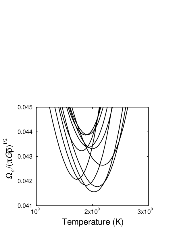
Figure 6.2: Critical angular velocities of realistic $1.4M_{\odot}$ neutron star models, Lindblom et al. [85]

.

6.2 Vorticity-shear viscosity coupling

In spite of the recent improvements in our understanding of the $r$-mode instability, it seems that the fundamental properties of these modes have not yet been sufficiently understood. Previous investigations of the $r$-modes are restricted to the case of uniformly and slowly rotating, isentropic, Newtonian stars [83]. A few recent studies were done for relativistic stars with slowly rotating and Cowling approximations [62]. In this sense, it is interesting to study the properties of the $r$-mode instability in the more general cases, for example, differentially and rapidly rotating, non-isentropic relativistic stars.

In addition, people have used the standard Navier-Stokes theory to study $r$-mode stability enforced by viscosity, and have calculated the corresponding timescales. This theory and its relativistic generalization are non-causal and unstable. An improved causal dissipative fluid theory is based on kinetic theory [18]. This latter theory has implications different from Navier-Stokes theory. For example, kinetic theory predicts that the angular velocity of the star couples to the viscosity and heat flux in rotating stars.

In this section we investigate the possible effect of vorticity-shear viscosity coupling on the stability of $r$-mode and show that the coupling may have a significant effect on viscous damping timescales of $r$-mode [4]. We find that colder stars can remain stable at higher spin rates.

6.2.1 Predicted effect

In standard Navier-Stokes theory the viscous quantities are defined by

$$\Pi=-\zeta\Theta\,,~{}q_{a}=-\kappa\nabla_{a}T\,,~{}\pi_{ab}=-2\eta\sigma_{ab}\,,$$ (6.48)

where $\Pi$ is the bulk viscous stress and $\zeta$ is the bulk viscosity; $q_{a}$ is the heat flux and $\kappa$ is the thermal conductivity; $\pi_{ab}$ is the shear viscous stress and $\eta$ is the shear viscosity; $\Theta=\nabla_{a}v^{a}$ is the volume expansion rate of the fluid, $T$ is the temperature, and $\sigma_{ab}=\nabla_{\langle a}v_{b\rangle}$ is the rate of shear (where the angled brackets denote the symmetric tracefree part). Its is clear that the fluid vorticity $\varpi\varpi\varpi={1\over 2}\nabla\nabla\nabla\,\times\,{\bf v}$ does not enter Eq. (6.48), even when the equilibrium state is rotating.

On physical grounds, one might expect that rotational accelerations can couple with gradients of momentum and temperature, so that there could in principle be couplings of $\varpi_{a}$ to $q_{a}$ and $\pi_{ab}$. In the case of heat flux, qualitative particle dynamics indicates [93] (p. 34) that this coupling does exist as a result of a Coriolis effect, which is in some sense analogous to the Hall effect in a conductor subject to a magnetic field. The Coriolis effect on heat flux is confirmed by molecular dynamics simulations [94]. Müller [95] and Israel & Stewart [18] showed that the Boltzmann equation predicts in general a coupling of vorticity to heat flux and shear viscous stress. The microscopic and self-consistent kinetic approach is in contrast to the continuum view, where a phenomenological principle of “frame indifference” is invoked to argue against any vorticity coupling. (See [93, 94, 96] for further discussion.)

Using the Grad moment method to approximate the hydrodynamic regime via kinetic theory, the relations in Eq. (6.48) are modified to [18] (Eq. (7.1))

$$\Pi = -\zeta\left[\Theta+\beta_{0}\dot{\Pi}\right]\,,$$ (6.49a)

$$q_{a} = -\kappa\left[\nabla_{a}T+T\beta_{1}\left\{\dot{q}_{a}-\varpi_{ab}q^{b}\right\}\right]\,,$$ (6.49b)

$$\pi_{ab} = -2\eta\left[\sigma_{ab}+\beta_{2}\left\{\dot{\pi}_{\langle ab\rangle}-2\varpi^{c}{}_{\langle a}\pi_{b\rangle c}\right\}\right]\,,$$ (6.49c)

where $\beta_{A}$, $A=0,1,2$, can be evaluated in terms of collision integrals for specific gases, an overdot denotes the comoving (Lagrangian) derivative, and the vorticity tensor is given by

$$\varpi_{ab}=\nabla_{[a}v_{b]}=\varepsilon_{abc}\varpi^{c}\,,$$

$$\varpi\varpi\varpi={1\over 2}\nabla\nabla\nabla\,\times\,{\bf v}\,,$$

where square brackets on indices indicate the skew part. Navier-Stokes theory is recovered from the Müller-Israel-Stewart theory when $\beta_{A}=0$. However, kinetic theory gives $\beta_{A}$ values for simple gases which are definitely not zero. Furthermore, if $\beta_{A}=0$, the equilibrium states are unstable and dissipative signals can propagate at unbounded speed [18, 96].

The $\beta_{A}$-corrections will be very small except if there are either high frequency oscillations (pumping up the time-derivative terms) or rapid rotation (pumping up the vorticity-coupling terms). In the context of rapidly rotating neutron stars, we expect the vorticity-dissipative couplings to dominate the time-derivative terms; this expectation is borne out by calculations (see below). The vorticity-dissipative couplings will be negligible if the unperturbed equilibrium state is irrotational, i.e., if $\varpi_{a}=0$ in the background, so that the coupling terms become second-order. However, for fast rotation, $\varpi_{a}\neq 0$ in the background and the coupling terms make a first-order contribution to dissipation. In the words of Israel & Stewart [18]: “these results will ultimately be of practical interest in astrophysical and cosmological situations involving fast rotation, strong gravitational fields or rapid fluctuations (neutron stars, black hole accretion, early universe), although it will probably be some time before the state of the art in these fields makes such refinements necessary.”
We believe that recent and ongoing developments in rotating neutron star physics have reached the stage where the Müller-Israel-Stewart theoretical corrections to the Navier-Stokes equations need to be examined, and our results indicate that the corrections could be important.

We follow the standard assumption [89] that the heat flux may be neglected relative to viscous stresses in calculating damping timescales. Then the vorticity correction to Navier-Stokes theory reduces to the coupling term $\varpi^{c}{}_{\langle a}\pi_{b\rangle c}$. This term means that the angular momentum of the star changes the shear viscosity timescale, and we find (for axial $r$-modes) a correction proportional to $T^{-r}\Omega^{2}$, where $r=9$ for a nonrelativistic fluid and $r=12$ for an ultrarelativistic fluid.

Replacing $\delta\sigma$ and $\delta\sigma_{ab}$ by $\delta\Pi$ and $\delta\pi_{ab}$ in Eq. (6.33), respectively, the evolution of dissipation energy contained in small fluctuations is given by

$$\frac{d\tilde{E}}{dt}=-\int\left({\delta\Pi\delta\Pi^{*}\over\zeta}+{\delta\pi^{ab}\delta\pi_{ab}^{*}\over 2\eta}\right)d^{3}x-\left(\frac{d\tilde{E}}{dt}\right)_{\!\rm\sc gr}\,,$$ (6.50)

where $(d\tilde{E}/dt)_{\rm\sc gr}$ is the energy flux in gravitational radiation (see Eq. (6.33)), $\delta\Pi=\Pi-\bar{\Pi}$ and $\delta\pi_{ab}=\pi_{ab}-\bar{\pi}_{ab}$, with an overbar denoting background quantities. In this case, $\bar{\Pi}=0=\bar{\pi}_{ab}$. The normal modes of the star are damped by dissipation, and the damping rate can be determined by Eq. (6.50). For a normal mode with time dependence $e^{i\omega t}$, the energy has time dependence $\exp[-2{\rm Im}(\omega)t]$. Then by Eq. (6.50), the characteristic damping time $\tau=1/{\rm Im}(\omega)$ of the fluid perturbation is given by

$$\frac{1}{\tau}=-{1\over 2\tilde{E}}{d\tilde{E}\over dt}=\frac{1}{\tau_{\rm\sc bv}}+\frac{1}{\tau_{\rm\sc sv}}+\frac{1}{\tau_{\rm\sc gr}}\,,$$ (6.51)

where $\tau_{\rm\sc bv}$, $\tau_{\rm\sc sv}$, and $\tau_{\rm\sc gr}$ are the bulk viscous, shear viscous, and gravitational radiation timescales respectively.

To evaluate the vorticity-corrected shear viscous timescale, we use Eq. (6.49c) in Eqs. (6.50) and (6.51). To lowest order

$$\delta\pi_{ab}=-2\eta\left[\delta\sigma_{ab}-2i\omega\eta\beta_{2}\delta\sigma_{ab}+4\eta\beta_{2}\delta\sigma^{c}_{\left<a\right.}\varpi_{\left.b\right>c}\right]\,,$$

where $\varpi_{a}$ is the background vorticity (the background shear vanishes). Then

$$\delta\pi^{ab}\delta\pi^{*}_{ab} = 4\eta^{2}\left\{\delta\sigma^{ab}\delta\sigma^{*}_{ab}+4\gamma^{2}\left[\omega^{2}\delta\sigma^{ab}\delta\sigma^{*}_{ab}\right.\right.$$

$$\left.\left.{}+4\left(\delta\sigma^{ab}\delta\sigma^{*}_{ab}\varpi^{c}\varpi_{c}-\delta\sigma^{ca}\delta\sigma^{*}_{da}\varpi_{c}\varpi^{d}\right)\right]\right\}\,,$$

where $\gamma=\eta\beta_{2}$. The first term is the usual term in Navier-Stokes theory, while the following terms are the Müller-Israel-Stewart corrections. The $\omega^{2}$ term arises from $\dot{\pi}_{ab}$ in Eq. (6.49c), and is negligible relative to the $\varpi^{2}$ terms which arise from the $\varpi^{c}{}_{\langle a}\pi_{b\rangle c}$ term in Eq. (6.49c). The energy dissipation rate through shear viscosity will be

$$\left(\!\frac{d\tilde{E}}{dt}\!\right)_{\!\!\rm\sc sv} = -2\!\int\!\eta\left\{\delta\sigma^{ab}\delta\sigma^{*}_{ab}-4\gamma^{2}\left[\omega^{2}\delta\sigma^{ab}\delta\sigma^{*}_{ab}\right.\right.$$ (6.52)

$$\left.\left.{}+4\left(\delta\sigma^{ab}\delta\sigma^{*}_{ab}\varpi^{c}\varpi_{c}-\delta\sigma^{ca}\delta\sigma^{*}_{da}\varpi_{c}\varpi^{d}\right)\right]\right\}d^{3}x.$$

In order to proceed further, we need expressionx for the shear viscosity $\eta$ and the coupling coefficient $\beta_{2}$. For the various interactions, $\eta(\rho,T)$ is calculated in [97, 98], where it is shown that electron-electron scattering is more important for shear viscosity than other interactions. The expression for $\eta$ is given in [89], in good agreement with [97, 98], as

$$\eta=1.10\times 10^{16}\left(\!{\rho\over 10^{14}{\rm g/cm}^{3}}\!\right)^{\!9/4}\left(\!{10^{9}{\rm K}\over T}\!\right)^{\!2}\rm{g/cm\,s}\,.$$ (6.53)

For a Maxwell-Boltzmann gas, the coefficient $\beta_{2}$ is found in [18], but we require the expression for a degenerate Fermi gas. This has been found by Olson & Hiscock [99] in the case of strong degeneracy:

$$\beta_{2}={15\pi^{2}\hbar^{3}\over m^{4}gc^{5}}\frac{(1+\nu)}{(\nu^{2}+2\nu)^{5/2}}+{\cal O}\left[\left({kT\over mc^{2}\nu}\right)^{\!2}\right]\,,$$ (6.54)

where $m$ is the particle mass, $g$ is the spin weight, and $mc^{2}\nu/kT\gg 1$. The dimensionless thermodynamic potential $\nu=(\rho+p)/nm-mc^{2}s/kT-1$, where $s$ is the specific entropy, is equal to the nonrelativistic chemical potential per particle divided by the particle rest energy. For a strongly degenerate gas, the nonrelativistic chemical potential is proportional to $T$, so that

$$\nu\approx{\bar{\alpha}}\,{kT\over mc^{2}}\,,$$

where ${\bar{\alpha}}\gg 1$ is a dimensionless constant measuring the degree of degeneracy. The nonrelativistic regime is obtained for $\nu\ll 1$, while the ultrarelativistic case corresponds to $\nu\gg 1$.

For temperatures below $10^{10}$ K, neutrons in the neutron star are nonrelativistic, while electrons are ultrarelativistic [97]. The nonrelativistic limit of $\beta_{2}$ is

$$(\beta_{2})_{{\rm\sc nr}}\approx 3.16\times 10^{-5}({\bar{\alpha}}T)^{-5/2}~{}\mbox{cm s}^{2}/\rm{g}\,,$$ (6.55)

and its ultrarelativistic limit is

$$(\beta_{2})_{{\rm\sc ur}}\approx 6.45\times 10^{15}({\bar{\alpha}}T)^{-4}~{}\mbox{cm s}^{2}/\rm{g}\,.$$ (6.56)

Using Eqs. (6.53), (6.55) and (6.56), we have

$$\gamma_{{\rm\sc nr}}\approx{1.10\times 10^{-11}\over{\bar{\alpha}}^{5/2}}\left(\!{\rho\over 10^{14}{\rm g/cm}^{3}}\!\right)^{\!9/4}\left(\!{10^{9}{\rm K}\over T}\!\right)^{\!9/2}\rm{s}\,,$$ (6.57)

$$\gamma_{{\rm\sc ur}}\approx{7.08\times 10^{-5}\over{\bar{\alpha}}^{4}}\left(\!{\rho\over 10^{14}{\rm g/cm}^{3}}\!\right)^{\!9/4}\left(\!{10^{9}{\rm K}\over T}\!\right)^{\!6}\rm{s}\,.$$ (6.58)

In these calculations, we have used the same relation for $\eta$ in both cases, because in the high-density regime ($\rho>10^{14}$g/ cm³) for both electron-electron scattering and electron-neutron scattering, $\eta$ is proportional to $T^{-2}$, with nearly equal proportionality factor [97]. For typical values of the temxerature, $T=10^{9}$ K, and density, $\rho=3\times 10^{14}$ g/cm³, we find that $\gamma_{{\rm\sc ur}}\sim{\bar{\alpha}}^{-4}\times 10^{-4}$ s, while $\gamma_{{\rm\sc nr}}\sim{\bar{\alpha}}^{-5/2}\times 10^{-10}$ s.

6.2.2 $r$-mode instability curve

In this section we calculate the predicted effect, Eq. (6.52), for the $r$-mode instability. We assume that the background is a uniformly rotating star, so that the equilibrium fluid velocity is $v^{a}=\Omega\phi^{a}$, where $\phi^{a}$ is the rotational Killing vector field [100]. The vorticity vector of the equilibrium state is

$$\varpi\varpi\varpi=\frac{\Omega}{2r}\left[\cot\vartheta\,,-1\,,0\right]\,.$$ (6.59)

The $r$-modes of rotating barotropic Newtonian stars have Eulerian velocity perturbations given by Eq. (6.18)

$$\delta{\bf v}=\alpha R\Omega\left(\frac{r}{R}\right)^{\ell}{\bf Y}^{B}_{\ell\ell}\exp(i\omega t)\,,$$ (6.60)

where $C$ is an arbitrary constant, $R$ is the unperturbed stellar radius, and $\omega=2\Omega/(\ell+1)$. The magnetic-type vector spherical harmonics ${\bf Y}^{B}_{\ell m}$ are defined by

$${\bf Y}^{B}_{lm}=\frac{r}{\sqrt{\ell(\ell+1)}}\nabla\nabla\nabla\times\left[r\nabla\nabla\nabla Y_{\ell m}(\vartheta,\varphi)\right]\,.$$ (6.61)

The shear of the perturbed star is given by

$$\delta\sigma_{ab}=\nabla_{\langle a}\delta v_{b\rangle}\,.$$ (6.62)

Substituting Eqs. (6.59)–(6.62) into Eq. (6.52), we find the shear viscosity timescale for $\ell=m$:

$$\frac{1}{\tau_{\rm s}}\approx Q_{\ell}\left[(\ell-1)(2\ell+1)\int^{R}_{0}\eta r^{2\ell}\,dr+\Omega^{2}{\cal S}_{\ell}\right]\,,$$ (6.63)

where $Q_{\ell}^{-1}=\int_{0}^{R}\rho r^{2\ell+2}\,dr$. The first term in brackets is in agreement with the expression calculated in [77], and ${\cal S}_{\ell}$ is the correction term:

$${\cal S}_{\ell} \approx 16{(\ell-1)(2\ell+1)\over(\ell+1)^{2}}U_{0}+\frac{\ell(\ell-2)![(2\ell-1)!!]^{2}}{(\ell+1)(2\ell-1)(2\ell)!}\,\frac{\Gamma({{1\over 2}})}{\Gamma(\ell-{{1\over 2}})}\times$$ (6.64)

$${}\times\left[(2\ell^{3}-8\ell^{2}-3\ell-6)U_{2}+12(\ell^{3}-\ell^{2}-\ell+1)U_{3}\right.$$

$$\left.{}+2(4\ell^{4}-\ell^{3}-9\ell^{2}+5\ell+1)U_{4}\right]\,,$$

where $U_{k}(T)\equiv R^{k}\int^{R}_{0}\gamma^{2}~{}\eta r^{2\ell-k}\,dr$.

For the $\ell=2$ modes, Eqs. (6.63) and (6.64) give

$$\frac{1}{\tau_{\rm s}}=5Q_{2}\int^{R}_{0}\eta r^{4}\,dr\,+{\textstyle{1\over 9}}Q_{2}\Omega^{2}\left[80U_{0}+93U_{2}+54U_{3}-42U_{4}\right]\,.$$ (6.65)

For comparison with previous calculations based on Navier-Stokes viscosity (see, e.g., [85]), we use an $n=1$ polytrope with mass $M=1.4M_{\odot}$ and radius $R=12.53$ km to evaluate the integrals in Eq. (6.65). The bulk viscous and gravitational radiation timescales are unaffected by the vorticity correction, and we obtain

$$\frac{1}{\tau(\Omega,T)}=\frac{1}{\tilde{\tau}_{\rm\sc gr}}\left(\frac{\Omega}{\Omega_{\rm\sc k}}\right)^{6}+\frac{1}{\tilde{\tau}_{\rm\sc bv}}\left(\frac{T}{10^{9}\rm K}\right)^{6}\left(\frac{\Omega}{\Omega_{\rm\sc k}}\right)^{2}$$

$$~{}~{}~{}~{}~{}~{}~{}~{}~{}~{}~{}~{}~{}~{}~{}~{}~{}{}+\frac{1}{\tilde{\tau}_{\rm\sc sv}}\left(\frac{10^{9}\rm K}{T}\right)^{2}\left[1+q{\bar{\alpha}}^{4-r}\left(\!\frac{10^{9}\rm K}{T}\!\right)^{\!r}\!\left(\!\frac{\Omega}{\Omega_{\rm\sc k}}\!\right)^{\!2}\right]\,,$$ (6.66)

where $\Omega_{\rm\sc k}=\sqrt{\pi G\bar{\rho}}$, which is ${3\over 2}$ times the Keplerian (mass-shedding) frequency, and the vorticity correction factors are

$$q=\left\{\begin{array}[]{l}1.36\times 10^{-23}\,,\\ 5.67\times 10^{-10}\,,\end{array}\right.~{}r=\left\{\begin{array}[]{ll}9&{\rm nonrel}\,,\\ 12&{\rm ultrarel}\,.\end{array}\right.$$ (6.67)

The standard result (see, e.g., [85]) is regained for $q=0$, with

$$\tilde{\tau}_{\rm\sc gr}=-3.26\,{\rm s}\,,~{}\tilde{\tau}_{\rm\sc bv}=2.01\times 10^{11}\,{\rm s}\,,~{}\tilde{\tau}_{\rm\sc sv}=2.52\times 10^{8}\,{\rm s}\,.$$

We note that the contribution from the $\dot{\pi}_{ab}$ term in Eq. (6.49c) to the $q$-correction is less than 1% of the contribution from the $\varpi^{c}{}_{\langle a}\pi_{b\rangle c}$ term.

Now we are able to determine from Eq. (6.66) the critical angular velocity $\Omega_{\rm\sc c}$, defined by $1/\tau(\Omega_{\rm\sc c},T)=0$, which governs stability of the star: if $\Omega>\Omega_{\rm\sc c}$, then dissipative damping cannot overcome the gravitational radiation-driven instability. In Fig. 6.3 we plot $\Omega_{\rm\sc c}/\Omega_{\rm\sc k}$ against temperature $T$, showing how the vorticity-viscosity coupling affects the standard result (see, e.g., [85]). Electrons are assumed to dominate the shear viscosity, and they are ultrarelativistic over the range of temperatures.

It is clear from Fig. 6.3 that the vorticity correction is only appreciable at temperatures $T\leq 10^{8}$ K, but that for these lower temperatures, the correction can be large, especially for smaller ${\bar{\alpha}}$. As the degree of degeneracy increases (i.e., with increasing ${\bar{\alpha}}$), the correction is confined to lower and lower temperatures. The effect of the vorticity-viscosity coupling is to increase the stable region, so that cooler stars can spin at higher rates and remain stable. This may modify recent results [101] which suggest that $r$-mode instability could stall the spin-up of accreting neutron stars with $T\geq 2\times 10^{5}$ K; if the vorticity correction operates, then the stability region is increased, so that spin-up could be more effective, especially for lower degeneracy parameter ${\bar{\alpha}}$.

We note that, here, we have used for our $r$-mode calculations solutions that assume slow rotation. Thus the $\Omega/\Omega_{\rm\sc k}\geq 0.3$ part of Fig. 6.3 is an extrapolation to high spin rates, in common with previous stability diagrams. Recent calculations of $r$-modes for rapid rotation [88] should be used in future calculations of the vorticity correction. Since $f$-modes are unstable at high spin rate, the effect of the vorticity correction on these modes would also be interesting to calculate.

Figure 6.3: Critical angular velocity versus temperature ($n=1$ polytrope with mass 1.4$M_{\odot}$ and radius 12.57 km). The stability region is below the curves. The solid curve shows the standard result, with no coupling of viscosity to vorticity. Broken curves (labelled by the degeneracy parameter ${\bar{\alpha}}$) show how the instability region is reduced by the kinetic-theory coupling of shear viscosity to vorticity, for an ultra-relativistic degenerate Fermi fluid (electron-electron viscosity).

6.3 Post-glitch relaxation of Crab

As we discussed before, the $r$-mode instability opens a wide window for gravitational wave astronomy. It would give us some information about the interior matter of neutron stars. Determining cooling rates, viscosity, crust formation, the equation of state of neutron matter, the onset of superfluidity in neutron stars, and several other features of neutron stars are more interesting implications of this instability. In this section, we discuss one of possible $r$-mode implications.

More than 30 years after the discovery of the pulsar phenomenon and its identification with neutron stars, there exists still a number of uncertainties and open questions about the theoretical model for pulsars, mainly due to the extremely dense state of matter in neutron stars. During the past two decades, the glitch phenomenon, a sudden increase of angular velocity of the order of $\Delta\Omega/\Omega\leq 10^{-6}$, and the very long relaxation times, from months to years, after the glitch, remain as one of the great mysteries of pulsars. The observed post-glitch relaxation of the Crab pulsar has been unique in that the rotation frequency of the pulsar is seen to decrease to values $less$ than its pre-glitch extrapolated values. So far, two mechanisms have been suggested to account for the observed excess loss of angular momentum during post-glitch relaxations of the Crab. The first mechanism, in the context of the vortex creep theory of Alpar et al. [102, 103], invokes generation, at a glitch, of a so called “capacitor” region within the pinned superfluid in the crust of a neutron star, resulting in a permanent decoupling of that part of the superfluid. Neverthless, this suggestion has been disqualified (Lyne et al. [104]) since the moment of inertia required to have been decoupled permanently in such regions during the past history of the pulsar is found to be much more than that permitted for all of the superfluid component in the crust of a neutron star. In another attemp, Link et al. [105] have attributed the excess loss of angular momentum to an increase in the electromagnetic braking torque of the star, as a consequence of a sudden increase, at the glitch, in the angle between its magnetic and rotation axes. As they point out, such an explanation is left to future observational verification since it should also accompany other observable changes in the pulsar emission, which have not been detected, so far, in any of the resolved glitches in various pulsars. Moreover, the suggestion may be questioned also on the account of its long-term consequences for pulsars, in general. Namely, the inclination angle would be expected to show a correlation with the pulsar age, being larger in the older pulsars which have undergone more glitches. No such correlation has been deduced from the existing observational data. Also, and even more seriously, the assumption that the braking torque depends on the inclination angle is in sharp contradiction with the common understanding of pulsars spin-down process. The currently inferred magnetic field strengths of all radio pulsars are in fact based on the opposite assumption, namely that the torque is independent of the inclination angle. The well-known theoretical justification for this, following Goldreich & Julian [106], is that the torque is caused by the combined effects of the magnetic dipole radiation and the emission of relativistic particles, which compensate each other for the various angles of inclination (see, eg., Manchester & Taylor [107]; Srinivaran [108]).

The excitation of r-modes at a glitch and the resulting emission of gravitational waves could, however, account for the required “sink” of angular momentum in order to explain the peculiar post-glitch relaxation behavior of the Crab pulsar. As is shown in Figs. 6.4 and 6.5, for values of $\alpha_{0}\geq 0.04$ the predicted time evolution of $\Delta\Omega\over\Omega$ and $\Delta\dot{\Omega}\over\dot{\Omega}$ during the 3–5 years of the inter-glitch intervals in Crab, might explain the observations. That is, the predicted total change in the rotation frequency of the star, $|{\Delta\Omega\over\Omega}|$, is much larger than the corresponding jump $\frac{\Delta\Omega}{\Omega}\sim 10^{-8}$ at the glitch, which explains why the post-glitch values of $\Omega$ should fall below that expected from an extrapolation of its pre-glitch behavior. Also, the predicted values of ${\Delta\dot{\Omega}\over\dot{\Omega}}\sim 10^{-4}$, after a year or so (Fig. 6.5), are in good agreement with the observed persistent shift in the spin-down rate of the Crab (Lyne et al. [109]).

The predicted increase in the spin-down rate would be however diminished as the excited modes at a glitch are damped out, leaving a permanent negative offset in the spin frequency. Hence the above so-called persistent shift in the spin-down rate of the Crab may be explained in terms of the effect of r-modes, as long as it persists during the inter-glitch intervals of 2-3 years. It may be noted that a really persistent shift in the spin-down rate at a glitch may be caused by a sudden decrease in the moment of inertia of the star. However this effect, by itself, could not result in the observed negative offset in the spin frequency.

The same mechanism would be expected to be operative during the post-glitch relaxation in the other colder and slower pulsars, as well. However, for the similar values of $\alpha_{0}$, ie. the same initial amplitude of the excited modes, the effect is not expected to become “visible” in the older pulsars. Particularly, for the Vela its initial jump in frequency at a glitch, $\frac{\Delta\Omega}{\Omega}\sim 10^{-6}$, is seen from Fig. 6.4 to be much larger (ie. by some four orders of magnitudes) than that of the above effect due to the r-modes. In other words, while the predicted loss in the stellar angular momentum due to the excitation of r-modes result in a negative $\Delta\Omega\over\Omega$ which, in the case of Crab, overshoots the initial positive jump at a glitch, however for the Vela and older pulsars it comprises only a negligible fraction of the positive glitch-induced jump. A more detailed study should, however, take into account the added complications due to internal relaxation of various components of the star, which is highly model dependent. The observed initial rise in $\Omega$ need not be totally compensated for by the losses due to r-modes which we have discussed, since part of it could be relaxed internally (by a transfer of angular momentum between the “crust” and other components, and/or temporary changes in the effective moment of inertia of the star) even in the absence of any real sink for the angular momentum of the star. Such considerations would not only leave the above conclusions valid but also allow for even smaller values of the initial amplitude of the excited modes, compared to our presently adopted value of $\alpha_{0}\sim 0.04$.

The suggested effect of the r-modes in the post-glitch relaxation of pulsars should be understood as one operating in addition to that of the internal relaxation which is commonly invoked. While the latter could account only for a relaxation back to the extrapolated pre-glitch values of the spin frequency, the additional new effect due to the r-modes may explain the excess spin-down observed in the Crab pulsar as well.

It is further noted that the above estimates are for an adopted value of $Q=9.4\times 10^{-2}$, which corresponds to the particular choice of the polytropic model star. Differences in the structure among pulsars, in particular between Crab and Vela, which have also been invoked in the past (see, eg., Takatsuka & Tamagaki [110]), could be further invoked to find a better agreement with the data for the above effect due to r-modes as well. Also, the initial amplitude of the excited modes need not be the same in all pulsars. It is reasonable to assume that in a hotter and faster rotating neutron star, as for the Crab, larger initial amplitudes, ie. larger values of $\alpha_{0}$, are realized than in the colder–slower ones.

6.3.1 Predicted Effect

In order to estimate the effect of the $r$-mode instability, in a “stable” neutron star, on its post-glitch relaxation, we have used the model described by Owen et al. [81]. The total angular momentum of a star is parameterized in terms of the two degrees of freedom of the system. One, is the uniformly rotating equilibrium state which is represented by its angular velocity $\Omega_{\rm eq}$. The other, is the excited $r$-mode that is parameterized by its magnitude $\alpha$ which is bound to an upper limiting value of $\alpha=1$, in the linear approximation regime treated in the model. Thus, the total angular momentum $J$ of the star is written as a function of the two parameters $\Omega_{\rm eq}$ and $\alpha$:

$$J=I_{\rm eq}\Omega_{\rm eq}+J_{c},$$ (6.68)

where $I_{\rm eq}=\tilde{I}MR^{2}$ is the moment of inertia of the equilibrium state, and $J_{c}=-{3\over 2}\tilde{J}\alpha^{2}\Omega_{\rm eq}MR^{2}$ is the canonical angular momentum of the $l=2$ $r$-mode, which is negative in the rotating frame of the equilibrium star. The dimensionless constants

$$\tilde{I}={8\pi\over 3MR^{2}}\int_{0}^{R}\rho r^{4}\,dr$$ (6.69)

$$\tilde{J}={1\over MR^{4}}\int_{0}^{R}\rho r^{6}\,dr,$$ (6.70)

depend on the detailed structure of the star, and for the adopted $n=1$ polytropic model considered have values $\tilde{I}=0.261$ and $\tilde{J}=0.01635$. Also $R=12.54$ km and $M=1.4\ M_{\odot}$ are the assumed radius and mass of the star, for the same polytropic model.

Eq. (6.68) above implies that an assumed instantaneous excitation of $r$-modes at a glitch would cause a sudden increase in $\Omega_{\rm eq}$. For definiteness, we define the “real” observable rotation frequency $\Omega$ of the star as $\Omega={J\over I}$, where $I$ is the moment of inertia of the real star. The two are equal, $\Omega=\Omega_{\rm eq}$, in the absence of the $r$-modes, ie. before the excitation of the modes at a glitch and after the modes are damped out. If there were no loss of angular momentum (by gravitational radiation) accompanying the post-glitch damping of the modes (by viscosity) $\Omega_{\rm eq}$ would recover its extrapolated pre-glitch value; ie. its initial rise would be compensated exactly. However due to the net loss of angular momentum by the star, the post-glitch decrease of $\Omega_{\rm eq}$ overshoots its initial rise. The negative offset between values of $\Omega_{\rm eq}$ before the excitation of the modes and after they are damped out is the quantity of interest for our discussion. The question of whether the instantaneous rise in the value of $\Omega_{\rm eq}$ at a glitch, due to the excitation of the $r$-modes, is observable or not is a separate problem, and its resolution would have no consequence for the net loss of angular momentum from the star which is the relevant quantity here. It is noted that the distinction between $\Omega$ and $\Omega_{\rm eq}$, in the presence of modes, is quantitatively negligible, in all cases of interest, and is usually disregarded. Also, one might dismiss an increase in $\Omega_{\rm eq}$ as implied by Eq. (6.68) to be observable as a spin-up of the star since for an inertial outside observer the $r$-modes rotate in the prograde direction and their excitation should result, if at all, in a spin-down of the star. Moreover, an excitation of the $r$-modes should not result, by itself, in any real change of the rotation frequency of the star at all. Because one could not distinguish two physically separate parts of the stellar material such that the two components of angular momentum in Eq. (6.68) may be assigned to the two parts separately.

The total angular momentum $J$ of the star in terms of $\Omega_{eq}$ and $\alpha$ is

$$J(\Omega_{\rm eq},\alpha)=\left({\tilde{I}}-{3\over 2}{\tilde{J}}\alpha^{2}\right)\Omega_{\rm eq}MR^{2}.$$ (6.71)

The perturbed star loses angular momentum primarily through the emission of gravitational radiation. Thus, the evolution of $J(\Omega_{\rm eq},\alpha)$ can be computed by using the standard multipole expression for angular momentum loss. Then, for the $\ell=m=2$ case

$${dJ\over dt}=-{c^{3}\over 16\pi G}\left({4\Omega_{\rm eq}\over 3}\right)^{5}(S_{22})^{2},$$ (6.72)

where $c$ is the speed of light and $\ell=m=2$ current multipole, $S_{22}$, is given by [91]

$$S_{22}=\sqrt{2}{32\pi\over 15}{GM\over c^{5}}\alpha\Omega_{\rm eq}R^{3}{\tilde{J}}.$$ (6.73)

Combining Eq. (6.72) for the angular momentum evolution of the star with Eqs. (6.42) and (6.73), we obtain one equation for the evolution of the parameters $\Omega_{\rm eq}$ and $\alpha$ that determine the state of the star:

$$\left({\tilde{I}}-{3\over 2}{\tilde{J}}\alpha^{2}\right){d\Omega_{\rm eq}\over dt}-3\alpha\Omega_{\rm eq}{d\alpha\over dt}={3\alpha^{2}\Omega_{\rm eq}{\tilde{J}}\over\tau_{\rm\sc gr}}.$$ (6.74)

In addition to radiating angular momentum from the star via gravitational radiation, the mode will also lose energy through gravitational radiation and neutrino emission (from bulk viscosity). Furthermore the mode energy is deposited into the thermal state of the star by shear viscosity. Therefore the energy balance equation should be considered together with Eq. (6.74) to determine the parameters $\Omega_{\rm eq}$ and $\alpha$. For the $\ell=2$ $r$-mode $\tilde{E}$, Eq. (6.39), is given by

$${\tilde{E}}={\scriptstyle\frac{1}{2}}\alpha^{2}\Omega^{2}_{\rm eq}MR^{2}{\tilde{J}}.$$ (6.75)

The time derivative of $\tilde{E}$, Eq. (6.51), is

$${d\tilde{E}\over dt}=-2{\tilde{E}}\left(\frac{1}{\tau_{\rm\sc v}}+\frac{1}{\tau_{\rm\sc gr}}\right)\,,$$ (6.76)

where $\tau_{\rm\sc v}$ and $\tau_{\rm\sc gr}$ are the viscous and gravitational radiation timescales respectively. Combining Eqs. (6.75) and (6.76), the second evolution equation for $\Omega_{\rm eq}$ and $\alpha$ is given by

$$\Omega_{\rm eq}{d\alpha\over dt}+\alpha{d\Omega_{\rm eq}\over dt}=-\alpha\Omega_{\rm eq}\left(\frac{1}{\tau_{\rm\sc v}}+\frac{1}{\tau_{\rm\sc gr}}\right).$$ (6.77)

Therefore the time evolution of the quantities $\alpha$ and $\Omega_{\rm eq}$ can be determineded from the coupled equations (Owen et al. [81]):

$$\frac{{\rm d}\Omega_{\rm eq}}{{\rm d}t}=-\frac{2\Omega_{\rm eq}}{\tau_{\rm\sc v}}\frac{\alpha^{2}Q}{1+\alpha^{2}Q},$$ (6.78a)

$$\frac{{\rm d}\alpha}{{\rm d}t}=-\frac{\alpha}{\tau_{\rm\sc gr}}-\frac{\alpha}{\tau_{\rm\sc v}}\frac{1-\alpha^{2}Q}{1+\alpha^{2}Q},$$ (6.78b)

where $Q={3\over 2}{\tilde{J}\over\tilde{I}}=0.094$, for the adopted equilibrium model of the star. The viscous time has two contributions from the shear and bulk viscousities with corresponding timesacels $\tau_{\rm sv}$ and $\tau_{\rm bv}$, respectively. The overall “damping” timescale $\tau$ for the mode, which is a measure of the period over which the excited mode will persist, is defined as

$$\frac{1}{\tau}=\frac{1}{\tau_{\rm\sc v}}+\frac{1}{\tau_{\rm\sc gr}}=\frac{1}{\tau_{\rm\sc sv}}+\frac{1}{\tau_{\rm\sc bv}}+\frac{1}{\tau_{\rm\sc gr}}$$ (6.79)

Following Owen et al. [81] we use $\tau_{\rm\sc sv}=2.52\times 10^{8}({\rm s})T_{9}^{2}$, $\tau_{\rm\sc bv}=4.92\times 10^{10}({\rm s})T_{9}^{-6}\Omega_{3}^{-2}$, and $\tau_{\rm\sc gr}=-1.15\times 10^{6}({\rm s})\Omega_{3}^{-6}$, where $T_{9}$ is the temperature, $T$, in units of $10^{9}$ K, and $\Omega_{3}$ is in units of $10^{3}{\rm rad\ s}^{-1}$. These estimates do not however include the role of superfluid mutual friction in damping out the oscillations. We have further taken into account the damping due to the mutual friction using the associated damping time as given by Lindblom and Mendell [111]. The effect of the mutual friction is nevertheless seen to be negligible and the computed curves shown below remain almost the same in the presence of mutual friction.

By integrating Eqs. (6.78a) and (6.78b), numerically, for a given initial value of $\alpha$, one may therefore follow the time evolution of $\alpha$ and $\Omega_{\rm eq}$ which together with Eq. (6.68) determine the time evolution of the total angular momentum, $J$, and hence the time evolution of $\Omega$. Figs. 6.4 and 6.5 shows the computed time evolution for the absolute value of the resulting (negative) fractional change $\Delta\Omega\over\Omega$ in the spin frequency (Fig. 6.4) and also the change $\Delta\dot{\Omega}\over\dot{\Omega}$ in the spin-down rate of the star (Fig. 6.5), starting at the glitch epoch which corresponds to time $t=0$. The results in Figs. 6.4 and 6.5 are for a choice of an initial value of $\alpha_{0}=0.04$, and for the assumed values of $T$ and $\Omega$ corresponding to the Crab and Vela pulsars, as indicated. Fig. 6.4 shows that for the same amplitude of the r-modes assumed to be excited at a glitch the resulting loss of angular momentum through gravitational radiation would be much larger in Crab than in Vela, ie. by more than 3 orders of magnitudes. (Note that the curve for Vela in Fig. 6.4 represents the results after being multiplied by a factor of $10^{3}$.) Furthermore, for the adopted choice of parameter values, the magnitude of the corresponding decrease in $\Omega$ for the Crab, is $|{\frac{\Delta\Omega}{\Omega}}|\sim 10^{-7}$ (Fig. 6.4). The observational consequence of such an effect would nevertheless be closely similar to what has been already observed during the post-glitch relaxations of, only, the Crab pulsar.

Before proceeding further with Crab, we note that the post-glitch effects of excitation of r-modes would however have not much observational consequences for the Vela, and even more so for the older pulsars, which are colder and rotate more slowly. This has two, not unrelated, reasons: in the older pulsars r-modes a) are damped out faster (ie. have smaller values of $\tau$), and b) result in less gravitational radiation. The dependence of $\tau$ on the stellar interior temperature is shown in Fig. 6.6. For the colder, i.e. older, neutron stars the r-modes are expected to die out very fast. The damping timescale for a pulsar with a period $P\sim 1{\rm s}$, being colder than $10^{8}$ K, could be as short as a few hours (Fig. 6.6), and r-modes would have been died out at times longer than that after a glitch. For the hot Crab pulsar, on the other hand, r-modes are expected to persist for 2-3 years after they are excited, say, at a glitch. The value of $\tau$ decreases for older pulsars due to both their longer periods as well as lower temperatures, but the effect due to the latter dominates by many orders of magnitudes, for the standard cooling curves of neutron stars (Urpin et. al. [112]). The second reason, ie. the loss of angular momentum being negligible in older pulsars, was already demonstrated in Fig. 6.4, by a comparison between Crab and Vela pulsars. We have verified it also for the case of pulsars older than Vela. It may be also demonstrated analytically from Eqs. (6.78a) and (6.78b), in the limit of $\alpha^{2}Q<<1$. The initial increase in $\Omega_{\rm eq}$ due to excitation of r-modes with a given initial amplitude $\alpha_{0}$ is seen from Eq. (6.68) to be $|{\Delta\Omega_{\rm eq}\over\Omega_{\rm eq}}|_{0}=\alpha_{0}^{2}Q$. The subsequent damping of the modes result in secular decrease in $\Omega_{\rm eq}$, and the total decrease at large $t\rightarrow\infty$ would be $|{\Delta\Omega_{\rm eq}\over\Omega_{\rm eq}}|_{\infty}\sim{\tau\over\tau_{\rm\sc v}}\alpha_{0}^{2}Q$, which is true for $|{\Delta\Omega_{\rm eq}|<<\Omega_{\rm eq}}$. Note that in the absence of gravitational radiation losses (ie. ${1\over\tau_{\rm\sc gr}}=0;\tau=\tau_{\rm\sc v}$) the total decrease would be the same as the initial increase, which is expected for the role of viscous damping alone. The difference between these two changes (total decrease minus initial increase) in $\Omega_{\rm eq}$ would correspond to the total loss of angular momentum from the star, hence to the net decrease in its observable rotation frequency, ie.

$$|{\Delta\Omega\over\Omega}|_{\infty}={\tau_{\rm\sc v}\over|\tau_{\rm\sc gr}|}\alpha_{0}^{2}Q\,,$$ (6.80)

which is valid in the limit of ${\tau_{\rm\sc v}\over|\tau_{\rm\sc gr}|}<<1$. Fig. 6.7 shows the dependence of the quantity ${\tau_{\rm\sc v}\over|\tau_{\rm\sc gr}|}$ on the stellar rotation frequency, and also on its internal temperature. While for the Crab ${\tau_{\rm\sc v}\over|\tau_{\rm\sc gr}|}\sim 10^{-3}$, however its value is much less for the older pulsars, due to both their lower $\Omega$ as well as lower $T$ values. The dependence on the temperature is however seen to be much less than that on the rotation frequency, in contrast to the dominant role of the temperature in determining the value of the total damping time $\tau$, as indicated above. As is seen in Fig. 6.7, for the Vela ${\tau_{\rm\sc v}\over|\tau_{\rm\sc gr}|}<10^{-7}$, which means a maximum predicted value of $|{\Delta\Omega\over\Omega}|_{\infty}<10^{-8}$, even for the large values of $\alpha_{0}\sim 1$. This has to be contrasted with the glitch induced values of $|{\Delta\Omega\over\Omega}|\sim 10^{-6}$ in Vela, which shows the insignificance of the role of r-modes in its post-glitch behaviour.

Figure 6.4: The post-glitch time evolution of the spin frequency of a pulsar, caused by its loss of angular momentum due to gravitational waves driven by the r-modes that are assumed to be excited at the glitch epoch, $t=0$, with an initial amplitude of $\alpha_{0}=0.04$. The two curves correspond to assumed values of $T_{9}=0.3$ and $\Omega_{3}=0.19$, for the Crab (thick line), and $T_{9}=0.2$ and $\Omega_{3}=0.07$, for the Vela (thin line). Note that the curve for Vela represents the results after being multiplied by a factor of $10^{3}$.

Figure 6.5: Time evolution of the spin-down rate of a pulsar, caused by its loss of angular momentum due to the excitation of r-modes at $t=0$. A value of $\dot{\Omega}=2.4\times 10^{-9}$rad s^-2, and other parameter values same as in Fig. 6.4 for the Crab have been assumed.

Figure 6.6: Dependence of the total damping timescale of r-modes on the internal temperature of a neutron star. Parameter values same as for the Crab in Fig. 6.4 have been assumed.

Figure 6.7: Dependence of the net post-glitch decrease in the rotation frequency, on the rotation frequency of a neutron star. The two curves are to show the dependence on the temperature, where $T_{9}=0.3$ (bare line) and $T_{9}=0.2$ (dotted line) have been used.

Chapter 7 Concluding remarks

In many cosmological and astrophysical situations, an idealized fluid model of matter is inappropriate, and a self-consistent microscopic model based on relativistic kinetic theory gives a more detailed physical description. Kinetic theory offers a microscopic approach to describe the macroscopic features of matter, rather than the phenomenological fluid dynamics and its associated thermodynamics. Starting from a microscopic approach, to obtain an effective macroscopic description, is the most fascinating feature of this theory. The theory is based on a simple function which is called the distribution function which is a solution of Boltzmann’s or Liouville’s equation, and describes the dynamics of the system at the microscopic level. At the macroscopic level, the mass density, flow density, pressure, and the other macroscopic quantities are obtained from the distribution function. On the other hand, observations at large scales, such as stellar systems, can help us to improve our understanding of microphysics.

In chapter 3, general relativistic Liouville’s equation in the post-Newtonian approximation was studied. In the static case, the equilibrium, two static solutions of the Liouville’s equation in this approximation are obtained. These integrals are generalizations of the classical energy, $E={1\over 2}v^{2}+\phi+(2\phi^{2}+\psi)/c^{2}$, and angular momentum, $l_{i}=\varepsilon_{ijk}x^{j}v^{k}\exp(-\phi/c^{2})$. In this spirit, the polytropic model, a simple model for a neutron star, was studied. Our results show that the post-Newtonian corrections tend to reduce the radius of any polytrope. This is a consequence of the fact that the post-Newtonian correction is more significant for systems with larger density [1].

Linear perturbations of phase space distribution functions was investigated in chapter 4. We introduced the linearized Liouville-Einstein equation in this approximation. We showed that, if the underlying potentials are spherically symmetric, the evolution equation is O(3) symmetric, ie. the linearized Liouville-Einstein operator commutes with the angular momentum operator in phase space, $\varepsilon_{ijk}(x^{j}{\partial\over\partial x^{k}}+v^{j}{\partial\over\partial v^{k}})$. Then the modes can be characterized by a pair of angular momentum eigennumbers, $(j,m)$. The eigenvalues $\omega_{j}$ are, however, $(2j+1)$ fold degenerate.

Furthermore, we showed that the post-Newtonian gravitational potentials may excite some of the neutral modes of the star and that these modes are purely relativistic effects. Using the O(3) property of $pnl$, we proposed distribution functions for perturbations that are functions of classical energy and classical angular momentum, Eqs. (4.18) and (D.8):

$$f_{jm}=Re\;\Lambda_{jm}\;\;;\Lambda_{jm}=af(e,l^{2})J_{+}^{j+m}l_{-}^{j}=bf(e,l^{2})J_{-}^{j-m}l_{+}^{j},$$

Although these functions are neutral in classical approximation, they are not so in $pn$ order. Neutral, here, means to belong to zero frequency modes. The weak $pn$ forces generate a sequence of low frequency modes from such perturbations. In their hydrodynamic behavior, they constitute a sequence of low frequency toroidal modes. There is an oscillatory $g_{0i}$ component of the metric tensor associated with these modes. From a conceptual point of view, they are similar to toroidal modes of slowly rotating fluids generated by Coriolis forces or to the standing Alfven waves of a weakly magnetized fluids [2].

The latter perturbations are analogue of the recent quasi normal modes in relativistic systems believed to have been originated from the perturbations of the space-time metric, gravitational wave modes ($w$-modes). Kokkotas and Schutz [113] first recognized the $w$-modes in a toy model of a finite string (to mimic a fluid) coupled to a semi-infinite one (to substitute the dynamical space-time). Such a system accommodates a family of damped oscillations due to the emission of gravitational wave. Different investigators have proposed different mathematical and numerical schemes to isolate these modes [114]–[120]. They verified that strongly damped ($w$-) modes, due to the space-time metric perturbation, do indeed exist in realistic stellar models.

In chapters 5 and 6, we studied the recent and interesting instability in rotating neutron stars. Recently it has been shown that the instability of perturbations of rotating stars are important during the early history of hot neutron stars. These perturbations are driven by the Coriolis force which is always present in a rotating star and are known as $r$-modes. The instability of these modes cause a rotating neutron star’s rotation rate to slow down, emitting gravitational radiation in the process. This emission of gravitational radiation is important both as a possibly detectable source and as a mechanism to explain the observed spin rate of neutron stars.

It is important to improve our understanding of the various factors that go into $r$-mode stability analysis. One important aspect which has needed further elaboration is the role of dissipation in the fluid. Normally, the fluid’s viscosity is thought to damp out any instability if the star is relatively cool. However, the earliest analyses only considered a model for the viscosity based on the Navier-Stokes theory (which is known to have serious problems, such as faster-than-light propagation of signals).

As a first attempt to include more realistic microphysics, we have considered the role of vorticity on the stability of $r$-modes. This effect is predicted by kinetic theory when the unperturbed equilibrium state is rotating, but is absent in Navier-Stokes theory. In standard Navier-Stokes theory, the angular velocity of the fluid has no effect on viscous stress or heat flux. We calculated the vorticity-shear viscosity coupling and showed that the coupling between vorticity and shear viscous stress predicted by kinetic theory can in principle have a significant effect on $r$-mode instability in neutron stars. The Müller-Israel-Stewart correction of Navier-Stokes theory predicts that colder stars can remain stable at higher spin rates, so that accreting spin-up could be protected from $r$-mode instability [4].

Normally all neutron stars which have been observed are seen to be rotating while showing a slow down of their rotation rate. However, some pulsars, such as the Crab pulsar exhibit glitches, which are brief periods during which their rotation rate suddenly increases. We have studied the role of $r$-modes in the post-glitch relaxation of radio pulsars. We have shown that excitation of the $r$-modes at a glitch may provide a solution to an unsolved observed effect in post-glitch relaxation of the Crab pulsar [3].

Of course, our analysis is limited by the fact that we have followed the standard assumption in viscous stability analysis and ignored superfluid effects that will become important at lower temperatures (see, e.g., [111]). Superfluid “friction” effects are thought to prevent $f$-mode instability, and these effects are likely to be relevant also for $r$-modes. These effects may strongly alter the vorticity correction effect, and the possibility of $r$-modes excitation in the Crab like pulsars ($T\sim 10^{8}$ K).

Appendix A The post-Newtonian approximation

The Einstein field equations are nonlinear, and therefore cannot in general be solved exactly. In most cases, by imposing some symmetries such as time independence, spatial isotropy and/or homogenity, we were able to find some exact solutions, the Schwarzschild and the Freidmann-Robertson-Walker metrics for examples. But we cannot actually make use of the symmetries in all problems. Solar system is the familiar example of non-static and anisotropic case.

In most problems what we need is not to find the exact solutions of the problems, but we need a systematic approximation method to extract the solutions without any assumed symmetry properties of the problem.

The post-Newtonian approximation was historically derived [132, 133, 134], to the study of the problem of motion. But in the last three decades, It is used largely to study dynamics of stellar systems like compact stars and black holes.

In this appendix we introduce the post-Newtonain approximation in details. We follow [42] to present this method.

Consider a system of particles that, like the sun and the planets, are bound together by their mutual attraction. Let ${\bar{M}}$, ${\bar{r}}$, and ${\bar{v}}$ be typical values of the masses, separations, and velocities of these particles. The Newtonian typical kinetic energy ${\bar{M}}{\bar{v}}^{2}/2$ will be roughly of the same order of magnitude as the typical potential energy $G{\bar{M}}/{\bar{r}}$, so

$${\bar{v}}^{2}\approx\frac{G{\bar{M}}}{{\bar{r}}}.$$ (A.1)

The relation will be exact for a particle moves with velocity ${\bar{v}}$ in circular orbit of radius ${\bar{r}}$ about a central mass ${\bar{M}}$. The post-Newtonian approximation may be described as a method for obtaining the motion of the system to one higher power of the small parameters $G{\bar{M}}/{\bar{r}}$ and ${\bar{v}}^{2}$ than given by Newtonian mechanics. It is also referred to as an expansion in inverse powers of the speed of light, $c$. Here we prefer to use ${\bar{v}}/c$ as the expansion parameter.

From our experience with the Schwarzschild solution, we expect that it should be possible to find a coordinate system in which the metric tensor is nearly equal to the Minkowski tensor $\eta_{\mu\nu}$, the corrections being expandable in powers of ${\bar{v}}/c$. In particular, we expect

$$g_{oo}=-1+\;^{2}g_{oo}+\;^{4}g_{oo}+\cdots,$$ (A.2a)

$$g_{ij}=\delta_{ij}+\;^{2}g_{ij}+\;^{4}g_{ij}+\cdots,$$ (A.2b)

$$g_{oi}=\;^{3}g_{oi}+\;^{5}g_{oi}+\cdots,$$ (A.2c)

where the symbol ${}^{N}g_{\mu\nu}$ denotes the term in $g_{\mu\nu}$ of order $({\bar{v}}/c)^{N}$. Odd powers of ${\bar{v}}/c$ occur in $g_{io}$ because $g_{io}$ must change sign under time-reversal transformation $t\rightarrow-t$. These expansion lead to a consistent solution of Einstein field equations. The inverse of the metric tensor is defined by the equation

$$g^{i\mu}g_{o\mu}=g^{io}g_{oo}+g^{ij}g_{oj}=0,$$ (A.3a)

$$g^{o\mu}g_{o\mu}=g^{oo}g_{oo}+g^{oi}g_{oi}=1,$$ (A.3b)

$$g^{i\mu}g_{j\mu}=g^{io}g_{jo}+g^{ik}g_{jk}=\delta_{ij}.$$ (A.3c)

We expect that

$$g^{oo}=-1+\;^{2}g^{oo}+\;^{4}g^{oo}+\cdots,$$ (A.4a)

$$g^{ij}=\delta_{ij}+\;^{2}g^{ij}+\;^{4}g^{ij}+\cdots,$$ (A.4b)

$$g_{oi}=\;^{3}g^{oi}+\;^{5}g^{oi}+\cdots,$$ (A.4c)

and inserting these expansions into the Eqs. (A.3), we find

$${}^{2}g^{oo}=-\;^{2}g_{oo};\;\;^{2}g^{ij}=-\;^{2}g_{ij};\;\;^{3}g^{oi}=\;^{3}g_{oi}.$$ (A.5)

The affine connection may be obtained from the familiar formula

$$\Gamma^{\lambda}_{\mu\nu}=\frac{1}{2}g^{\lambda\rho}\left(\frac{\partial g_{\mu\rho}}{\partial x^{\nu}}+\frac{\partial g_{\nu\rho}}{\partial x^{\mu}}-\frac{\partial g_{\mu\nu}}{\partial x^{\rho}}\right).$$ (A.6)

In computing $\Gamma^{\lambda}_{\mu\nu}$ we must note that the scales of distance and time, ${\bar{r}}$ and ${\bar{r}}/{\bar{v}}$, respectively. So the space and time derivatives should be regarded as being of order

$$\frac{\partial}{\partial x^{i}}\approx\frac{1}{\bar{r}};\;\;\frac{\partial}{c\partial t}\approx\frac{\bar{v}/c}{\bar{r}}.$$

Using the metric expansions we find that the various components of $\Gamma^{\lambda}_{\mu\nu}$ have the expansions

$$\Gamma^{\lambda}_{\mu\nu}=\;^{2}\Gamma^{\lambda}_{\mu\nu}+\;^{4}\Gamma^{\lambda}_{\mu\nu}+\cdots;\;\;\;(\rm{for}\;\Gamma^{i}_{oo},\;\Gamma^{i}_{jk},\;\Gamma^{o}_{oi}),$$ (A.7a)

$$\Gamma^{\lambda}_{\mu\nu}=\;^{3}\Gamma^{\lambda}_{\mu\nu}+\;^{5}\Gamma^{\lambda}_{\mu\nu}+\cdots;\;\;\;(\rm{for}\;\Gamma^{i}_{oj},\;\Gamma^{o}_{oo},\;\Gamma^{o}_{ij}).$$ (A.7b)

The symbol ${}^{N}\Gamma^{\lambda}_{\mu\nu}$ denoting the term in $\Gamma^{\lambda}_{\mu\nu}$ of order $({\bar{v}}/c)^{N}/{\bar{r}}$. After some manipulating one finds

$${}^{2}\Gamma^{i}_{oo}=-\frac{1}{2}\frac{\partial\;^{2}g_{oo}}{\partial x^{i}},$$ (A.8a)

$${}^{4}\Gamma^{i}_{oo}=-\frac{1}{2}\frac{\partial\;^{4}g_{oo}}{\partial x^{i}}+\frac{\partial\;^{3}g_{oi}}{c\partial t}+\frac{1}{2}\;^{2}g_{ij}\frac{\partial\;^{2}g_{oo}}{\partial x^{j}},$$ (A.8b)

$${}^{3}\Gamma^{i}_{oj}=\frac{1}{2}\left(\frac{\partial\;^{3}g_{oi}}{\partial x^{j}}+\frac{\partial\;^{2}g_{oi}}{c\partial t}+\frac{\partial\;^{3}g_{jo}}{\partial x^{i}}\right),$$ (A.8c)

$${}^{2}\Gamma^{i}_{jk}=\frac{1}{2}\left(\frac{\partial\;^{2}g_{ij}}{\partial x^{k}}+\frac{\partial\;^{2}g_{ik}}{\partial x^{j}}-\frac{\partial\;^{2}g_{jk}}{\partial x^{i}}\right),$$ (A.8d)

$${}^{3}\Gamma^{o}_{oo}=-\frac{1}{2}\left(\frac{\partial\;^{2}g_{oo}}{c\partial t}\right),$$ (A.8e)

$${}^{2}\Gamma^{o}_{oi}=-\frac{1}{2}\left(\frac{\partial\;^{2}g_{oo}}{\partial x^{i}}\right),$$ (A.8f)

$${}^{1}\Gamma^{o}_{ij}=0.$$ (A.8g)

The Ricci tensor is defined by

$$R_{\mu\nu}\equiv R^{\lambda}_{\mu\lambda\nu}=\frac{\partial\Gamma^{\lambda}_{\mu\lambda}}{\partial x^{\nu}}-\frac{\partial\Gamma^{\lambda}_{\mu\nu}}{\partial x^{\lambda}}-\Gamma^{\eta}_{\mu\lambda}\Gamma^{\lambda}_{\nu\eta}-\Gamma^{\eta}_{\mu\nu}\Gamma^{\lambda}_{\eta\lambda}.$$ (A.9)

Using Eqs. (A.6)-(A.7) we find that the components of $R_{\mu\nu}$ have the expansions

$$R_{oo}=\;^{2}R_{oo}+\;^{4}R_{oo}+\cdots,$$ (A.10a)

$$R_{ij}=\;^{2}R_{ij}+\;^{4}R_{ij}+\cdots,$$ (A.10b)

$$R_{oi}=\;^{3}R_{oi}+\;^{5}R_{oi}+\cdots,$$ (A.10c)

Inserting Eqs. (A.6) in Eqs. (A.9) we obtain

$${}^{2}R_{oo}=-\frac{\partial\;^{2}\Gamma^{i}_{oo}}{\partial x^{i}},$$ (A.11a)

$${}^{4}R_{oo}=\frac{\partial\;^{3}\Gamma^{i}_{oi}}{c\partial t}-\frac{\partial\;^{4}\Gamma^{i}_{oo}}{\partial x^{i}}+\;^{2}\Gamma^{o}_{oi}{\;{}^{2}\Gamma^{i}_{oo}}-\;^{2}\Gamma^{i}_{oo}{\;{}^{2}\Gamma^{j}_{ij}},$$ (A.11b)

$${}^{3}R_{oi}=\frac{\partial\;^{2}\Gamma^{j}_{ij}}{c\partial t}-\frac{\partial\;^{3}\Gamma^{j}_{oi}}{\partial x^{j}},$$ (A.11c)

$${}^{2}R_{ij}=\frac{\partial\;^{2}\Gamma^{o}_{oi}}{\partial x^{j}}+\frac{\partial\;^{2}\Gamma^{k}_{ik}}{\partial x^{j}}-\frac{\partial\;^{2}\Gamma^{k}_{ij}}{\partial x^{k}}.$$ (A.11d)

Therefore in terms of metric tensor, the Ricci tensor will be

$${}^{2}R_{oo}=\frac{1}{2}\nabla^{2}{\;{}^{2}g_{oo}},$$ (A.12a)

$${}^{4}R_{oo}=\frac{1}{2}\frac{\partial^{2}{\;{}^{2}g_{ii}}}{c^{2}\partial t^{2}}-\frac{\partial^{2}{\;{}^{3}g_{io}}}{c\partial x^{i}\partial t}+\frac{1}{2}\nabla^{2}{\;{}^{4}g_{oo}}-\frac{1}{2}\;^{2}g_{ij}\frac{\partial^{2}{\;{}^{2}g_{oo}}}{\partial x^{i}\partial x^{i}}$$

$$\hskip 28.45274pt-\frac{1}{2}\left(\frac{\partial\;^{2}g_{ij}}{\partial x^{j}}\right)\left(\frac{\partial\;^{2}g_{oo}}{\partial x^{i}}\right)+\frac{1}{4}\left(\frac{\partial\;^{2}g_{oo}}{\partial x^{i}}\right)\left(\frac{\partial\;^{2}g_{oo}}{\partial x^{i}}\right)$$

$$\hskip 113.81102pt+\frac{1}{4}\left(\frac{\partial\;^{2}g_{jj}}{\partial x^{i}}\right)\left(\frac{\partial\;^{2}g_{oo}}{\partial x^{i}}\right),$$ (A.12b)

$${}^{3}R_{oi}=\frac{1}{2}\frac{\partial^{2}\;{}^{2}g_{ij}}{c\partial x^{j}\partial t}-\frac{1}{2}\frac{\partial^{2}\;{}^{3}g_{oj}}{\partial x^{i}\partial x^{j}}-\frac{1}{2}\frac{\partial^{2}\;{}^{2}g_{ij}}{c\partial x^{i}\partial t}+\frac{1}{2}\nabla^{2}\;{}^{3}g_{oi},$$ (A.12c)

$${}^{2}R_{ij}=-\frac{1}{2}\frac{\partial^{2}\;{}^{2}g_{oo}}{\partial x^{i}\partial x^{j}}+\frac{1}{2}\frac{\partial^{2}\;{}^{2}g_{kk}}{\partial x^{i}\partial x^{j}}-\frac{1}{2}\frac{\partial^{2}\;{}^{2}g_{kj}}{\partial x^{k}\partial x^{i}}+\frac{1}{2}\nabla^{2}\;{}^{2}g_{ij}.$$ (A.12d)

By choosing a suitable coordinates system, one can simplify the above equations. It is always possible to define the $x^{\mu}$ so that they obey the harmonic conditions

$$g^{\mu\nu}\Gamma^{\lambda}_{\mu\nu}=0.$$ (A.13)

Substituting Eqs. (A.3) and (A.7) in Eq. (A.12), we find that the vanishing of the third-order term in $g^{\mu\nu}\Gamma^{o}_{\mu\nu}$ gives

$$\frac{1}{2}\frac{\partial\;^{2}g_{oo}}{c\partial t}-\frac{\partial\;^{3}g_{oi}}{\partial x^{i}}+\frac{1}{2}\frac{\partial\;^{2}g_{ii}}{c\partial t}=0,$$ (A.13a)

while the vanishing of the second order term in $g^{\mu\nu}\Gamma^{o}_{\mu\nu}$ gives

$$\frac{1}{2}\frac{\partial\;^{2}g_{oo}}{\partial x^{i}}+\frac{\partial\;^{2}g_{ij}}{\partial x^{j}}-\frac{1}{2}\frac{\partial\;^{2}g_{jj}}{\partial x^{i}}=0.$$ (A.13b)

But

$$\frac{\partial}{c\partial t}\left(g^{\mu\nu}\Gamma^{o}_{\mu\nu}\right)=\frac{1}{2}\frac{\partial^{2}\;{}^{2}g_{oo}}{c^{2}\partial t^{2}}-\frac{\partial^{2}\;{}^{3}g_{oi}}{c\partial x^{i}\partial t}+\frac{1}{2}\frac{\partial^{2}\;{}^{2}g_{ii}}{c^{2}\partial t^{2}}=0,$$

$$\frac{\partial}{\partial x^{j}}\left(g^{\mu\nu}\Gamma^{o}_{\mu\nu}\right)-\frac{\partial}{c\partial t}\left(g^{\mu\nu}\Gamma^{j}_{\mu\nu}\right)=\frac{\partial^{2}\;{}^{2}g_{ii}}{c\partial t\partial x^{j}}-\frac{\partial^{2}\;{}^{3}g_{oi}}{\partial x^{i}\partial x^{j}}$$

$$\hskip 170.71652pt-\frac{1}{2}\frac{\partial^{2}\;{}^{2}g_{ij}}{c\partial t\partial x^{i}}=0,$$

$$\frac{\partial}{\partial x^{k}}\left(g^{\mu\nu}\Gamma^{i}_{\mu\nu}\right)-\frac{\partial}{\partial x^{i}}\left(g^{\mu\nu}\Gamma^{k}_{\mu\nu}\right)=\frac{\partial^{2}\;{}^{2}g_{ij}}{\partial x^{j}\partial x^{k}}+\frac{\partial^{2}\;{}^{2}g_{kj}}{\partial x^{i}\partial x^{j}}-\frac{\partial^{2}\;{}^{2}g_{jj}}{\partial x^{i}\partial x^{k}}$$

$$\hskip 170.71652pt+\frac{\partial^{2}\;{}^{2}g_{oo}}{\partial x^{i}\partial x^{k}}=0.$$

So Eqs. (A.11) now give simplified formulas for the Ricci tensor

$${}^{2}R_{oo}=\frac{1}{2}\nabla^{2}{\;{}^{2}g_{oo}},~{}~{}~{}~{}$$ (A.14a)

$${}^{4}R_{oo}=\frac{1}{2}\nabla^{2}\;{}^{4}g_{oo}-\frac{1}{2}\frac{\partial^{2}\;{}^{2}g_{oo}}{c^{2}\partial t^{2}}-\frac{1}{2}\;^{2}g_{ij}\frac{\partial^{2}\;{}^{2}g_{oo}}{\partial x^{i}\partial x^{j}}+\frac{1}{2}(\nabla\;^{2}g_{oo})^{2},~{}~{}~{}~{}$$ (A.14b)

$${}^{3}R_{oi}=\frac{1}{2}\nabla^{2}\;{}^{3}g_{oi},~{}~{}~{}~{}$$ (A.14c)

$${}^{2}R_{ij}=\frac{1}{2}\nabla^{2}\;{}^{2}g_{ij}.~{}~{}~{}~{}$$ (A.14d)

The Einstein field equations are

$$R_{\mu\nu}=-\frac{8\pi G}{c^{4}}(T_{\mu\nu}-\frac{1}{2}g_{\mu\nu}T^{\lambda}_{\lambda}).$$ (A.15)

The various components of energy momentum tensor will have the expansions

$$T^{oo}=\;^{o}T^{oo}+\;^{2}T^{oo}+\cdots,$$ (A.16a)

$$T^{ij}=\;^{2}T^{ij}+\;^{4}T^{ij}+\cdots,$$ (A.16b)

$$T^{oi}=\;^{1}T^{oi}+\;^{3}T^{oi}+\cdots,$$ (A.16c)

where ${}^{N}T^{\mu\nu}$ denotes the term in $T^{\mu\nu}$ of order $({\bar{M}}/{\bar{r}}^{3})({\bar{v}}/c)^{N}$. Therefore

$$S_{\mu\nu}=T_{\mu\nu}-\frac{1}{2}g_{\mu\nu}T^{\lambda}_{\lambda},$$ (A.17)

we find

$$S_{oo}=\;^{o}S_{oo}+\;^{2}S_{oo}+\cdots,$$ (A.17a)

$$S_{ij}=\;^{o}S_{ij}+\;^{2}S_{ij}+\cdots,$$ (A.17b)

$$S_{oi}=\;^{1}S_{oi}+\;^{3}S_{oi}+\cdots.$$ (A.17c)

In particular

$${}^{o}S_{oo}=\frac{1}{2}\;^{o}T^{oo},$$ (A.18a)

$${}^{2}S_{oo}=\frac{1}{2}\left(\;{}^{2}T^{oo}-2\;^{2}g_{oo}\;^{o}T^{oo}+\;^{2}T^{ii}\right),$$ (A.18b)

$${}^{o}S_{ij}=\frac{1}{2}\;^{o}T^{oo}\delta_{ij},$$ (A.18c)

$${}^{1}S_{oi}=-\;^{1}T^{oi}.$$ (A.18d)

Using Eqs. (A.14) and (A.18) in field equations, we find that the field equations in harmonic coordinates conditions

$$\nabla^{2}\;{}^{2}g_{oo}=-\frac{8\pi G}{c^{4}}\;^{o}T^{oo},$$ (A.19a)

$$\nabla^{2}\;{}^{4}g_{oo}=\frac{\partial^{2}\;{}^{2}g_{oo}}{c^{2}\partial t^{2}}+\;^{2}g_{ij}\frac{\partial^{2}\;{}^{2}g_{oo}}{\partial x^{i}\partial x^{j}}-\left(\nabla\;^{2}g_{oo}\right)^{2}$$

$$\hskip 56.9055pt-\frac{8\pi G}{c^{4}}\left(\;{}^{2}T^{oo}-2\;^{2}g_{oo}\;^{o}T^{oo}+\;^{2}T^{ii}\right),$$ (A.19b)

$$\nabla^{2}\;{}^{3}g_{oi}=\frac{16\pi G}{c^{4}}\;^{1}T^{oi},$$ (A.19c)

$$\nabla^{2}\;{}^{2}g_{ij}=-\frac{8\pi G}{c^{4}}\;^{o}T^{oo}.$$ (A.19d)

From Eq. (A.19a) we find

$${}^{2}g_{oo}=-2\phi,$$ (A.20a)

where $\phi$ is the Newtonian potential, defined by Poisson’s equation

$$\nabla^{2}\phi=\frac{4\pi G}{c^{4}}\;^{o}T^{oo}.$$ (A.20b)

Also ${}^{2}g^{oo}$ must vanish at infinity, so the solution is

$$\phi({\bf x},t)=-\frac{G}{c^{4}}\int\frac{\;{}^{o}T^{oo}({\bf x^{\prime}},t)}{\mid{\bf x}-{\bf x^{\prime}}\mid}d^{3}x^{\prime}.$$ (A.20c)

From Eq. (A.19d) we find that the solution for ${}^{2}g_{ij}$ that vanishes at infinity is

$${}^{2}g_{ij}=-2\phi\delta_{ij}.$$ (A.21)

${}^{3}g_{io}$ is a new vector potential $\xi_{i}$

$${}^{3}g_{oi}=\xi_{i},$$ (A.22a)

and the solution of Eq. (A.19c) that vanishes at infinity is

$$\xi_{i}({\bf x},t)=-4G\int\frac{\;{}^{1}T^{oi}({\bf x^{\prime}},t)}{\mid{\bf x}-{\bf x^{\prime}}\mid}d^{3}x^{\prime}.$$ (A.22b)

Using Eqs. (A.19b) and (A.20) and the identity

$$\frac{\partial\phi}{\partial x^{i}}\frac{\partial\phi}{\partial x^{i}}\equiv\frac{1}{2}\nabla^{2}\phi^{2}-\phi\nabla^{2}\phi,$$

we obtain

$${}^{4}g_{oo}=-2\phi^{2}-2\psi.$$ (A.23a)

The scalar potential $\psi$ satisfies

$$\nabla^{2}\psi=\frac{\partial^{2}\phi}{\partial t^{2}}+4\pi G\left(\;{}^{2}T^{oo}+^{2}T^{ii}\right),$$ (A.23b)

with solution

$$\psi({\bf x},t)=-4\int\frac{d^{3}x^{\prime}}{\mid{\bf x}-{\bf x^{\prime}}\mid}\left(\frac{1}{4\pi}\frac{\partial^{2}\phi({\bf x^{\prime}},t)}{c^{2}\partial t^{2}}+G\;^{2}T^{oo}({\bf x^{\prime}},t)+G\;^{2}T^{ii}({\bf x^{\prime}},t)\right).$$ (A.23c)

The coordinates condition, Eqs. (A.13), imposes on $\phi$ and $\xi\xi\xi$ the further relation

$$\frac{\partial\phi}{c\partial t}+\nabla\cdot\xi\xi\xi=0,$$ (A.24)

while the other coordinate condition, Eq. (A.12b), is automatically satisfied.

The various components of the affine connection are

$${}^{2}\Gamma^{i}_{oo}=\frac{\partial\phi}{\partial x^{i}},$$ (A.25a)

$${}^{4}\Gamma^{i}_{oo}=\frac{\partial}{\partial x^{i}}(2\phi^{2}+\psi)+\frac{\partial\xi_{i}}{c\partial t},$$ (A.25b)

$${}^{3}\Gamma^{i}_{oj}=\frac{1}{2}\left(\frac{\partial\xi_{i}}{\partial x^{j}}-\frac{\partial\xi_{j}}{\partial x^{i}}\right)-\delta_{ij}+\frac{\partial\phi}{c\partial t},$$ (A.25c)

$${}^{2}\Gamma^{i}_{jk}=-\delta_{ij}\frac{\partial\phi}{\partial x^{k}}+\delta_{ik}\frac{\partial\phi}{\partial x^{j}}+\delta_{jk}\frac{\partial\phi}{\partial x^{i}},$$ (A.25d)

$${}^{3}\Gamma^{o}_{oo}=\frac{\partial\phi}{c\partial t},$$ (A.25e)

$${}^{2}\Gamma^{o}_{oi}=\frac{\partial\phi}{\partial x^{i}},$$ (A.25f)

$${}^{3}\Gamma^{o}_{ij}=-\frac{1}{2}\left(\frac{\partial\xi_{i}}{\partial x^{j}}+\frac{\partial\xi_{j}}{\partial x^{i}}\right)-\delta_{ij}\frac{\partial\phi}{c\partial t},$$ (A.25g)

$${}^{4}\Gamma^{o}_{oi}=\frac{\partial\psi}{\partial x^{i}},$$ (A.25h)

$${}^{5}\Gamma^{o}_{oo}=\frac{\partial\psi}{c\partial t}\xi\xi\xi\cdot\nabla\phi.$$ (A.25i)

Appendix B Derivation of Eqs. (3.5)

Consider a general coordinate transformation $(X,U)=(X^{\mu},U^{i})$ to $(Y,V)=(Y^{\mu},V^{i})$. The corresponding partial derivatives transform as

$$\left(\begin{array}[]{c}\partial/\partial X\\ \partial/\partial U\end{array}\right)\;=M\left(\begin{array}[]{c}\partial/\partial Y\\ \partial/\partial V\end{array}\right)\;,$$

$$\hskip 167.87108pt=\left(\begin{array}[]{cc}\partial Y/\partial X&\partial V/\partial X\\ \partial Y/\partial U&\partial V/\partial U\end{array}\right)\left(\begin{array}[]{c}\partial/\partial Y\\ \partial/\partial V\end{array}\right),$$ (B.1)

where $M$ is the $7\times 7$ Jacobian matrix of transformation. Setting $X=Y=x^{\mu}$, $V=v^{i}$ and $U=U^{i}$ for our problem, one finds

$$M=\left(\begin{array}[]{cc}\partial x^{\mu}/\partial x^{\nu}&\partial v^{i}/\partial x^{\nu}\\ \partial x^{\mu}/\partial U^{j}&\partial v^{i}/\partial U^{j}\end{array}\right),$$ (B.2a)

and

$$M^{-1}=\left(\begin{array}[]{cc}\partial x^{\mu}/\partial x^{\nu}&\partial U^{i}/\partial x^{\nu}\\ \partial x^{\mu}/\partial v^{j}&\partial U^{i}/\partial v^{j}\end{array}\right).$$ (B.2b)

One easily finds

$$\partial x^{\mu}/\partial x^{\nu}=\delta_{\mu\nu};\;\;\;\;\;\;\;\partial x^{\mu}/\partial v^{j}=0,$$ (B.3a)

$$\partial U^{i}/\partial x^{\nu}=v^{i}\partial U^{0}/\partial x^{\nu}=\frac{{U^{0}}^{3}v^{i}}{2}\frac{\partial g_{\alpha\beta}}{\partial x^{\nu}}v^{\alpha}v^{\beta},$$ (B.3b)

$$\partial U^{i}/\partial v^{j}=U^{0}\delta_{ij}+v^{i}\partial U^{0}/\partial v^{j}=U^{0}\delta_{ij}-{U^{0}}^{3}v^{i}g_{j\beta}v^{\beta}.$$ (B.3c)

Inserting the latter in $M^{-1}$ and inverting the result one arrives at $M$ from which Eqs. (3.5) can be read out. æ

Appendix C Post-Newtonian hydrodynamics

Mathematical manipulations in composing of this work has been tasking. To ensure that no error has crept in the course of calculations we try to derive the post-Newtonian hydrodynamical equations from the post-Newtonian Liouville equation derived earlier. From Eq. (3.6a) one has

$${{\cal L}^{pn}}_{U}F =U^{0}({\cal L}^{cl}+{\cal L}^{pn})F$$ (C.1)

$$=[(c^{2}+\phi+\frac{1}{2}{\bf v}^{2}){\cal L}^{cl}+{\cal L}^{pn}]F,$$

where ${\cal L}^{cl}$ and ${\cal L}^{pn}$ are given by Eq. (3.10). We integrate ${{\cal L}^{pn}}_{U}F$ over the ${\bf v}$-space:

$$\int{{\cal L}^{pn}}_{U}Fd^{3}v=\int[(c^{2}+\phi+\frac{1}{2}{\bf v}^{2}){\cal L}^{cl}+{\cal L}^{pn}]Fd^{3}v.$$ (C.2)

Using Eqs. (3.12) and (3.13), one finds the continuity equation

$$\frac{\partial}{c\partial t}(\;^{0}T^{00}+\;^{2}T^{00})+\frac{\partial}{\partial x^{j}}(\;^{1}T^{0j}+\;^{3}T^{0j})-\;^{0}T^{00}\frac{\partial\phi}{c^{3}\partial t}=0,$$

which is the $pn$ expansion of the continuity equation

$$T^{0\nu}_{\;\;\;;\nu}=0,$$ (C.4)

Next, we multiply ${{\cal L}^{pn}}_{U}F$ by $v^{i}$ and integrate over the ${\bf v}$-space:

$$\int v^{i}{{\cal L}^{pn}}_{U}Fd^{3}v=\int v^{i}[(c^{2}+\phi+\frac{1}{2}{\bf v}^{2}){\cal L}^{cl}+{\cal L}^{pn}]Fd^{3}v.$$ (C.5)

After some calculations one finds

$$\frac{\partial}{c\partial t}\left(\;{}^{1}T^{0i}+\;^{3}T^{0i}\right)+\frac{\partial}{\partial x^{j}}\left(\;{}^{2}T^{ij}+\;^{4}T^{ij}\right)$$

$$\;\;\;+\;^{0}T^{00}\left(\frac{\partial}{\partial x^{i}}(\phi+2\phi^{2}/c^{2}+\psi/c^{2})+\frac{\partial\xi_{i}}{c\partial t}\right)/c^{2}+\;^{2}T^{00}\frac{\partial\phi}{c^{2}\partial x^{i}}$$

$$\;\;\;+\;^{1}T^{0j}\left(\frac{\partial\xi_{i}}{\partial x^{j}}-\frac{\partial\xi_{j}}{\partial x^{i}}-4\delta_{ij}\frac{\partial\phi}{c\partial t}\right)/c^{3}+\;^{2}T^{jk}\left(\delta_{jk}\frac{\partial\phi}{\partial x^{i}}-4\delta_{ik}\frac{\partial\phi}{\partial x^{j}}\right)/c^{2}=0.$$

The latter, the $pn$ expansion of

$$T^{i\nu}_{\;\;\;;\nu}=0;\;\;\;\;i=1,2,3,$$ (C.7)

is the same as that of Weinberg [42], QED.

Appendix D Eigensolutions of J² and Jz

As pointed out earlier, $J_{i}$’s of Eq. (4.15) have the angular momentum algebra,

$$[J_{i},J_{j}]=i\varepsilon_{ijk}J_{k}.$$ (D.1)

Therefore, the simultaneous eigensolutions of $J^{2}$ and $J_{z}$, $\Lambda_{jm}({\bf x},{\bf u})$, obey the following

$$J^{2}\Lambda_{jm}=j(j+1)\Lambda_{jm},\;\;\;\;\;j=0,1,\cdots,$$ (D.2)

$$J_{z}\Lambda_{jm}=m\Lambda_{jm},\;\;\;\;\;-j\leq m\leq j.$$ (D.3)

The ladder operators, $J_{\pm}=J_{x}\pm iJ_{y}$, raise and lower the $m$ values:

$$J_{\pm}\Lambda_{jm}=\sqrt{(j\mp m)(j\pm m+1)}\Lambda_{jm\pm 1}.$$ (D.4)

In particular

$$J_{\pm}\Lambda_{j,\pm j}=0.$$ (D.4a)

The effect of $J_{i}$ on classical energy integral, $e=u^{2}/2-\theta(r)$, and the classical angular momentum integral, $l_{i}=\varepsilon_{ijk}x_{j}u_{k}$, are as follows

$$J_{i}e=J_{i}l^{2}=J_{i}f(e,l^{2})=0,$$ (D.5a)

$$J_{i}l_{j}=i\varepsilon_{ijk}l_{k}.$$ (D.5b)

Theorem 1:

$$\Lambda_{j,\pm j}=l_{\pm}^{j}=(\frac{1}{2})^{j}(l_{x}\pm il_{y})^{j}.$$ (D.6)

Proof:

$$J_{z}l_{\pm}^{j}=jl_{\pm}^{j-1}(J_{z}l_{\pm})=\pm jl_{\pm}^{j},\hskip 73.97733pt{\rm by\;(D.5b)},~{}~{}~{}~{}~{}~{}$$ (D.7a)

$$J^{2}l_{+}^{j}=(J_{-}J_{+}+J_{z}^{2}+J_{z})l_{+}^{j}=j(j+1)l_{+}^{j},\;{\rm by~{}(D.4a)~{}and~{}(D.7a)},~{}~{}~{}~{}~{}~{}$$ (D.7b)

$$J^{2}l_{-}^{j}=(J_{+}J_{-}+J_{z}^{2}-J_{z})l_{-}^{j}=j(j+1)l_{-}^{j},~{}~{}~{}~{}~{}~{}$$ (D.7c)

QED. Combining Eqs. (D.6), (D.4) and (D.5) one obtains

$$\Lambda_{jm}=af(e,l^{2})J_{+}^{j+m}l_{-}^{j}=bf(e,l^{2})J_{-}^{j-m}l_{+}^{j},$$ (D.8)

where $f(e,l^{2})$ is an arbitrary function of its arguments, and $a$ and $b$ are normalization constants. Examples: Aside from an arbitrary factor of classical constants of motion, one has

$$\Lambda_{1\;0}=l_{z},$$ (D.9a)

$$\Lambda_{1\;\pm 1}=l_{\pm},$$ (D.9b)

$$\Lambda_{2\;0}=2l_{+}l_{-}-l_{z}^{2}=\frac{1}{2}(3l_{z}^{2}-l^{2}),$$ (D.9c)

$$\Lambda_{2\;\pm 1}=l_{\pm}l_{z},$$ (D.9d)

$$\Lambda_{2\;\pm 2}=l_{\pm}^{2}.$$ (D.9e)

Theorem 2: The vector field ${\bf V}^{jm}=\int\Lambda_{jm}{\bf u}d\Omega$ is a toroidal vector field belonging to the spherical harmonic numbers ($j,m$), where integration is over the directions of ${\bf u}$.
Preliminaries: Let ($\vartheta,\varphi$) and ($\alpha,\beta$) denote the polar angles of ${\bf x}$, of ${\bf u}$, respectively, and $\gamma$ be the angle between (${\bf x},{\bf u}$). Also choose magnitudes of ${\bf x}$ and ${\bf u}$ to be unity, for only integrations over the direction angles are of concern. One has $\cos\gamma=\cos\vartheta\;\cos\alpha\;+\;\sin\vartheta\;\sin\alpha\;\cos(\varphi-\beta)$

$$u_{r}=\cos\gamma,$$ (D.10a)

$$u_{\vartheta}=-\sin\vartheta\;\cos\alpha\;+\;\cos\vartheta\;\sin\alpha\;\cos(\varphi-\beta),$$ (D.10b)

$$u_{\varphi}=-\sin\alpha\;\sin(\varphi-\beta),$$ (D.10c)

$$l_{+}=i(\sin\vartheta\;\cos\alpha\;e^{i\varphi}-\cos\vartheta\;\sin\alpha\;e^{i\beta}).$$ (D.10d)

Proof: By induction, we show that a) ${\bf V}^{jj}$ is a toroidal field and b) if ${\bf V}^{jm}$ is a toroidal field, so is ${\bf V}^{j\;m-1}$.
a) Direct integrations over $\alpha$ and $\beta$ gives

$$V_{r}^{jj}=\int l_{+}^{j}u_{r}d\Omega=0,\;\;\;\;\;\;d\Omega=\sin\alpha\;d\alpha\;d\beta,$$ (D.11a)

$$V_{\vartheta}^{jj}=\int l_{+}^{j}u_{\vartheta}d\Omega=-\frac{1}{\sin\vartheta}\frac{\partial}{\partial\varphi}Y_{jj}(\vartheta,\varphi),$$ (D.11b)

$$V_{\varphi}^{jj}=\int l_{+}^{j}u_{\varphi}d\Omega=\frac{\partial}{\partial\vartheta}Y_{jj}(\vartheta,\varphi).\;\;{\rm QED.}$$ (D.11c)

b) Suppose ${\bf V}^{jm}$ is a toroidal vector field and calculate ${\bf V}^{j\;m-1}=\int(J_{-}\Lambda_{jm}){\bf u}d\Omega$, where $J_{\pm}=L_{\pm}+K{\pm}$, $L_{\pm}=\pm e^{\pm i\varphi}(\frac{\partial}{\partial\vartheta}\pm i{\rm cotg}\vartheta\frac{\partial}{\partial\varphi})$, $K_{\pm}=\pm e^{\pm i\beta}(\frac{\partial}{\partial\alpha}\pm i{\rm cotg}\alpha\frac{\partial}{\partial\beta})$. Again direct integrations gives

$$V_{r}^{j\;m-1}=L_{-}V_{r}^{jm}=0,\hskip 56.9055pt{\rm if}\;\;V_{r}^{jm}=0,~{}~{}~{}~{}~{}~{}$$ (D.12a)

$$V_{\vartheta}^{j\;m-1}=-\frac{1}{\sin\vartheta}\frac{\partial}{\partial\varphi}Y_{j\;m-1}(\vartheta,\varphi),\hskip 4.26773pt{\rm if}\;V_{\vartheta}^{j\;m}=-\frac{1}{\sin\vartheta}\frac{\partial}{\partial\varphi}Y_{j\;m}(\vartheta,\varphi),~{}~{}~{}~{}~{}~{}$$ (D.12b)

$$V_{\varphi}^{j\;m-1}=\frac{\partial}{\partial\vartheta}Y_{j\;m-1}(\vartheta,\varphi),\hskip 39.83368pt{\rm if}\;\;V_{\varphi}^{j\;m}=\frac{\partial}{\partial\vartheta}Y_{j\;m}(\vartheta,\varphi).~{}~{}~{}~{}~{}~{}$$ (D.12c)

QED.

Bibliography

- [1] Rezania V and Sobouti Y, 2000, “ Post-Newtonian Liouville’s equation I. Static solutions ”, Astron. Astrophys. (paper I), in press
- [2] Sobouti Y and Rezania V, 2000, “ Post-Newtonian Liouville’s equation II. The post-Newtonian modes ”, Astron. Astrophys. (paper II), in press
- [3] Rezania V and Jahan-Miri M, 1999, “ The possible role of r-mode in post-glitch relaxtion of the Crab ”, to appear Mon. Not. Roy. Astron. Soc., astro-ph/9910515
- [4] Rezania V and Maartens R, 2000, “ Vorticity affects the stability of neutron stars ”, to appear in Phys. Rev. Lett., gr-qc/9909073
- [5] Chandrasekhar C, 1965a, Astrophys. J. 142 1488 ; 1965b, Astrophys. J. 142 1513
- [6] Blanchet L, Damour T, and Schfer G, 1990, Mon. Not. Roy. Astron. Soc. 242, 289
- [7] Cutler C, 1991, Astrophys. J. 374 248
- [8] Cutler C and Lindblom L, 1992, Astrophys. J. 385 630
- [9] Ehlers J, 1971, Proc. Int. Summer School of Physics ‘ Enrico Fermi ’ ed R K Sachs (New York: Academic); Israel W and Stewart J M, 1980, General Relativity and Gravitation, vol II ed A. Held (New York: Plenum); Israel W, 1989, Relativistic Fluid Dynamics, ed A Anile and Y Choquet-Bruhat (Berlin: Springer)
- [10] Thorne K S, 1967, Astrophys. J. 148 51; Matzner R A, 1969, Astrophys. J. 157 1085; Matzner R A, 1972, Astrophys. J. 171 433
- [11] Rebhan A, 1991, Preprint CERN-TH 6251/91; Fackerell E D, 1968, Astrophys. J. 153 643; Ipser J and Thorne K S, 1968, Astrophys. J. 154 251
- [12] Podurets M A, 1970, Sov. Astron. J. 13 618
- [13] Matravers D R and Ellis G F R, 1989, Class. Quantum Grav. 6 369; Ellis G F R and Martavers D R, 1992, University of Cape Town Preprint, 1992/5
- [14] Lindquist R W, 1966, Ann. Phys. 37 487; Dautcort G, 1969, Mon. Not. Roy. Astron. Soc. 144 255; Schweizer M, 1988, Ann. Phys. 183 80
- [15] Webb G M, 1985, Astrophys. J. 269 319
- [16] Bernstein J, 1988, Kinetic Theory in the Expanding Universe, Cambridge: Cambridge University Press
- [17] Hiscock W and Lindblom L, 1983, Ann. Phys. 151 466
- [18] Israel W and Stewart J M, 1979, Proc. R. Soc. A. 365 43
- [19] Stewart J M, 1972, Astrophys. J. 176 323
- [20] Rebhan A, 1991, Preprint CERN-TH 6251/91
- [21] Sobouti Y, 1989, Astron. Astrophys. 210 18
- [22] Sobouti Y, 1989, Astron. Astrophys. 214 83
- [23] Sobouti Y and Dehghani M H, 1992, Astron. Astrophys. 259 128
- [24] Dehghani M H and Sobouti Y, 1993, Astron. Astrophys. 275 91
- [25] Dehghani M H and Sobouti Y, 1995, Astron. Astrophys. 299 293
- [26] Dehghani M H and Rezania V, 1996, Astron. Astrophys. 305 379
- [27] Antonov V A, 1962, Vestnik Leningerad gos. Univ. 19 69
- [28] Lynden-Bell D, 1966, in Relativity and Astrophysics, 2. Galactic Structure, ed J. Ehlers, Am. Math. Soc.
- [29] Milder M, 1967, Thesis, Harvard University
- [30] Lynden-Bell D and Sanitt N, 1969, Mon. Not. Roy. Astron. Soc. 143 167
- [31] Ipser J R and Thorne K S, 1968, Astrophys. J. 154 251
- [32] Doremus J P, Feix M R, and Baumann G, 1970, Astron. Astrophys. 5 280
- [33] Doremus J P, Feix M R, and Baumann G, 1971, Phys. Rev. Lett. 26 725
- [34] Doremus J P and Feix M R, 1973, Astron. Astrophys. 29 401
- [35] Gillon D, Cantus M, Doremus J P, and Baumann G, 1976, Astron. Astrophys. 50 467
- [36] Kandrup H E and Sygnet J F, 1985, Astrophys. J. 298 27
- [37] Sobouti Y, 1984, Astron. Astrophys. 140 821
- [38] Sobouti Y, 1985, Astron. Astrophys. 147 61
- [39] Sobouti Y, 1986, Astron. Astrophys. 169 95
- [40] Sobouti Y and Samimi J, 1989, Astron. Astrophys. 214 92
- [41] Samimi J and Sobouti Y, 1995, Astron. Astrophys. 297 707
- [42] Weinberg S, 1972, Gravitation and Cosmology. John Wiley & Sons, New york
- [43] Sobouti Y, 1980, Astron. Astrophys. 89 314
- [44] Hasan S S and Sobouti Y, 1987, Mon. Not. Roy. Astron. Soc. 228 427
- [45] Nasiri S and Sobouti Y, 1989, Astron. Astrophys. 217 127
- [46] Nasiri S, 1992, Astron. Astrophys. 261 615
- [47] Liboff R, 1990, Kinetic Theory, Printice-Hall International, New York
- [48] Balescu R, 1975, Equilibrium and Non-equilibrium Statistical Mechanics, Wiley, New York
- [49] Dehghani M H, 1992, Ph. D. Thesis, Shiraz University
- [50] Ehlers J, 1977, in: Sachs R. K. (ed.) Proceedings of the international summer school of Physics “Enrico Fermi”, Course 47
- [51] Synge J L, 1958, Relativity, the special theory, North-Holland, Amsterdam
- [52] Ellis G R, Matraverse D R, and Treciokas R, 1983, Ann. Phys. 150 455; 1983, Ann. Phys. 150 487; 1983, Gen. Rel. Grav. 15 931
- [53] Uzan J P, 1998, gr-qc/9801108
- [54] Ray J R and Zimmerman J C, 1977, Nouvo Cimento 42B No. 2, 183
- [55] Mansouri R and Rakei A, 1988, Class. Quantum. Grav. 5 321
- [56] Maartens R and Maharaj S D, 1985, J. Math. Phys. 26 2869
- [57] Maharaj S D and Maartens R, 1987, Gen. Rel. Grav. 19 499
- [58] Maharaj S D, 1989, Nouvo Cimento 163B No. 4, 413
- [59] Eddington A S, 1916, Mon. Not. Roy. Asrton. Soc. 76 572
- [60] Stergioulas N., 1998, Living Reviews, available online at [http://www.livingreviews.org]
- [61] Schutz B F, gr-qc/9910033
- [62] Andersson N, 1998, Astrophys. J. 502 708
- [63] Papalouizou J and Pringle J E, 1978, Mon. Not. Roy. Astron. Soc. 182 423
- [64] Saio H, 1982, Astrophys. J. 256 717
- [65] Comins N, 1979, Mon. Not. Roy. Astron. Soc. 183 233 and 255
- [66] Friedman J L, 1983, Phys. Rev. lett. 51, 11
- [67] Managan R A, 1985, Astrophys. J. 256 717
- [68] Imamura J N, Durisen R, and Friedman J L, 1985, Astrophys. J. 294 747
- [69] Lindblom L, 1986, Astrophys. J. 303, 146
- [70] Lindblom L and Mendell G, 1995, Astrophys. J. 444 804
- [71] Stergioulas N and Friedman J L, Astrophys. J. 492 301.
- [72] Friedman J L and Morsink S M, 1998, Astrophys. J. 502 714
- [73] Chandrasekhar S, 1970, Phys. Rev. Lett. 24 611
- [74] Friedman J L and Schutz B F, 1978, Astrophys. J. 222 281
- [75] Friedman, J. L., 1978, Comm. Math. Phys., 62, 247
- [76] Andersson N, Kokkotas K and Schutz B F, 1999, Astrophys. J. 510 846
- [77] Lindblom L, Owen B J and Morsink S M, 1998, Phys. Rev. Lett. 80 4843
- [78] Kokkotas K and Stergioulas N, 1999, Astron. Astroph. 341 110
- [79] Kojima Y, 1998, Mon. Not. Roy. Astron. Soc. 293 49
- [80] Beyer H R and Kokkotas K D, 1999, gr-qc/9903019
- [81] Owen B J, Lindblom L, Cutler C, Schutz B F, Vecchio A, and Andersson N, 1998, Phys. Rev. D 58 084020
- [82] Bildsten L, 1998, Astrophys. J. 501 L89
- [83] Andersson N, Kokkotas K D, and Stergioulas N, 1998, astro-ph/9806089.
- [84] Brady P R and Creighton T, 1998, gr-qc/9812014.
- [85] Lindblom L, Mendell G, and Owen B J, 1999, gr-qc/9902052
- [86] Ipser J R and Lindblom L, Astrophys. J. 355, 226 (1990).
- [87] Provost J, Berthomieu G, and Rocca A, 1981, Astron. & Astrophys. 94 126
- [88] Lindblom L and Ipser J, 1999, Phys. Rev. D 59 044009
- [89] Cutler L and Lindblom L, 1987, Astrophys. J. 314 234
- [90] Ipser J R and Lindblom L, 1991, Astrophys. J. 373 213
- [91] Thorne K S, 1980, Phys. Rev. Mod. 52 299
- [92] Bonazzola S, Frieben J, and Gourgoulhon E, 1996, Astrophys. J. 460 379
- [93] Müller I and Ruggeri T, 1993, Extended Thermodynamics, Springer, Berlin
- [94] Hoover W G, Moran B, More R M, and Ladd A J C, 1981, Phys. Rev. A 24 2109
- [95] Müller I, 1972, Arch. Rat. Mech. Anal. 45 241
- [96] Jou D, Casas-Vazquez J, and Lebon G, 1993, Extended irreversible thermodynamics, Springer, Berlin
- [97] Flowers E and Itoh N, 1976, Astrophys. J. 206 218
- [98] Flowers E and Itoh N, 1979, Astrophys. J. 230 847
- [99] Olson T S and Hiscock W A, 1989, Phys. Rev. C. 39 1818
- [100] Kojima Y, 1998, Mon. Not. Roy. Astron. Soc. 293 49; Beyer H R and Kokkotas K D, 1999, Mon. Not. Roy. Astron. Soc. 308 745; Lockitch K H, 1999, Ph.D. thesis, University of Wisconsin-Milwaukee (gr-qc/9909029).
- [101] Andersson N, Kokkotas K D, and Stergioulas N, 1999, Astrophys. J., to appear (astro-ph/9806089); Levin Y, astro-ph/9810471.
- [102] Alpar M A, Anderson P W, Pines D, and Shaham J, 1984, Astrophys. J. 276 325
- [103] Alpar M A, Chau H F, Cheng K S, and Pines D, 1996, Astrophys. J. 459 706
- [104] Lyne A G, Pritchard R S, and Smith F G, 1993, Mon. Not. Roy. Astron. Soc. 265 1003
- [105] Link B, Epstein R I, and Baym G, 1992, Astrophys. J. 390 L21
- [106] Goldreich P and Julian W H, 1969, Astrophys. J. 157 869
- [107] Manchester R N and Taylor J H, 1977, Pulsars, Freeman, San Fransisco
- [108] Srinivaran G, 1989, Astron. Astrophys. Review 1 209
- [109] Lyne A G, 1995, in Alpar M A, Kizilovglu Ü., van Paradijs J. (eds), The Lives of the Neutron Stars. Kluwer, Dordrecht, p. 167
- [110] Takatsuka T and Tamagaki R, 1989, Progress in Theoretical Physics 82 No. 5, 945
- [111] Lindblom L and Mendell G, 1999, gr-qc/9909084
- [112] Urpin V A and Van Riper K A, 1993, Astrophys. J. 411 L87
- [113] Kokkotas K D and Schutz B F, 1986, Gen. Relativ. Grav. 18 913
- [114] Kojima Y, 1988, Prog. Theor. Phys. 79 665
- [115] Kokkotas K D and Schutz B F, 1992, Mon. Not. Roy. Astron. Soc. 254 119
- [116] Nollert H -P and Schmidt B G, 1992, Phys. Rev. D 45 2617
- [117] Baumgarte T W and Schmidt B G, 1993, Class. Quantum. Grav. 10 2067
- [118] Leins M, Nollert H P, and Soffel M H, 1993, Phys. Rev. D 48 3467
- [119] Owen B J, 2000, gr-qc/99120345
- [120] Lindblom L, Mendell G, and Ipser J R, 1997, Phys. Rev. D 56 2118
- [121] Lockitch K H, 1999, Ph.D. Thesis, University of Wisconsin at Milwaukee (gr-qc/9909029)
- [122] Andersson N, Lockitch K H, and Friedman J L, in preparation.
- [123] Lockitch K H and Friedman J L, 1999, Astorphys. J. 521 764
- [124] Rezzolla L, Shibata M, Asada H, Baumgarte T W, and Shapiro S L, 1999, to appear in Astrophys. J. (gr-qc/9905027).
- [125] Font J A, Stergioulas N, and Kokkotas K D, 1999, (gr-qc/9908010)
- [126] Phinney E S, 1999, Procedings; Lamb F K, Marković D, Rezzolla L, and Shapiro S L (eds.), in preparation.
- [127] Goldreich P and Wu Y, 1999, Astrophys. J. 523 805
- [128] Morsink S M, in prepration; Schenk K and Flanagan É É, in preparation.
- [129] Rezzolla L, Lamb F K, and Shapiro S L, 1999, submitted to Astrophys. J. (astro-ph/9911188).
- [130] Levin Y and Ushomirsky G, submitted to Mon. Not. Roy. Astron. Soc. (astro-ph/9911295).
- [131] Bildsten L and Ushomirsky G, 1999, to appear in Astrophys. J. (astro-ph/9911155).
- [132] Einstein A, Infeld L, and Hoffmann B, 1938, Ann. Math. 39 65
- [133] Einstein A and Infeld L, 1940, Ann. Math. 41 455
- [134] Einstein A and Infeld L, 1949, Canad. J. Math. 1 209