OU-TAP 114
UAB-FT 484
The use of new coordinates for the template space in hierarchical search for gravitational waves from inspiraling binaries

I Introduction

The interferometric gravitational wave detectors, such as, LIGO, VERGO, GEO600 and TAMA300[1], are now under construction. Especially, TAMA300 has already done the first large scale data acquisition for three days in September 1999 [1]. Primary targets of these detectors are inspiraling binary neutron stars or black holes. These compact binaries can be produced as a consequence of normal stellar evolution in binaries. It is also suggested that they might also have been produced in the early universe. The analysis of the first 2.1yr of photometry of 8.5 million stars in the Large Magellanic Cloud by the MACHO collaboration suggests that $0.62^{+0.3}_{-0.2}$ of halo consists of MACHOs of mass $0.5^{+0.3}_{-0.2}M_{\odot}$ in the standard spherical flat rotation halo model[2]. If these MACHOs are black holes, it is reasonable to consider that they were produced in the early universe, and some of them are in binaries which coalesce due to the gravitational radiation reaction[3]. Thus, it is expected that the observation of gravitational waves gives a definite answer to the question whether these MACHOs consist of primordial black holes or not.

To search for gravitational waves emitted by these binaries, the technique of matched filtering is considered to be the best method. In this method, detection of signals and estimation of binary’s parameters are done by taking the cross-correlation between observed data and predicted wave forms. For this purpose, we need to prepare theoretically predicted wave forms, often called templates. Generally, such templates depend on binary’s parameters such as mass, spin, coalescing time, phase, and so on. Since these parameters are continuous, what we really have to do is to prepare a template bank which consists of a finite number of representative templates.

In this paper, we propose a new parameterization of two mass parameters of binaries. We show that the use of them has various advantages in performing the matched filtering. These parameters define two dimensional coordinates on the parameter space of templates. We can introduce a distance between two templates by using the cross-correlation between them. This distance defines a metric on the template space [4]. We shall show that the metric in terms of our new parameters approximately becomes a flat Euclidean metric. Thus, it becomes very simple in these coordinates to determine the grid points corresponding to the bank of templates. The method how to construct the new coordinates is explained in the succeeding section.

Requiring that the grid in the template space is sufficiently fine so as not to lose real events, the number of templates to be searched tends to be very large. Especially, if we lower the minimum mass of binaries to be searched $m_{min}$, the number of templates increases as $m_{min}^{-8/3}$[4]. When we search for gravitational waves from binary black hole MACHOs, we need to choose $m_{min}$ sufficiently lower than the predicted mass of MACHOs $\sim 0.5M_{\odot}$. For example, let us consider that the grid is chosen so that the correlation between nearest neighboring templates becomes $0.97$. Then, in order to search for binaries composed of compact stars in the mass range between $0.2M_{\odot}$ and $10M_{\odot}$, the necessary number of templates becomes $\sim 2\times 10^{5}$ for the “TAMA noise curve”[4]. The matched filtering with the sampling rate of 3000Hz requires the data processing speed faster than 80G FLOPS (FLoating Operations Per Second) for the on-line analysis. Now, such a powerful computation environment may be available. However it is still very expensive. Furthermore, there are various factors in real data analysis which increase the computation cost. One of them is the non-Gaussian nature of the detector noise, which we shall discuss in this paper. Hence, the computation cost can be much larger than that estimated in an ideal situation. Thus, it is required to develop some methods to reduce the computation cost.

The technique of hierarchical search is thought to be a promising way to realize such reduction in the computation cost[5]. However, when we apply this technique to real data, the non-Gaussian nature of the detector noise mentioned above causes a trouble. As we shall explain later, a simple hierarchical search scheme does not work in the presence of non-Gaussian noise. To solve this difficulty, we propose some new computation techniques supplementary to the technique of hierarchical search. These new techniques depend very much on our choice of new mass parameters.

This paper is organized as follows. In Section 2 we explain the definition of our new coordinates which parameterize the post-Newtonian templates. We also explain that the computation cost in the template generation process can be reduced by using our new coordinates. In Section 3 we discuss a difficulty in the hierarchical search, which has not been pointed out in literature, and explain a method to overcome this difficulty. Section 4 is devoted to summary and discussion.

Throughout this paper, we use units such that Newton’s gravitational constant and the speed of light are equal to unity. The Fourier transform of a function $h(t)$ is denoted by $\tilde{h}(f)$, i.e.,

$$\tilde{h}(f):=\int^{\infty}_{-\infty}dt\,e^{2\pi ift}h(t).$$ (1)

II new coordinates for template space

A The noise spectrum and templates

We assume that the time-sequential data of the detector output $s(t)$ consists of a signal plus noise $n(t)$. We also assume that the wave form of the signal is predicted theoretically with sufficiently good accuracy. Hence the signal is supposed to be identical to one of templates except for the normalization of its amplitude.

To characterize the detector noise, we define one-sided power spectrum density $S_{n}(f)$ by

$$S_{n}(f)=2\int_{-\infty}^{\infty}\langle n(t)n(t+\tau)\rangle e^{2\pi if\tau}d\tau,$$ (2)

where $\langle~{}~{}\rangle$ represents the operation of taking the statistical average. For the purpose of the present paper, the overall amplitude of $S_{n}$ is irrelevant. We adopt the “TAMA phase II” noise spectrum as a model, which is given by[6]

$$S_{n}(|f|)=\left[{f\over 104\mbox{Hz}}\right]^{-25}+\left[{f\over 201\mbox{Hz}}\right]^{-4}+1+\left[{f\over 250\mbox{Hz}}\right]^{2}.$$ (3)

We adopt the templates calculated by using the post-Newtonian approximation of general relativity[7]. We use a simplified version of the post-Newtonian templates in which the phase evolution is calculated to 2.5 post-Newtonian order, but the amplitude evolution contains only the lowest Newtonian quadrupole contribution. We also use the stationary phase approximation, @ whose validity has already been confirmed in Ref.[8].

We denote the parameters distinguishing different templates by $M^{\mu}$. They consist of the coalescence time $t_{c}$, the total mass $m_{tot}(:=m_{1}+m_{2})$, the mass ratio $\eta(:=m_{1}m_{2}/m_{tot}^{2})$, and spin parameters. The templates corresponding to a given set of $M^{\mu}$ are represented in Fourier space by two independent templates $\tilde{h}_{c}$ and $\tilde{h}_{s}$ as

$$\tilde{h}=\tilde{h}_{c}\cos\phi_{0}+\tilde{h}_{s}\sin\phi_{0},$$ (4)

where $\phi_{0}$ is the phase of wave, and

$$\tilde{h}_{c}(M^{\mu},f) = i\tilde{h}_{s}(M^{\mu},f)={\cal N}f^{-7/6}e^{i(\psi_{\theta}(f)+t_{c}f)},$$ (6)

$$\quad\mbox{for}~{}~{}0<f\leq f_{max}(M^{\mu}),$$

$$\tilde{h}_{c}(M^{\mu},f) = \tilde{h}_{s}(M^{\mu},f)=0,$$ (8)

$$\quad\mbox{for}~{}~{}f>f_{max}(M^{\mu}).$$

Here ${\cal N}$ is a normalization constant, and

$$\psi_{\theta}(f)=\sum_{i}\theta^{i}(M^{\mu})\zeta_{i}(f),$$ (9)

with

$$\theta^{1}={3\over 128\eta}(\pi m_{tot})^{-5/3},$$ (10)

$$\theta^{2}={1\over 384\eta}\left({3715\over 84}+55\eta\right)(\pi m_{tot})^{-1},$$ (11)

$$\theta^{3}={1\over 128\eta}\Bigl{(}(113-86\eta)\chi_{s}+113\chi_{a}{m_{2}-m_{1}\over m_{tot}}$$ (12)

$$\hskip 56.9055pt-48\pi\Bigr{)}(\pi m_{tot})^{-2/3},$$ (13)

$$\theta^{4}={3\over 128\eta}\Bigl{(}{15293365\over 508032}+{27145\over 504}\eta+{3085\over 72}\eta^{2}$$ (14)

$$\hskip 28.45274pt+\left(30+{275\over 4}\eta\right)(\chi_{s}^{2}-\chi_{a}^{2})\Bigr{)}(\pi m_{tot})^{-1/3},$$ (15)

$$\theta^{5}={\pi\over 128\eta}\left({38645\over 252}+5\eta\right),$$ (16)

$$\zeta_{1}(f)=f^{-5/3},\quad\zeta_{2}(f)=f^{-1},\quad\zeta_{3}(f)=f^{-2/3},$$ (17)

$$\zeta_{4}(f)=f^{-1/3},\quad\zeta_{5}(f)=\ln f.$$ (18)

We have quoted the expression for the case in which the spin vector of each star is aligned or anti-aligned with the axis of the orbital angular momentum. The spin parameters $\chi_{s}$ and $\chi_{a}$ are related to the angular momenta of constituent stars $S_{1}$ and $S_{2}$ by

$$\chi_{s} = {1\over 2}\left({S_{1}\over m_{1}^{2}}+{S_{2}\over m_{2}^{2}}\right),$$ (19)

$$\chi_{a} = {1\over 2}\left({S_{1}\over m_{1}^{2}}-{S_{2}\over m_{2}^{2}}\right),$$ (20)

where a plus (minus) sign is assigned to the angular momentum when the spin is aligned (anti-aligned) with the orbital angular momentum. In (18), we have neglected the spin effects at 2.5PN order. Negative frequency components are given by the reality condition of $h(t)$ as

$$\tilde{h}(-f)={\tilde{h}(f)^{*}},$$ (21)

where $*$ means the operation of taking the complex conjugate.

When we consider rather massive binaries, $f_{max}$ must be chosen at the frequency below which the post-Newtonian templates are valid. On the other hand, when we consider less massive binaries, the maximum frequency $f_{max}$ is determined by the noise curve alone. In this case, we need to choose $f_{max}$ such that the loss of the signal-to-noise due to the discreteness of the time step, $\Delta t_{c}=1/(2f_{max})$, is negligibly small.

B Template space in matched filtering and new parameters

Here, we define the inner product between two real functions $a(t)$ and $b(t)$ as [9]

$$(a,b) = \int^{\infty}_{-\infty}df{\tilde{a}(f)\tilde{b}^{*}(f)\over S_{n}(|f|)}.$$ (22)

In the matched filtering, we define the filtered signal-to-noise ratio after maximization over $\phi_{0}$ as

$$\rho=\sqrt{(s,h_{c})^{2}+(s,h_{s})^{2}}.$$ (23)

We choose the normalization constant ${\cal N}$ to satisfy $(h_{c},h_{c})=$ $(h_{s},h_{s})=1$.

Since the best fit value for parameters are not known in advance, we must filter the data through many templates at different points in the parameter space. In order to determine representative points in the parameter space, we have to know how much the value of $\rho$ is reduced by using a template with different mass parameters from the best ones. Here, we adopt geometrical description of the template space[4], and investigate which coordinates we should choose to simplify the strategy for determining representative points in the parameter space.

In the following, we assume that the maximum frequency $f_{max}$ is determined by the noise curve alone independently of the template parameters. The effect of parameter dependence of $f_{max}$ is discussed at the end of this section. Although $\theta^{i}$ introduced above are functions of $M^{\mu}$, we regard them as independent variables for a while. Hence, we parameterize templates like $\tilde{h}_{c}(\theta^{\prime})$, where we defined $\theta^{\prime}$ as the set of parameters $(t_{c},\theta)$ setting $\theta^{\prime}_{0}=t_{c}$ and $\theta^{\prime}_{i}=\theta_{i}$ for $i=1,\cdots,5$.

The correlation between two nearby templates with different $\theta^{\prime}$ is evaluated as

$$(\tilde{h}_{c}(\theta^{\prime}+\Delta\theta^{\prime}),\tilde{h}_{c}(\theta^{\prime}))$$ (24)

$$\quad=2{\cal N}^{2}\int_{0}^{f_{max}}{df\over S_{n}(f)}f^{-7/3}\cos(\Delta\psi_{\theta}(f)+\Delta t_{c}f),$$ (25)

where $\Delta\psi_{\theta}(f)=\psi_{\theta+\Delta\theta}(f)-\psi_{\theta}(f)$. In the same manner, we have

$$(\tilde{h}_{c}(\theta^{\prime}+\Delta\theta^{\prime}),\tilde{h}_{s}(\theta^{\prime}))$$ (26)

$$\quad=2{\cal N}^{2}\int_{0}^{f_{max}}{df\over S_{n}(f)}f^{-7/3}\sin(\Delta\psi_{\theta}(f)+\Delta t_{c}f).$$ (27)

Here it should be emphasized that these correlations depend on $\theta^{\prime}$ only through $\Delta\theta^{\prime}$.

Let us define new functions ${\cal G}^{\prime}(\Delta\theta^{\prime})$ and ${\cal G}(\Delta\theta)$ by

$${\cal G}^{\prime}(\Delta\theta^{\prime}) := [(\tilde{h}_{c}(\theta^{\prime}+\Delta\theta^{\prime}),\tilde{h}_{c}(\theta^{\prime}))^{2}$$ (29)

$$\quad+(\tilde{h}_{c}(\theta^{\prime}+\Delta\theta^{\prime}),\tilde{h}_{s}(\theta^{\prime}))^{2}]^{1/2},$$

and ${\cal G}(\Delta\theta):=\max_{\Delta t_{c}}{\cal G}^{\prime}(\Delta\theta^{\prime})$, respectively. This function ${\cal G}$ is known as the match. We expand ${\cal G}^{\prime}(\Delta\theta^{\prime})$ with respect to $\Delta\theta^{\prime}$ as

$${\cal G}^{\prime}(\Delta\theta^{\prime}) = \Biggl{[}1-{1\over 2}{\cal N}^{2}[[f^{-7/3}(\Delta\psi_{\theta}(f)+\Delta t_{c}f)^{2}]]$$ (31)

$$\quad+{1\over 2}{\cal N}^{4}[[f^{-7/3}(\Delta\psi_{\theta}(f)+\Delta t_{c}f)]]^{2}+\cdots\Biggr{]},$$

where we introduced a notation

$$[[g(f)]]:=\int_{0}^{f_{max}}{df\over S_{n}(f)}(g(f)+g^{*}(f)).$$ (33)

We define a matrix $G^{\prime}_{\mu\nu}$ by

$${\cal G}^{\prime}(\Delta\theta^{\prime})=1-G^{\prime}_{\mu\nu}\Delta\theta^{\prime}{}^{\mu}\Delta\theta^{\prime}{}^{\nu}+\cdots.$$ (34)

By definition, this matrix $G^{\prime}_{\mu\nu}$ is a constant matrix independent of $\theta^{\prime}$, and it is determined once the noise spectrum is specified. In order to take maximum of ${\cal G}^{\prime}$ with respect $\Delta t_{c}$, we project $G^{\prime}_{\mu\nu}$ on to the space orthogonal to $t_{c}$ as

$$G_{ij}=G^{\prime}_{ij}-{G^{\prime}_{i0}G^{\prime}_{j0}\over G^{\prime}_{00}}.$$ (35)

The matrix $G_{ij}$ can be considered as a five dimensional metric analogous to the two dimensional one introduced in Ref. [4].

Next, we orthonormalize $G_{ij}$ as

$$G_{ij}=\sum_{\alpha=1}^{5}\lambda_{\alpha}P^{\alpha}{}_{i}P^{\alpha}{}_{j},$$ (36)

where $\lambda_{\alpha}$ are the eigenvalues and $P^{\alpha}{}_{i}$ is an orthogonal matrix composed of the eigen vectors of $G_{ij}$. Rotating the axis further by using another orthogonal matrix $Q^{A}{}_{\alpha}$, we define new coordinates of the five dimensional template space by

$$x^{A}:=\sum_{\alpha=1}^{5}\sum_{i=1}^{5}Q^{A}{}_{\alpha}\lambda_{\alpha}^{1/2}P^{\alpha}{}_{i}\theta^{i},\quad(A=1,\cdots,5).$$ (37)

Let us denote our five dimensional template space as $\Gamma$. In this paper, we assume that we can neglect the effect of spins of binary stars. Therefore, the actual template space to be searched becomes a two dimensional hypersurface $S$ in $\Gamma$. Since $\theta^{i}$ are functions of $m_{tot}$ and $\eta$, we find that Eq.(37) defines a map from the actual template space parameterized by $(m_{tot},\eta)$ to $\Gamma$. Then, this map naturally specifies $S$.

One of the most important points that we wish to emphasize in this paper is that the geometry of this two dimensional surface $S$ becomes almost flat. Because of this fact, we can choose $Q^{A}{}_{\alpha}$ so that the $x^{1}$ and $x^{2}$ axes lie approximately on $S$. Taking into account the extension of the area to be searched on $S$, we choose $Q^{A}{}_{\alpha}$ by solving the following set of equations,

$${\bf x}(m_{min},m_{min})-{\bf x}(m_{max},m_{max})$$ (38)

$$\quad\quad\quad\quad\quad\quad\quad\quad\quad\quad=(\alpha_{11},0,0,0,0),$$ (39)

$${\bf x}(m_{min},m_{min})-{\bf x}(m_{min},m_{max})$$ (40)

$$\quad\quad\quad\quad\quad\quad\quad\quad\quad\quad=(\alpha_{21},\alpha_{22},0,0,0),$$ (41)

where $m_{min}$ and $m_{max}$ are the minimum and the maximum mass of templates, respectively. The directions of the other axes are not important here. (Hence, we do not specify how to choose them explicitly. )

By solving $X^{1}=x^{1}(m_{tot},\eta)$ and $X^{2}=x^{2}(m_{tot},\eta)$ for $m_{tot}$ and $\eta$, we obtain inverse functions $m_{tot}(X^{1},X^{2})$ and $\eta(X^{1},X^{2})$, and we can use $X^{1}$ and $X^{2}$ as parameters for the template space instead of $m_{tot}$ and $\eta$. Furthermore, we can define a map from $(X^{1},X^{2})$ to $\Gamma$ by $x^{A}=x^{A}(m_{tot}(X^{1},X^{2}),\eta(X^{1},X^{2}))$ for A=3,4,5.

In the following, we verify that the two dimensional hypersurface $S$ is almost flat. First we check that the parameters $x^{3}$, $x^{4}$, and $x^{5}$ are approximately zero on any points on $S$. To show this, we plot the value of $\delta x:=\sqrt{(x^{3})^{2}+(x^{4})^{2}+(x^{5})^{2}}$ as a function of $m_{1}$ and $m_{2}$ in Fig.1. Here we set $m_{min}=0.2M_{\odot}$ and $m_{max}=3M_{\odot}$. We find that $\delta x$ are very small. This indicates that the surface $S$ is almost flat and $(X^{1},X^{2})$ can be regarded as Cartesian coordinates on $S$ in a good approximation.

The metric associated with the new coordinates is defined by

$$g_{IJ} := \sum_{i,j=1}^{5}G_{ij}{\partial\theta^{i}\over\partial X^{I}}{\partial\theta^{j}\over\partial X^{J}}$$ (42)

$$= \sum_{A,B=1}^{5}\delta_{AB}\sum_{\mu=1}^{5}\left({\partial x^{A}\over\partial M^{\mu}}{\partial M^{\mu}\over\partial X^{I}}\right)\sum_{\nu=1}^{5}\left({\partial x^{B}\over\partial M^{\nu}}{\partial M^{\nu}\over\partial X^{J}}\right),$$ (44)

$$(I,J=1,2).$$

To show the constancy of this metric, we plot the residuals $g_{IJ}-\delta_{IJ}$ in Fig.2(a)-(c).

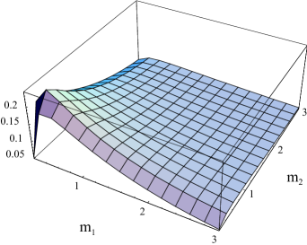
FIG. 1.: The value of $\delta x$ as a function of $m_{1}$ and $m_{2}$ in solar mass unit.

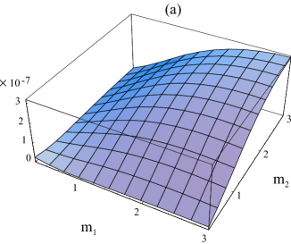
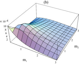
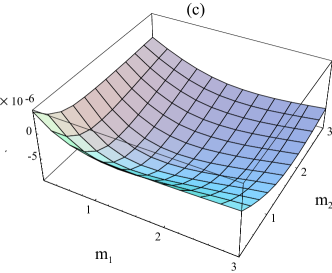
FIG. 2.: The values of (a)$g_{11}-1$, (b)$g_{22}-1$, (c)$g_{12}$, as functions of $m_{1}$ and $m_{2}$ in solar mass unit.

These facts suggest the usefulness of the new coordinates. First of all, the flatness of the metric allows us to use a uniform square grid to generate the template bank. Besides, there are several advantages. As long as we consider a small area in $\Gamma$, $x^{3},x^{4}$ and $x^{5}$ can be treated as constants. We can make use of this fact to develop an efficient algorithm to generate templates in frequency domain as we shall see in the succeeding subsection.

C An efficient algorithm to generate templates

We can express $\theta^{i}$ as linear functions of $x^{A}$ by solving Eq.(37) inversely. Thus, the phase function $\psi_{\theta}(f)$ is also a linear function of $x^{A}$. Since the effect of variation of $(x^{3},x^{4},x^{5})$ within a small area is negligibly small, the difference of the phase function

$$\Delta\psi(f)=\psi_{(X^{1}+\Delta X^{1},X^{2}+\Delta X^{2})}(f)-\psi_{(X^{1},X^{2})}(f)$$ (45)

is almost independent of $(X^{1},X^{2})$. Therefore, we can prepare the phase difference $e^{i\Delta\psi(f)}$ for various values of $(\Delta X^{1},\Delta X^{2})$ in advance. Then we can calculate the template $\tilde{h}_{(X^{1}+\Delta X^{1},X^{2}+\Delta X^{2})}(f)$ just by multiplying the corresponding phase difference by the template at $(X^{1},X^{2})$ as

$$\tilde{h}_{(X^{1}+\Delta X^{1},X^{2}+\Delta X^{2})}(f)=\tilde{h}_{(X^{1},X^{2})}(f)\,e^{i\Delta\psi(f)}.$$ (46)

Hence, once we calculate one template, we do not have to call subroutines of the sinusoidal functions to generate neighboring templates of it. Since the computation of sinusoidal functions is slow in many compiler, this algorithm significantly reduces the computation cost to generate templates.

Before closing this secton, we remark on the choice of the maximum frequency $f_{max}$. So far, we have been neglecting the fact that, in general, the maximum frequency $f_{max}$ depends on the template parameters. When we consider binaries with large mass, the frequency at the last stable circular orbit becomes lower than the maximum frequency which is determined by the shape of the noise power spectrum. Since our post-Newtonian templates are no longer valid beyond the last stable orbit, the maximum frequency should be chosen below the corresponding frequency. Even in that case, we think that our new coordinates are still useful by the following reason. The match determined with larger $f_{max}$ is likely to underestimate the correct value. Hence, the grid spacing determined by using our new coordinates tends to be closer than that determined by more accurate estimation. Therefore, to adopt constant $f_{max}$ in determining the template bank would be safe in the sense that it is less likely to miss detectable events. Although the number of templates increases with the choice of constant $f_{max}$, such effect is very small. This is because the number of templates with relatively large mass is not very large. Recall that the number of template are dominated by templates with small mass $m\sim m_{min}$[10].

III new fast algorithm for hierarchical search

If we try to search gravitational waves from coalescing binaries with mass $M\geq 0.2M_{\odot}$, we have to calculate the correlations $(\tilde{s}(f),\tilde{h}(f))$ for several$\times 10000$ templates with different mass parameters[10] . The computation cost to evaluate such a large number of correlations is very expensive. One promising idea to reduce the computation cost is the technique of hierarchical search. The basic idea of hierarchical search is as follows. At the first step, we examine the correlations with a smaller number of templates located more sparsely. In order not to lose the candidates of events, we set a sufficiently low threshold of the filtered signal-to-noise $\rho$ at the first step. If a set of parameters $(X^{1},X^{2},t_{c})$ is selected as a candidate, we examine the correlations between the data and the neighboring templates by using a finer mesh.

A simple scheme for two step search has been already discussed in Ref.[5]. However, there seems to be a problem in realizing the basic idea mentioned above. It has been pointed out that the distribution of the amplitude of the detector noise will not follow the simple stationary Gaussian statistics[11]. The non-stationary and non-Gaussian nature of the detector noise will produce a lot of events with large value of $\rho$. Namely, there seems to exist a non-Gaussian tail part in the distribution of $\rho$. In order to identify real events, we need to keep the expected number of fake events small by choosing the threshold of $\rho$ as being sufficiently large. Hence, the existence of the non-Gaussian tail requires a larger value of threshold of $\rho$. This leads to a significant loss of detector sensitivity. To avoid such a loss, it was proposed to use a $\chi^{2}$-test as a supplementary criterion.

Here, $\chi^{2}$ is defined as follows. First we divide each template into mutual independent $n$ pieces,

$$\tilde{h}_{(c,s)}(f)=\tilde{h}^{(1)}_{(c,s)}(f)+\tilde{h}^{(2)}_{(c,s)}(f)+\cdots+\tilde{h}^{(n)}_{(c,s)}(f),$$ (47)

and we calculate

$$z^{(i)}_{(c,s)}=(\tilde{s},\tilde{h}^{(i)}_{(c,s)}),\quad\bar{z}^{(i)}_{(c,s)}=\sigma_{(i)}^{2}\times(\tilde{s},\tilde{h}_{(c,s)}),$$ (48)

with

$$\sigma_{(i)}^{2}=(\tilde{h}^{(i)}_{(c)},\tilde{h}^{(i)}_{(c)})=(\tilde{h}^{(i)}_{(s)},\tilde{h}^{(i)}_{(s)}).$$ (49)

Then $\chi^{2}$ is defined by

$$\chi^{2}=\sum_{i=1}^{n}\left[{\left(z^{(i)}_{(c)}-{\bar{z}^{(i)}_{(c)}}\right)^{2}+\left(z^{(i)}_{(s)}-{\bar{z}^{(i)}_{(s)}}\right)^{2}\over\sigma_{(i)}^{2}}\right].$$ (50)

This quantity must satisfy the $\chi^{2}$-statistics with $2n-2$ degrees of freedom and must be independent of $\rho=\sqrt{z_{(c)}^{2}+z_{(s)}^{2}}$, as long as the detector noise is Gaussian. However, as reported in Ref. [11], events with large $\chi^{2}$ in reality occur more often than in the case of Gaussian noise. There is a strong tendency that events with large $\chi^{2}$ have a large value of $\rho$ on average. Thus, by changing the threshold of $\rho$ depending on the value of $\chi^{2}$, we can reduce the number of fake events without any significant loss of detector sensitivity. Hence, it will be necessary to implement the $\chi^{2}$-test even in the simple one step search case. However, if we try to evaluate $\chi^{2}$, the computation cost becomes more expensive. Thus, it is strongly desired to implement an efficient algorithm to reduce the computation cost.

Now, we discuss a method of two step hierarchical search taking into account the presence of non-Gaussian noise. At the first step search, a large number of candidates for the second step search with large $\rho$ value will appear due to the non-Gaussianity of noise. As is mentioned above, in order not to lose the detector sensitivity, it is desired to introduce the $\chi^{2}$-test, and to keep the threshold of $\rho$ small. Furthermore, by introducing the $\chi^{2}$-test at the first step, we can reduce the number of candidates for the second step search. Thus, the $\chi^{2}$-test is also effective to reduce the computation cost for the second step. However, the $\chi^{2}$-test at the first step increases the computation cost for the first step. This increase in the computation cost can be very large in the presence of non-Gaussian noise because the number of fake events which exceed the threshold of $\rho$ at the first step is much larger than that expected in the case of Gaussian noise. Then, we must compute a lot of $\chi^{2}$ values at the first step. When we take into account these effects, the advantage of the two step search, which is estimated to be about factor $30$ in comparison with the simple one step search in the case of Gaussian noise[5], will be significantly reduced or will be totally lost. Hence, in order to make use of the potential advantage of the two step search, we need other ideas to reduce the computation cost further. Here we present two new ideas of this kind.

(a)

$\to X^{1}$

$\begin{array}[]{c}X^{2}\\ \uparrow\end{array}$   0.0   0.5   1.0   1.5   2.0 2.0 0.774 0.760 0.757 0.746 0.717 1.5 0.828 0.800 0.777 0.765 0.733 1.0 0.889 0.857 0.804 0.771 0.733 0.5 0.947 0.918 0.821 0.742 0.682 0.0 1.000 0.914 0.765 0.644 0.592 -0.5 0.947 0.886 0.774 0.653 0.553 -1.0 0.889 0.865 0.791 0.692 0.589 -1.5 0.828 0.831 0.794 0.724 0.637 -2.0 0.774 0.787 0.777 0.737 0.674

(b)

$\begin{array}[]{c}X^{2}\\ \uparrow\end{array}$   0.0   0.5   1.0   1.5   2.0 2.0 0.781 0.759 0.770 0.747 0.735 1.5 0.838 0.817 0.797 0.766 0.739 1.0 0.904 0.873 0.812 0.764 0.710 0.5 0.961 0.907 0.809 0.728 0.673 0.0 0.984 0.911 0.791 0.663 0.608 -0.5 0.961 0.893 0.777 0.666 0.565 -1.0 0.904 0.869 0.803 0.699 0.598 -1.5 0.838 0.841 0.809 0.732 0.646 -2.0 0.781 0.803 0.787 0.750 0.681

TABLE 1. Tables of maximum correlations for various choices of $\Delta{\bf X}$ (a) with 5000Hz sampling and (b) with 1250Hz sampling.

The first one is very simple. At the first step search, we can reduce the sampling rate of the data. The low sampling rate results in the reduction in the filtered signal-to-noise mainly due to the mismatch in $t_{c}$. However such reduction can be compensated by a very small change of the threshold of $\rho$. In the case of the “TAMA noise curve”, we can allow the sampling rate as low as about 1000Hz. The values of match between two templates with various $\Delta{\bf X}$ are shown in Table.1(a), where we adopted 5000Hz as the sampling rate. The same quantities for 1250Hz sampling are shown in Table.1(b). Here, one of the templates is considered as a normalized signal without noise, and the other as a search template. The signal is normalized to satisfy $(h,h)=1$ with $f_{max}=2500Hz$ in both cases of Table.1(a) and Table.1(b). On the other hand, the search template is normalized with $f_{max}=2500Hz$ in the case of Table.1(a) and with $f_{max}=625Hz$ in the case of Table.1(b). We find that the difference of the values of match between these two cases are very small especially for large $|\Delta{\bf X}|$. Therefore, detection probability for a fixed threshold of $\rho$ is not significantly lost even if we adopt a rather small sampling rate at the first step search, at which we adopt a relatively large spacing for the template bank. The reduction in the sampling rate directly reduces the computation cost. The usual FFT routine requires effective floating point operations proportional to $\sim N\ln N$ to compute the Fourier transform of the data with length $N$. Furthermore, for most of FFT routines and computer environments, the effective FLOPS value for FFT is larger for smaller $N$. Thus, the reduction factor for the computation cost due to adopting a smaller FFT length is much larger than one expects naively.

The second idea is more important. What we need to evaluate is the correlation

$$Z=(\tilde{h},\tilde{s}) = \int_{-f_{max}}^{f_{max}}df{\tilde{h}_{\bf X}(f)\tilde{s}^{*}(f)\over S_{n}(f)}$$ (51)

$$\approx {\cal N}\Delta f\sum_{j=1}^{N}\left[{\tilde{s}^{*}(f_{j})e^{i\psi_{\bf X}(f_{j})}\over f_{j}^{7/6}S_{n}(f_{j})}\right]e^{2\pi if_{j}t_{c}}.$$ (52)

where we take it into account that in reality we deal with a discrete time sequence of data with length $N$. $\Delta f$ is given by the sampling rate divided by $N$, and $f_{j}:=\Delta f(j-N/2)$. The correlations for various values of $t_{c}$ are calculated simultaneously by taking the Fourier transform of the array defined by the quantity inside the square brackets in the last line of the above equation. This scheme is efficient enough when we do not have any guess about $t_{c}$. However, when we perform the second step search we have a good estimate of $t_{c}$ at which the maximum correlation is expected to be achieved. We denote it by $\hat{t}_{c}$. In this case, we need to evaluate $Z$ only for $t_{c}$ which are close to $\hat{t}_{c}$. Also for templates, we have a good guess for the mass parameters, $\hat{\bf X}$. Thus, we need to calculate the correlation $Z$ only for a cluster of the templates neighboring to $\hat{\bf X}$.

Once $\hat{t}_{c}$ and $\hat{\bf X}$ are specified, we can rewrite the above expression in a very suggestive form as

$$Z\approx{\cal N}\Delta f\sum_{k=1}^{N/m-1}\sum_{j=m(k-1/2)+1}^{m(k+1/2)}A_{j}\times B_{j},$$ (53)

with

$$A_{j} = {\tilde{s}^{*}(f_{j})e^{i\psi_{\hat{\bf X}}(f_{j})+2\pi if_{j}\hat{t}_{c}}\over f_{j}^{7/6}S_{n}(f_{j})},$$ (54)

$$B_{j} = e^{i\Delta\psi(f_{j})+2\pi if_{j}\Delta t_{c}}.$$ (55)

Here $\Delta\psi(f_{j}):=\psi_{\bf X}(f_{j})-\psi_{\hat{\bf X}}(f_{j})$ and $\Delta t_{c}:=t_{c}-\hat{t}_{c}$. We have also introduced $m$ as a certain integer which divides $N$. As long as both $|\bf X-\hat{\bf X}|$ and $|t_{c}-\hat{t}_{c}|$ are sufficiently small, the factor $B$ is a slowly changing function of frequency. Hence, unless $m$ is not large, $B$ can be moved outside the second summation in Eq.(53). Then, introducing

$$A^{\prime}_{k}=\sum_{j=m(k-1/2)+1}^{m(k+1/2)}A_{j},$$ (56)

we obtain

$$Z \approx {\cal N}\Delta f\sum_{k=1}^{N/m-1}A^{\prime}_{k}\times B_{mk}$$ (57)

$$= {\cal N}\Delta f\sum_{k=1}^{N/m-1}\left[A^{\prime}_{k}e^{i\Delta\psi(f_{mk})}\right]\times e^{2\pi if^{\prime}_{k}\Delta t_{c}},$$ (58)

where $f^{\prime}_{k}:=m\Delta f\left(k-{N\over 2m}\right)$. The expression in the last line can be evaluated by applying the FFT routine to the array defined by the quantity inside the square brackets. The correlation between two templates for various values of $\Delta{\bf X}$ and $\Delta t_{c}$ are calculated by using this method. The results are shown in Table.2 for $N/m=1024,2048$ and $4096$. We find that $N/m$ can be taken as small as $2048$ without significant loss in accuracy.

(a)

$~{}~{}\Delta t_{e}$(sec)	$~{}~{}m=4096~{}~{}$	$~{}~{}m=2048~{}~{}$	$~{}~{}m=1028~{}~{}$
0.0000	1.000	1.000	1.000
0.0128	1.000	0.999	0.994
0.0248	0.999	0.994	0.975

(b)

$~{}~{}\Delta t_{e}$(sec)	$~{}~{}m=4096~{}~{}$	$~{}~{}m=2048~{}~{}$	$~{}~{}m=1028~{}~{}$
0.0000	0.765	0.765	0.765
0.0128	0.764	0.763	0.760
0.0248	0.763	0.760	0.746

(c)

$~{}~{}\Delta t_{e}$(sec)	$~{}~{}m=4096~{}~{}$	$~{}~{}m=2048~{}~{}$	$~{}~{}m=1028~{}~{}$
0.0000	0.774	0.774	0.774
0.0128	0.774	0.773	0.769
0.0248	0.773	0.769	0.755

TABLE 2. Tables of maximum correlations for various choices of $m$ and $\Delta t_{e}=\hat{t}_{e}-t_{e}^{(c)}$ with (a) $\Delta{\bf X}=(0,0)$, (b)$\Delta{\bf X}=(1,0)$ and (c)$\Delta{\bf X}=(0,2)$.

Furthermore, as an advantage of our new coordinates, the factor $e^{i\Delta\psi(f_{mk})}$ can be well approximated by the one obtained by setting $\Delta x^{3}=\Delta x^{4}=\Delta x^{5}=0$. It means that this factor is almost independent of the values of $(X^{1},X^{2})$. Thus, we have to calculate this factor only once at the beginning of the second step search. Since the array $A^{\prime}_{k}$ is independent of $\Delta{\bf X}$, the quantity inside the square brackets in Eq. (58) for various values of $\Delta{\bf X}$ is simply given by $A^{\prime}_{k}$ times the pre-calculated factor $e^{i\Delta\psi(f_{mk})}$. This fact manifestly leads to an additional reduction in the computation cost.

The same technique can be used to evaluate $\chi^{2}$, i.e., $Z^{(i)}$, just by replacing the array $A^{\prime}_{k}$ with the same quantities multiplied by an appropriate window function.

IV conclusion

We discussed a method of analyzing data from interferometric gravitational wave detectors to detect gravitational waves from inspiraling compact binaries based on the technique of matched filtering. We described a brief sketch of several new techniques which would be useful in hierarchical search of gravitational waves.

First, we proposed new parameters which label templates of gravitational waves from inspiraling binaries. These new parameters are chosen so that the metric on the template space becomes almost constant. We found that the template space can be well approximated by two dimensional flat Euclidean metric. Thus, by using these parameters as coordinates for the template space, the problem of the template placement becomes very simple. Say, we can use a simple uniform square grid to specify the grid points for the bank of templates. Furthermore, we found that, by using new parameters, we can introduce an efficient method to generate templates in frequency domain. The reduction in the computation cost is achieved by using the property of our new coordinates that one template can be translated into another with different mass parameters by just multiplying pre-calculated coefficients to the original template. Therefore, we can generate a set of templates from one template avoiding calculation of the sinusoidal functions.

Next, we discussed a method of two step hierarchical search. Due to the non-stationary and non-Gaussian nature of the detector noise, we will have to introduce a $\chi^{2}$-test when we analyze real data. When we take into account this fact, it becomes very difficult to obtain large reduction in the computation cost by applying naive two-step hierarchical search strategy. To solve this difficulty, we proposed two new techniques to reduce the computation cost in the two step search. One is to use a lower sampling rate for the first step search. By using this technique, we can reduce the length of FFT by factor 2 or 4 keeping the loss of correlation within an acceptable level. The second technique, which is more important, makes use of the fact that a good guess for the coalescence time and the mass parameters has been obtained as a result of the first step search at the time when we perform the second step search. We found that the length of FFT for the second step search can be reduced down to about 2048.

Based on the new techniques discussed in this paper, we have developed a hierarchical search code to analyze data from the TAMA300 detector. The details of this code and the result of the analysis of the first TAMA300 data will be presented elsewhere.

- [1] For recent development of the laser interferometers, and the details of the data taking of TAMA300 in 1999, see ”Gravitational Wave Detection”, Proceedings of the 2nd TAMA workshop, (Universal Academy Press, Tokyo), in press.
- [2] C. Alcock et al., Astrophys. J. 486, 697 (1997).
- [3] T. Nakamura, M. Sasaki, T. Tanaka, and K.S. Thorne, Astrophys. J. Lett. 487, L139 (1997); K. Ioka, T. Chiba, T. Tanaka, and T. Nakamura, Phys. Rev. D58, 063003, (1998); K. Ioka, T. Tanaka, and T. Nakamura, Phys. Rev. D60, 083512, (1999).
- [4] B.J. Owen, Phys. Rev. D53, 6749 (1996).
- [5] S.D. Mohanty and S.V. Dhurandhar, Phys. Rev. D54, 7108 (1996); S.D. Mohanty Phys. Rev. D57, 630 (1998).
- [6] This is an analytic fit to the TAMA phase II sensitivity provided to us by D.Tatsumi and N.Kanda (private communication).
- [7] L. Blanchet, T. Damour, B. Iyer, C.M. Will, and A.G. Wiseman, Phys. Rev. Lett. 74, 3515 (1995).
- [8] S. Droz, D.J. Knapp, E. Poisson, and B.J. Owen, Phys. Rev. D59, 124016 (1999).
- [9] C. Cutler and E.E. Flanagan, Phys. Rev. D49, 2658 (1994).
- [10] B.J. Owen and B. S. Sathyaprakash, Phys.Rev. D60, 022002 (1999).
- [11] B. Allen et al. Phys. Rev. Lett. 83, 1498 (1999).
- [12] H. Tagoshi and T. Tanaka, in preparation.
- [13] B. Allen et al. GRASP software package, http://www.lsc-group.phys.uwm.edu/ ballen/grasp-distribution/ .