Exact symmetric cosmologies with local Mixmaster dynamics††thanks: e-mail: berger@oakland.edu, vincent.moncrief@yale.edu
Abstract
By applying a standard solution generating technique, we transform an arbitrary vacuum Mixmaster solution on to a new solution which is spatially inhomogeneous. We thereby obtain a family of exact, spatially inhomogeneous, vacuum spacetimes which exhibit Belinskii, Khalatnikov, and Lifshitz (BKL) oscillatory behavior. The solutions are constructed explicitly by performing the transformations on numerically generated, homogeneous Mixmaster solutions. Their behavior is found to be qualitatively like that seen in previous numerical simulations of generic symmetric cosmological spacetimes on .
98.80.Dr, 04.20.J
I Introduction
Recent numerical studies [1] have provided strong evidence that -symmetric, vacuum spacetimes on generically develop Mixmaster-like, oscillatory singularities of the type predicted long ago by Belinskii, Khalatnikov and Lifschitz (BKL) [2, 3, 4, 5, 6]. These results confirm numerically some of the most surprising features of the BKL prediction, namely that nearby spatial points are effectively decoupled in their asymptotic metric evolution and that the metric variables at each of these points evolve, at least qualitatively, like those of a Mixmaster spacetime.
Several years ago B. Grubišić and one of us (V.M.) [7] made an analytical effort to generate some exact vacuum spacetimes which were spatially inhomogeneous and which were expected to exhibit the sort of oscillatory singularities which have since been seen in the numerical studies [1]. That effort was not completed at the time since it was not realized that several seemingly intractable integrals actually cancel in the course of the calculations leaving only elementary computations to be done. We shall therefore complete that project here and use the results to compare, in a more quantitative way, the numerical results with some exact oscillatory singularities.
To generate new solutions having Mixmaster-like oscillations, we begin with the actual Mixmaster solutions and apply a standard solution generating technique. We choose one of the Killing fields shared by the Mixmaster family and treat it as the generator of a spacelike action on , ignoring the presence of the other Killing symmetries. We compute the twist potential associated with the chosen Killing field and reexpress the field equations, in a well-known way [8], as a Kaluza-Klein reduced system on the base manifold of the -bundle . The field equations on the base take the form of Einstein gravity coupled to a wave map whose target space is the hyperbolic plane, . The isometry group of this latter space, , acts on the base fields in a natural way so as to transform the given solution to a family of potentially inequivalent solutions.
By a careful choice of the applied group element one can arrange that the transformed solution either lifts to the same bundle defined for the original spacetime or perhaps to a different one (e.g., the trivial bundle,, or a “squashed sphere”, ). Typically, the new solutions will preserve only the Killing field that generates the common action and not preserve those Killing fields of the seed solutions which fail to commute with the chosen generator. Thus the new solutions are expected to be spatially inhomogeneous and yet to exhibit Mixmaster-like oscillations inasmuch as their metrics are parametrized by the same functions appearing in the Mixmaster seed metrics themselves.
A previous application of this technique involved transforming an infinite dimensional family of “generalized Taub-NUT” spacetimes defined on , which have smooth Cauchy horizons at their “singular” boundaries, to a new family of curvature singular spacetimes defined on [9]. Because of the special nature of the seed solutions in this case, the transformed solutions developed only velocity dominated singularities and never exhibited Mixmaster-like oscillations. A new technique based upon expressing the Einstein evolution equations in a so-called Fuchsian form seems capable of significantly enlarging this set of rigorous, -symmetric, curvature singular cosmological spacetimes but, so far, is also only capable of yielding velocity dominated singularities [10, 11]. So far as we know the solutions presented for the first time here are the only known exact inhomogeneous vacuum spacetimes which exhibit Mixmaster oscillations. Though only a finite dimensional family they presumably display behavior representative of more general, -symmetric vacuum spacetimes and thus warrant comparison with numerically produced -solutions. Making such a comparison is the second main aim, after producing the solutions themselves, of this paper. As a byproduct of this work, we also resolve a potential paradox that was pointed out in Ref. [7]. There it was shown that every -symmetric vacuum spacetime admits a certain gauge invariant conserved quantity which is expressible purely locally in terms of the instantaneous Cauchy data for that solution and serves as a Casimir invariant for the action. For generic solutions this quantity is known to be non-trivial but, if non-trivial for the Mixmaster subfamily, would seem to contradict the anticipated “chaos” of the Mixmaster dynamics [12, 13, 14]. The only sensible resolution, as was discussed in Ref. [7], is that the quantity actually vanishes on the Mixmaster subfamily. This we find to be the case by explicit calculation.
The inhomogeneity in our transformed solutions is produced, roughly speaking, by the fact that we choose to reduce with respect to a Killing field which fails to commute with the remaining Killing fields of the seed metric. This is unavoidable with the generic Mixmaster solution but special cases such as the Taub-NUT metrics allow for different possibilities. The additional Killing field admitted by Taub space commutes with all the generators and is preserved upon reduction with respect to one of these (non-abelian) generators. The resulting spacetime has therefore (at least) two commuting Killing fields and is thus a special case of the so-called Gowdy family of spacetimes. By contrast one could instead choose to reduce with respect to the additional, commutative Killling field but, in this case, all the symmetries are preserved and one arrives, as was first shown by Geroch [15], at only the Kantowski-Sachs (i.,e. locally interior Schwarzschild) spacetime.
One might wonder if the “new” solutions we produce are really inhomogeneous at all or perhaps because of their expression in an unusual gauge, are merely homogeneous solutions in disguise. We shall use the Gowdy transform of Taub space mentioned above, to show that this is not the case—the new solutions are not in general globally homogeneous.
II Mixmaster spacetimes
The Mixmaster spacetimes are spatially homogeneous vacuum metrics on whose line elements can be written
| (1) |
Here the are a global, analytic basis of one-forms on expressible in terms of the usual Euler angle coordinates by
| (2) | |||||
| (3) | |||||
| (4) |
These forms, and therefore the above line element, are invariant with respect to the action on generated by the Killing field whose orbits yield a Hopf fibration of , i.e. make into a principal fiber bundle over with bundle projection given by
| (5) |
Of course the Mixmaster metrics are invariant with respect to a full action generated by Killing fields
| (6) | |||||
| (7) | |||||
| (8) |
but, for the transformations we shall consider, only invariance with respect to will in general be preserved.
The equations of motion for the Mixmaster solutions are most simply expressed in a gauge for which where they take the form
| (9) | |||||
| (10) | |||||
| (11) |
and are to be supplemented by the Hamiltonian constraint
| (12) | |||
| (13) |
In terms of the Misner anistropy variables ,
| (14) | |||||
| (15) | |||||
| (16) |
and the chosen gauge condition is . We now rewrite the line element in the -symmetric form developed in Refs. [8] and [16]. Taking and noting that the shift vector vanishes we express in the form
| (17) | |||
| (18) |
where is the scalar field given explicitly by
| (20) | |||||
Since is invariant with respect to the action generated by it induces a function on the quotient manifold which (with a slight abuse of notation) we shall also designate by . In a similar way one finds induced upon the quotient manifold a Lorentzian metric
| (21) |
and a one-form field
| (22) |
where . These forms are slightly specialized because of the vanishing of the shift vector field in . The most general -symmetric line element would yield
| (23) | |||||
| (24) |
The explicit formulas for the Lorentzian metric and the one-form potential may be read off upon expressing in the form of Eq. (1). One finds that
| (25) | |||||
| (27) | |||||
| (28) | |||||
| (29) | |||||
| (30) | |||||
| (31) |
and computes, for example, that
| (32) |
As in Refs. [8] and [16] we introduce the momenta conjugate to , which, taken together, parameterize the full spatial metric and its conjugate momentum . For the case of vanishing shift the formulas relating the momentum variables to the metric variables are given by
| (33) | |||||
| (34) | |||||
| (35) |
For the Mixmaster metrics one computes that
| (36) | |||
| (37) | |||
| (38) |
These momenta (along with which we shall not need explicitly) project to yield smooth tensor densities on the base manifold and one easily verifies that which is one of the components of the momentum constraint.
Note that the connection one-form on given by
| (39) |
does not project to yield a one-form on the base but that the difference between this connection one form and the reference one form does yield a one-form (namely ) which projects to the base. Even though itself does not project to the base, its exterior derivative (i.e., the curvature of the connection ) does project. Pulling back the induced two-form to a = constant slice of the base manifold and computing its dual, one gets a scalar density defined by
| (40) | |||||
| (41) |
whose explicit form is
| (43) | |||||
One computes on an arbitrary constant slice of the base manifold, that
| (44) |
The value reflects the particular bundle under study and would be the same for any -symmeteric metric defined on this bundle.
Taking into account the equation satisfied by and the fact that admits no non-trivial harmonic one forms, we now introduce the “twist potential” function (a salar field on ) by imposing
| (45) | |||||
| (46) |
These equations are self consistent and yield the solution
| (48) | |||||
which is unique up to the additive constant where is the function defined by
| (49) |
As discussed in Refs. [8] and [16] the fields induced upon the base manifold satisfy a dimensional system of Einstein-wave map equations for which the target space of the wave map is hyperbolic two-space (endowed with global coordinates and the natural metric ). As a consequence of the isometry group of this target space the Einstein-wave map system admits three independent constants of the motion which serve as the Hamiltonian generators of the action of on the phase space of fields . These conserved quantities are given explicitly by the integrals
| (50) | |||||
| (51) | |||||
| (52) |
and we have already noticed that for the Mixmaster spacetimes in particular. In fact would take this same value for any -symmetric vacuum metric on but for other bundles over the same base the value would (as discussed in Refs. [8] and [16]) be modified to where is an integer determining the Chern class of the bundle. In particular, for solutions on the trivial bundle , would vanish whereas if the bundle would correspond to various “squashed spheres” rather that a true .
Note that, in view of the integral expression for arising in the formula for , both and are non-local in time. The same feature occurs in more general symmetric solutions but this non-locality cancels from the Casimir invariant
| (53) |
which, however, vanishes identically for the Mixmaster family of solutions (though not in general). The vanishing of resolves a potential mystery pointed out in Ref. [7] whereby a non-vanishing, local, constant of the motion for Mixmaster metrics would seem to contradict their empirically observed “chaotic” properties.
More specifically one finds, for the Mixmaster metrics, that
| (54) | |||||
| (55) | |||||
| (56) |
so that . The non-locality of and sidesteps any conflict with the observed “chaos” in Mixmaster solutions since, in fact, any Hamiltonian system will admit such non-local constants of the motion. To see this (even for a chaotic system) simply time integrate Hamilton’s equations and express the initial values of the canonical variables in terms of time integrals of their driving “forces.”
III The new solutions
To generate new solutions of Einstein’s equations from a given one (such as a Mixmaster solution) we choose an element ,
| (57) |
and transform the fields according to
| (58) | |||||
| (59) | |||||
| (60) | |||||
| (61) |
while leaving invariant. The induced transformation of the conserved quantities (by the so-called co-adjoint action of )is found to be [9]
| (62) | |||||
| (63) | |||||
| (64) | |||||
| (65) |
To avoid a trivial transformation we shall require that be non-zero and, to ensure that the transformed solution lifts to an bundle over, we shall demand that
| (66) |
Defining
| (67) |
we see from Eq. (57) that
| (68) | |||||
| (69) | |||||
| (70) |
Setting gives the restriction
| (71) |
or, equivalently,
| (72) |
which can always be solved for since .
Exploiting the fact that , hence also , is conserved one finds that the integral occurring in the formula for can be expressed as
| (73) |
(this is also easily verified upon differentiation by using the equations of motion (9)). Using this result, one can easily show that
| (74) | |||
| (75) | |||
| (76) |
With this and Eq. (20) for one easily evaluates the transformed field variables using Eq. (58). The new spacetime metric thus takes the form
| (78) | |||||
where however, remains to be computed. As discussed in Ref. [8], can be expanded (via the Hodge decomposition for a one-form on ) as
| (79) |
where and and are suitable functions defined on . The equation for is
| (80) |
which, upon substitution of the decomposition (79), becomes
| (81) |
a Poisson equation for for which the necessary and sufficient integrability condition is ensured by Eq. (66). This uniquely determines , at fixed , up to an arbitrary additive constant and leaves arbitrary. The presence of reflects the freedom to make an arbitrary coordinate transformation of the form without affecting the -form of the spacetime metric.
The time development of can now be obtained by integrating the (zero shift) evolution equation
| (82) | |||||
| (83) |
with determined as above.
Equations (80) and (82) are consistent with each other by virtue of the Hamilton equations satisfied by . Note that whereas we have used the actual metric in defining a Hodge decomposition of , any smooth metric on could have been used instead. Furthermore one could have used Eq. (81) to determine at an arbitrary time and then adjusted the time dependence of to impose the zero shift condition which is implicit in Eq. (82). In either case the new metric (78) will satisfy the vacuum field equations on the chosen bundle over .
One might still wonder how we know that the transformed solutions are genuinely inhomogeneous. Could they not be merely homogeneous solutions disguised through the choice of a time slicing that is not adapted to the (hypothetical) homogeneity? To show that this is not the case, in general,we shall examine a special case for which the transformed solution has a hypersurface of time symmetry at , i.e., has . To arrange this, we choose the seed solution to have this property and make a careful choice of transformation parameters so that the desired feature is not destroyed by the transformation. We then show that the transformed spatial metric is not homogeneous as it would have to be for the resulting spacetime to have this property. The key point here is the fact that on any compact slice, having constant mean curvature the first and second fundamental forms would both have to be homogeneous in order that the spacetime have this property.
Consider a Mixmaster solution for which . This spacetime has the slice as a surface of time symmetry and, because of the Hamiltonian constraint, must satisfy
| (84) | |||
| (85) |
To maintain this property we choose the trivial target bundle by taking . We further simplify the computations by choosing and and find that the transformed metric at satisfies
| (86) | |||||
| (87) | |||||
| (88) | |||||
| (89) | |||||
| (90) |
Thus the new spatial metric induced at on is
| (93) | |||||
A straightforward computation of (the square of the Ricci tensor of this metric) proves that the resulting spacetime is not homogeneous. Indeed, the only vacuum homogeneous solution on is known to be the Kantowski-Sachs universe which does not have a hypersurface of time symmetry. It is possible to get the Kantowski-Sachs metric upon transformation of a Taub metric (i.e., a Mixmaster solution having ) but to do so one must reduce with respect to the “extra” Killing field the Taub metric possesses, , rather than with respect to the common Killing field of the Mixmaster family as we have done. The extra Killing field commutes with all the Killing symmetries of the Taub solution and allows all of these symmetries to be preserved upon reduction [15].
The Taub metric used in the example above, is known explicitly but exhibits no type oscillations. To see such oscillations in an inhomogeneous setting, we combine a previously developed code for solving the Mixmaster equations of motion with the transformations discussed above. Our results are discussed in the following section and compared with results derived from a general -syummetric, vacuum Einstein code.
IV Numerical results
Elsewhere we have shown that even the homogeneous Mixmaster model reproduces the local behavior seen in generic -symmetric cosmologies [17]. From Eq. (20), it is clear that is dominated by the largest of the Mixmaster scale factors , , or . The local oscillations seen in in the -symmetric models are interpreted as follows: Assume that the BKL approximate description of a homogeneous Mixmaster model as a sequence of Kasner epochs is valid. In a given approximate Kasner epoch assume and that is increasing. Then for while and are less than zero. The usual Mixmaster bounce changes the sign of and thus of . However, after the bounce, either (within an era) or (at the end of an era) becomes positive. When the growing scale factor surpasses the decreasing , will start to grow again since it will now track the new dominant scale factor. A similar analysis indicates that the remaining “dynamical” variables, , , and , depend on an order unity ratio of scale factors and thus do not oscillate, as does, between order unity and exponentially small values. (Here we shall use “order unity” to mean some finite value which is not exponentially small.)
In our previous numerical simulations of generic -symmetric cosmologies on , we noted that the oscillations in could be interpreted as bounces off the potentials and . For a Mixmaster solution, is exponentially small unless is of order unity while is exponentially small unless the two largest scale factors are approximately equal to each other [17]. This is clearly consistent with a presumption that the generic models exhibit local Mixmaster dynamics.
To explore the nature of the new inhomogeneous -symmetric models, we note that the transformed variables , , and will remain of order unity (i.e. they will not oscillate between exponentially small and order unity values) because the right hand sides of Eqs. (58b)-(58d) are always of order unity. On the other hand, is dominated by the behavior of the oscillatory since the denominator on the right hand side of Eq. (58a) is always order unity while the numerator oscillates.
To explore the differences between our new solution and the Mixmaster seed solution, we construct the new solutions as follows: First use the algorithm of Berger et al [18] to obtain a numericallly generated Mixmaster model. This code is known to solve the Mixmaster ODE’s with machine-level precision and can follow hundreds of bounces. The presumed stochastic properties of such a model imply that almost any Mixmaster initial conditions will yield generic Mixmaster behavior. Thus, we need only consider a single Mixmaster trajectory. Next, Eqs. (20), (36), (43), (48), (49), (67), and (73) are used to numerically evaluate , , , and from the numerically generated sequence of values of the BKL scale factors and their time derivatives. Finally, for a representative choice of the parameters and, e.g., , the transformed variables , , , and are computed using Eqs. (58).
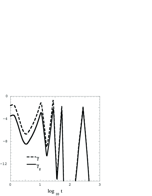
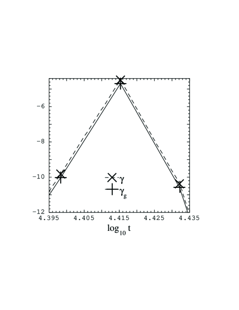
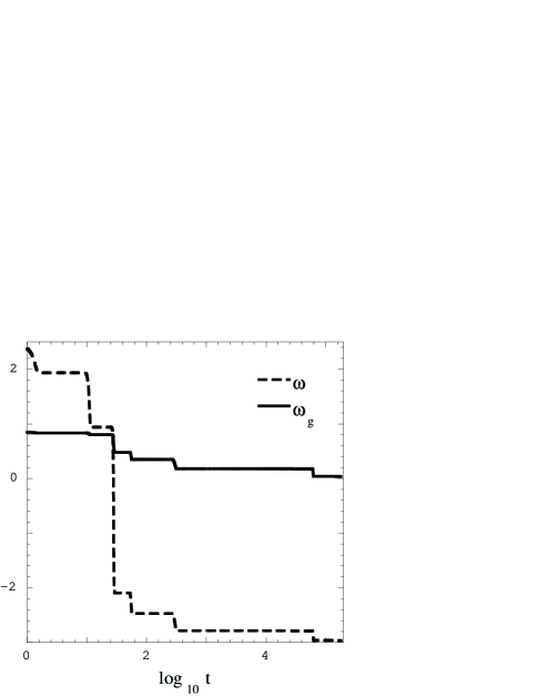
In Figures 1–3, we compare the Mixmaster and transformed and at a representative spatial point for typical Mixmaster seed and set of parameters. Note that, in Fig. 1, the original and transformed ’s become indistinguishable after only a small number of Mixmaster epochs. It is clear that this will be so from Eq. (20) for and Eq. (58a) for the transformation. Since and are found from the logarithm of Eqs. (20) and (58a), both and will be approximately equal to the logarithm of the largest scale factor and depend only logarithmically on the spatially dependent function associated with it. On a finer scale, in Fig. 2, the difference between the solutions (especially near the “bounce” where ) may be seen. On the other hand, as is seen in Fig. 3, and are always of order unity and may easily be distinguished.
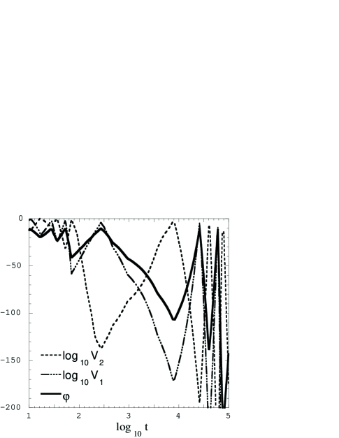
Figure 4 demonstrates the close link between Mixmaster dynamics and the oscillatory behavior observed in our studies of generic -symmetric models and should be compared to Figs. 2–6 in [1]. It shows the oscillations of (or essentially equivalently ), , and at a representative spatial point—reproducing the behavior seen in our simulations of generic -symmetric cosmologies. Since we know that these oscillations indicate local Mixmaster behavior in the new solutions, we can infer that the observed oscillations in the generic models also indicate local Mixmaster dynamics.
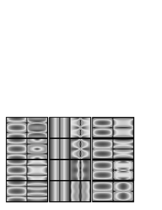
Since is the key variable in the -symmetric models and , one may then ask where these new -symmetric models differ from both Mixmaster and generic -symmetric models. First, we emphasize that, except at special values of the spatial coordinate angles, there are no qualitative differences attributable to spatial topology. The Mixmaster spatial dependence of course represents a realization of the Bianchi type IX symmetry. From Eq. (20), it is clear that three distinct spatial patterns will appear in (in the logarithm) depending on which scale factor dominates. In Fig. 5, we compare the spatial dependence of and for 12 epochs of the seed Mixmaster solution. The epochs are arranged according to the dominant scale factor. The numerical scale in each frame is chosen so that the average value of or is the centroid. (If this were not done, no spatial dependence would be visible.) From Eqs. (20) and (48), and have three possible spatial dependences. The transformation of Eqs. (58) clearly mixes the spatial dependence of and to form and . In Fig. 5, we see the evolving spatial dependence of . This is additional evidence that the new solutions are spatially inhomogeneous.
In generic -symmetric models, one could qualitatively interpret the asymptotic approach to the singularity as the evolution of a different Mixmaster model at every spatial point. In particular, the Mixmaster epochs have spatially dependent durations—bounces at different spatial points occur at different times. In contrast, our new solution is characterized as is Mixmaster itself by spatially independent epoch durations since the new solution bounces only when the seed solution does so. While one could modify the spacetime slicing to yield spatially dependent epoch durations, one would expect to be able to detect the difference between between a single underlying Mixmaster seed in the new solutions and a continuum of approximate Mixmaster solutions in the generic case.
Acknowledgments
We would like to thank the Institute for Theoretical Physics at the University of California / Santa Barbara for hospitality. BKB would like to thank the Institute for Geophysics and Planetary Physics of Lawrence Livermore National Laboratory for hospitality. This work was supported in part by National Science Foundation Grants PHY9732629, PHY9800103, PHY9973666, and PHY9407194.
Figure Captions
Figure 1. Comparison of and at a typical spatial point. The Mixmaster seed solution has initial values , , , , , and the Hamiltonian constraint (12) solved for . The parameters are , , , and .
Figure 2. Detail of the comparison of and . To emphasize the approach of to , data from later in the simulation of Fig. 1 are shown. The actual, saved data values are indicated by the and symbols.
Figure 3. Comparison of and for the same models as in Fig. 1. Note that appears to decrease to zero. This is due to the fact that choice of parameters causes if .
Figure 4. New solution as an inhomogeneous -symmetric cosmology. As in previous studies of generic -symmetric cosmologies, , , and are shown at a typical spatial point.
Figure 5. Evidence for the spatial inhomogeneity of the new solutions. The spatial dependence of and is shown for the plane in a series of side-by-side frames arranged in three separate panels. Each pair of frames shows the spatial dependence of and respectively during an approximate Kasner epoch of the seed Mixmaster solution. The panels are grouped according to the identity of the dominant scale factor in the spatially homogeneous solution rather than sequentially. According to Eq. (20), will have the spatial dependence , , or depending on whether , , or respectively is dominant. In each of the three panels, the 4 left-hand frames reproduce one of these three spatial dependences with, reading from left to right, , , or dominant. In each case, the accompanying right-hand frame represents the spatial dependence of the corresponding for that epoch. In every case, the numerical scales for and have been centered on their average values to enhance the visibility of the spatial dependence.
REFERENCES
- [1] Berger, B. K. and Moncrief, V., Phys. Rev. D 58, 064023 (1998).
- [2] Belinskii, V. A. and Khalatnikov, I. M., Sov. Phys. JETP 30, 1174 (1969).
- [3] Belinskii, V. A. and Khalatnikov, I. M., Sov. Phys. JETP 29, 911 (1969).
- [4] Belinskii, V. A. and Khalatnikov, I. M., Sov. Phys. JETP 32, 169 (1971).
- [5] Belinskii, V. A., Lifshitz, E. M., and Khalatnikov, I. M., Sov. Phys. Usp. 13, 745 (1971).
- [6] Belinskii, V. A., Khalatnikov, I. M., and Lifshitz, E. M., Adv. Phys. 31, 639 (1982).
- [7] Grubis̆ić, B. and Moncrief, V., Phys. Rev. D 49, 2792 (1994).
- [8] V. Moncrief, Ann. Phys. (N.Y.) 167, 118 (1986).
- [9] V. Moncrief, Class. Quantum Grav. 4, 1555 (1987).
- [10] S. Kichenassamy and A.D. Rendall, Class. Quantum Grav. 15, 1339 (1998).
- [11] J. Isenberg and V. Moncrief, unpublished.
- [12] C. W. Misner, Phys. Rev. Lett. 22, 1071 (1969).
- [13] J.D. Barrow, Phys. Rep. 85, 97 (1982).
- [14] , N.J. Cornish and J. Levin, Phys. Rev. Lett. 78, 998 (1997).
- [15] R. Geroch, J. Math. Phys. 12, 918 (1971).
- [16] V. Moncrief, Class. Quantum Grav. 7, 329 (1990).
- [17] B.K. Berger and V. Moncrief, unpublished.
- [18] Berger, B. K., Garfinkle, D., and Strasser, E., Class. Quantum Grav. 14, L29 (1996).