Stability of self-gravitating magnetic monopoles

Abstract

The stability of a spherically symmetric self-gravitating magnetic monopole is examined in the thin wall approximation: modeling the interior false vacuum as a region of de Sitter space; the exterior as an asymptotically flat region of the Reissner-Nordström geometry; and the boundary separating the two as a charged domain wall. There remains only to determine how the wall gets embedded in these two geometries. In this approximation, the ratio $k$ of the false vacuum to surface energy densities is a measure of the symmetry breaking scale $\eta$. Solutions are characterized by this ratio, the charge on the wall $Q$, and the value of the conserved total energy $M$. We find that for each fixed $k$ and $Q$ up to some critical value, there exists a unique globally static solution, with $M\simeq Q^{3/2}$; any stable radial excitation has $M$ bounded above by $Q$, the value assumed in an extremal Reissner-Nordström geometry and these are the only solutions with $M<Q$. As $M$ is raised above $Q$ a black hole forms in the exterior: (i) for low $Q$ or $k$, the wall is crushed; (ii) for higher values, it oscillates inside the black hole. If the mass is not too high these ‘collapsing’ solutions co-exist with an inflating bounce; (iii) for $k$, $Q$ or $M$ outside the above regimes, there is a unique inflating solution. In case (i) the course of the bounce lies within a single asymptotically flat region (AFR) and it resembles closely the bounce exhibited by a false vacuum bubble (with $Q=0$). In cases (ii) and (iii) the course of the bounce spans two consecutive AFRs. However, from the point of view of either region it resembles a monotonic false vacuum bubble.

I Introduction

Several years ago, Linde and Vilenkin pointed out the possibility that the core of a localized topological defect could inflate under appropriate conditions in a process that was aptly dubbed topological inflation [1, 2]. See also [3].

A common characteristic of such defects is some non-linear scalar field (the Higgs field) forced up in its core into a constant excited false vacuum state, falling through a transition layer to the true vacuum value remote from the core.

Without further refinement, a configuration of this type will always collapse, with or without gravity. The dynamics of this basic configuration, a so called false vacuum bubble, was studied in detail in the eighties by various groups, perhaps most comprehensively by Blau, Guendelman and Guth (BGG) in Ref.[4] where references to the earlier literature are provided. Their work was motivated, like Linde and Vilenkin’s, by the possibility that a false vacuum bubble could provide a seed for an inflationary universe [5].

They discovered that the essential radial dynamics of the scalar field is captured extremely accurately by a simple one dimensional mechanical caricature of the field configuration. This led them to consider the dynamics of a spherically symmetric region of false vacuum which is separated by a domain wall from an infinite true vacuum exterior (with zero energy density).

The energy momentum tensor of false vacuum is inherently homogeneous and isotropic. The Birkhoff theorem then constrains the spacetime it occupies to coincide with some patch of de Sitter space; the exterior is simply the Schwarzschild geometry truncated at the false vacuum boundary. In this model, it becomes clear that collapse does not necessarily spell the demise of the false vacuum interior. When gravity is taken into account, there are (at least) two spherically symmetric configurations associated with each sufficiently low value of conserved Arnowitt-Deser-Misner (ADM) mass $M$. While the smaller of the two, no matter what its initial radius, will always collapse to a vanishing radius, the other will inflate; but unexpectedly from an euclidean perspective, not at the expense of the exterior. This peculiar state of affairs is possible because the expansion occurs behind a minimal surface (a wormhole) in the Schwarzschild geometry connecting the false vacuum core to the exterior. While false vacuum is destroyed by the motion of the boundary, it is created exponentially faster in the interior. The wormhole itself, however, always collapses into a black hole.

Field theories admitting static configurations when gravity is turned on were first constructed in the eighties. Self-gravitating global monopoles were considered by Barriola and Vilenkin [6] (with additional insight provided in Ref. [7]). Gauge monopoles were considered by Gibbons [8], with the subsequent numerical solution of the static Einstein-Yang-Mills-Higgs equations by Ortiz [9] and Breitenlohner, Forgacs and Maison [10]. However, as Gibbons himself realized the balance of forces is not always possible when gravity is acting. As Linde and Vilenkin were later to show, if the symmetry-breaking scale is increased towards the Planck scale, at some point the interior radius will exceed the corresponding cosmological horizon, triggering the inflation of the interior. A bound exists beyond which static configurations necessarily become unstable. This process was studied by Sakai et al. [11, 12] by numerically solving the dynamical Einstein-Higgs and Einstein-Yang-Mills Higgs equations. The inflating core was not unlike an inflating false vacuum bubble. In Ref.[13] two of us showed how the model of a false vacuum bubble could be adapted to imitate the dynamics of a self-gravitating global monopole under these extreme conditions. Technically this was simple, involving the substitution of the Barriola-Vilenkin geometry describing the asymptotics of a global monopole for the exterior Schwarzschild geometry of the former. It was possible to capture, remarkably faithfully, the essential underlying physics of topological inflation found earlier by Sakai et al. The onset of topological inflation was very clearly indicated at $8\pi\eta^{2}=1$ (in natural units).

The details of topological inflation in a gauge monopole are very different. Here, the only long range field is the magnetic Coulomb field and the total energy is finite. However, the source resides on the core boundary which suggests the same mechanical caricature: de Sitter space inside, a domain wall, but with the Reissner-Nordström geometry outside. The structure of this geometry is very different from Schwarzschild. If the conserved charge to mass ratio of the configuration $Q/M\leq 1$, the analyically continued geometry possesses horizons, otherwise it contains a naked singularity. In this paper, we examine the above model in detail. Though simple in principle, a thorough analysis of the three-dimensional parameter space $(\eta$, $Q$, $M$) is complicated in practice. We will focus on the identification of the regimes of parameter space admitting solutions which are either static, collapsing or inflating within the core and we will examine the fate of these solutions as the relevant boundaries in parameter space are crossed.

Our results can be summarized as follows:

1. Fix $\eta$: for each non-vanishing value of $Q$ up to some critical value $Q_{0}$ there exists a unique stable and globally static configuration with a fixed core radius (a monopole) with mass $M_{0}\sim Q(Q/Q_{0})^{1/2}$. Stable radial oscillations of this configuration exist for all $M<Q$ above $M_{0}$. These are the only solutions with $M<Q$.

   Now raise $M$ above $Q$ but below some value $M_{+}$:

2. (i) For non-vanishing values of $Q$ up to some value $Q_{+}$ lower than $Q_{0}$, this radially oscillating solution falls through an event horizon and is terminated by the collapse of the exterior into a Reissner-Nordström black hole; (ii) for higher (but bounded) values of $Q$ radial oscillations lie within the inner horizon and get isolated by the collapse of the exterior (a monopole inside a black-hole); an inflating bounce co-exists with these solutions; (iii) if $Q$ or $M$ lies outside these two regimes, but $M$ lying above some minimum value, there is a unique inflating bounce.

3. The bounce occuring in these three regimes can be characterized roughly as follows: (i) the course of the bounce lies within a single asymptotically flat region (AFR) and it resembles closely the bounce exhibited by a false vacuum bubble (with $Q=0$); (ii),(iii) the course of the bounce spans two consecutive AFRs. However, from the point of view of either region it resembles a monotonic false vacuum bubble; In all cases, the expansion takes place behind an event horizon. These configurations are analogues in this model of the topologically inflating solutions observed numerically by Sakai [12] for large $\eta$.

4. All collapsing and monotonic solutions are ruled out as either unphysical or inconsistent with asymptotically flat boundary conditions.

Aspects of the model have been examined before. Indeed in the sixties, it received its first incarnation in Dirac’s proposal (without spin!) of a model of the electron as a closed charged conducting membrane surrounding a vacuum interior[14].

Tachizawa, Maeda and Torii focused on the stability of the monopole from the point of view of catastrophe theory [15], modeling the monopole core and exterior as we do but without an intermediate surface layer, a model originally proposed by Lee, Nair and Weinberg, in Ref. [16]. In this limit, the core radius exceeds the cosmological horizon when $\eta\sim 0.33$, signaling inflation. However, without the domain wall to transmit energy from the false vacuum, all dynamical possibilities are not faithfully represented. More recently, Alberghi, Lowe and Trodden [17] considered the model within the context of the Anti- de Sitter space/conformal field theory correspondence. For this purpose they catalogued accurately the possible trajectories of the charged false vacuum bubble. However, they did not consider how these trajectories depend on the values of $Q$, $M$ or $\eta$ and they did not consider the parameter regime $M<Q$ corresponding to stable configurations.

The paper is organized as follows. In Sec. II we introduce the model. In Sec. III, we determine all possible trajectories of the wall radius consistent with set values of $Q$, $\eta$ and $M$. In Sec. IV we describe briefly the interior and exterior spacetimes and how the routing of trajectories is determined in each. In Secs. V - IX, we identify all physically interesting solutions and compare our results with earlier work. Finally, in Sec. X we conclude with a few brief comments.

II The model

The configuration possesses a core in which the magnitude of the Higgs field approximates its false vacuum value, $\phi=0$; in the core region, the potential energy of the Higgs field dominates the gradient energy in the Higgs and gauge fields. We model this core by a spherically symmetric region of false vacuum, and for the Mexican sombrero potential

$$V(\phi)={\lambda\over 4}(\phi^{2}-\eta^{2})^{2}\,,$$ (1)

this energy density is given by $V(\phi=0)={\lambda\over 4}\eta^{4}$. The corresponding spacetime is then described by the de Sitter line element

$$ds^{2}=-A_{D}\,dT_{S}^{2}+{1\over A_{D}}dR^{2}+R^{2}d\Omega^{2}\;,$$ (2)

where

$$A_{D}=1-H^{2}R^{2}\;.$$ (3)

The Hubble parameter $H$ appearing here is given by $H^{2}={8\pi\over 3}V(0)={2\pi\lambda\over 3}\eta^{4}$.

We will suppose that there is a charge $Q$ localized on the boundary of this core. The energy in the neighborhood of the core is dominated by field gradients. This boundary layer can be modeled as a relativistic domain wall with a surface energy density (tension) $\sigma\sim\eta^{3}$, [18].

Outside the core, the energy density in the massive fields falls off exponentially fast so that, to a good approximation, the energy in matter is dominated by the asymptotic magnetic Coulomb field. The spherically symmetric exterior spacetime can then be modeled as a region of the Reissner-Nordström geometry described by the line element

$$ds^{2}=-A_{M}\,dT_{M}^{2}+{1\over A_{M}}dR^{2}+R^{2}d\Omega^{2}\;,$$ (4)

where

$$A_{M}=1-{2M\over R}+{Q^{2}\over R^{2}}\;.$$ (5)

Here $M$ is the conserved ADM mass which represents the combined material and gravitational binding energy of the configuration. $M$ must be positive.

In this model, we attempt to capture the dynamics of the bubble wall in a single variable, the radius $r$ of the core boundary or wall. Following Ref.[4], it is straightforward to cast the Einstein equations at the wall in the form

$$\beta_{D}-\beta_{M}=4\pi\sigma r\equiv\kappa r\,,$$ (6)

where we define $\beta_{D,M}=\pm\sqrt{\dot{r}^{2}+A_{D,M}}$, and the overdot represents a derivative with respect to proper time. Equation (6) can be exploited to express both $\beta_{D}$ and $\beta_{M}$ as functions of the wall radius:

$$\beta_{D,M}={1\over 2kz^{3}}[-(1\mp k^{2})z^{4}+2mz-q^{2}]\,,$$ (7)

where we have rescaled variables as follows:

$$\kappa/H=k\,,\quad HM=m\,,\quad H^{2}Q^{2}=q^{2}\,,\quad Hr=z\quad.$$ (8)

Now Eq. (6) can be recast as

$$\dot{z}^{2}+U(z)=-1\,,$$ (9)

where the overdot represents a derivative with respect to proper time rescaled by $H$. The potential $U(z)$ appearing here can be expressed in either of two equivalent forms

$$U(z)=-\beta_{D}^{2}-z^{2}=-\beta_{M}^{2}-{2m\over z}+{q^{2}\over z^{2}}\,.$$ (10)

The Einstein equations determine the local geometry in the neighborhood of the wall. The sign of the functions $\beta_{D,M}$ encodes the boundary conditions required to construct the complete global geometry.

Finally, we note that, in terms of the symmetry-breaking scale $\eta$, the ratio $k$ is given by

$$k=\sqrt{24\pi\over\lambda}\,s\eta\,.$$ (11)

Here, we have exploited the fact that $\rho\sim\eta^{4}$ and $\sigma\sim\eta^{3}$ with constants of proportionality $\lambda$ and $s$ of order unity. For a GUT symmetry-breaking scale, $\eta\sim 10^{16}$GeV, $k\sim 10^{-3}$. For Planck scale $\eta$, $k\sim 1$.

III All local solutions

The potential $U$ given by Eq.(10) is parametrized by three positive dimensionless parameters characterizing the mass, the charge, and the symmetry breaking scale $m$, $q$ and $k$ respectively. We will consider sections of constant $k$ and of constant $Q$ of this three dimensional space. Because both $m$ and $q$ have $\eta$ folded into their definition, when we vary $k$, it is appropriate to undo the ‘natural’ scaling depending on $\eta$ one exploits for calculational purposes.

In general, the potential is always negative. In addition, $U\to-\infty$ at $z=0$ and as $z\to\infty$ so that it always possesses at least one maximum. To discuss the qualitative dependence of the potential on the values of $M$, $Q$ and $k$, it is useful to identify the following boundaries on the parameter space:

1. The location of the extremal exterior Reissner-Nordström geometry, $M_{hor}$: $M=Q$

   If $M>Q$ the complete Reissner-Nordström geometry possesses an (outer) event horizon at $R_{+}$ and an (inner) Cauchy horizon at $R_{-}<R_{+}$ which are given by the two positive solutions of $A_{M}=0$ where $A_{M}$ is given by Eq.(5). When $M=Q$, the two horizons possess the same radius (this does not mean that they coalesce). If, however, $M<Q$ there are no horizons and the corresponding spacetime possesses a naked singularity at $R=0$. This criterion is independent of $k$.

   This boundary will play an important role in determining the limit of stability of a self-gravitating object.

   We refer the reader to the $M-Q$ and $M-k$ parameter planes represented in Fig. 1 and Fig. 2 respectively. As a visual aid, the former is reproduced zoomed-in as Fig. 3 and zoomed-out as Fig. 4. The corresponding potential in different regions of parameter space is plotted in Fig. 5.

2. The lower bound on the mass providing a potential with a well, $M_{crit}$:

   Suppose now that we fix $Q$ and $k$. Consider the dependence of the potential on $M$. Below some fixed value $M_{crit}$, $U$ possesses a single maximum; there is no well. Above $M_{crit}$, $U$ possesses a well: with minimum $z_{0}$ (say), and maxima $z_{-}$ and $z_{+}$ on its left and its right respectively. We note also that $z_{-}$ (and never $z_{+}$) is always the absolute maximum of $U$. Lowering $m$ through $M_{crit}$ at a fixed values of $Q$ and $k$ we find that $z_{0}$ and $z_{+}$ (not $z_{-}$) coalesce when $m=M_{crit}$. The value $M_{crit}$ increases monotonically from zero (as a function of both $Q$ and $k$).

   This completes the discussion of the topological form of the potential, as characterized by its critical points. This topology is not, however, always relevant physically. This will be the case if the well is not accessible physically.

   The domains of $z$ which are physically accessible in the potential are determined by the mass shell condition Eq.(9). To locate these domains we examine where the critical points of the potential lie with respect to the fixed ‘energy’ $-1$. Again we fix $Q$ and $k$. These conditions will identify three values of $M$.

3. The upper limit on monotonic motion $M_{\cal M}$:

   If $M$ is below some value $M_{\cal M}$ the absolute maximum of the potential will lie below the value $-1$. All values of $r$ are then accessible and all candidate physical trajectories necessarily monotonic — either expanding from zero radius or collapsing to it. If $M>M_{\cal M}$ there are no monotonic trajectories. For each such $M$ there are always at least two trajectories, each with a single turning point, one bounded and another unbounded. When we refer to them below we will describe the trajectory initially at rest at the turning points: the former collapses from a finite maximum to zero radius; the latter expands from a minimum to infinite radius.

   Whether the trajectories we have described translate into configurations which are compatible with the boundary conditions is a question which we address in the following section. The Einstein equations, as we will see, do admit spurious solutions which do not correspond to the isolated lump of energy we are interested in.

   The value $M_{\cal M}$ like $M_{crit}$ increases monotonically from zero as a function of both $Q$ and $k$.

4. The limits of oscillatory motion, $M_{0}$ and $M_{+}$:

   The analogue in our model of a radially deformed monopole corresponds to an oscillatory trajectory. These are the only trajectories which should survive when gravity is turned off. When is such motion possible?

   To accomodate a stable oscillating trajectory in the potential, the well must be accessible on shell, $U(z_{0})<-1$, and confine the motion on the right, $U(z_{+})>-1$. Clearly these conditions will not be realized for every specification of $Q$ and $k$. When they are they will limit $M$ to values within a finite band $[M_{0},M_{+}]$. The values $M_{0}$ at which $U(z_{0})=-1$ and $M_{+}$ at which $U(z_{+})=-1$ are indicated in Fig. 1). These two boundaries in the three dimensional parameter space coalesce on the boundary $M_{crit}$ along some critical curve $M_{*}$ where they terminate. For fixed $k$, we denote the limiting value of the charge on $M_{*}$ by $Q_{*}(k)$. We have plotted $Q_{*}$ as a function of $k$ in Fig. 6. Note that $Q_{*}$ decreases monotonically to zero as $k\to\infty$. In particular, the relationship $Q=Q_{*}(k)$ is invertible for the corresponding limiting value of $k$ at fixed $Q$, $k=k_{*}(Q)$.

   Even without consulting spacetime diagrams, it is already possible to conclude the following:

   For a given $k$ there exists a unique ‘static’ trajectory for each $Q$ up a limiting value, $Q_{*}(k)$; and that for a given $Q$, there is a corresponding limiting value of $k$, $k_{*}(Q)$. As we will see when we examine the corresponding spacetimes, not all ‘static’ trajectories correspond to static spacetimes so that the physical limiting values will be lower.

   There exists, at best, a finite spectrum $[M_{0},M_{+}]$ bounded below by $M_{0}$, of stable oscillations about any static configuration.

Finally, we comment that the boundary structure on parameter space is captured completely by either of the two sections we have considered. The $M-Q$ section contracts continuously towards the unique fixed point, $M=0$, $Q=0$ as $k$ is raised. Its topological structure is unchanged.

In the following section, we will consider the embedding of the wall trajectories in both the interior de Sitter and the exterior Reissner-Nordström spacetime.

IV Embedding of the wall trajectory in spacetime

In the present context, de Sitter space is represented most conveniently by a Gibbons-Hawking diagram. For details, in the present context the reader is referred to Ref.[4]. In this diagram the center is placed at the (north) pole of a round sphere. The evolution of this point is represented by the trajectory indicated $R=0$ on the left hand side of the spacetime diagram. The diagonal running from the upper right to the lower left represents the cosmological horizon of this point.

The core interior is represented by the spacetime region to the left of the trajectory on this diagram. It is clear that turning points of the motion of the wall must occur within the static regions I and III with $R<H^{-1}$ where the Killing vector $\partial_{T_{S}}$ is timelike, and $\partial_{R}$ spacelike. In particular, oscillatory solutions are necessarily confined to these regions (one should not rule out, a priori, an oscillating core boundary in region I with an inflating interior). A globally static core must, however, lie in the left hand quadrant III. Any trajectory which crosses the horizon necessarily inflates inside. See Fig. 7.

The nature of the Reissner-Nordström spacetime depends crucially on the charge to mass ratio, $Q/M$. If $M<Q$ there are no horizons in the Reissner-Nordström geometry and a Penrose conformal diagram of its maximal analytic extension consists of a single asymptotically flat globally static spacetime with a naked timelike singularity at $R=0$. See Fig.7. In our analysis, the Reissner-Nordström geometry will always be truncated at some finite radius within which it is replaced by a patch of de Sitter space. If this radius does not fall to zero, the singularity does not appear in the physical spacetime and there is no physical justification to limit ourselves to values of $M$ exceeding $Q$ as one does in vacuum.

The maximal analytic extension of the Reissner-Nordström geometry when $M>Q$ is represented on the Penrose-Carter(PC) diagram, Fig. 8. See Ref.[19] and also Ref.[20] for a recent pedagogical discussion. This consists of an infinite tower of identical connected universes. The singularities at $R=0$ are not visible at infinity in this geometry. Within the regions $R<R_{-}$ and $R>R_{+}$, the Killing vector $\partial_{T_{M}}$ is timelike: both of these regions are static. In the inter horizon region, $R_{-}<R<R_{+}$, $\partial_{T_{M}}$ becomes spacelike and $\partial_{R}$ generates temporal evolution. The spacetime in this region is dynamical no matter how one cares to look at it. As in the interior de Sitter space, any turning points of the motion must occur in the static regions. This will be useful to remember when locating turning points in spacetime.

We remark that the Cauchy horizon is unstable [21]. Under a small generic perturbation in the metric, it has been shown to collapse into a Schwarzschild type spacelike singularity limiting motion towards the future. A consequence is that the exotic possibilities evoked by the Reissner-Nordström tower are irrelevant. The life span of the physical system is limited to just one floor on this tower.

The exterior is represented by the spacetime region to the right of the trajectory on this spacetime diagram. The topology of a regular spatial slice is $R^{3}$ with a disk removed.

It can be shown that the fugacities $\beta_{D,M}$ are proportional to the derivative of the corresponding coordinate time with respect to proper time,

$$\beta_{D,M}=\mp A_{D,M}\dot{t}_{D,M}\,.$$ (12)

In the case of de Sitter space and the $M>Q$ Reissner-Nordström geometry, the right hand side of Eq.(12) in turn relates these two functions to the course of the polar angle $\theta_{D,M}$ subtended by the trajectory about a fixed point in the corresponding spacetime diagram which permits the routing of the trajectory about this point to be determined. For $\beta_{D}$ one has

$$\beta_{D}\propto-\dot{\theta}_{D}\;,$$ (13)

We note that $\beta_{D}>(<)0$ indicates clockwise (counter-clockwise) motion about the origin.

Unlike the de Sitter geometry, the Penrose-Carter diagram for Reissner-Norsdtröm geometry with $M>Q$, possesses neither preferred origin, nor unique corresponding polar angle on the spacetime diagram. We consider the routing of the motion about the bifurcation points of $R_{+}$ and $R_{-}$. We find

$$\beta_{M}\propto\mp\dot{\theta^{\pm}}\;.$$ (14)

where $\theta^{\pm}$ are the corresponding angles.

The interpretatinon of $\beta_{M}$ is different on the Reissner-Norsdtröm spacetime with $M<Q$. Due to the absence of horizons, $\beta_{M}$ necessarily possesses a fixed sign. It is easily checked that $\beta_{M}$ must be positive for an isolated monopole with an infinite exterior. A negative $\beta_{M}$ in this case corresponds to a finite exterior geometry with a naked singularity.

We are now in a position to describe the wall motion in spacetime which corresponds to any given set of parameters.

V Limit of stable oscillatory motion

We begin with a discussion of trajectories which correspond to the intuitive notion of a monopole as a stable compact lump of energy. As we have seen, such solutions must lie in the ‘oscillatory’ regime of parameter space admitting bounded radial motion, with mass bounded below by $M_{0}$ and above by $M_{+}$. The boundary $M=Q$ provides a natural partition of this region. Indeed, we note that for low values of $Q$, $M_{0}<Q$, with equality along $Q=Q_{0}(k)$. This value is strictly lower than $Q_{*}(k)$. The boundary $M_{+}$, on the other hand, lies strictly above $Q$ except along $Q=Q_{+}(k)$ where the two touch (with a common tangent). These two features are clearly indicated on the zoom-in of the $M-Q$ parameter plane. In Fig. 6 we plot $Q_{0}$ and $Q_{+}$ as functions of $k$. They clearly converge as $k$ becomes large. $Q_{0}$, $Q_{+}$ and $Q_{*}$ partition the oscillatory regime into three regions which we label S, QSI, and QSII on Fig. 1. The oscillatory motion compatible with each of these regions is different.

S: There exist stable oscillating trajectories with both static interior and exterior: in the interior, $\beta_{D}>0$ along the trajectory so that it lies in region III of a Gibbons-Hawking diagram — the interior does not inflate; the exterior Reissner-Nordström geometry with $M<Q$ is globally static, The trajectory is indicated ${\cal O}$ in Fig. 7.

QSI,II: Stable oscillating trajectories would also appear to be admitted in these neighboring regions of parameter space. However, whereas the interior geometry in both is essentially identical to that of an S trajectory, the exterior geometry necessarily contains a black hole.

If a genuine static trajectory with $M>Q$ exists, it must do so along that section of the boundary $M_{0}$ where $M_{0}>Q$, which occurs within QSII. Because $r$ is constant, it must lie entirely within one of the static regions with $R<R_{-}$ or $R>R_{+}$. Outside this domain, $R$ is a timelike coordinate and a constant value of $R$ defines an impossible spacelike trajectory.

If $r<R_{-}$, the static trajectory lies within a black hole. Only if $r>R_{+}$ (with no horizon) is the exterior spacetime geometry globally static, so that we can speak of a genuinely static solution. There are, however, no solutions of this form: within QSII the turning points $r_{min}$ and $r_{max}$ of oscillatory motion both lie below $R_{-}$. In fact, the possibility $r_{min},r_{max}>R_{+}$, while consistent with the spacetime geometry, never occurs. Stable static monopoles (and stable radial oscillations about them), appear always to configure themselves so that $M<Q$.

For a given $Q$ there exists an upper bound on $\eta$ admitting such a solution (as for a given $\eta$ there exists an upper bound on $Q$), determined by the crossing of $M_{0}$ and $M=Q$, strictly below the ‘naive’ bound on the ‘oscillatory’ regime discussed in Sec. III. The existence of the limit on $\eta$ was predicted within the simplified zero surface tension model by Tachizawa, Maeda and Torii in Ref. [15]. The existence of this limit was also noted by Sakai in [12]. This value of $\eta$ signals the onset of topological inflation.

Consider, now, the fate of an oscillating trajectory as $M$ is raised through $M_{hor}$ from some initial value in S maintaining $Q$ and $k$ constant. Because $M_{hor}>M_{0}$ in this regime, the trajectory must undergo finite oscillation in $r$ (there are no static trajectories). The surplus $M$ provides the wall with radial kinetic energy. As $M_{hor}$ is crossed, two horizons with initially equal radii appear in the exterior geometry. Where the turning points of the oscillatory motion, $r_{min}$ and $r_{max}$ say, lie with respect to the horizons at $R_{+}$ and $R_{-}$ will depend on the values of $Q$ and $k$.

If $Q<Q_{+}(k)$, QSI is entered with $r_{min}<R_{-}$ and $r_{max}>R_{+}$; whereas if $Q$ lies between $Q_{+}(k)$ and $Q_{0}(k)$, QSII is entered with both $r_{min}$ and $r_{max}$ less than $R_{-}$. When $Q=Q_{+}$, $r_{max}$ coincides with the right maximum of the potential and $r_{max}=R_{-}=R_{+}$.

The exterior spacetimes which correspond to ‘oscillatory’ trajectories ${\cal O}_{I}$ in QSI and ${\cal O}_{II}$ in QSII are illustrated in Figs.8 and 9, respectively.

The ‘oscillatory’ trajectory ${\cal O}_{I}$ interpolates between a maximum in region I and a minimum in region $V$. Its apparent subsequent oscillatory course up through the Penrose-Carter tower is an analytical accident without any observable consequences. The physical solution clearly does not oscillate coming as it will to the unpleasant end described in the previous section as it crosses the Cauchy horizon. The exterior geometry collapses in a black hole.

The trajectory ${\cal O}_{II}$ oscillate within region $V$. The exterior geometry again collapses in a black hole isolating the monopole inside. The gauge monopole analogues of both solutions were observed numerically by Sakai in [12]. Their zero tension analogue was identified in Ref. [15] by Tachizawa, Maeda and Torii.

Finally, we note that the Penrose singularity theorem places no classical obstruction on the formation of any of the solutions we have described from non singular initial conditions, be they static or black hole.[22, 23]

VI Lower bound on the monopole mass

The oscillatory solution in S described above is the only solution of the Einstein equations satisfying the boundary conditions which corresponds to an isolated monopole in the parameter regime $M<Q$. Technically, this is because $\beta_{M}<0$ along the remaining trajectories, be they monotonic, collapsing or expanding bounces. This is just as well: while gravity might be sufficiently strong to provoke the collapse of a charged object, one would not expect this to happen if the charge exceeds $M$; nor would one expect gravity to promote the explosion of a monopole. A negative $\beta_{M}$ corresponds, in the regime $M<Q$, to an exterior which is a finite region of the Reissner-Nordström geometry with an unphysical naked singularity at the antipode. The spatial geometry is a closed three sphere which is inconsistent with the asymptotically flat boundary conditions that we associate with an isolated monopole. Because it contains a naked singularity we consider it unphysical.

An immediate corollary of the above observation is the existence of a lower bound on the mass of a physically realistic configuration, static or otherwise: (i) if $Q<Q_{0}(k)$, so that stable static solutions exist, this value is $M_{0}$[24]; (ii) if $Q\geq Q_{0}(k)$ and there do not, a bound is provided by $Q$. The later bound will be sharpened below.

For a constant $k$, the mass of a static solution $M_{0}\simeq Q({Q/Q_{0}})^{1/2}$ which has the same functional form as the Minkowski space limit.

VII Inflating Bounces with $M>Q$

In Sec. III, bounce solutions were identified in the parameter regime bounded below by $M_{\cal M}$. Such solutions coexist with the quasi-static solutions we have described in each of QSI and QSII.

We again discard the collapsing solution as an unphysical closed universe with a naked singularity. However, the expanding bounce trajectories are consistent with the boundary conditions.

The regime admitting bounces partitions naturally into three regions: QSI (as before), ${\it B}$ (which contains QSII) indicated on Fig. 1, and ${\it B}^{\prime}$ indicated on Fig. 3.

The interior spacetime of an expanding bounce clearly inflates. The trajectories are embedded on the Reissner-Nordström spacetime as ${\cal B}_{I}$ on Fig. 8 for QSI; ${\cal B}$ on Fig. 9 for B; and ${\cal B}^{\prime}$ on Fig. 10. for ${\it B}^{\prime}$.

The expansion in all cases occurs behind a throat geometry which subsequently collapses into a Reissner-Nordström black hole (in the same way as it does outside the oscillatory counterparts discussed in Sec. V) This expansion does not occur at the expense of the exterior geometry but (with respect to a reasonable slicing of spacetime) does get cut off from the exterior by the formation of a black hole.

Qualitatively, the bounce occuring in QSI is very similar to the false vacuum bubble bounces described in Ref.[4]. Note that the Penrose singularity theorem places an obstruction to its formation from non singular initial conditions. Accessible or not classically, this trajectory is of interest because of the possibility of tunneling into it from its bounded counterpart, [23].

The bounce occuring in B is very different, contracting from infinity in one asymptotically flat region of the Reissner-Nordström spacetime to a minimum on the left hand side of the Penrose-Carter tower before expanding to the corresponding asymptotically flat region on the next floor of the tower. Clearly, the full bounce is not a physically realizable configuration. The physically relevant leg of any bounce is its expansion from a stationary minimum. Bounces correspond either to the thermodynamical or quantum mechanical materialization of a configuration.

Interestingly, there is a narrow window in the neighborhood of this stationary initial configuration where the Penrose theorem does not present any obstruction to the classical assembly of the B bounce from non-singular initial conditions. These are the analogues of topologically inflating gauge monopoles.

In his numerical simulations of the dynamics of gauge monopoles, Sakai also observed inflating monopoles (corresponding to our bounces) to co-exist with collapsing monoples (corresponding our ${\cal O}_{I}$).

Bounces occuring in the narrow regime of parameter space indicated ${\it B}^{\prime}$ occur in a convex potential. Whereas the asymptotics of such bounces are identical to those for B, their minimum occurs now on the right of the Penrose-Carter tower. In contrast to B bounces, the Penrose theorem implies that its formation is unphysical on the complete expanding leg. On its contracting leg, there is no asymptotically flat spatial slice containing the trajectory. We must conclude that such trajectories are unphysical.

VIII All Monotonic trajectories are unphysical

We have already discounted monotonic trajectories with $M<Q$. The boundary $M_{crit}$ partitions the remainder of this regime. In the bounded regime $M_{\cal M}<M_{crit}$ the potential is convex and both $\beta_{D}$ and $\beta_{M}$ possess definite signs. We have indicated the trajectory by ${\cal M}$ on Fig. 11. In the remaining unbounded region with $M_{crit}<M_{\cal M}$, the effective potential develops a well and both $\beta_{D}$ and $\beta_{M}$ change sign in the course of their evolution. Apart from this single dynamical detail, motion is qualitatively identical in both regimes.

Is this motion physical from a classical point of view? The part of the trajectory lying within $r<R_{-}$ necessarily contains a naked singularity in its exterior; moreover, the interior initially contains a three-sphere’s worth of de Sitter space. The trajectory is clearly unphysical in this regime. In fact, the Penrose theorem forbids the assembly of such a trajectory by classical means[23]. We dismiss this solution as unphysical. It would appear that there are no physical monotonic trajectories in this model.

If we take in account the elimination as unphysical of all possible trajectories in both ${\cal M}$ and ${\it B}^{\prime}$, the lower bound on the mass of any asymptotically flat configuration is raised. As $Q$ increases above $Q_{0}$, the lower bound follows the line $M=Q$, then $M=M_{crit}$, and finally $M=M_{\cal M}$.

IX False vacuum bubble limit

We are finally in a position to examine the limit $Q\to 0$, where the model had better reproduce the “false vacuum bubble” investigated by Blau, Guendelman and Guth and others. Briefly, for each value of $M$ below some critical mass $M_{cr}$, both collapsing and expanding bounce motion occur as we described in our introduction. For masses above $M_{cr}$ all motion is monotonic: the core expands from a singular zero radius behind the Schwarzschild horizon and like the bounce described in the introduction is connected to the asymptotically flat region by a throat. Though the throat collapses, the core expands forever with an inflating interior. The reader is referred to [4] for details. Both the expanding bounce and the monotonic solution violate the Penrose theorem along their course [22].

This limit should be consistent with solutions lying on the $M$-axis on the $M-Q$ section. At first sight, however, the limit $Q\to 0$ of our model appears to contradict their findings. Specifically, there does not appear to be any analog of $M_{cr}$ at $Q=0$ — the monotonic trajectories we find do not even exist in this regime. To resolve this apparent contradiction, note that, as $Q\to 0$ in this regime, the left maximum of the potential $U$ occurs at ever decreasing radius ($z_{-}\to 0$) while, simultaneously, the well depth becomes infinitely deep, $U(z_{0})\to-\infty$. We also note that, as $Q\to 0$, the inner horizon of the Reissner-Nordström geometry appoaches zero, $R_{-}\to 0$, while the outer horizon at $R=R_{+}$ becomes the Schwarzchild horizon. The bounce trajectory occuring in ${\cal B}$ thus approaches arbitrarily close to $r=0$, the Penrose window we discussed in Sec. VII closes and the trajectory on its expanding leg becomes indistinguishable from a monotonically growing false vacuum bubble. It is clear that we should identify $M_{cr}$ with $M_{+}$ at $Q=0$, not with $M_{\cal M}$.

We also note that below $M_{+}$, in QSI the a quasi-oscillatory trajectory approaches $z=0$ arbitrarily closely and become indistinguishable from a collapsing bounce. The expanding bounce, as we commented earlier does not suffer any signifacant local change.

X Concluding Remarks

We have examined in some detail the dynamics of a charged false vacuum bubble within the thin wall approximation. We claim that, with the identification of $Q$ with the magnetic charge $g$ (related to the electric charge by $g=4\pi/e$) the model mimics the radial dynamics of a spherically symmetric magnetic monopole. In particular, the model provides a valuable guide to understanding the physics which underlies both the onset of instability of a static monopole as well as the conditions which need to be met to produce a topologically inflating object.

It would appear that inflation does not necessarily require dialling up the symmetry-breaking scale $\eta$; an inflating solution only requires that the ADM mass be sufficiently large, which is possible in principle for arbitrarily low values of $\eta$ or $Q$. In this respect, the monopole we consider differs from the ‘global’ monopole discussed in [13] where inflation is only possible when $\eta$ is raised above the Planck scale. However, it should also be pointed out that in a field theory of monopoles the mass is itself a function of $\eta$. It is not clear if the high mass and low $\eta$ inflating solutions we find can be realized in practice.

There are a few interesting extensions of this work:

We note that, for every monopole which collapses into a black hole in the parameter regimes QSI and QSII, there will be a corresponding expanding bounce configuration with identical values of the conserved mass and charge. On semiclassical grounds, one would anticipate a finite amplitude for tunneling from the former to the latter. The construction of the instanton mediating this passage should provide a valuable exercise in semi-classical quantum gravity.

We have considered a description of a spherically symmetric field theoretical monopole in which its core boundary is modeled as a relativistic membrane. How robust is this description when spherical symmetry is relaxed?

In the seventies it was shown that, in Dirac’s extensible model of the electron, the static charged membrane is unstable to non-radial deformations[25]. The origin of this instability is similar to that which triggers fission of the atomic nucleus (the boundary conditions differ). On the other hand, in Ref.[26] Goldhaber argued that a global monopole suffers from a cylindrical string-like instability. Superficially, this would appear to be analogous to the spike (zero area) instability of a Nambu-Goto membrane. However, it is likely that higher curvature (rigidity) corrections to the Nambu-Goto action must be included to model the field theory when spherical symmetry is relaxed. Such additions would tend to moderate (or eliminate) the instabilities of Nambu-Goto membranes. It would be interesting to explore the membrane-topological defect correspondence in greater detail.

FIG. 1.: $M-Q$ section of parameter space for $\eta=0.5$ indicating the following boundaries: (i) the lower bound on the mass providing the potential $U(z)$ with a well, $M_{crit}$; (ii) the upper limit on monotonic motion $M_{\cal M}$; (iii) the limits of oscillatory motion, $M_{0}$ and $M_{+}$. $M_{+}$ and $M_{0}$ terminate at $M_{*}$ on $M_{crit}$. The extremal exterior Reissner-Nordström geometry occurs at $M=Q$ and is indicated $M_{hor}$. The parameter regimes ${\it S}$, ${\it QSI}$, ${\it QSII}$, ${\it B}$, and ${\it M}$ are indicated. For details see the text.

FIG. 2.: (a) $M-\eta$ section of parameter space for $Q=0.1$ indicating the same boundaries as in Fig. 1. (b) Zoom-in of the neighborhood of the bifurcation point.

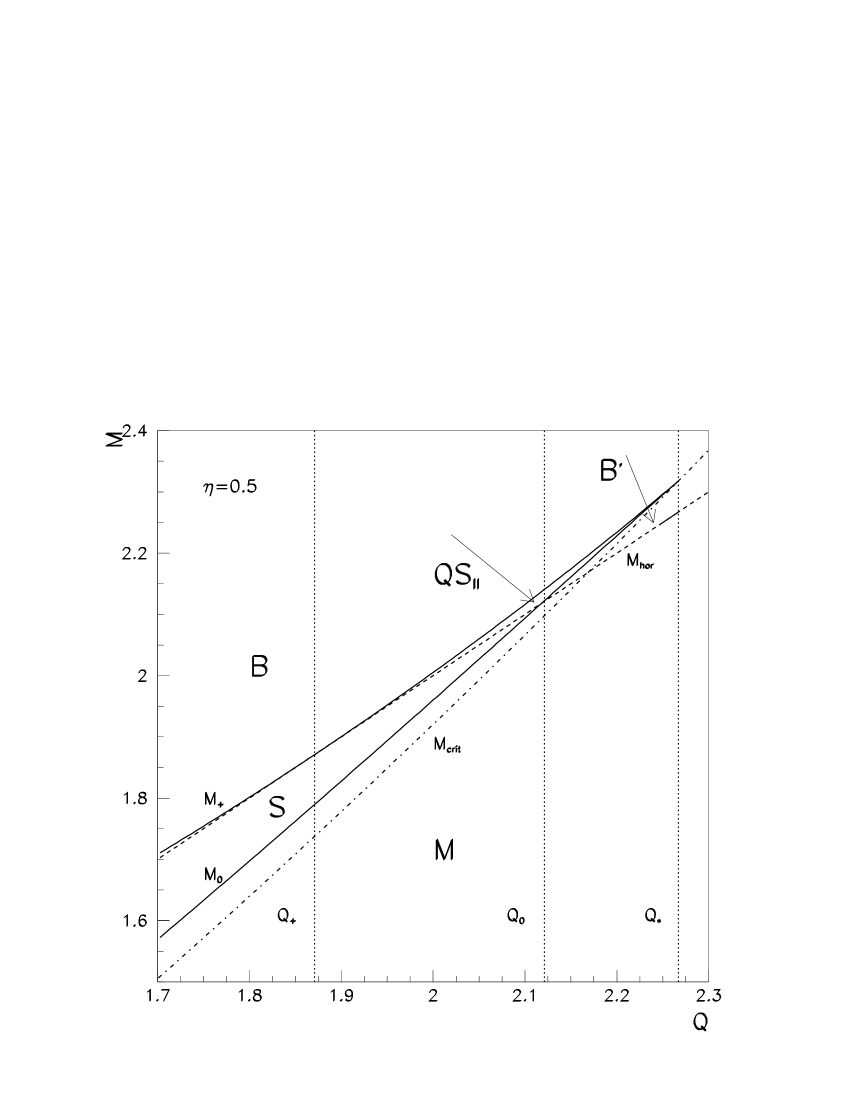
FIG. 3.: Zoom-in of the neighborhood of the bifurcation point $Q_{*}$ on Fig. 1. The parameter regime ${\it B}^{\prime}$ is indicated.

FIG. 4.: Zoom-out of Fig. 1. For clarity, the curve $M_{0}$ is not indicated.

FIG. 5.: Plot of the effective potential $U(z)$ vs. $z$ for $\eta=0.5$ corresponding to values of $Q$ and $M$ lying on the boundaries $M_{\cal M}$, $M_{0}$, $M_{+}$ and at the bifurcation point, $M_{*}$: (a) $M_{\cal M}$ ($Q=7.0$, $M=13.4028$); (b) $M_{0}$ ($Q=2.1307$, $M=2.1351$); (c) $M_{+}$ ($Q=2.0$, $M=2.0$); (d) the bifurcation point $M_{*}$ ( $Q_{*}=2.2671$, $M_{*}=2.3181$). The Reissner-Nordström horizons are located at $R_{+}$ and $R_{-}$. The domain of positive $\beta_{D}$ ($\beta_{M}$) is indicated at the top (bottom) of each plot.

FIG. 6.: $Q_{*}$, $Q_{0}$ and $Q_{+}$ vs. $\eta$

FIG. 7.: The trajectory type ${\cal O}$ occuring in the parameter regime ${\it S}$ embedded on (a) Gibbons-Hawking diagram for de Sitter spacetime; (b) Penrose diagram for Reissner-Norsdtröm spacetime ($M<Q$)

FIG. 8.: The trajectories ${\cal O}_{I}$ and ${\it B}_{I}$ occuring in parameter regime ${\it QSI}$ embedded on (a) Gibbons-Hawking diagram; (b) Penrose-Carter diagram ($M>Q$).

FIG. 9.: A trajectory of type ${\cal O}_{II}$ occuring in parameter regime ${\it QSII}$, and a trajectory of type ${\cal B}$ occuring in parameter regime ${\it B}$ (which includes ${\it QSII}$) embedded on (a) Gibbons-Hawking diagram; (b) Penrose-Carter diagram.

FIG. 10.: A trajectory of type ${\cal B}^{\prime}$ occuring in parameter regime ${\it B}^{\prime}$ embedded on (a) Gibbons-Hawking diagram; (b) Penrose-Carter diagram.

FIG. 11.: A trajectory of type ${\cal M}$ occuring in parameter regime ${\it M}$ embedded on (a) Gibbons-Hawking diagram; (b) Penrose-Carter diagram ($M>Q$).

- [1] A. Linde, Phys. Lett. B327, 208 (1994).
- [2] A. Vilenkin, Phys. Rev. Lett. 72, 3137 (1994).
- [3] E. Guendelman and A. Rabinowitz, Phys. Rev. D44, 3152 (1991).
- [4] S. K. Blau, E. I. Guendelman and A. H. Guth, Phys. Rev. D35, 1747 (1987).
- [5] Alan Guth, The Inflationary Universe (Addison-Wesley, Reading, MA. 1997).
- [6] M. Barriola and A. Vilenkin, Phys. Rev. Lett. 63, 341 (1989).
- [7] D. Harari and C. Lousto, Phys. Rev. D42, 2626 (1990).
- [8] G. W. Gibbons, in Proceedings of the XII Autum School on the Physical Universe, Lisbon, 1990, edited by J.D. Barrow et al., Lecture Notes in Physics Vol. 383 (Springer Verlag, Berlin, 1991).
- [9] M. E. Ortiz, Phys. Rev. D45, R2586 (1992).
- [10] P. Breitenlohner, P. Forgacs and D. Maison, Nucl. Phys. B383, 357 (1992); ibid. B442, 126 (1995).
- [11] N. Sakai, H. A. Shinkai, T. Tachizawa, and K. Maeda, Phys. Rev. D53, 655 (1996); ibid. D54, 2981 (1996).
- [12] N. Sakai, Phys. Rev. D54, 1548 (1996).
- [13] I. Cho and J. Guven, Phys. Rev. D58, 63502 (1998).
- [14] P. A. M. Dirac, Proc. R. Soc. A 268, 57 (1962).
- [15] T. Tachizawa, K. Maeda and T. Torii, Phys. Rev. D51, 4054 (1995).
- [16] K. Lee, V. P. Nair and E. Weinberg, Phys. Rev. D45, 2751 (1992).
- [17] G. L. Alberghi, D. A. Lowe and M. Trodden, JHEP 9902:020 (1999).
- [18] For a rigorous justification of this approximation in the context of a domain wall, see B. Carter and R. Gregory, Phys. Rev. D51, 5839 (1995).
- [19] B. Carter, Phys. Lett. 21, 423 (1966).
- [20] P. K. Townsend, Black Holes, Lecture Notes, gr-qc/9707012.
- [21] See, for example, W. Israel, in ‘Black Holes, Classical and Quantum’ (Mazatlán, Mexico, 1998).
- [22] E. Farhi and A. H. Guth, Phys. Lett. B183, 149 (1987).
- [23] E. Farhi, A. Guth and J. Guven, Nucl. Phys. B339, 417 (1990).
- [24] This is consistent with the general results of D. Sudarsky and R. Wald, Phys. Rev. D47, 5209 (1993); ibid. D46, 1453 (1992).
- [25] P. Hasenfratz and J. Kuti, Phys. Rep. 40, 75 (1978); P. Gnadig, Z. Kunszt, P. Hasenfratz, and J. Kuti, Annals of Phys. 116, 380 (1978).
- [26] A. Goldhaber, Phys. Rev. Lett. 63, 2158 (1989).