Quantum Isotropization of the Universe

Abstract

We consider minisuperspace models constituted of Bianchi I geometries with a free massless scalar field. The classical solutions are always singular (with the trivial exception of flat space-time), and always anisotropic once they begin anisotropic. When quantizing the system, we obtain the Wheeler-DeWitt equation as a four-dimensional massless Klein-Gordon equation. We show that there are plenty of quantum states whose corresponding bohmian trajectories may be non-singular and/or presenting large isotropic phases, even if they begin anisotropic, due to quantum gravitational effects. As a specific example, we exhibit field plots of bohmian trajectories for the case of gaussian superpositions of plane wave solutions of the Wheeler-DeWitt equation which have those properties. These conclusions are valid even in the absence of the scalar field.

I Introduction

Two of the main questions one might ask in cosmology are:

1) Is the Universe eternal or it had a beginning, and in the last case, was this beginning given by an initial singularity?

2) Why the Universe we live in is remarkably homogeneous and isotropic, with very small deviations from this highly symmetric state?

The answer given by classical General Relativity (GR) to the first question, indicated by the singularity theorems [1], asserts that probably the Universe had a singular beginning. As singularities are out of the scope of any physical theory, this answer invalidates any description of the very beginning of the Universe in physical terms. One might think that GR and/or any other matter field theory must be changed under the extreme situations of very high energy density and curvature near the singularity, rendering the physical assumptions of the singularity theorems invalid near this point. One good point of view (which is not the only one) is to think that quantum gravitational effects become important under these extreme conditions. We should then construct a quantum theory of gravitation and apply it to cosmology. For instance, in the euclidean quantum gravity approach [2] to quantum cosmology, a second answer to the first question comes out: the Universe may have had a non-singular birth given by the beginning of time through a change of signature.

In the same way, the naive answer of GR and the standard cosmological scenario to the second question is not at all satisfactory: the reason for the Universe be highly homogeneous and isotropic is a matter of initial conditions. However, solutions of Einstein’s equations with this symmetry are of measure zero; so, why the Universe is not inhomogeneous and/or anisotropic? Inflation [3, 4] is an idea that tries to explain this fact. Nevertheless, in order for inflation to happen, some special initial conditions are still necessary, although much more less stringent than in the case without inflation. Once again, quantum cosmology can help in this matter by providing the physical reasons for having the initial conditions for inflation.

Recently, many papers have been devoted to the application of the Bohm-de Broglie interpretation of quantum mechanics [5, 6] to quantum cosmology [7, 8, 9, 10, 11, 12, 13, 14, 15, 16]. One of the aims of these papers was to try to give an answer to the first question within a new perspective in quantum cosmology. In the framework of the Bohm-de Broglie interpretation of quantum mechanics applied to minisuperspace models, it was shown in References [11, 12, 13, 14, 15] that quantum gravitational effects may indeed become important under extreme situations of very high energy density and curvature, and avoid the initial singularity of the classical models. The solutions that come out are then non-singular (eternal) cosmological models, but with a very hot phase, tending to the usual classical solutions when the energy scales become smaller than the Planck scale. Of course this is a much better answer than the one given by classical GR.

The aim of this paper, as a natural sequence of the references cited above, is to address the second question from the point of view of the Bohm-de Broglie interpretation of quantum cosmology. We want to investigate if quantum mechanical effects can isotropize an anisotropic cosmological model yielding an alternative mechanism for the isotropization of the Universe. Our strategy is to take classical anisotropic models which never isotropizes, quantize them, and examine if quantum effects can at least create isotropic phases. As we will see, quantum effects can not only create isotropic phases but they can also isotropize the models forever, for a large variety of quantum states. Other authors have also studied this problem, mainly taking Bianchi IX models, adopting other interpretations of quantum cosmology, and they arrive at similar results [17, 18, 19, 20, 21].

The mathematical models we take are Bianchi I models with and without matter. For the case without matter, one of the anisotropic degrees of freedom is suppressed and we end with a two-dimensional minisuperspace model. The classical solutions of this case are all singular and always anisotropic, with the trivial exception of flat space-time. When quantizing this system we find that the solutions of the Wheeler-DeWitt can be written in terms of superpositions of plane wave solutions. Taking gaussian superpositions we show that there are bohmian trajectories representing universes expanding from an initial singularity and others representing bouncing non-singular universes, both with isotropic phases during the course of their evolutions. There are also bohmian non-singular periodic solutions with periodic isotropic phases and non-singular bouncing solutions which are never isotropic. For the case with matter, we take a minimally coupled scalar field with arbitrary coupling constant $\omega$. The minisuperspace is four-dimensional. The classical solutions are again singular, and once they begin anisotropic they continue to be anisotropic forever. When quantizing the system, we arrive at a Wheeler-DeWitt equation which corresponds to a massless Klein-Gordon equation in four dimensions. We show that there are plenty of spherical wave solutions whose bohmian trajectories represent expanding universes that isotropizes permanently after some period, many of them which are also non-singular. gaussian superpositions also present this feature.

The paper is organized as follows: in the next section we present the minisuperspace models which we will investigate and their classical solutions. In section III we quantize these models, and obtain their corresponding Wheeler-DeWitt equations and general quantum solutions. In section IV we present the results concerning the quantum isotropization of those solutions through the investigation of the bohmian trajectories we obtain from them. We end up in section V with conclusions and discussions.

II The classical minisuperspace model

Let us take the lagrangian

$${\it L}=\sqrt{-g}e^{-\phi}\biggr{(}R-w\phi_{;\rho}\phi^{;\rho}\biggl{)}\;.$$ (1)

For $w=-1$ we have effective string theory without the Kalb-Ramond field. For $w=-3/2$ we have a conformally coupled scalar field. Performing the conformal transformation $g_{\mu\nu}=e^{\phi}{\bar{g}}_{\mu\nu}$ we obtain

$${\it L}=\sqrt{-g}\biggr{[}R-C_{w}\phi_{;\rho}\phi^{;\rho}\biggl{]}\;,$$ (2)

where the bars have been omitted, and $C_{w}\equiv(\omega+\frac{3}{2})$. The cases of interest correspond to $C_{w}>0$.

The gravitational part of the minisuperspace model we study in this paper is given by the homogeneous and anisotropic Bianchi I line element

$$ds^{2} = -N^{2}(t)dt^{2}+\exp[2\beta_{0}(t)+2\beta_{+}(t)+2\sqrt{3}\beta_{-}(t)]\;dx^{2}+$$ (4)

$$\exp[2\beta_{0}(t)+2\beta_{+}(t)-2\sqrt{3}\beta_{-}(t)]\;dy^{2}+\exp[2\beta_{0}(t)-4\beta_{+}(t)]\;dz^{2}\;.$$

This line element will be isotropic if and only if $\beta_{+}(t)$ and $\beta_{-}(t)$ are constants [1]. Inserting Equation (4) into the action $S=\int{{\it L\,}d^{4}x}$, supposing that the scalar field $\phi$ depends only on time, discarding surface terms, and performing a Legendre transformation, we obtain the following minisuperspace classical hamiltonian

$$H=\frac{N}{24\exp{(3\beta_{0})}}(-p_{0}^{2}+p_{+}^{2}+p_{-}^{2}+p_{\phi}^{2})\;,$$ (5)

where $(p_{0},p_{+},p_{-},p_{\phi})$ are canonically conjugate to $(\beta_{0},\beta_{+},\beta_{-},\phi)$, respectively, and we made the trivial redefinition $\phi\rightarrow\sqrt{C_{w}/6}\;\;\phi$.

We can write this hamiltonian in a compact form by defining $y^{\mu}=(\beta_{0},\beta_{+},\beta_{-},\phi)$ and their canonical momenta $p_{\mu}=(p_{0},p_{+},p_{-},p_{\phi})$, obtaining

$$H=\frac{N}{24\exp{(3y^{0})}}\eta^{\mu\nu}p_{\mu}p_{\nu}\;,$$ (6)

where $\eta^{\mu\nu}$ is the Minkowski metric with signature $(-+++)$. The equations of motion are the constraint equation obtained by varying the hamiltonian with respect to the lapse function $N$

$${\cal H}\equiv\eta^{\mu\nu}p_{\mu}p_{\nu}=0\;,$$ (7)

and the Hamilton’s equations

$$\dot{y}^{\mu}=\frac{\partial{\cal H}}{\partial p_{\mu}}=\frac{N}{12\exp{(3y_{0})}}\eta^{\mu\nu}p_{\nu}\;,$$ (8)

$$\dot{p}_{\mu}=-\frac{\partial{\cal H}}{\partial y^{\mu}}=0\;.$$ (9)

The solution to these equations in the gauge $N=12\exp(3y_{0})$ is

$$y^{\mu}=\eta^{\mu\nu}p_{\nu}t+C^{\mu}\;,$$ (10)

where the momenta $p_{\nu}$ are constants due to the equations of motion and the $C^{\mu}$ are integration constants. We can see that the only way to obtain isotropy in these solutions is by making $p_{1}=p_{+}=0$ and $p_{2}=p_{-}=0$, which yields solutions that are always isotropic, the usual Friedmann-Robertson-Walker (FRW) solutions with a scalar field. Hence, there is no anisotropic solution in this model which can classically becomes isotropic during the course of its evolution. Once anisotropic, always anisotropic. If we suppress the $\phi$ degree of freedom, the unique isotropic solution is flat space-time because in this case the constraint (7) enforces $p_{0}=0$.

To discuss the appearance of singularities, we need the Weyl square tensor $W^{2}\equiv W^{\alpha\beta\mu\nu}W_{\alpha\beta\mu\nu}$. It reads

$$W^{2}=\frac{1}{432}e^{-12\beta_{0}}(2p_{0}p_{+}^{3}-6p_{0}p_{-}^{2}p_{+}+p_{-}^{4}+2p_{+}^{2}p_{-}^{2}+p_{+}^{4}+p_{0}^{2}p_{+}^{2}+p_{0}^{2}p_{-}^{2})\;.$$ (11)

Hence, the Weyl square tensor is proportional to $\exp{(-12\beta_{0})}$ because the $p$’s are constants (see Equations (9)), and the singularity is at $t=-\infty$. The classical singularity can be avoided only if we set $p_{0}=0$. But then, due to Equation (7), we would also have $p_{i}=0$, which corresponds to the trivial case of flat space-time. Therefore, the unique classical solution which is non-singular is the trivial flat space-time solution.

III Quantization of the classical model

The Dirac quantization procedure yields the Wheeler-DeWitt equation through the imposition of the condition

$$\hat{{\cal H}}\Psi=0\;,$$ (12)

on the quantum states, with $\hat{{\cal H}}$ defined as in Equation (7) (we are assuming the covariant factor ordering) using the substitutions

$$p_{\mu}\rightarrow-i\frac{\partial}{\partial y^{\mu}}\;.$$ (13)

Equation (12) reads

$$\eta^{\mu\nu}\frac{\partial^{2}}{\partial y^{\mu}y^{\nu}}\Psi(y^{\mu})=0\;.$$ (14)

A The empty model

In a first and simple example, we will freeze two degrees of freedom: the matter degree of freedom $y^{3}=\phi=0$, and one of the anisotropic degrees of freedom, $y^{2}=\beta_{-}=0$. We obtain a two-dimensional Klein-Gordon equation whose general solution is

$$\Psi(\beta_{0},\beta_{+})=\int{\{F(k)\exp[ik(\beta_{0}+\beta_{+})]+G(k)\exp[ik(\beta_{0}-\beta_{+})]\}dk}\;,$$ (15)

with $F(k)$ and $G(k)$ arbitrary functions of $k$. Let us take gaussian superpositions

$$F(k)=G(-k)=\exp\biggr{[}-\frac{(k-d)^{2}}{\sigma^{2}}\biggl{]}\;,$$ (16)

where $\sigma$ and $d$ are constants. In this case the wave function reads [23]

$$\Psi_{1}=\sigma\sqrt{\pi}\biggl{\{}\exp\biggl{[}-\frac{(\beta_{0}+\beta_{+})^{2}\sigma^{2}}{4}\biggr{]}\exp[id(\beta_{0}+\beta_{+})]+\exp\biggl{[}-\frac{(\beta_{0}-\beta_{+})^{2}\sigma^{2}}{4}\biggr{]}\exp[-id(\beta_{0}-\beta_{+})]\biggr{\}}\;.$$ (17)

For the case where

$$F(k)=G(k)=\exp\biggr{[}-\frac{(k+d)^{2}}{\sigma^{2}}\biggl{]}\;,$$ (18)

the wave function turns out to be

$$\Psi_{2}=\sigma\sqrt{\pi}\biggl{\{}\exp\biggl{[}-\frac{(\beta_{0}+\beta_{+})^{2}\sigma^{2}}{4}\biggr{]}\exp[-id(\beta_{0}+\beta_{+})]+\exp\biggl{[}-\frac{(\beta_{0}-\beta_{+})^{2}\sigma^{2}}{4}\biggr{]}\exp[-id(\beta_{0}-\beta_{+})]\biggr{\}}\;.$$ (19)

In the next section we will calculate the bohmian trajectories corresponding to the solutions (17,19) and see if there are isotropic phases in these quantum models.

B The scalar field model

In the general case of the four-dimensional minisuperspace model, we will investigate spherical-wave solutions of Equation (14). They read

$$\Psi_{3}=\frac{1}{y}\biggl{[}f(y^{0}+y)+g(y^{0}-y)\biggr{]}\;,$$ (20)

where $y\equiv\sqrt{\sum_{i=1}^{3}(y^{i})^{2}}$.

One particular example is the gaussian superposition of plane wave solutions of Equation (14),

$$\Psi_{4}(y^{\mu})=\int{\{F(\vec{k})\exp[i(|\vec{k}|y^{0}+\vec{k}.\vec{y})]+G(\vec{k})\exp[i(|\vec{k}|y^{0}-\vec{k}.\vec{y})]\}d^{3}k}\;,$$ (21)

where $\vec{k}\equiv(k_{1},k_{2},k_{3})$, $\vec{y}\equiv(y^{1},y^{2},y^{3})$, $|\vec{k}|\equiv\sqrt{\sum_{i=1}^{3}(k_{i})^{2}}$, with $F(\vec{k})$ and $G(\vec{k})$ given by

$$F(\vec{k})=G(\vec{k})=\exp\biggr{[}-\frac{(|\vec{k}|-d)^{2}}{\sigma^{2}}\biggl{]}\;.$$ (22)

After performing the integration in Equation (21) using spherical coordinates we obtain [23]

$$\Psi_{4}(y^{0},y) = \frac{i\pi^{3/2}}{y}\biggl{\{}[2d\sigma+i(y^{0}-y)\sigma^{3}]\exp\biggl{[}-\frac{(y^{0}-y)^{2}\sigma^{2}}{4}\biggr{]}\exp[id(y^{0}-y)]\biggl{[}1+\Phi\biggl{(}\frac{d}{\sigma}+i(y^{0}-y)\frac{\sigma}{2}\biggr{)}\biggr{]}$$ (24)

$$-[2d\sigma+i(y^{0}+y)\sigma^{3}]\exp\biggl{[}-\frac{(y^{0}+y)^{2}\sigma^{2}}{4}\biggr{]}\exp[id(y^{0}+y)]\biggl{[}1+\Phi\biggl{(}\frac{d}{\sigma}+i(y^{0}+y)\frac{\sigma}{2}\biggr{)}\biggr{]}\biggr{\}}\;,$$

where $\Phi(x)\equiv(2/\sqrt{{\pi}})\int_{0}^{x}\exp(-t^{2})dt$ is the probability integral. The wave function $\Psi_{4}$ is a spherical solution with the form of Equation (20) with $g=-f$. In order to simplify $\Psi_{4}$, we will take the limit $\sigma^{2}>>d$ and $(y^{0}\pm y)\sigma>>1$ in Equation (24) yielding [23]

$$f(z)\approx-\frac{16\pi d}{\sigma^{2}z^{3}}+i2\pi\biggl{(}\frac{2}{z^{2}}+\sigma^{2}\biggr{)}\;.$$ (25)

IV The quantum bohmian trajectories and results

In this section, we will apply the rules of the Bohm-de Broglie interpretation to the wave functions we have obtained in the previous section. We first summarize these rules for the case of homogeneous minisuperspace models. In this case, the general minisuperspace Wheeler-DeWitt equation is

$${\cal H}[{\hat{p}}_{\alpha}(t),{\hat{q}}^{\alpha}(t)]\Psi(q)=0\;,$$ (26)

where $p_{\alpha}(t)$ and $q^{\alpha}(t)$ represent the homogeneous degrees of freedom coming from the gravitational and matter fields. Writing $\Psi=R\exp(iS/\hbar)$, and substituting it into (26), we obtain the equation

$$\frac{1}{2}f^{\alpha\beta}(q^{\mu})\frac{\partial S}{\partial q^{\alpha}}\frac{\partial S}{\partial q^{\beta}}+U(q^{\mu})+Q(q^{\mu})=0\;,$$ (27)

where

$$Q(q^{\mu})=-\frac{1}{2R}f^{\alpha\beta}\frac{\partial^{2}R}{\partial q^{\alpha}\partial q^{\beta}}\;.$$ (28)

The quantities $f^{\alpha\beta}(q^{\mu})$ and $U(q^{\mu})$ are the minisuperspace particularizations of the DeWitt metric [22], and of the scalar curvature density of the space-like hypersurfaces together with matter potential energies, respectively. The causal interpretation applied to quantum cosmology states that the trajectories $q^{\alpha}(t)$ are real, independently of any observations. Equation (27) is the Hamilton-Jacobi equation for them, which is the classical one amended with the quantum potential term (28), responsible for the quantum effects. This suggests to define

$$p_{\alpha}=\frac{\partial S}{\partial q^{\alpha}}\;,$$ (29)

where the momenta are related to the velocities in the usual way

$$p_{\alpha}=f_{\alpha\beta}\frac{1}{N}\frac{\partial q^{\beta}}{\partial t}\;,$$ (30)

and $f_{\alpha\beta}$ is the inverse of $f^{\alpha\beta}$. To obtain the quantum trajectories, we have to solve the following system of first order differential equations, called the guidance relations:

$$\frac{\partial S(q^{\gamma})}{\partial q^{\alpha}}=f_{\alpha\beta}\frac{1}{N}\frac{\partial q^{\beta}}{\partial t}\;.$$ (31)

Equations (31) are invariant under time reparametrization. Hence, even at the quantum level, different choices of $N(t)$ yield the same space-time geometry for a given non-classical solution $q^{\alpha}(t)$. There is no problem of time in the causal interpretation of minisuperspace quantum cosmology.

For the minisuperspace we are investigating, the guidance relations in the gauge $N=12\exp(3y_{0})$ are (see Equations (8))

$$p_{\mu}=\frac{\partial S}{\partial y^{\mu}}=\eta_{\mu\nu}{\dot{y}}^{\nu}\;,$$ (32)

where $S$ is the phase of the wave function.

A The empty model

Taking the phase of the solution (17), and inserting it into Equations (32), remembering that $y^{2}=\beta_{-}$ and $y^{3}=\phi$ have been suppressed, we get the following system of planar equations:

$$\dot{\beta}_{0}=\frac{\beta_{+}\sigma^{2}\sin(2d\beta_{0})+2d\sinh(\beta_{0}\beta_{+}\sigma^{2})}{2[\cos(2d\beta_{0})+\cosh(\beta_{0}\beta_{+}\sigma^{2})]}\;,$$ (33)

$$\dot{\beta}_{+}=\frac{2d\cos(2d\beta_{0})+2d\cosh(\beta_{0}\beta_{+}\sigma^{2})-\beta_{0}\sigma^{2}\sin(2d\beta_{0})}{2[\cos(2d\beta_{0})+\cosh(\beta_{0}\beta_{+}\sigma^{2})]}\;.$$ (34)

The line $\beta_{0}=0$ divides configuration space in two symmetric regions. The line $\beta_{+}=0$ contains all singular points of this system, which are nodes and centers. The nodes appear when the denominator of the above equations, which is proportional to the absolute value of the wave function, is zero. No trajectory can pass through them. They happen when $\beta_{+}=0$ and $\cos(2d\beta_{0})=-1$, or $\beta_{0}=(2n+1)\pi/2d$, $n$ an integer, with separation $\pi/d$. The center points appear when the numerators are zero. They are given by $\beta_{+}=0$ and $\beta_{0}=2d\,[{\rm cotan}(d\beta_{0})]/\sigma^{2}$. They are intercalated with the node points. As $\mid\beta_{0}\mid\rightarrow\infty$ these points tend to $n\pi/d$, and their separations cannot exceed $\pi/d$. As one can see from Equations (33) and (34), the classical solutions (10) are recovered when $\mid\beta_{0}\mid\rightarrow\infty$ and $\mid\beta_{+}\mid\rightarrow\infty$, the $\beta$’s become proportional to $t$. The quantum potential given in Equation (28), which now reads,

$$Q(\beta_{0},\beta_{+}) = -\frac{1}{2R}\biggl{(}-\frac{\partial^{2}R}{\partial\beta_{0}^{2}}+\frac{\partial^{2}R}{\partial\beta_{+}^{2}}\biggr{)}$$ (35)

$$= \frac{[\beta_{+}\sigma^{2}\sin(2d\beta_{0})+2d\sinh(\beta_{0}\beta_{+}\sigma^{2})]^{2}-[\beta_{0}\sigma^{2}\sin(2d\beta_{0})-2d\cos(2d\beta_{0})-2d\cosh(\beta_{0}\beta_{+}\sigma^{2})]^{2}}{8[\cos(2d\beta_{0})+\cosh(\beta_{0}\beta_{+}\sigma^{2})]^{2}}\;,$$ (36)

becomes negligible in these limits.

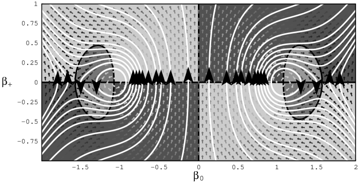
FIG. 1.: Field plot of the system of planar equations (33-34) for $\sigma=d=1$, which uses the Bohm-de Broglie interpretation with the wave function $\Psi_{1}$, Equation (17). Each arrow of the vector field is shaded according to its true length, black representing short vectors and white, long ones. The four shades of gray show the regions where the vector field is pointing to northeast, northwest, southeast or southwest. The black curves are the nullcline curves that separate these regions. The trajectories are the white curves with direction arrows.

A field plot of this planar system is shown in Figure 1 for $\sigma=d=1$. We can see plenty of different possibilities, depending on the initial conditions. Near the center points we can have oscillating universes without singularities and with periodic isotropic phases, with amplitude of oscillation of order $1$. For negative values of $\beta_{0}$, the universe arises classically from a singularity but quantum effects become important forcing it to recollapse to another singularity, recovering classical behaviour near it. Isotropic phases may happen near their maximum size. For positive values of $\beta_{0}$, the universe contracts classically but when $\beta_{0}$ is small enough quantum effects become important creating an inflationary phase which avoids the singularity. The universe contracts to a minimum size and after reaching this point it expands forever, recovering the classical limit when $\beta_{0}$ becomes sufficiently large. In this case isotropic phases may happen when the universe is near its minimum size. In both cases we see that isotropic phases happen only when quantum effects are important. We can see that, for $\beta_{0}$ negative, we have classical limit for small scale factor while for $\beta_{0}$ positive we have classical limit for big scale factor. In these models with $d=1$, the isotropic phases last very shortly. Only for $\mid d\mid<<1$ can the isotropic phases be arbitrarily large because, as said above, the separation of the singular points goes like $\pi/d$.

For the wave function $\Psi_{2}$, the analysis goes in the same way but we have to interchange $\beta_{0}$ with $\beta_{+}$ in Figure 1. In this case, we have also periodic solutions but the others are anisotropic universes arising classically from a singularity, experiencing quantum effects in the middle of their expansion when they become approximately isotropic, and recovering their classical behaviour for large values of $\beta_{0}$. Depending on the initial conditions, the isotropic phase can be arbitrarily large. There are no further possibilities.

B The scalar field model

Let us study the spherical wave solutions (20) of Equation (14). The guidance relations (32) are

$$p_{0}=\partial_{0}S=\Im\biggl{(}\frac{\partial_{0}\Psi_{3}}{\Psi_{3}}\biggr{)}=-{\dot{y}}^{0}\;,$$ (37)

$$p_{i}=\partial_{i}S=\Im\biggl{(}\frac{\partial_{i}\Psi_{3}}{\Psi_{3}}\biggr{)}={\dot{y}}^{i}\;,$$ (38)

where $S$ is the phase of the wave function. In terms of $f$ and $g$ the above equations read

$${\dot{y}}^{0}=-\Im\biggl{(}\frac{f^{\prime}(y^{0}+y)+g^{\prime}(y^{0}-y)}{f(y^{0}+y)+g(y^{0}-y)}\biggr{)}\;,$$ (39)

$${\dot{y}}^{i}=\frac{y^{i}}{y}\Im\biggl{(}\frac{f^{\prime}(y^{0}+y)-g^{\prime}(y^{0}-y)}{f(y^{0}+y)+g(y^{0}-y)}\biggr{)}\;,$$ (40)

where the prime means derivative with respect to the argument of the functions $f$ and $g$, and $\Im(z)$ is the imaginary part of the complex number $z$.

From Equations (40) we obtain that

$$\frac{dy^{i}}{dy^{j}}=\frac{y^{i}}{y^{j}}\;,$$ (41)

which implies that $y^{i}(t)=c_{j}^{i}y^{j}(t)$, with no sum in $j$, where the $c_{j}^{i}$ are real constants, $c_{j}^{i}=1/c_{i}^{j}$, and $c_{1}^{1}=c_{2}^{2}=c_{3}^{3}=1$. Hence, apart some positive multiplicative constant, knowing about one of the $y^{i}$ means knowing about all $y^{i}$. Consequently, we can reduce the four equations (39) and (40) to a planar system by writing $y=C|y^{3}|$, with $C>1$, and working only with $y^{0}$ and $y^{3}$, say. The planar system now reads

$${\dot{y}}^{0}=-\Im\biggl{(}\frac{f^{\prime}(y^{0}+C|y^{3}|)+g^{\prime}(y^{0}-C|y^{3}|)}{f(y^{0}+C|y^{3}|)+g(y^{0}-C|y^{3}|)}\biggr{)}\;,$$ (42)

$${\dot{y}}^{3}=\frac{{\rm sign}(y^{3})}{C}\Im\biggl{(}\frac{f^{\prime}(y^{0}+C|y^{3}|)-g^{\prime}(y^{0}-C|y^{3}|)}{f(y^{0}+C|y^{3}|)+g(y^{0}-C|y^{3}|)}\biggr{)}\;.$$ (43)

Note that if $f=g$, $y^{3}$ stabilizes at $y^{3}=0$ because ${\dot{y}}^{3}$ as well as all other time derivatives of $y^{3}$ are zero at this line. As $y^{i}(t)=c_{j}^{i}y^{j}(t)$, all $y^{i}(t)$ become zero, and the cosmological model isotropizes forever once $y^{3}$ reaches this line. Of course one can find solutions where $y^{3}$ never reaches this line, but in this case there must be some region where ${\dot{y}}^{3}=0$, which implies ${\dot{y}}^{i}=0$, and this is an isotropic region. Consequently, quantum anisotropic cosmological models with $f=g$ always have an isotropic phase, which can become permanent in many cases.

As a concrete example, let us take the gaussian $\Psi_{4}$ given in Equation (24). It is a spherical wave solution of the Wheeler-DeWitt equation (14) with $f=-g$, and hence it does not necessarily have isotropic phases as described above for the case $f=g$. Figure 2 shows a field plot of this system for $d/\sigma^{2}=-10^{-4}$ and $C=2$. In the region $|\phi|>>|\beta_{0}|$ we have periods of isotropic expansion because $\phi={\rm const.}$ implies $\beta_{\pm}={\rm const.}$. Depending on the value of $|\phi|$, this isotropic phase can be arbitrarily long. These trajectories are periodic and without singularities. Due to quantum effects, no trajectory crosses the point $\beta_{0}=\phi=0$. Figure 3 shows the bohmian trajectories for the wave function given in Equation (24), now with $d/\sigma^{2}=10^{-4}$ and $C=2$. They have some qualitative behaviours different from the precedent case. The isotropic phases, now in contraction, are no longer periodic. They are parts of universes that contract anisotropically from infinity, experience a period of isotropy, and contract anisotropically to a singularity. Figure 3 shows that no trajectories crosses the point $\beta_{0}=\phi=0$.

In order to get some analytical insight over Figures 2 and 3, we present the planar system obtained from the guidance relations corresponding to the wave function (24) in the approximation (25):

$${\dot{\beta}}_{0}=\frac{\frac{2d}{\sigma^{2}}(3\beta_{0}^{4}+6C^{2}\beta_{0}^{2}\phi^{2}-C^{4}\phi^{4})}{\beta_{0}^{2}(\beta_{0}^{2}-C^{2}\phi^{2})^{2}+\frac{4d^{2}}{\sigma^{4}}(3\beta_{0}^{2}+C^{2}\phi^{2})^{2}}\;,$$ (44)

$${\dot{\phi}}=\frac{\frac{16d}{\sigma^{2}}\beta_{0}^{3}\phi}{\beta_{0}^{2}(\beta_{0}^{2}-C^{2}\phi^{2})^{2}+\frac{4d^{2}}{\sigma^{4}}(3\beta_{0}^{2}+C^{2}\phi^{2})^{2}}\;,$$ (45)

where we have reset $y^{0}=\beta_{0}$ and $y^{3}=\phi$. This approximation is not reliable in the lines $\beta_{0}=\pm C\phi$. As one can see immediately from these equations, $\beta_{\pm}={\rm const.}$ whenever $|\phi|>>|\beta_{0}|$, and the sign of $d$ defines the trajectories direction.

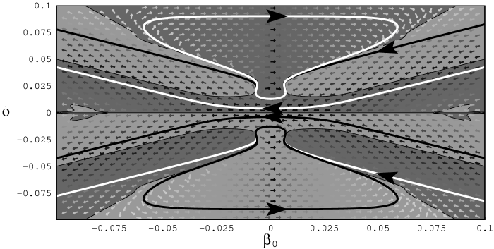
FIG. 2.: Field plot of the system of planar equations (42-43) for $\sigma=100$, $d=-1$ and $C=2$, which uses the Bohm-de Broglie interpretation with the wave function $\Psi_{4}$ given in Equation (24). Each arrow of the vector field is shaded according to its true length, black representing short vectors and white, long ones. The dark shade of gray shows the regions where the derivative of the vector field points clockwise (the light shade of gray means the opposite), and this shading allows to see the regions with arbitrarily long periods of isotropic expansion corresponding to periodic universes without singularities. There are also black or white curves with direction arrows corresponding to universes contracting from infinity to a singularity. Due to quantum effects, the trajectories do not cross the origin.

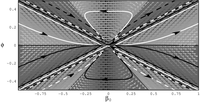
FIG. 3.: Field plot of the system of planar equations (42-43) for $\sigma=100$, $d=1$ and $C=2$, which uses the Bohm-de Broglie interpretation with the wave function $\Psi_{4}$, Equation (24). Each arrow of the vector field is shaded according to its true length, black representing short vectors and white, long ones. The dark shade of gray shows the regions where the derivative of the vector field points clockwise (the light shade of gray means the opposite) and this shading allows to see the regions with arbitrarily long periods of isotropic contraction. The trajectories are the black or white curves with direction arrows; they do not cross the origin due to quantum effects.

V Conclusion

Adopting the Bohm-de Broglie interpretation of quantum cosmology, we have shown that quantum effects can generate an efficient alternative mechanism for the isotropization of cosmological models. Anisotropic classical models which never isotropize may present arbitrarily large isotropic phases during the course of their evolutions if quantum effects are taken into account, without needing to introduce any classical inflationary phase. The models studied were Bianchi I models in empty space or filled with a free massless scalar field.

There are questions and developments which should be undertaken within this approach: the dependence of the above results on boundary conditions of the Wheeler-DeWitt equation, their generalizations to other Bianchi models, and the conditions for which quantum effects can also induce homogeneity on cosmological models which are classically inhomogeneous. The last issue is by far the most interesting but also the most complicated one because the implementation of the Bohm-de Broglie interpretation for inhomogeneous cosmological models is much more subtle and involved [16]. These questions will be the subject of our future investigations.

REFERENCES

- [1] S. W. Hawking and G. F. R. Ellis, The large scale structure of space-time (Cambridge University Press, Cambridge, 1973).
- [2] Euclidean Quantum Gravity, ed. by G. W. Gibbons and S. W. Hawking (World Scientific, London, 1993).
- [3] A. H. Guth, Phys. Rev. D28, 347 (1981).
- [4] E. W. Kolb and M. S. Turner, The Early Universe (Addison-Wesley Publishing Company, New York, 1990).
- [5] D. Bohm, Phys. Rev. 85, 166 (1952); D. Bohm, B. J. Hiley and P. N. Kaloyerou, Phys. Rep. 144, 349 (1987).
- [6] P. R. Holland, The Quantum Theory of Motion: An Account of the de Broglie-Bohm Causal Interpretation of Quantum Mechanics (Cambridge University Press, Cambridge, 1993).
- [7] J. C. Vink, Nucl. Phys. B369, 707 (1992).
- [8] J. Kowalski-Glikman and J. C. Vink, Class. Quantum Grav. 7, 901 (1990).
- [9] Y. V. Shtanov, Phys. Rev. D54, 2564 (1996).
- [10] A. Valentini, Phys. Lett. A158, 1, (1991).
- [11] J. A. de Barros and N. Pinto-Neto, Int. J. of Mod. Phys. D7, 201 (1998).
- [12] J. A. de Barros, N. Pinto-Neto and M. A. Sagioro-Leal, Phys. Lett. A241, 229 (1998).
- [13] J. A. de Barros, N. Pinto-Neto and M. A. Sagioro-Leal, to appear in GRG.
- [14] R. Colistete Jr., J. C. Fabris and N. Pinto-Neto, Phys. Rev. D57, 4707 (1998).
- [15] J. C. Fabris, N. Pinto-Neto and A. F. Velasco, gr-qc 9903111, to appear in Classical and Quantum Gravity.
- [16] N. Pinto-Neto and E. S. Santini, Phys. Rev. D59, 123517 (1999).
- [17] W. A. Wright and I. G. Moss, Phys. Lett. 154B, 115 (1985).
- [18] P. Amsterdamski, Phys. Rev. D31, 3073 (1985).
- [19] B. K. Berger and C. N. Vogeli, Phys. Rev. D32, 2477 (1985).
- [20] S. Del Campo and A. Vilenkin, Phys. Lett. B224, 45 (1989).
- [21] V. Moncrief and M. P. Ryan, Jr., Phys. Rev. D44, 2375 (1991).
- [22] B. S. DeWitt, Phys. Rev. 160, 1113 (1967).
- [23] I. S. Gradshteyn and I. M. Ryzhik, Table of Integrals, Series and Products (Academic Press, New York, 1980).