Coordinate singularities in harmonically-sliced cosmologies

Abstract

Harmonic slicing has in recent years become a standard way of prescribing the lapse function in numerical simulations of general relativity. However, as was first noticed by Alcubierre [Phys. Rev. D 55, 5981 (1997)], numerical solutions generated using this slicing condition can show pathological behaviour. In this paper, analytic and numerical methods are used to examine harmonic slicings of Kasner and Gowdy cosmological spacetimes. It is shown that in general the slicings are prevented from covering the whole of the spacetimes by the appearance of coordinate singularities. As well as limiting the maximum running times of numerical simulations, the coordinate singularities can lead to features being produced in numerically evolved solutions which must be distinguished from genuine physical effects.

I Introduction

In the 3+1 formulation of general relativity, the freedom in choosing a coordinate system through which to describe a spacetime is replaced by freedom in choosing two gauge quantities: the lapse function $N$, which controls the slicing of the spacetime into a foliation of spatial hypersurfaces, and the shift vector $N^{i}$, which defines a set of reference world lines threading those spatial slices. Numerical simulations based on the 3+1 formulation are required to prescribe a method for evaluating the lapse and the shift in terms of the geometrical quantities (the intrinsic metric $h_{ij}$ and the extrinsic curvature $K_{ij}$) and the matter fields (the density $\rho$, momentum $J^{i}$, and stress $S^{ij}$) that are known on each spatial slice. The use of a harmonic slicing condition to determine the lapse function is appealing for both practical and theoretical reasons, and the incorporation of such a slicing condition in numerical codes is becoming increasingly common. However, recent work (Alcubierre and Massó [1, 2], Geyer and Herold [3]) has found evidence that the use of harmonic slicing can produce pathological behaviour in numerically evolved spacetimes.

This paper addresses the question as to how suitable harmonic slicing is for work in numerical relativity. In section II the main features of the harmonic slicing condition are reviewed. Following an approach similar to that of Geyer and Herold [3, 4] the behaviour of ‘planar’ harmonic slicings of the Minkowski spacetime is analysed in section III; it is demonstrated there that such slicings always cover the whole of the spacetime. A similar statement does not however hold true for the Kasner spacetime. Results derived in section IV show that coordinate singularities of the type found by Alcubierre [1] appear in harmonic slicings of the Kasner spacetime under reasonably general conditions. Section V shows that, furthermore, the results for the Kasner spacetime carry over directly to harmonic slicings of the more general class of Gowdy $T^{3}$ spacetimes. In section VI results are presented from numerical simulations of the Kasner spacetime which use harmonic slicing. The coordinate singularities predicted by the analysis of earlier sections are indeed encountered, and the behaviour of the numerical solutions at times just prior to the formation of coordinate singularities is examined. Section VII concludes the discussion by considering the implications that these results have for the use of harmonic slicing in numerical relativity.

II Harmonic Slicing in Numerical Relativity

When considering Einstein’s equations as a 3+1 evolution system, a spacetime is described in terms of a foliation $\{\Sigma_{t}:t\in{\mathbb{R}}\}$ of spatial slices, which defines, in effect, a time coordinate $t$ on the spacetime. (The details of this idea are discussed by York [5], and familiarity with that material is assumed.) The manner in which a spacetime is sliced is a very important issue when the 3+1 formulation is used as a basis for performing numerical simulations. This section recalls some basic ideas on slicing conditions in numerical relativity and, in particular, describes how harmonic slicings of spacetimes are constructed.

Traditionally, work in numerical relativity has been based on maximal or constant mean curvature (CMC) slicing conditions, initially developed for this purpose by Eardley, Smarr and York [5, 6, 7], among others. A spatial slice has constant mean curvature if $K$, the trace of the extrinsic curvature tensor, takes a constant value on that slice. If values for $K$ are specified across a range of slices as a function of the time coordinate $t$, then the 3+1 evolution equation for the extrinsic curvature yields an elliptic equation determining the value of the lapse function $N$ on each slice:

$$\Delta N-N[K_{ij}K^{ij}+4\pi(\rho+S)]=-K^{\prime}(t)\,,$$ (1)

where $\Delta=h^{ij}\nabla_{\!i}\nabla_{\!j}$. If the function $K(t)$ is identically zero then the spacetime is maximally sliced. Maximal slicing has been found to work well in numerical simulations of asymptotically flat spacetimes, while for closed cosmologies (in which at most one maximal slice can exist) the more general CMC slicing condition is appropriate. Based on their behaviour in simple examples and their success in numerical simulations, it is believed that the maximal and CMC slicing conditions will in general produce foliations which cover most, if not all, of a spacetime being investigated, and which at the same time avoid getting too close to any singularities that may form in that spacetime.

Interest in the use of harmonic slicing has arisen in recent years because of its connection with work that has been done in reformulating Einstein’s equations as an explicitly hyperbolic system (see the review [8] by Reula). To date, all of the known 3+1 formulations of general relativity as a strongly hyperbolic evolution system with only physically relevant characteristic speeds determine the lapse through some form of the harmonic slicing condition.

Harmonic slicing contrasts in several basic ways with maximal and CMC slicing. The lapse function $N$ in a harmonically-sliced spacetime is determined either through an algebraic condition or a simple evolution equation, and not through an elliptic condition as in equation (1). This ‘local’ specification of the lapse is a great advantage from the point of view of implementing a numerical code to evolve solutions to Einstein’s equations since elliptic partial differential equations are computationally very expensive to solve. The harmonic slicing condition also differs from the maximal and CMC slicing conditions in that it specifies a relationship between two adjacent slices in a foliation rather than determining properties of each individual slice: while an isolated spacetime slice can be characterized as maximal or of constant mean curvature, there is no such thing as an individual harmonic slice. One consequence of this is that the choice of lapse function on the initial slice of a foliation is arbitrary if the harmonic slicing condition is used.

To simplify the following discussion, all spacetime foliations considered in this paper are assumed to have shift vectors $N^{i}$ which are identically zero. Since the shift vector controls only the positioning of spatial coordinates on slices and not how the slices themselves are arranged, this assumption does not limit the generality of the results derived here on the appearance of coordinate singularities.

The harmonic slicing condition for determining the lapse $N$ can be expressed in either algebraic form,

$$N=Q(t,x^{k})\sqrt{\det h_{ij}}\,,$$ (2)

or as an evolution equation,

$${\partial N\over\partial t}=N(\ln Q)_{,t}-N^{2}K\,,$$ (3)

where the slicing density $Q(t,x^{i})$ is an arbitrary (positive) function of the foliation coordinates which does not depend on any evolved variables. If the slicing density is independent of the foliation time coordinate $t$, then the harmonic slicing is described as simple, and in this case a choice of the value of the lapse $N$ on an initial slice completely determines the value of the slicing density $Q$. The alternative situation is described as generalized harmonic slicing, and it is clear from equation (2) that any spacetime foliation can be constructed using generalized harmonic slicing and a particular form for the slicing density $Q$. If the slicing density has only a ‘separable’ dependence on the time coordinate of the form $Q(t,x^{i})=f(t)\bar{Q}(x^{i})$, then the resultant foliation has the same slices as the foliation produced by using $\bar{Q}(x^{i})$ as the slicing density, but with the slices labelled by a different time coordinate. In general it is not obvious how a useful slicing density $Q$ which has a non-trivial dependence on the time coordinate $t$ may be chosen, and so the simple form of harmonic slicing is most often used in practice.

The main question addressed in this paper is that of how suitable the harmonic slicing condition is for numerical work. Several authors have already considered this question from various different viewpoints. Bona and Massó [9] have shown that the (simple) harmonic slicing condition can be used to foliate several standard spacetimes, and also that ‘focusing singularities’ are avoided by the slicing condition in much the same way as they are in maximally-sliced spacetimes, with the slices of the foliation not reaching the singularity in a finite coordinate time. (It should be noted that for a harmonically-sliced spacetime a focusing singularity is essentially a point at which the lapse $N$ becomes zero—this is in contrast to the behaviour found at the ‘gauge pathologies’ described below.) Cook and Scheel [10] have investigated the construction of well-behaved harmonic foliations for Kerr-Newmann black hole spacetimes.

The work of Alcubierre and Massó [1, 2] is of particular relevance to the present discussion. They have shown that ‘gauge pathologies’ (described as ‘coordinate shocks’ in the earlier paper) can occur in numerical simulations based on hyperbolic formulations of Einstein’s equations which use harmonic slicing. (In fact, a range of gauge conditions are considered by the authors, with simple harmonic slicing—the only gauge choice of interest here—corresponding to the special case $f=1$ in their formulation. None of the alternative gauge choices they use correspond to the generalized harmonic slicing condition.) These gauge pathologies manifest as a loss of continuity at points in the evolved solution with, in particular, large spikes appearing in the lapse. After the time at which the pathologies appear the numerical solution no longer converges at the expected order. Alcubierre and Massó explain the appearance of gauge pathologies in terms of nonlinear behaviour in the hyperbolic evolution equations. However this fails to adequately answer questions about how common the gauge pathologies are, what happens to the foliation at the points where pathologies appear, and what approaches can be used to prevent the pathologies from occurring.

Simple harmonic slicings for the Schwarzschild and Oppenheimer-Snyder spacetimes have been investigated by Geyer and Herold [3, 4]. The approach they use is based on an alternative representation of equations (2) and (3) in the simple harmonic case: if $T$ is a scalar function on a spacetime, the level surfaces of which represent the spatial slices of a foliation $\{\Sigma_{T}\}$, then the spacetime will be harmonically sliced (in the simple sense) if

$$\Box T\equiv g^{\mu\nu}\nabla_{\!\mu}\nabla_{\!\nu}T=0\,.$$ (4)

By numerically integrating equation (4) with respect to known background metrics, Geyer and Herold construct simple harmonic slicings which they compare to maximal slicings of the spacetimes. Some properties of a slicing can be determined straightforwardly from its time function $T$, and in particular the lapse $N$ can be evaluated through the equation

$$g^{\mu\nu}(\nabla_{\!\mu}T)(\nabla_{\!\nu}T)=-1/N^{2}\,,$$ (5)

where it is clear that the vector field normal to the foliation must remain timelike if the lapse is to have a positive real value. In fact, Geyer and Herold [3] find that for simple harmonic slicings of the Oppenheimer-Snyder spacetime, foliations which are initially timelike can at later times become null or spacelike, with the development of the foliation thus terminating at what it seems appropriate to call a coordinate singularity. The lapse becomes infinite as these singular points are reached, and this is consistent with the behaviour found at the gauge pathologies of Alcubierre and Massó.

In what follows, Geyer and Herold’s approach is applied to Minkowski, Kasner and Gowdy spacetimes, with the intention being to gain a better understanding of the circumstances under which coordinate singularities appear, and in particular to determine whether they are a rare or a common feature of harmonic slicings.

III Harmonic Slicings of the Minkowski Spacetime

In the present work, equations (4) and (5) are used to investigate the formation of coordinate singularities in (simple) harmonic slicings of cosmological models. The following approach is employed. The metric $g_{\mu\nu}$ of the spacetime being investigated is assumed to be known with respect to a coordinate system $(t,x,y,z)$. An alternative foliation of the spacetime is constructed by taking as an initial slice one of the constant time hypersurfaces of the background coordinate system: the foliation time coordinate $T(t,x,y,z)$ is given an initial value

$$T(t_{0},x,y,z)=t_{0}\,,$$ (6)

for some value $t_{0}$ of the coordinate $t$. (It is assumed here that the hypersurface $t=t_{0}$ is spacelike.) The lapse function of the foliation can be specified arbitrarily on the initial slice and this determines via equation (5) the value of the first derivative of $T$ away from that slice:

$$T_{,t}(t_{0},x,y,z)={1\over N_{0}(x,y,z)\sqrt{-g^{00}(t_{0},x,y,z)}}\,.$$ (7)

Equations (6) and (7) provide initial data for the wave equation (4), and the solution $T$ describes a new simple harmonic slicing of the spacetime.

As an example of how equation (4) can be used to find coordinate singularities, consider harmonic foliations of the Minkowski spacetime, written in standard coordinates as

$\displaystyle g_{\mu\nu}dx^{\mu}dx^{\nu}=-dt^{2}+dx^{2}+dy^{2}+dz^{2}\,.$

Suppose that a ‘planar’ slicing of the spacetime is constructed such that the time function $T$ depends only on the Minkowski coordinates $t$ and $x$. Then equation (4) takes the form of the one-dimensional wave equation

$\displaystyle T_{,tt}=T_{,xx}\,,$

which has the general solution

$\displaystyle T(t,x)=f(t+x)+h(t-x)\,,$

for arbitrary functions $f(u)$ and $h(u)$. The lapse associated with this time function can be found from equation (5):

$$-1/N^{2} = T_{,x}{}^{2}-T_{,t}{}^{2}$$

$$= -4f^{\prime}(t+x)h^{\prime}(t-x)\,,$$

and the lapse will be well behaved as long as the function $f^{\prime}(t+x)h^{\prime}(t-x)$ is positive.

For most problems the next step in the analysis would be to use equations (6) and (7) to specify a value for the lapse on an initial slice of the foliation. However the present case is sufficiently simple that the appearance of coordinate singularities can be studied without needing to specify an initial slice. If the lapse becomes infinite at a point in the foliation then the function $f^{\prime}(t+x)h^{\prime}(t-x)$ must be zero there, and it is clear that the function must then be zero at all points along a line $t+x=\hbox{\it constant\/}$ or $t-x=\hbox{\it constant\/}$. Consequently, any spacelike slice of that foliation must include a point in it at which the lapse is infinite. It follows that for simple harmonic slicings of the ‘planar’ Minkowski spacetime no coordinate singularities will be present, and the foliation will cover the whole of the spacetime, provided that the initial slice of the foliation is everywhere spacelike. (This result is consistent with the numerical simulations of Minkowski spacetime reported on by Alcubierre [1]. No gauge pathologies are discovered for ‘planar’ harmonic slicings—the $f=1$ case—of flat spacetime, although they are found in the spherically symmetric case.)

In the following sections a similar analysis is performed for more complicated spacetimes, and coordinate singularities are found to be much more common than the above result for the Minkowski spacetime would suggest.

IV Harmonic Slicings of the Kasner Spacetime

In this section, equation (4) is used to construct simple harmonic foliations of the Kasner spacetime, with the main point of interest being the question of whether or not coordinate singularities (gauge pathologies in the terminology of Alcubierre and Massó [2]) form in the slicings. Later, in section VI, these results are compared to numerical simulations of the spacetime.

The present work uses the axisymmetric Kasner model described by the metric

$$ds^{2}=t^{-1/2}(-dt^{2}+dx^{2})+t\,(dy^{2}+dz^{2})\,,$$ (8)

for which a cosmological singularity is present at time $t=0$. For convenience in the following analysis (and to strengthen the connection with the Gowdy cosmologies examined in section V) a three-torus topology is imposed on the Kasner spacetime: periodicity is assumed in each of the coordinates $x$, $y$ and $z$ over the range $[0,2\pi)$.

As in the simple example for the Minkowski spacetime given in the previous section, here ‘planar’ slicings of the Kasner spacetime are considered for which the time function $T$ depends only on the coordinates $t$ and $x$. A straightforward calculation then shows that for the metric (8), equation (4) for the time function of a harmonically-sliced foliation is equivalent to

$$T_{,tt}-T_{,xx}+t^{-1}T_{,t}=0\,.$$ (9)

This equation can be solved by decomposing $T$ spatially as a sum of Fourier modes (recalling that, since the model is spatially closed, the function $T$ must be periodic in the coordinate $x$) and the general solution is found to be

$$T = a_{0}\ln t+b_{0}$$ (11)

$${}+\sum_{n=1}^{\infty}\bigl{[}Z_{+n}\!(t)\cos(nx)+Z_{-n}\!(t)\sin(nx)\bigr{]}\,,$$

with

$\displaystyle Z_{\pm n}\!(t)=a_{\pm n}J_{0}(|n|t)+b_{\pm n}Y_{0}(|n|t)\hbox{ \ \ for }n\neq 0\,,$

where $a_{\pm n}$ and $b_{\pm n}$ are constants, and $J_{\nu}$ and $Y_{\nu}$ are Bessel functions of the first and second kinds [11].

Equation (5) for the lapse function $N$ of the foliation can be written in the present case as

$$\sqrt{t}\,(T_{,t}{}^{2}-T_{,x}{}^{2})=1/N^{2}\,,$$ (12)

and the requirement that the foliation be well behaved can then be expressed as

$$T_{,t}>|T_{,x}|\,,$$ (13)

where it is assumed that the orientation of the time function $T$ of the foliation is the same as that of the Kasner time $t$, and thus that $T_{,t}$ is positive. If the time function $T$ of equation (11) fails to satisfy the condition (13) at a point, then the harmonic slicing must have a coordinate singularity there.

The constants $a_{\pm n}$ and $b_{\pm n}$ in equation (11) can be determined by specifying a value $N_{0}(x)$ for the lapse on an initial hypersurface $t=t_{0}$ as in equations (6) and (7). In fact, rather than choosing the initial value for the lapse directly, it is more convenient to choose an initial value $I(x)$ for the time derivative of $T$, with this being specified as a Fourier sum,

$$T_{,t}(t_{0},x) = I(x)$$ (14)

$$= k_{0}+\sum_{n=1}^{\infty}\bigl{[}k_{+n}\cos(nx)+k_{-n}\sin(nx)\bigr{]}\,,$$ (15)

where the constants $k_{\pm n}$ must be such that $I(x)$ is everywhere positive. The value of the lapse on the initial slice can then be determined through equation (7):

$\displaystyle N_{0}(x)={1\over t_{0}{}^{1/4}I(x)}\,.$

The particular time function $T$ of equation (11) which fits the initial data of equations (6) and (14) is found to be

$$T=t_{0}+k_{0}t_{0}\ln(t/t_{0})-{\pi t_{0}\over 2}\sum_{n=1}^{\infty}\bigl{[}J_{0}(nt)Y_{0}(nt_{0})-Y_{0}(nt)J_{0}(nt_{0})\bigr{]}\bigl{[}k_{+n}\cos(nx)+k_{-n}\sin(nx)\bigr{]}\,.$$ (16)

The simplest harmonic foliations of the Kasner metric (8) are the homogeneous ones for which the time function $T$ is independent of the coordinate $x$. Then, to within a linear rescaling, the function $T$ equals $\ln t$, and so the cosmological singularity in the spacetime occurs in the harmonic foliation only in the limit as $T$ tends to negative infinity. Clearly the foliation covers the entire Kasner spacetime and contains no coordinate singularities.

The behaviour of homogeneous harmonic slicings is, however, not representative of the general case. As an example, figure 1 shows the foliation which results from setting the lapse on the initial slice to be

$$N_{0}(x)={1\over{\textstyle 1+{1\over 2}\sin x}}\qquad\hbox{for }t_{0}=1\,,$$ (17)

which corresponds to the choice of non-zero coefficients $k_{0}=1$ and $k_{-1}=1/2$ in equation (14). When equation (12) is evaluated to determine the lapse on this foliation, it is found that in some spacetime regions to the future of the initial slice the quantity $1/N^{2}$ is non-positive; figure 2, which plots $1/N^{2}$, is filled in where this happens. Coordinate singularities must appear in any slices of the foliation which intersect these regions, and the development of the foliation cannot proceed beyond a time $T=T_{\text{sing}}\simeq 2.45$ with the lapse $N$ tending to infinity at points as the limiting slice is approached. In contrast, if the foliation is extended backwards in time from the initial slice towards the cosmological singularity, then the lapse appears to be well behaved on all of the slices.

It can in fact be shown that, in general, harmonic foliations of the Kasner spacetime always develop coordinate singularities at sufficiently late (future) times. If the time derivative of the function in equation (16) is evaluated at a fixed spatial coordinate $x=x_{0}$, then

$\displaystyle T_{,t}(t,x_{0})={k_{0}t_{0}\over t}+{\pi t_{0}\over 2}\sum_{n=1}^{\infty}n\,c_{n}(x_{0})\bigl{[}J_{1}(nt)Y_{0}(nt_{0})-Y_{1}(nt)J_{0}(nt_{0})\bigr{]}\,,$

where it is assumed that the value $x_{0}$ has been chosen such that at least one of the values $c_{n}$ is non-zero. For sufficiently large values of the coordinate $t$, the approximations (9.2.5) and (9.2.6) of reference [11] can be applied to the Bessel functions in this equation. The result is that

$\displaystyle T_{,t}(t,x_{0})\simeq{k_{0}t_{0}\over t}+\sqrt{\pi\over 2\,t}t_{0}\sum_{n=1}^{\infty}\sqrt{n}\,c_{n}\bigl{[}Y_{0}(nt_{0})\cos(nt-{\textstyle{3\over 4}}\pi)-J_{0}(nt_{0})\sin(nt-{\textstyle{3\over 4}}\pi)\bigr{]}={k_{0}t_{0}\over t}+{\Theta(t)\over\sqrt{t}}\,,$

where $\Theta(t)$ is a periodic function which takes both positive and negative values. It follows that, for some sufficiently large value of the coordinate $t$, the value of $T_{,t}$ must be negative at a point. Since this violates the condition (13), it must be the case that a coordinate singularity is present in the foliation.

The above argument shows that coordinate singularities must in general appear in harmonic slicings of an expanding Kasner cosmology but gives no indication of how much of the spacetime a slicing will cover before it becomes pathological. To investigate this, consider the simple case of a time function $T$ from equation (16) which, like the foliation produced by the initial data (17), contains only one non-trivial mode of amplitude $k$:

$$T = t_{0}+k_{0}t_{0}\ln(t/t_{0})$$ (19)

$${}-k{\pi t_{0}\over 2}\bigl{[}J_{0}(nt)Y_{0}(nt_{0})-Y_{0}(nt)J_{0}(nt_{0})\bigr{]}\sin(nx)\,,$$

where $0<k<k_{0}$. For a fixed value of the Kasner time $t$ the foliation will be well behaved (in that condition (13) is satisfied) if and only if

$\displaystyle{k_{0}t_{0}\over t}>{kn\pi t_{0}\over 2}\max_{x}\bigl{\{}|A(t)\cos(nx)|-B(t)\sin(nx)\bigr{\}}\,,$

where

$$A(t) = J_{0}(nt)Y_{0}(nt_{0})-Y_{0}(nt)J_{0}(nt_{0})\,,$$

$$B(t) = J_{1}(nt)Y_{0}(nt_{0})-Y_{1}(nt)J_{0}(nt_{0})\,,$$

and this condition is equivalent to

$$F(t)\equiv t^{2}\bigl{[}A(t)^{2}+B(t)^{2}\bigr{]}<\left({2k_{0}\over kn\pi}\right)^{2}\,.$$ (20)

It is straightforward to show that $F^{\prime}(t)\geq 0$. Furthermore, if the time $t$ is assumed to be large enough for approximations [11] to be applied to the Bessel functions in $A(t)$ and $B(t)$, then $F(t)\simeq t\,\Pi(t)$ where $\Pi(t)$ is a positive, periodic function. An estimate of the time $t=t_{\text{sing}}$ at which a coordinate singularity develops can then be seen to obey

$$t_{\text{sing}}\propto(k_{0}/k)^{2}\,,$$ (21)

and so, for a harmonic slicing which is perturbed from homogeneity by a single mode of amplitude $k$, the amount of the spacetime covered by the slicing becomes infinite as $k$ tends to zero.

Considering now the behaviour of the slicing in the region of spacetime between the initial slice and the cosmological singularity, it follows from equation (20) that, for the single mode case (19), coordinate singularities never appear. To see this, note that the function $F(t)$ must satisfy the inequality at time $t=t_{0}$ since the lapse is required to be well behaved on the initial slice, and since it is an increasing function of time it must then also satisfy the inequality at all earlier times. In the limit as $t$ tends to zero (while $x$ is constant), the Bessel function behaviour is known from equations (9.1.10–13) of reference [11], and the time function $T$ must have the form

$$T \sim t_{0}\bigl{[}k_{0}+kJ_{0}(nt_{0})\cos(nx)\bigr{]}\ln t$$ (23)

$${}+\hbox{(terms that tend to a constant)}\,.$$

Since the factor multiplying $\ln t$ is always positive, the value of $T$ must tend to negative infinity as the cosmological singularity is approached. Thus a single mode harmonic slicing will always cover the whole of the Kasner spacetime to the past of the initial slice.

Returning to the general case in which an arbitrary number of modes are present in the time function $T$, the above argument can be used to derive a simple condition on the initial data (14) which ensures that a slicing is well behaved in the region of spacetime between the initial slice and the cosmological singularity. Suppose that equation (16) is split up as

$\displaystyle T=t_{0}+\sum_{n=1}^{\infty}\left(T^{(+n)}+T^{(-n)}\right)\,,$

where

$$T^{(+n)} = k_{0}^{(+n)}t_{0}\ln(t/t_{0})-k_{+n}{\pi t_{0}\over 2}\bigl{[}J_{0}(nt)Y_{0}(nt_{0})-Y_{0}(nt)J_{0}(nt_{0})\bigr{]}\cos(nx)\,,$$

$$T^{(-n)} = k_{0}^{(-n)}t_{0}\ln(t/t_{0})-k_{-n}{\pi t_{0}\over 2}\bigl{[}J_{0}(nt)Y_{0}(nt_{0})-Y_{0}(nt)J_{0}(nt_{0})\bigr{]}\sin(nx)\,,$$

and the values $k^{(\pm n)}_{0}$ are arbitrary subject to the condition

$\displaystyle\sum_{n=1}^{\infty}\left(k_{0}^{(+n)}+k_{0}^{(-n)}\right)=k_{0}\,.$

The condition (13) that the foliation be free of coordinate singularities will then certainly be satisfied if

$\displaystyle T^{(+n)}{}_{\!,t}>|T^{(+n)}{}_{\!,x}|\quad\hbox{and}\quad T^{(-n)}{}_{\!,t}>|T^{(-n)}{}_{\!,x}|\quad\forall n\,,$

and, as the analysis of the single mode case shows, this will be true for $0<t<t_{0}$ if it is true for $t=t_{0}$. The time derivative of each function $T^{(\pm n)}$ must therefore be positive on the initial hypersurface $t=t_{0}$, and for this to be the case the values $k_{0}^{(\pm n)}$ must be chosen such that

$\displaystyle k^{(+n)}_{0}>|k_{+n}|\quad\hbox{and}\quad k^{(-n)}_{0}>|k_{-n}|\quad\forall n\,.$

This can always be done if

$$k_{0}>\sum_{n=1}^{\infty}\bigl{(}|k_{+n}|+|k_{-n}|\bigr{)}\,,$$ (24)

and so any initial value for the lapse which satisfies this condition must produce a foliation which is free of coordinate singularities to the past of the initial slice. In addition to this, if the behaviour of the time function $T$ is considered as $t$ tends to zero, then it is straightforward to show (in analogy with equation (23) for the single mode case) that condition (24) ensures that $T$ tends to negative infinity for all values of $x$ as the cosmological singularity is approached, and hence that the foliation covers all of the spacetime up to the singularity. The condition (24) on the initial lapse is sufficient but not necessary for the harmonic foliation to be well behaved to the past of the initial slice. In fact, experimentation with different choices of initial data (14) suggests that, even when condition (24) is not satisfied, harmonic foliations may never develop coordinate singularities as the cosmological singularity is approached, although no proof (or disproof) of this conjecture has yet been constructed.

V Harmonic Slicings of Inhomogeneous Cosmologies

To summarize the results of the previous section, foliations of the Kasner spacetime (8) based on the simple harmonic slicing condition (4) have been investigated under the assumptions that one slice of the foliation coincides with a $t=\hbox{\it constant\/}$ hypersurface of the original metric, and that the foliation is independent of two of the standard spatial coordinates. It is found that when the Kasner cosmology is expanding, the slices of the foliation must eventually develop coordinate singularities (except when the lapse is initially constant), with this happening at late times for foliations which are initially close to homogeneous. In contrast, when the Kasner cosmology is collapsing, the results suggest that coordinate singularities never develop in the foliation and that the slices extend all the way to the cosmological singularity. (This is certainly true if the lapse on the initial slice is chosen such that the coefficients of equation (14) satisfy the condition (24), and it may in fact be the case for all reasonable choices of initial lapse.)

The behavioural differences found in harmonic foliations according to whether the Kasner spacetime is expanding or collapsing can be explained by considering the relationship between the lapse function $N$ and the mean curvature $K$ of a slice. In any foliation, the mean curvature provides a measure of the local convergence of world lines running normal to the spatial slices:

$$K=-\nabla_{\!\mu}n^{\mu}=-\pounds_{\!n}\bigl{(}{\textstyle\ln\sqrt{\det h_{ij}}}\bigr{)}\,,$$ (25)

where $n^{\mu}$ is the vector normal to the slices, $\pounds_{\!n}$ is the Lie derivative along that vector, and $\sqrt{\det h_{ij}}$ is the spatial volume element. The value of $K$ is positive when the foliation world lines are locally converging, and negative when they are expanding. The harmonic slicing condition can be written in terms of the mean curvature of the foliation using equation (3):

$\displaystyle{\partial(1/N)\over\partial t}=K\,,$

where the harmonic slicing is assumed to be simple with zero shift. It follows that when the mean curvature $K$ is positive (as it may be expected to be for slices of a collapsing cosmology) the value of $1/N$ will increase, and so the lapse will approach (but usually not reach) zero. (The ability of the harmonic slicing condition to avoid ‘focusing singularities’ at which the lapse vanishes is discussed by Bona and Massó [9].) Conversely, when the mean curvature is negative (as it typically will be in an expanding spacetime) the value of $1/N$ will decrease, and if it reaches zero then a coordinate singularity of the type investigated in this paper will develop in the foliation.

The obvious extension of the above analysis is to the consideration of harmonic slicings of spacetimes more general than the Kasner model. In fact it turns out to be straightforward to extend the results of section IV to a class of inhomogeneous cosmological models [12]: the unpolarized Gowdy spacetimes on $T^{3}$ (the three-torus). These spacetimes are vacuum models of spatially closed cosmologies with planar symmetry, and can be represented by the metric

$$ds^{2} = e^{\lambda/2}t^{-1/2}(-dt^{2}+d\theta^{2})$$ (27)

$${}+e^{P}t\bigl{[}d\sigma^{2}+2Q\,d\sigma\,d\delta+(Q^{2}+e^{-2P})\,d\delta^{2}\bigr{]}\,.$$

The spatial coordinates $\theta$, $\sigma$ and $\delta$ range from $0$ to $2\pi$. A cosmological singularity occurs at time $t=0$ and the model expands forever through positive values of $t$. The functions $\lambda$, $P$ and $Q$ depend on the coordinates $\theta$ and $\tau$ only and are required by the topology of the model to be periodic in $\theta$. The vacuum Einstein equations for the metric (27) reduce to evolution and constraint equations for the variables $P$, $Q$ and $\lambda$ which cannot in general be solved exactly. Moncrief [13] has shown that no singularities appear in the Gowdy $T^{3}$ spacetimes for $0<t<+\infty$, and that this coordinate range describes the maximal Cauchy development of the models. Thus, no coordinate singularities of the type investigated in this paper can be present in the standard Gowdy slicing.

If the analysis of the previous section for harmonic slicings of the axisymmetric Kasner spacetime (8) is applied to the Gowdy metric (27) (taking the planar symmetry of the slicing to coincide with the symmetry of the metric) then it is found that the time function $T$ must satisfy

$\displaystyle T_{,tt}-T_{,\theta\theta}+t^{-1}T_{,t}=0\,,$

while the lapse $N$ of the associated foliation is defined through

$\displaystyle e^{-\lambda(t,\theta)/2}\sqrt{t}\bigl{(}T_{,t}{}^{2}-T_{,\theta}{}^{2}\bigr{)}=1/N^{2}\,.$

Comparing these expressions to equations (9) and (12), it is clear that the Gowdy $T^{3}$ spacetimes admit the same harmonic foliations as the axisymmetric Kasner spacetime, and furthermore that the condition that foliations must satisfy to be free of coordinate singularities is the same. It thus turns out that all of the results summarized above on the behaviour of harmonic slicings of a Kasner cosmology carry over directly to a fairly general class of planar cosmological models. (In addition, it may be noted that the class of Gowdy spacetimes on $T^{3}$ includes as special cases the full set of Kasner spacetimes with the same topology. Thus the restriction of the discussion in section IV to only the axisymmetric Kasner model (8) can be relaxed; the same results hold for all of the Kasner spacetimes.)

VI Numerical Simulations of the Kasner Spacetime

The results of section IV show that coordinate singularities are a generic feature of harmonic foliations of the (expanding, axisymmetric) Kasner cosmology. It follows then that numerical simulations of that spacetime which use the harmonic slicing condition will be forced to terminate after a finite number of time steps, regardless of their accuracy. The practical details of this are examined in the present section.

Numerical simulations are performed based on initial data for the Kasner spacetime given by the metric (8) on an initial slice at time $t=t_{0}=1$ using the harmonic slicing condition (2) and the initial value (17) for the lapse. The foliation of the Kasner spacetime which results is the one pictured in figure 1, and the numerical simulation thus allows the prediction made in section IV—that coordinate singularities prevent the foliation from developing beyond a time $T=T_{\text{sing}}\simeq 2.45$—to be verified. The slicing density of the foliation is given the inhomogeneous form

$$Q(T,X,Y,Z)={t_{0}{}^{-3/4}\over 1+{1\over 2}\sin X}\,,$$ (28)

where $(T,X,Y,Z)$ is the coordinate system of the numerical simulation, and is distinct from the coordinate system $(t,x,y,z)$ of the original Kasner metric except on the initial slice which is labelled $T=t_{0}$ and on which $(X,Y,Z)=(x,y,z)$. The shift vector $N^{i}$ is taken to be identically zero, and the lack of dependence of the slicing density $Q$ on the foliation time $T$ means that the harmonic slicing is of the simple type. All of the quantities involved in the numerical simulation are independent of the spatial coordinates $Y$ and $Z$ so that the evolved spacetime in effect has planar symmetry. The numerical simulation is one dimensional and uses a high-resolution numerical scheme within an adaptive mesh refinement code to evolve a first-order hyperbolic formulation of the vacuum Einstein equations; a complete description of the code is given in reference [14].

Figure 3 displays the $(T,X)$ coordinate system of the numerical simulation as it appears in the $(t,x)$ coordinates of the homogeneous background metric (8). This comparison between coordinate systems is made using an algorithm, described in reference [14], for tracking the positions of the observers at rest in the slices of the foliation, based on the values $N(T,X)$ taken by the lapse during the course of the simulation. The observer world lines are plotted up until a simulation time $T=2.3$. Although the inaccuracies in the numerical solution which are present at that time are not sufficient to stop the simulation, they do make it increasingly difficult to accurately track the positions of the observers. The $T=\hbox{\it constant\/}$ surfaces reconstructed in figure 3 can be seen to be in good agreement with the exact results shown in figure 1.

The analysis of section IV (as presented in figures 1 and 2) shows that at a time $T=T_{\text{sing}}\simeq 2.45$ the lapse $N$ must become infinite at points of the evolved foliation. Figure 4 shows the actual value taken by the lapse at the earlier time $T=2.3$ in the simulation, and it can be seen that two sharp spikes are already present in the solution. As the evolution progresses these spikes grow in size, and if the evolved solution were exact they would reach infinite heights within a short time. As they grow, the two spikes also narrow and become closer together. The reason for this can be seen from the paths of the coordinate observers plotted in figure 3: in the region $0<x<\pi$ where the coordinate singularities eventually form, the world lines normal to the foliation are diverging (with respect to the background coordinates), and so the region is resolved by a diminishing number of grid points. It should be noted that this divergence of observers is not itself the cause of the coordinate singularities; it could in principle be counteracted by an appropriate choice of shift vector for the foliation, but this would not prevent the lapse from becoming infinite. The narrowing and effective coalescence of the spikes is problematic for the simulation since features which are smaller than the grid spacing $\Delta X$ cannot be accurately resolved, and, regardless of the number of grid points used, eventually the numerical solution must fail to accurately model the behaviour of the exact solution. In fact, with the spikes being inadequately resolved, the evolved value of the lapse fails to become infinite (or even the computer representation of this) as the coordinate singularities are reached, and it is possible for the simulation to continue beyond the time at which the slices of the foliation cease to be spacelike in the exact solution. However, the numerical solution has no physical meaning past the points at which coordinate singularities form, and in particular, as noted by Alcubierre and Massó [2], it will no longer converge as the grid is refined.

The spikes that develop in the lapse as the coordinate singularities are approached are at face value very similar to some features that are seen in numerical solutions for collapsing one- and two-dimensional inhomogeneous cosmologies, as studied by Hern and Stewart [14, 15]. In both cases spiky features appear in the evolved variables which, as the simulation progresses, increase in height and decrease in width until they can no longer be resolved by the numerical grid used in the simulation. The question then arises as to whether the features seen in the inhomogeneous cosmologies have any physical relevance or whether they are, like the features in the Kasner simulation described above, entirely a coordinate effect.

In reference [14] it is concluded that the spiky features found in the inhomogeneous cosmological models are not simply artifacts of the coordinate systems (or the metric variables) on which the simulations are based. Part of the evidence for this comes from an examination of the profiles of the evolved variables with respect to proper distances rather than coordinate distances: the narrowing of the spiky features becomes even more pronounced when proper distances are used. It is interesting to note that the opposite result is observed when a similar analysis is applied to the spikes seen in the lapse in figure 4. If the metric component $h_{11}$, which measures the proper distance in the $X$-direction of the simulation, is examined for the data plotted in figure 4, it is found that sharp spikes (towards positive infinity) are coincident there with the spikes in the lapse, and hence that the apparently narrow spikes are in fact spread over large physical distances. As figure 5 demonstrates, if instead of being plotted against the coordinate $X$, the lapse is shown as a function of the proper distance along the $X$-axis, then the spikes no longer appear as notable features of the solution. This approach could prove to be a useful way of distinguishing genuine physical features in an evolved solution from effects caused by coordinate singularities in harmonic slicings.

VII Discussion

It has been demonstrated in sections IV and V of this paper that ‘planar’ foliations of Kasner and Gowdy $T^{3}$ cosmologies generated using the simple harmonic slicing condition will, except in special cases, always terminate at coordinate singularities without covering the whole of the spacetimes. When these analytic results are considered together with the descriptions of coordinate singularities in specific examples of ‘spherically symmetric’ harmonic foliations given by Alcubierre [1], and Geyer and Herold [3], a pessimistic picture of the nature of the harmonic slicing condition emerges: it appears likely that, except in special cases, foliations generated by harmonic slicing will eventually terminate at coordinate singularities. (Seemingly this pathological behaviour can occur whenever the foliation locally undergoes a protracted period of expansion).

The coordinate singularities examined here arise as part of exact solutions for harmonically-sliced spacetimes, and they cannot be avoided simply by employing alternative numerical methods in simulations. This is clearly a drawback to the use of harmonic slicing in numerical work, and by extension to the use of hyperbolic formulations of Einstein’s equations which typically rely on this type of slicing. It should be appreciated however that no known slicing condition is guaranteed to completely cover an arbitrary spacetime, and potential problems with coordinate singularities do not necessarily outweigh the advantages of using hyperbolic formulations in numerical relativity. In section VI the behaviour of a numerically evolved solution is examined as it approaches a coordinate singularity, and it is found that by considering measures of proper distance it may be possible to distinguish the effects of coordinate singularities from genuine physical features of a spacetime. In general though the most reliable approach to identifying the presence of a coordinate singularity in a numerical solution is the one recognized by Alcubierre and Massó [2]: convergence of the solution is lost when a coordinate singularity develops.

Of course, the formation of coordinate singularities has only been discussed here for the simple harmonic slicing condition, and it is possible that the freedom in choosing the time dependence of the slicing density in generalized harmonic slicing could be put to use in controlling the development of the spacetime foliation such that coordinate singularities are avoided. Although when used in the context of a hyperbolic formulation the slicing density is formally required to be independent of the evolved variables, in practice there seems to be no problem in allowing occasional ‘corrections’ to be made to its value in response to the behaviour of the foliation; in effect this amounts to intermittently halting the simulation and choosing a new value for the lapse on the current slice. (An important point here is that changes to the slicing density should be made only at fixed time intervals, rather than after a fixed number of time steps, since otherwise the exact solution being sought will depend on the resolution of the simulation.) This ‘piecewise harmonic’ form of slicing has been used in some preliminary tests employing simple heuristics for making alterations to the value of the slicing density, with the resulting foliations being examined using the world line integration algorithm which was used to produce figure 3. (The algorithm was in fact developed for this purpose.) As yet however no definite conclusions regarding the effectiveness of this approach have been reached.

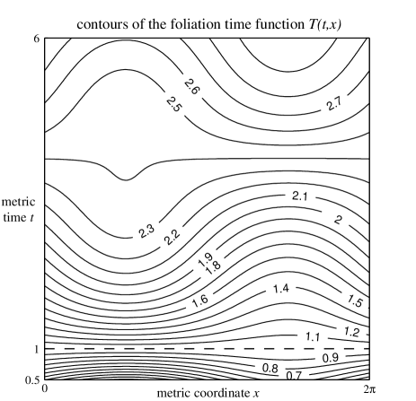
FIG. 1.: A simple harmonic foliation as seen in the background Kasner metric. The initial slice of the foliation coincides with the $t=1$ hypersurface of the metric (8) and is given an inhomogeneous initial lapse (17). The time function $T$ is evaluated from equation (16) and presented as a contour plot with respect to the coordinates $(t,x)$ of the original metric. The contours represent slices of the foliation with the dashed line marking the position of the initial slice.

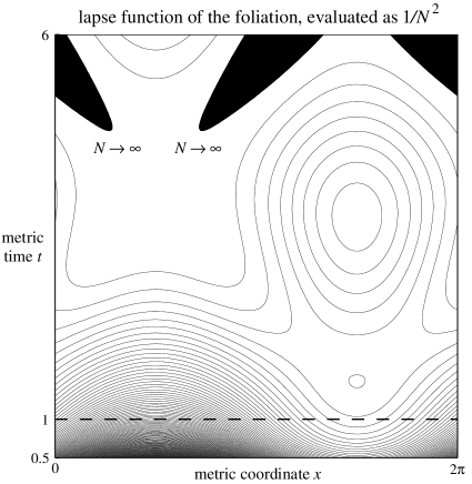
FIG. 2.: Lapse function for the harmonic foliation of figure 1. The lapse $N$ is evaluated from the foliation time T through equation (12) and presented with respect to the coordinates $(t,x)$ of the background Kasner metric (8). Evenly spaced contours of the function $1/N^{2}$ are shown. The filled-in regions at the top of the plot show where $1/N^{2}$ ceases to be a positive function, and thus where coordinate singularities must appear in the slices of the foliation. As in figure 1, the dashed line marks the position of the initial slice.

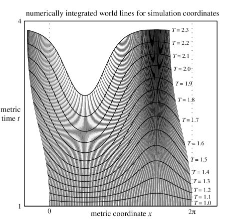
FIG. 3.: Coordinate world lines for a numerical simulation as seen in the background Kasner metric. A homogeneous initial data set is numerically evolved using harmonic slicing based on the inhomogeneous gauge function (28). The world lines of the simulation’s grid points are tracked relative to the coordinate system $(t,x)$ of the background metric (8) using the numerical values produced for the lapse function. Two hundred grid points are evenly spaced on the $t=1$ hypersurface of the background metric at the initial simulation time $T=1$, and the paths they subsequently follow are plotted up until the end of the simulation at time $T=2.3$. Periodicity of the spatial domain means that observers who ‘go off’ at $x=0$ will ‘come on’ at $x=2\pi$. This plot is to be compared with figure 1.

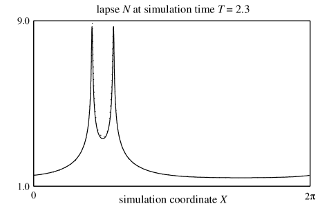
FIG. 4.: Lapse function for the inhomogeneously-sliced Kasner spacetime. The solid line shows the value of the lapse $N$ at the final time of the numerical simulation presented in figure 3. Coordinate singularities are responsible for the sharp spikes in the data. (The dotted line shows an alternative value for the lapse evaluated indirectly by combining the estimated world line positions of figure 3 with the analytic lapse values plotted in figure 2; the results of both approaches can be seen to be in good agreement.)

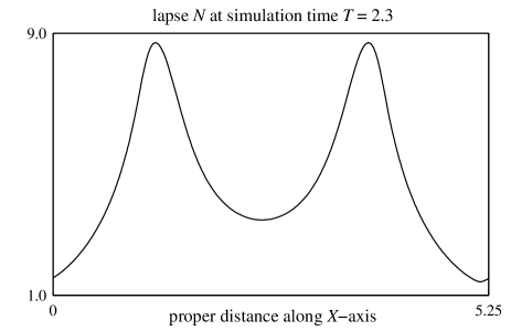
FIG. 5.: The lapse from figure 4 is re-plotted against proper distance in the $X$-direction. The peaks which in the original plot appear very sharp are found to be quite smooth when viewed with respect to a physical measure of distance. (The proper distance is measured starting from the point $X=0$, and an orbit of the evolved spacetime at time $T=2.3$ is found to have a proper length of approximately $5.25$.)

- [1] M. Alcubierre, Phys. Rev. D 55, 5981–5991 (1997).
- [2] M. Alcubierre and J. Massó, Phys. Rev. D 57, 4511–4515 (1998).
- [3] A. Geyer and H. Herold, Gen. Relativ. Gravit. 29, 1257–1268 (1997).
- [4] A. Geyer and H. Herold, Phys. Rev. D 52, 6182–6185 (1995).
- [5] J. W. York, in Sources of Gravitational Radiation, edited by L. Smarr (Cambridge University Press, 1979).
- [6] L. Smarr and J. W. York, Phys. Rev. D 17, 2529–2551 (1978).
- [7] D. M. Eardley and L. Smarr, Phys. Rev. D 19, 2239–2259 (1979).
- [8] O. A. Reula, “Hyperbolic Methods for Einstein’s Equations,” Living Review, http:// www.livingreviews.org/Articles/Volume1/1998-3reula/ .
- [9] C. Bona and J. Massó, Phys. Rev. D 38, 2419–2422 (1988).
- [10] G. B. Cook and M. A. Scheel, Phys. Rev. D 56, 4775–4781 (1997).
- [11] M. Abramowitz and I. A. Stegun, Handbook of Mathematical Functions (Dover Publications Inc., 1964), Chapter 9.
- [12] R. H. Gowdy, Ann. Phys. (N.Y.) 83, 203–241 (1974).
- [13] V. Moncrief, Ann. Phys. (N.Y.) 132, 87–107 (1981).
- [14] S. D. Hern, Ph.D. thesis, Cambridge University, 1999.
- [15] S. D. Hern and J. M. Stewart, Class. Quantum Grav. 15, 1581–1593 (1998).