TIME DISPERSION AND EFFICIENCY OF DETECTION FOR SIGNALS IN GRAVITATIONAL WAVE EXPERIMENTS

Using simulated signals and measured noise with the EXPLORER and NAUTILUS detectors we find the efficiency of signal detection and the signal arrival time dispersion versus the signal-to-noise ratio.

1 Introduction

There are today five detectors of gravitational waves (GW) in operation [1, 2, 3, 4, 5], all of them of the resonant type. It is thus important to study in detail the problem of the coincidence search.

In the past, after the initial works of Weber, three papers on coincidence search have been published [6, 7, 8]. These coincidence search was made under two hidden assumptions:
a)the signal-to-noise ratio (SNR) was considered to be very large,
b)the event time was considered to be equal to the signal time.
Since we expect very tiny signals, the study of the problem when dealing with small SNRs is fundamental.

This is our object here using simulated signals but with real noise measured with the EXPLORER and NAUTILUS detectors.

2 Signal and events

In order to clarify the distinction between $signal$ and $event$ let us recall how an $event$ is defined. We describe the procedure adopted by the Rome group, but a similar procedure is adopted also by the ALLEGRO, AURIGA and NIOBE groups.

For NAUTILUS and EXPLORER the data have a sampling time of 4.544 ms and are filtered with a filter matched to short bursts [9] for the detection of delta-like signals. The filter makes use of power spectra obtained during periods of two hours.

Be $x(t)$ the filtered output of the electromechanical transducer which converts the mechanical vibrations of the bar in electrical signals. This quantity is normalized, using the detector calibration, such that its square gives the energy innovation $E_{f}$ for each sample, expressed in kelvin units. In absence of signals, for well behaved noise due only to the thermal motion of the bar and to the electronic noise of the amplifier, the distribution of $x(t)$ is normal with zero mean. The variance (average value of the square of $x(t)$) is called $effective~{}temperature$ and is indicated with $T_{eff}$. The distribution of $x(t)$ is

$$f(x)=\frac{1}{\sqrt{2\pi T_{eff}}}e^{\frac{x^{2}}{2T_{eff}}}$$ (1)

After the filtering of the raw-data, $events$ are extracted as follows. A threshold is set in terms of a critical ratio defined by

$$CR=\frac{|x|-<|x|>}{\sigma(|x|)}=\frac{\sqrt{SNR_{f}}-\sqrt{\frac{2}{\pi}}}{\sqrt{1-\frac{2}{\pi}}}$$ (2)

where $\sigma(|x|)$ is the standard deviation of $|x|$ and

$$SNR_{f}=\frac{E_{f}}{T_{eff}}$$ (3)

$T_{eff}$ is determined by taking the average of the filtered data during the ten minutes preceeding each considered event. The threshold is set at CR=6, in order to have about one or two hundred events per day. This corresponds to an energy $E_{t}=19.5~{}T_{eff}$. When the filtered data go above this threshold, the time behaviour is considered until the filtered data go below the threshold for more than ten seconds. The maximum amplitude and its occurrence time define the $event$.

By the word $signal$ here we mean the response of the detector to an external excitation in absence of noise. It is then evident that an $event$ is a combination of signal and noise. In the following we shall use SNR to indicate the ratio between the $signal$ energy, which we denote with $E_{s}$ and the noise $T_{eff}$,

$$SNR=\frac{E_{s}}{T_{eff}}$$ (4)

The effect of the noise on the signal has been discussed in [10, 2, 11] and it turns out to be larger that one could erroneously think. For example, with SNR=20 (for NAUTILUS), one could think that most of the signals would be detected above the threshold $E_{t}=19.5T_{eff}$. It turns out that the detection efficiency is of the order of 50%, as the noise might be in phase with the signal, pushing it even higher over the threshold or in counter-phase, pushing it below the threshold. This means that the detection efficiency for $m^{pl}$ coincidences with $m$ detectors, in the case $E_{s}\sim E_{f}$, is of the order of $\frac{1}{2^{m}}$.

The noise acts also in producing an $event~{}time$ different from the time the $signal$ was applied. This influences the choice of the coincidence time window.

3 Experimental data

We use two sets of experimental data, obtained with EXPLORER in 1991 and with NAUTILUS in 1998.

This is because the two detectors had their best performance respectively in 1991 and 1998, and also because their detection bandwidth is very different in the two cases. The main characteristics of these two detectors are given in table 1.

Table 1: Main characteristics of EXPLORER and NAUTILUS for the data used in the present analysis.

	year	temperature	Q	$\Delta f$	$T_{eff}$
EXPLORER	1991	2.6 K	$5~{}10^{6}$	1.9 Hz	6 mK
NAUTILUS	1998	0.15 K	$3~{}10^{5}$	0.12 Hz	4 mK

The Q value for NAUTILUS is small because of electrical losses in the transducer. Work is in progress to obtain a larger Q value. Both EXPLORER and NAUTILUS are equipped with similar resonant capacitive transducers, thus they have two resonance modes at frequencies of 904.7 Hz and 921.3 Hz for EXPLORER and 907.0 Hz and 922.5 Hz for NAUTILUS.

The algorithm for extracting small delta signals from the noise is based on the measurement of the power spectra and it takes care of both resonance modes [9]. Applying a delta signal to the detector we have at the transducer output the sum of the two mode oscillations, sharply beginning at the time the pulse was applied and decaying with a time constant proportional to the Q value. The filter operates a sort of weighted average and the result V(t) has maximum value at the time the delta was applied (t=0) and oscillates, with envelope obeying the equation

$$V(t)=V_{o}e^{-\beta_{3}|t|}$$ (5)

The quantity $\beta_{3}$ divided by $\pi$ gives the frequency bandwidth of the apparatus. An example of the behaviour of the filtered signal with time and in absence of noise is shown in fig.1 for the two detectors.

Figure 1: Filtered data for a delta applied at the time 0. Upper figure: EXPLORER. Lower figure: NAUTILUS. The decay time of the envelope is measured to be 0.17 s for EXPLORER and 2.6 seconds for NAUTILUS.

For the filtered data we get $\beta_{3}=6.0\frac{rad}{s}$ for EXPLORER and $\beta_{3}=0.39\frac{rad}{s}$ for NAUTILUS. The bandwidth of EXPLORER in 1991 was then $\triangle f=\frac{\beta_{3}}{\pi}=1.9~{}Hz$, the bandwidth for NAUTILUS in 1998 was $\triangle f=\frac{\beta_{3}}{\pi}=0.12~{}Hz$. This small bandwidth will be increased in future with improved transducers and electronics [12].

4 Simulation with delta signals

We make use of eight hours of data recorded with NAUTILUS on 12 July 1998 ($T_{eff}=4.18~{}mK)$ and we use four hours for EXPLORER recorded on 13 September 1991 ($T_{eff}=6.08~{}mK)$.

In absence of applied signals 34 events are detected for EXPLORER and 41 events for NAUTILUS, due to the noise fluctuation. These events are vetoed in all the successive analyses made with applied signals.

Delta signals with given $SNR$ are applied over the real noise with a certain periodicity. One must make sure that the filtering of a new applied signal is not disturbed by the residual of the previous applied signal. This is obtained if the periodicity of the applied signals is much larger than $\frac{1}{\beta_{3}}$. Thus we have used for EXPLORER a periodicity of half a minute for large SNR and a periodicity of ten seconds for smaller SNR. For NAUTILUS the periodicities are one minute and twenty seconds. The signals are applied at the exact time the data are sampled with a sampling rate of 4.544 ms.

For EXPLORER we have found the result given in table 2.

Table 2: EXPLORER 1991. Efficiency of detection, time deviation (one standard deviation) and $\frac{E_{f}}{E_{s}}$ for 434 signals applied with periodicity of half a minute and with various $SNR>5$. For SNR=2 and SNR=5 we have applied 1300 signals with periodicity of 10 s (we have eliminated from SNR=5 and 10 one event with time deviation of the order of ten standard deviations).

SNR	number of	detection	time	average of	theoretical
	detected	efficiency	deviation	$ES=\frac{E_{f}}{E_{s}}$	efficiency
	signals	%	$[s]$		%
40	425	98	0.015	1.2	97.2
30	399	92	0.019	1.2	85.6
20	284	65	0.025	1.5	52.2
15	180	41	0.032	1.8	29.4
10	73 (74)	17	0.035	2.4	10.5
5	44 (45)	3.5	0.067	4.7	1.5
2	12	0.92	0.093	11	0.13

For NAUTILUS we have found the result given in table 3.

Table 3: NAUTILUS 1998. Efficiency of detection, time deviation (one standard deviation) and $\frac{E_{f}}{E_{s}}$ for 448 signals applied with periodicity of one minute and with various $SNR>5$. For SNR=2 and SNR=5 we have applied 1328 signals with periodicity of 20 s.

SNR	number of	detection	time	average of	theoretical
	detected	efficiency	deviation	$ES=\frac{E_{f}}{E_{s}}$	efficiency
	signals	%	$[s]$		%
40	439	98	0.23	1.2	97.2
30	393	88	0.28	1.3	85.6
20	294	66	0.43	1.5	52.2
15	195	44	0.57	1.8	29.4
10	84	19	0.71	2.5	10.5
5	49	3.7	0.66	4.5	1.5
2	12	0.9	1.3	13	0.13

The efficiency is also shown in fig.2

Figure 2: The stars indicate the experimental efficiency for EXPLORER and NAUTILUS versus SNR of the applied signals. The continuous line show the expected theoretical efficiency as calculated with eq.6.

The theoretical probability to detect a signal with a given SNR, in presence of a well behaved Gaussian noise, is calculated as follows. We put $y=(s+x)^{2}$ where $s\equiv\sqrt{SNR}$ is the signal we look for and $x$ is the gaussian noise. We obtain easily [13]

$$probability(SNR)=\int_{SNR_{t}}^{\infty}\frac{1}{\sqrt{2\pi y}}e^{-\frac{(SNR+y)}{2}}cosh(\sqrt{y\cdot SNR})dy$$ (6)

where we put $SNR_{t}=19.5$ for the present EXPLORER and NAUTILUS detectors.

The theoretical efficiency as deduced from eq.6 is reported in tables 2 and 3 and in fig.2. We notice a deviation between experimental and theoretical efficiencies at small SNR. This is due to the non gaussian character of the real noise.

The time when the event due to a signal is observed deviates from the time the signal is applied. We show in fig. 3 the standard deviation against SNR for EXPLORER 1991 and for NAUTILUS 1998.

Figure 3: Standard deviation of the event time with respect to the signal time, versus SNR. The upper curve refers to NAUTILUS (bandwidth $\Delta f=0.12~{}Hz$). The lower curve refers to EXPLORER ($\Delta f=1.9~{}Hz$). The lines are best fits with the eq. 7.

The lines are the best fits with the following equations:
EXPLORER      $\frac{1}{2\pi~{}1.74\pm 0.08}\sqrt{\frac{2}{SNR}}$
NAUTILUS      $\frac{1}{2\pi~{}0.124\pm 0.007}\sqrt{\frac{2}{SNR}}$.

We can write the empirical formula

$$\sigma=\frac{1}{2\pi\Delta f}\sqrt{\frac{2}{SNR}}$$ (7)

We see, as expected, that the time deviation decreases linearly with increasing bandwidth. If we extrapolate to a SNR=100 and with a target bandwidth for resonant detectors of the order of $\Delta f\sim 50~{}Hz$ we find a possible time resolution of the order of less than one millisecond, as already recognized with room temperature experiments [14].

The delay distributions for signals with SNR=30 and SNR=10 are shown in fig. 4. We note for NAUTILUS a few events with delay greater than 1 s with respect to the time of the applied signals.

Figure 4: Upper two figures for EXPLORER. Delay distributions (time of the event minus the time the signal was applied) for the detected delta signals with SNR=30 (left figure) and SNR=10 (right figure). Lower two figures for NAUTILUS.

We have asked ourselves how it is possible to have a time deviation over 1 s for signals with SNR=30. This is due to the fact that the noise, although the data were selected so to have small $T_{eff}\leq 5~{}mK$, has not completely a gaussian character.

We have considered the particular case of the event (fig.4, SNR=30) detected with the NAUTILUS data 1.422 s $before$ the signal was applied. In order to understand this result we plot in fig.5 the behaviour of the signal with zero noise, of the noise alone and of the signal added to the noise. For this particular case if we raise the signal to SNR=50 the corresponding event has a time delay of -64 ms (still not quite zero).

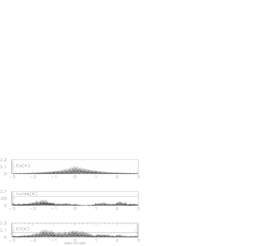
Figure 5: NAUTILUS. The upper figure shows the time behaviour of the applied signal energy with SNR=30, in absence of noise, as in fig.1. The middle figure shows the noise time behaviour at the time this signal was applied. The bottom figure shows the time behaviour of the signal-plus-noise energy. The horizontal line in the middle and lower figures indicates the threshold energy $E_{t}=19.5~{}T_{eff}=65~{}mK$. We see that, in this case, the maximum value of the filtered data occurred 1.422 s before the delta signal was applied (note that in the figure we give the energies, but the signal and noise combine linearly with their amplitudes).

If an additional filter is applied to the data, such as to require i.e. that the detected event behaved in a gaussian way, the signal with SNR=30 is lost, in spite of being a $delta$ signal.

We remark also that the events have energy different from that of the signal. This is shown in tables 2,3 and in fig.6 where we give the distributions of the ratio $\frac{E_{f}}{E_{s}}$ for SNR=30 and SNR=10.

Figure 6: The two upper figures refer to EXPLORER. Distributions of $ES=\frac{E_{f}}{E_{s}}$ for the detected delta signals with SNR=30 (left figure) and SNR=10 (right figure). $E_{f}$ is the energy of the event, $E_{s}$ is the energy of the signal producing the event. The two lower figures refer to NAUTILUS.

Finally we make the following consideration for the case when multiple coincidences with $M$ detectors are searched for. From tables 2 and 3 we deduce that when the signal is near the threshold the efficiency of detection in nearly 50%. This means that for these signals the total efficiency for $M^{pl}$ coincidences is $\sim\frac{1}{2}^{m}$. Since we want an efficiency near unity (because of the very few possible GW signals) we must consider only signals with $SNR$ at least twice the value $SNR_{t}$ of the threshold.

5 Conclusions

We have studied the $events$ generated in a resonant GW detector when excited by GW bursts with $SNR$ near the threshold $SNR_{t}$ used for defining the events. For $SNR=SNR_{t}$ the detection efficiency is nearly $\frac{1}{2}$. The efficiency goes to 100% for $SNR>2~{}SNR_{t}$, and it is still $>10\%$ for $SNR\sim\frac{SNR_{t}}{2}$.

The time of the event might be different from that of the signal, with standard deviation depending on the SNR and on the bandwidth of the experimental apparatus. In this analysis we have applied delta signals at the exact time of the samples. If the delta signals are applied randomly, as in the real case, the efficiency will be smaller and the time dispersion larger.

Delta-like signals can be lost if the requirement to satisfy the theoretical behaviour expected for a delta signal is imposed on the detected events, even for $SNR=30$, as shown in fig.5. This can jeopardize a search looking for very rare gravitational wave signals.

References

- [1] P. Astone et al., Phys. Rev. D. 47, 362 (1993).
- [2] E. Mauceli et al., Phys.Rev. D, 54, 1264 (1996)
- [3] D.G. Blair et al., Phys. Rev. Lett. 74, 1908 (1995).
- [4] P. Astone et al., Astroparticle Physics, 7 (1997) 231-243
- [5] M.Cerdonio et al., First Edoardo Amaldi Conference on Gravitational wave Experiments, pag. 176, Frascati, 14-17 June 1994
- [6] E.Amaldi el al., Astron.Astrophys. 216,325 (1989)
- [7] P.Astone et al, Astroparticle Physics 10 (1999)83-92
- [8] P.Astone et al., Phys.Rev. D,59, 122001 (1999)
- [9] P.Astone, C.Buttiglione,S.Frasca, G.V.Pallottino and G.Pizzella, Il Nuovo Cimento 20,9 (1997)
- [10] S.Boughn et al., Astrophys. J. 261, 119 (1982)
- [11] P.Astone, G.P.Pallottino and G.Pizzella, General Relativity and Gravitation, 30, 105 (1998)
- [12] P.Astone, G.V.Pallottino and G.Pizzella, Class. Quantum Grav. 14 (1997) 2019-2030
- [13] A.Papoulis ”Probability, Random Variables and Stochastic Processes”, McGraw-Hill Book Company (1965), pag 126.
- [14] S.Vitale et al., First Edoardo Amaldi Conference on Gravitational wave Experiments, pag. 220, Frascati, 14-17 June 1994