Atom made from charged elementary black hole

Abstract

It is believed that there may have been a large number of black holes formed in the very early universe. These would have quantised masses. A charged “elementary black hole” (with the minimum possible mass) can capture electrons, protons and other charged particles to form a “black hole atom”. We find the spectrum of such an object with a view to laboratory and astronomical observation of them, and estimate the lifetime of the bound states. There is no limit to the charge of the black hole, which gives us the possibility of observing $Z>137$ bound states and transitions at the lower continuum. Negatively charged black holes can capture protons. For $Z>1$, the orbiting protons will coalesce to form a nucleus (after $\beta$-decay of some protons to neutrons), with a stability curve different to that of free nuclei. In this system there is also the distinct possibility of single quark capture. This leads to the formation of a coloured black hole that plays the role of an extremely heavy quark interacting strongly with the other two quarks. Finally we consider atoms formed with much larger black holes.

I Introduction

Fluctuations in the density of the very early universe led to parts with extremely high density to collapse and form black holes [1, 2, 3]. The density of such objects would be greatly reduced in models of the early universe that include an inflation, but they do not have to disappear entirely. These particles would help explain the mass deficit of the universe.

A black hole is essentially an elementary particle in the sense that it is completely described by a set of quantum numbers and can have no detectable internal structure (the famous “black holes have no hair” theory, see e.g. [4]). Recently it has been demonstrated that the black hole mass is quantised in units of the Planck mass $M_{p}=(\hbar c/G)^{1/2}=1.2\times 10^{19}$ GeV $=2\times 10^{-5}$ g [5] (see also [6, 7, 8, 9]). One intriguing reason for quantisation of black holes comes from a classical formula. The horizon area of Kerr-Newman black holes is

$$A=4\pi\left[\left(M+\sqrt{M^{2}-a^{2}-Q^{2}}\right)^{2}+a^{2}\right]$$ (1)

where $a$ is the angular momentum divided by the mass $M$, and $Q$ is the charge of the black hole. This implies that for a given $a$ and $Q$ there is a minimum mass in order to avoid the singularity of the radical. In ordinary units (the previous equation was written in gravitational units where $\hbar=c=G=1$) one obtains [8]

$$M_{min}=M_{p}\left(Z^{2}\alpha/2+\sqrt{Z^{4}\alpha^{2}/4+J(J+1)}\right)^{1/2},$$ (2)

where $\alpha=e^{2}/\hbar c$; $Ze$ and $J$ are the black hole charge and spin. A black hole with spin can not have mass smaller than 0.93 $M_{p}$. For spinless black holes this equation gives the minimal mass $M_{min}=M_{p}\sqrt{\alpha}=0.085M_{p}$. This classical consideration does not take into account the mass renormalization problem. One can not completely exclude that after the “renormalization” the minimal mass of the charged black hole may be as small as the electron mass.

Such elementary black holes may appear in the very early Universe or as a result of “evaporation” of heavier black holes. We know that black holes radiate with a discrete spectrum in a black body envelope (Hawking radiation[10]), but we cannot say whether a final elementary black hole vanishes completely or what the lifetime of such a process would be. For example, it may not be “easy” for a black hole with $J=1/2$ (or any half-integer spin) to decay since any such decay involves violation of lepton or barion number (e.g. black hole $\rightarrow e^{-}+\gamma$; however, if one views this decay as a “disconnection” of the black hole “inner” universe from our Universe no separate conservation laws for each “universe” should be assumed until they are totally disconnected). We will assume that the elementary black holes do not undergo a final radiation.

The first thing we would like to do is discuss a method to search for elementary black holes. An elementary charged black hole moving through matter at less than a few thousand km s^-1 can capture electrons in the same way as an ordinary atomic nucleus, creating a “black hole atom” [3]. One can search for spectral lines in these systems. Normal nuclei are unstable for very large $Z$, but a black hole can have any charge at all. Furthermore they can have a negative charge, giving rise to whole new types of systems. In fact just about any electrically charged particle can be bound in a black hole atom.

We would like to know whether or not we can do experiments on black holes in a laboratory. Obviously a neutral black hole can simply fall between atoms in the floor of our laboratory and to the centre of the earth, since it is small and the only force acting on it is gravity. However if we have a charged black hole then there is electromagnetic repulsion between atoms and the black hole which may be large enough to keep it in the laboratory. The contact Coulomb force between a neutral atom and the neutral black hole atom (with a charged black hole nucleus) is $\sim e^{2}/a_{0}^{2}\simeq 10^{-7}$ N where $a_{0}$ is the Bohr radius. This equation is just the Coulomb force on the radius of an external electron orbit. Suprisingly, the force due to gravity $M_{p}g$ is also $\sim 10^{-7}$ N for an elementary black hole with the Plank mass. This means that a black hole has large probability to “tunnel” between the atoms and fall through. A lighter spinless black hole may be an exception since the classical equation (2) gives in this case the minimal mass $M_{p}/12$ . The electromagnetic force in this case is an order of magnitude larger than the gravitational force , and such black hole may stay for some time on the surface of the Earth. In this situation it may be reasonable to do both laboratory and astronomical observations. It is easy to calculate the “isotopic” shifts of the black hole lines relative to the usual atomic lines. We discuss the “atomic” spectrum of an elementary black hole in Sec. II with a view to observation of black hole atoms, and verification of their existence. Due to the large mass the black hole spectral lines do not have Doppler broadening and hyperfine structure. This also may help in identification of such lines.

Note that the upper limit on concentration of the black holes follows from the estimate of their mass density. The Plank mass $M_{p}$ is $10^{18}$ times larger than the proton mass. If we assume that the minimal mass of elementary black holes is $M_{p}/12$, and that the dark matter is 100 times heavier than the hydrogen matter and consists of the elementary black holes only, we obtain that the abundance of the elementary black holes in cosmic space does not exceed $10^{-15}$ of the hydrogen abundance (one can compare this with the abundance of uranium $3.10^{-13}$). The limit on the concentration of the elementary black holes can be much stronger if one considers other effects - see, for example, explaination of the deficit of solar neutrinos based on the catalysis of nuclear reactions in the sun by charged black holes [11]. This may practically exclude the possibilty of the observation of the black holes in the spectra of very distant objects. We must rely on the observation of the close objects (like sun spectra) or laboratory data. We should also recall another motivation to search for atoms with superheavy nuclei and shifted atomic lines which is related to so called “strange matter” that have nuclei made from the “normal” (up, down) and strange quarks.

There is a finite probability that an orbiting electron or proton could fall into the central black hole and neutralise it’s charge [3]. This gives a lifetime which is estimated in Sec. III. It is found that the lifetime of low $Z$ electronic atoms is many orders of magnitude larger than the age of the universe, but that it decreases exponentially with $Z$. In fact, we conclude from sections III and IV that primordial black holes would now not have charge greater than about $Z=70$.

We also discuss a few questions which may be of the theoretical interest. In Sec. IV we discuss the K-shell states of black hole atoms for $Z>137$, where there is a well known singularity in the equations. While the single particle solutions of the Dirac equation for high $Z$ has been known for some time, it is worth revisiting these because now we have a physical system where the critical field is realised. We show in this section that the ground state reaches the lower continuum ($E=-mc^{2}$) before $Z=138$ which means that there is no room for negative energy bound states (recall that for $Z=1/\alpha\simeq 137$ the relativistic energy $E\simeq 0$) and hence spontaneous positron emission will occur for all $Z>137$. We also consider a similar problem for a charged scalar particle where the singularity appears for $Z>68$.

If a black hole has a negative charge then it can become a “protonic” atom. The strong force between protons leads to a peculiar ground state characterised by a nucleus orbiting our elementary black hole (Sec. V). It leads to a new stability curve for the captured nucleus, shifted towards more protons (some of the protons still undergo $\beta$-decay to neutrons).

Furthermore we show in Sec. VI that the protonic black hole atom leads to a mechanism by which the black hole can gain a colour charge, by capturing a single quark. This naturally leads to an extension of the “no hair” theorem (which states that any black hole can be characterised by it’s mass, electric charge and spin) to include a colour. Discussion of the solutions of Einstein-Yang-Mills equations for coloured black holes can be found, e.g. in Ref. [12]. We estimate the lifetime of these systems and find that a black hole with colour charge (that may be called a “superheavy quark”) will persist for $10^{7}$ years.

We should note that the single quark capture may be forbidden if the energy of the coloured black hole is higher than that of electrically charged black hole. In this case the lifetime of the protonic black hole can be very long (it contains extra factor $(r_{g}/fm)^{6}\sim 10^{-150}$ where the Planck length $r_{g}=\hbar/M_{p}c=1.6\times 10^{-33}$ cm, $fm=10^{-13}$ cm) since the probabilty of all three quarks to be near black hole horizon is very small. The same argument may be valid for the electron black hole atom if electron is not an elementary particle, i.e. consists of “pre-quarks”. Therefore, one may view lifetime calculations in the present work as the estimates of the minimal lifetimes.

Finally, in Sec. VII, we briefly consider atoms formed when much heavier (with masses $\sim 10^{12}$ kg) black holes capture electrons. The electric charge is shown to neutralise very quickly, but there still remains the possibility of short-lived gravitationally bound systems.

II Black Hole Spectrum

The spectrum of a single electron in a pure central Coulomb potential is given by

$$E=-\frac{mZ^{2}e^{4}}{2\hbar^{2}n^{2}}$$ (3)

where $n$ is the principal quantum number and $Z$ is the charge at the centre. If we have many electrons, then the outer electron energy is usually described by a Rydberg formula

$$E=-\frac{mZ_{a}^{2}e^{4}}{2\hbar^{2}\nu^{2}}$$ (4)

where $\nu$ is an effective principle quantum number, $Z_{a}-1$ is the ion charge ($Z_{a}$ is the charge that the outer electron “sees”; for neutral atom $Z_{a}=1$). To search for black holes we should calculate the level shifts from normal atoms with the same charge. The normal atom spectra thus provides us with a calibration point.

Normal atom spectra are shifted from the “ideal” spectra because of the finite mass and volume of their nuclei. In an elementary black hole atom, however, the mass of the nucleus is practically infinite (over $10^{18}$ proton masses) and it’s volume is zero (around $10^{-60}$ of nuclear volume). Thus we wish to find the energy levels of normal atoms in terms of the ideal (black hole) spectra plus energy shifts due to the finite mass and volume of their nucleus. To improve the accuracy of the calculations one can use experimental data for isotopic shifts in normal atoms.

The theory of isotopic shifts is presented in numerous books (see, e.g. [13]). However, it would be instructive to present some results here with a particular application to the black hole line shifts. The mass shift is given by

$$\Delta E_{m}=E_{A}-E_{\infty}=E_{\infty}.\left(\frac{\mu}{m}-1\right)(1+S)$$ (5)

where $m$ is the electron mass, $\mu=mM/(m+M)$ is the reduced mass, $M$ is the mass of the nucleus, $E_{A}$ is the energy of atomic level, $E_{\infty}$ is the energy of the black hole level (corresponding to infinite $M$) , $S$ is the correction due to the specific mass shift which exists in many-electron atoms. The contribution of the specific shift to the transition frequencies can be calculated or extracted from the experimental data on isotopic shifts (see below).

The volume shift is given by

$$\Delta E_{V}=-e\int\left(\phi-Ze/r\right)\psi^{2}\left(r\right)dV$$ (6)

where $\phi$ is the Coulomb nuclear potential. While this integral is formally extended to all space, it is practically zero outside of the nucleus. For relativistic s-wave electrons

$$\Delta E_{V}\simeq E_{\infty}\frac{6}{\nu}\frac{\gamma+1}{\gamma\left(2\gamma+1\right)\left(2\gamma+3\right)\left[\Gamma\left(2\gamma+1\right)\right]^{2}}\left(2Z\frac{r_{0}}{a_{0}}\right)^{2\gamma}$$ (7)

where $\gamma=\sqrt{1-\left(Z\alpha\right)^{2}}$, $a_{0}=\hbar^{2}/me^{2}$ is the Bohr radius, $r_{0}=1.2A^{1/3}$ is the nuclear radius and $A$ is the mass number of nucleus. To calculate the parameter $\nu$, we simply use eq. 4, since $E$ is the known ionisation energy [14]. The estimates of the normal mass shifts and volume shifts of electron levels in atoms relative to “ideal” black hole atoms are presented in fig. 1 and fig. 2.

FIG. 1.: Mass shifts and s-wave volume shifts in atoms of varying Z (see also fig. 2).

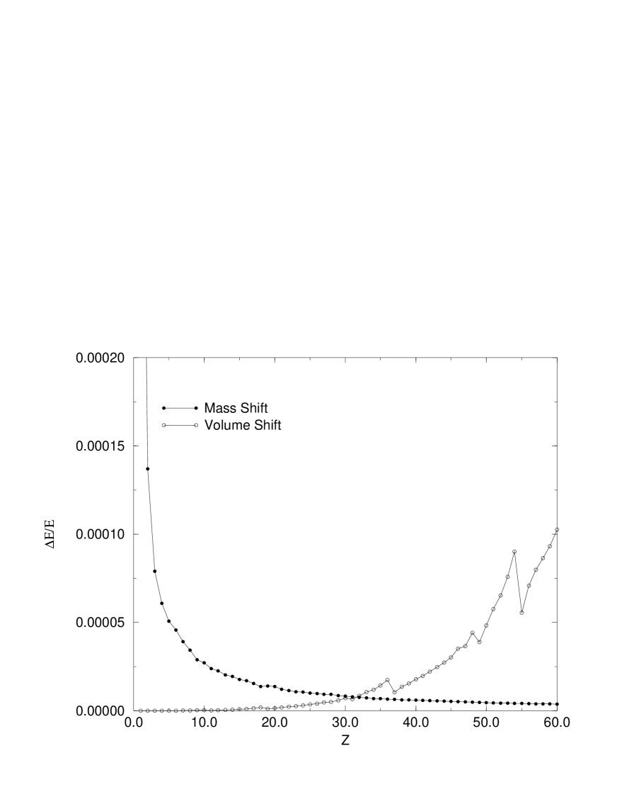
FIG. 2.: Mass shifts and s-wave volume shifts in atoms of varying Z. The effects are equal at about Z = 32.

Consider two examples. In hydrogen the volume shift is very small. We will specifically look at the $2p_{3/2}\rightarrow 1s_{1/2}$ transition. The spectral data is given in [16], which gives for hydrogen and deuterium

$$\omega_{H} = 82259.279{\rm\ cm}^{-1}$$

$$\omega_{D} = 82281.662{\rm\ cm}^{-1}$$

Using the nuclear masses given in [15] we obtain

$$\omega_{\infty}-\omega_{H}=44.801{\rm\ cm}^{-1}$$ (8)

It turns out that this shift is the same for the $2p_{1/2}\rightarrow 1s_{1/2}$ transition.

Now consider Mg II. For magnesium we must include the volume shift. The two isotopes used are ²⁴Mg and ²⁶Mg. From eq. (5) we then obtain

$$\omega_{26}-\omega_{24} = \omega_{\infty}\left(\frac{\mu_{26}}{m}-\frac{\mu_{24}}{m}\right)(1+S)-\Delta E_{V26}+\Delta E_{V24}$$ (9)

$$\omega_{\infty}-\omega_{24} = \omega_{\infty}\left(1-\frac{\mu_{24}}{m}\right)(1+S)+\Delta E_{V24}$$ (10)

Data for the MgII 2796 line (corresponding to the $3p_{3/2}\rightarrow 3s_{1/2}$ transition) have been obtained [17] which give

$$\omega\left({}^{24}{\rm MgII\ }2796\right) = 35760.834\pm 0.004{\rm\ cm}^{-1}$$

$$\Delta\nu\left({}^{26}{\rm Mg}-^{24}{\rm Mg}\right) = 3.050\pm 0.1{\rm\ GHz}$$

$$\omega_{26}-\omega_{24} = 0.1017\pm 0.003{\rm\ cm}^{-1}$$

Now using the formula for volume shift eq. (7) we obtain

$$\Delta E_{V24} = 0.0315{\rm\ cm}^{-1}$$

$$\Delta E_{V26} = 0.0333{\rm\ cm}^{-1}$$

And so eqs. (9,10) give

$$\omega_{\infty}-\omega_{24}=1.378{\rm\ cm}^{-1}$$ (12)

III Lifetime

There is a finite probability that the electrons orbiting a black hole atom enter the black hole. This “direct capture” mechanism leads to a lifetime for the black hole atom. The simplest estimate of the capture probability is given by the product of black hole horizon area $4\pi r_{g}^{2}$ and flux for a particle moving with speed c near this horizon, $j=c\left|\psi_{s}\left(0\right)\right|^{2}$.

$$\frac{1}{\tau}=w\sim\left|\psi_{s}\left(0\right)\right|^{2}4\pi r_{g}^{2}c$$ (13)

Now the K-shell electron is the most likely to be captured. Using relativistic electron wave function from [20] we obtain

$$w\sim\frac{4r_{g}^{2}cZ^{3}}{a_{0}^{3}}\left(\frac{a_{0}}{2Zr_{g}}\right)^{2(1-\gamma)}$$ (14)

A complete picture is given in fig. 3. In all numerical estimates we assume that the mass of the black hole is equal to $M_{p}$. For $Z=1$ this gives lifetime about $10^{22}$ years, for $Z=70$ about the age of the Universe. Thus, elementary black holes formed at the Big Bang with $Z\gtrsim 70$, would have captured electrons in the K-shell, reducing the charge of the black hole. This process would have continued until the present day. Since the lifetime exponentially decreases with $Z$ we would not expect black holes with $Z$ larger than about 70 to exist today.

Note that after the electron has been captured by the black hole, the quantisation rules of the black hole (see Introduction) are no longer obeyed. Thus the black hole must undergo some process to correct itself, such as radiate.

FIG. 3.: Lifetime of K-shell electron as a function of $Z$. On the y-axis is plotted log${}_{10}\left[\mbox{lifetime(sec)}\right]$ because the order of magnitude is of interest.

IV Critically Charged Black Holes

When a black hole forms it inherits the (conserved) quantum numbers of the particles used to form it. This means that most black holes are formed with some non-zero electric charge $Z$. The evaporation process should reduce this charge, however a final charge can still be large. There are some results which are not possible in normal atoms but which may be observed in black hole atoms. For example there are two well known singularities in the single particle solution of the Dirac equation for a Coulomb field, corresponding to particular $Z$ (see e.g. [21]). These single particle solutions are very good approximations for the K-shell (ground state) energy because these electrons are closest to the nucleus and only very lightly screened by the other electrons.

The first singularity occurs when $Z\alpha$ becomes greater than one (Sec. IV A). This singularity is removable when the finite size of the nucleus is taken into account. The second occurs when the ground state energy reaches the lower Dirac sea (Sec. IV B). We call the charge corresponding to this the supercritical charge.

A First critical charge

The solution of the Dirac equation for a Coulomb field $V=-Z\alpha/r^{2}$ has a singularity at $Z\alpha=1$ (or $Z=137.04$). At this point the parameter $\gamma=\sqrt{1-\left(Z\alpha\right)^{2}}$ and the ground state energy $\varepsilon=m\gamma$ become imaginary. In fact nothing much should change when this critical point is passed in a system with a finite nucleus. The energy, $\varepsilon$, becomes negative, but this is entirely allowable.

The physical reason for this singularity is that when $Z\alpha>1$ the particle can “fall to the centre”. The effective potential $U\left(r\right)$, which arises when the Dirac equation is squared and put into a Schrödinger equation - like form, behaves, for a Coulomb field, in a singular manner $U\left(r\right)\approx\left(j\left(j+1\right)-Z^{2}\alpha^{2}\right)r^{-2}$ as $r\rightarrow 0$. This leads, as it does non-relativistically, to all bound state wavefunctions having an infinite number of nodes when $Z\alpha>j+1/2$.

To determine the level energies it is necessary to specify the potential $V\left(r\right)$ and a boundary condition at zero. In any physical system this is obtained by an alteration of the potential at small $r$, due to finite size of the nucleus, or in our case, the black hole. The form of the potential at small $r$ is not important when $Z\alpha<1$ (in fact in our case the black hole should not significantly affect the energy levels even at $Z=137$, since the scale of the cutoff, $r_{0}=10^{-35}$ m, is so small). Yet it does become very important when $Z\alpha>1$.

A lot of interesting physics comes into play when the energy of the K-shell electron goes below zero (but not into the lower continuum). The electrons will have an energy $\varepsilon=-{\rm const}.m$. Therefore it is energetically favourable for the electron to undergo a “ beta decay” into heavier and heavier particles, like a muon, tauon or perhaps some new grand unification particle. This process would be very fast, and in fact it may be possible for this to occur before the particle is captured by the black hole.

Unfortunately in the elementary black hole system none of these effects are realised because the ground state energy falls into the Dirac sea before $Z=138$ (Sec. IV B, see figure 4), and hence there are no negative energy bound states. But the critical value of $Z$ is dependent on the radius of the black hole, and hence it may be possible for bound states with $-m<\varepsilon<0$ to exist in heavier black holes.

B Supercritical charge

If a black hole has a charge larger than some critical value $Z_{c}$ then the K-shell electron energy will reach the lower continuum (the lower Dirac sea) corresponding to energy $\varepsilon=-mc^{2}$. This corresponds to a binding energy of $-2mc^{2}$. This field can spontaneously polarise the vacuum to create an electron - positron pair.

In Appendix A we follow the method outlined by Popov [22] to find that the supercritical charge $Z_{c}=137.29$. Thus when $Z=138$ we are already in the lower continuum, and so we can conclude that there are no K-shell electron bound states with energy $-1<\varepsilon<0$.

When $Z>137$, then, the field can spontaneously polarise the vacuum to create an electron - prositron pair. The electron goes into the K-shell and the positron goes to infinity (in an ordinary nucleus there would be spontaneous emission of two positrons, after which the effective charge of the nucleus decreases by two units, corresponding to filling of the K-shell). In the black hole atom the electron would immediately fall into the black hole, decreasing it’s charge by 1.

This process has a finite lifetime, since the positron must tunnel to infinity to overcome the positive potential it would feel from the black hole. The spontaneous emission of positrons would continue until the charge of the black hole fell below $Z=138$. The ground states with $\varepsilon>0$ also have a finite lifetime, so the charge of the black hole then continues to fall until the charge is neutralised with the lifetimes described in Sec. III.

It is also interesting to consider the binding between black hole and charged scalar particle: Higgs boson, $\pi$-meson, etc. For a scalar particle, the Klein-Gordon equation in the Coulomb field has a singularity at $Z\alpha=1/2$ (or $Z=68.5$). After this we must take into account the finite size of the nucleus. We wish to know at which point the energy reaches the lower continuum, to see whether there are any bound states with negative energy (in much the same fashion as was done for the electron case).

The calculation to find the critical charge in the case of the scalar particle is done in Appendix B, again following the method of Popov [22]. It is found that the bound state energy of the lowest shell equals $-mc^{2}$ at $Z_{c}=69.001$. Due to uncertainty in the size and boundary condition of the black hole we cannot, from these results, tell if there is a $Z=69$ bound state or not. Anyway, it would be a very short-lived state.

In a case of a finite-size particle like $\pi$-meson the low-$Z$ Klein-Gordon equation may be treated in a similar fashion to the “finite-size nucleus” problem with the radius of $\pi$-meson instead of nuclear radius. However, accurate high-$Z$ results may be obtained only by solution of the three-body problem and depends on the strong interactions between the quarks. For example, one of the quarks can be rapidly captured by a black hole and they can form a “superheavy quark” interacting with a remaining quark - see next section devoted to a protonic black hole.

FIG. 4.: K-shell electron and scalar particle energy as a function of Z. The electron energy reaches zero at $Z\alpha=1$ or $Z=137.036$. In the case where the nucleus is an elementary black hole, the energy reaches the Dirac sea ($\varepsilon/m=-1$) at $Z_{c}=137.29$, implying that there are no negative energy bound states. In the scalar particle case the energy reaches the Dirac sea very close to $Z_{c}=69$, so we cannot easily tell whether there is a bound state with negative energy or not.

V Protonic Black Hole Atoms

If a black hole has a negative charge, then it can capture positively charged particles including protons and alpha particles. At first glance, one might think that this would form a “protonic black hole atom”, something akin to usual atoms, but with orbiting protons instead of electrons. But in fact the physics of this system is quite different.

A Ground state

Consider a protonic black hole. Because of the strong nuclear force, the ground state of this system would consist of a “nucleus” of protons (some of which may decay into neutrons) orbiting a black hole. For a singly charged black hole, there would simply be a single bound proton and nothing very exciting occurs (until it decays - see Sec. VI).

It is known that for two nucleons there are no bound isotopic triplet states. This means that in a system of two protons orbiting a black hole of charge $Z=-2$, one of the protons should decay via the weak interaction as

$$p^{+}\rightarrow n+e^{+}+\nu$$ (15)

and thus acheive a stable deuterium nucleus configuration. However this is not the end of the story. The positron would be emitted with a large kinetic energy and so it would only be weakly bound if at all. Thus the system will still have an effective charge of $-1$, which can attract another proton. This would join with the deuterium nucleus and form a ³He nucleus.

Also it is concievable that the doubly charged black hole could pick up an extra neutron, if a sufficiently slow one chanced by the orbiting nucleus. Then the tritium nucleus would be formed. This would certainly be unstable, as it is usually, and decay to ³He.

We now have the idea that the negatively charged black hole can have a nucleus orbiting it, having a certain number of neutrons and protons which follow the nuclear stability curve. But we have not considered the effect of the Coulomb field on this nucleus. The binding energy of the nucleus will decrease when protons decay to neutrons because the neutrons are not charged. This may provide enough energy in some cases to form a bound state with an unusually high number of protons. So the stability curve is effectively pushed towards the proton side.

B Lifetime

The lifetime found from eq. 14 is proportional to $m^{-2\gamma-1}$, where $m$ is the mass of the orbiting particle. This means that a single proton orbiting around an elementary particle of charge $Z=1$ has a decay probability $\left(m_{p}/m_{e}\right)^{3}=1836^{3}$ times larger, leading to a lifetime of $\tau=3\times 10^{12}$ years.

But the mass of our particle will be that of the orbiting nucleus, which must in turn follow the new stability curve for a nucleus orbiting a black hole (Sec. V A). Thus the lifetimes will decrease even faster than they do in the electron case because the entire nucleus mass is of importance, not the mass of just one proton. However, if we consider black hole with only one proton the lifetime is equal to the age of the Universe for $Z=5$.

There is an additional complication to the lifetime, considered in Section VI.

VI Colour Charge in Black Holes

We have established in Section V that negatively charged black holes can have orbiting protons. We even estimated the probability that the bound protons fall into the black hole. But we did not consider that protons are not elementary particles, but are made up of three quarks, each with a different colour charge. This means that due to the extremely small size of the elementary black hole, it is not the entire proton which is captured, but a single quark!

The black hole then obtains the colour of the quark it captured, and becomes a “superheavy quark”. This would form a strongly bound state with the remaining two quarks of the original proton. While the other two quarks will eventually fall into the black hole, this will happen with a finite lifetime $\tau\sim 10^{7}$ years. Here we assumed that the quark wave function in the proton has the radius $R\sim 0.5$ fm and $\psi(0)^{2}=1/(4\pi R^{3}/3$).

VII Heavier Black Holes

Let us discuss briefly non-elementary black holes. Because the density fluctuations in the early universe would have occurred on all scales [2], there may conceivably have been black holes formed with much larger masses. The smaller ones of these would have evaporated into elementary black holes. The minimal mass of a black hole that would not have evaporated entirely by now is $M\sim 5\times 10^{11}$ kg [2]. In this chapter we will consider black holes of mass $M\sim 10^{12}$ kg. Such an object has a radius of 1.5 fm.

These objects are interesting to study because at this mass they have gravitational fields comparable to the electric field, as well as sizes comparable to that of ordinary nuclei. Unfortunately there is another complication in determining orbits - the constant flux of Hawking radiation being emitted will interfere with any particle orbits.

Consider a singly charged black hole. Neglecting the gravitational potential and using equation 14 for capture probability with a new Schwarzschild radius of 1.5 fm, we obtain the lifetime

$\displaystyle\tau_{\rm Coulomb}=5\times 10^{-11}{\rm\ sec}$

Obviously increasing the charge makes this smaller still, as does including the gravity term. Thus we can conclude from this, and the fact that if it was charged, evaporation would favour neutralisation of charge, that any charge of the black hole would have been neutralised by now.

Having concluded that there would be no electric charge on black hole atoms, we turn our attention to gravitational atoms. These would consist of particles (we will confine ourselves to electrons, but any particle would do) orbiting heavy black holes of the mass discussed. The potential is

$$U_{\rm grav}=-\frac{GMm}{r}=-\frac{g}{r}$$ (16)

In relativistic units, $g=1/520$ for electrons. The radius of the ground state for such a system is approximately $a=1/gm=2\times 10^{-11}$ m $=0.2$ nm. This does not take into account the continual radiation of the black hole which can interact with the particles and may potentially destroy the bound states.

VIII Conclusion

We have seen that elementary black holes with charge can capture electrons and form bound states similar to those of an ordinary atom. The electronic spectra of these black hole atoms can be searched.

The electrons orbiting a black hole can fall into it. This “direct capture” leads to a finite lifetime for black hole atoms. This was found to be many times the age of the universe for black holes with small charges, but decreasing exponentially with increasing Z. From these calculations we concluded that primordial black holes would today have charges no larger than $Z\approx 70$.

The black hole atoms may give rise to new physical phenomena. When $Z>137$ ($Z>68$ for scalar particles) we have a physical realisation of the much theorised supercritical Coulomb fields, where the single particle K-shell energy becomes negative. We found that these energies immediately drop into the lower continuum $\varepsilon<-mc^{2}$. Although the ground state falls into the Dirac sea at $Z\alpha=1.002$, the upper states ($p_{3/2}$, $d$, etc.) do not until after $Z\alpha=\left|\kappa\right|$ (see [21]). Therefore it remains as an interesting question whether there are any states with negative energy (including $mc^{2}\,$) in the upper bound states. If there are, then there is still the possibility of beta decay of electrons to muons, tauons, and so on.

We also discussed protonic black hole atoms which are formed with negatively charged elementary black holes. The ground state of such systems is a nucleus orbiting a black hole, with the nuclear stability curve pushed towards the proton side. Because protons are not elementary particles, the black holes would capture just one of the quarks of the proton (or of any constituent nucleon in the orbiting nucleus). This leads to a black hole with a colour charge. The lifetime of this “superheavy quark” was found to be about $10^{7}$ years.

Finally we briefly considered much heavier black holes (with masses of $\sim 10^{12}$ kg) and found that their charge is neutralised very rapidly. There remains the possibility of gravitational atoms. However, because of Hawking radiation and the capture of the electron, such atoms may be very short-lived.

We are grateful to M.Yu.Kuchiev for valuable discussion. This work was supported by the Australian Research Concil.

A Supercritical charge - electron case

Here we proceed to find the supercritical $Z$, following the method outlined by Popov [22]. To find $Z_{c}$ we need to solve the Dirac equation for $\varepsilon=-1$ (we use relativistic units $\hbar=c=m=1$). We write the potential as

$$V\left(r\right)=\{\begin{array}[]{l}-\xi/r\ \ ,\ r>r_{g}\\ -\xi/r_{g}\ ,\ 0<r<r_{g}\end{array}$$ (A1)

where $\xi=Z\alpha$. This assumes that the wavefunction can extend inside the black hole, and that the charge of the black hole is concentrated entirely on the surface of it. The Dirac equation can be expressed [18]

$$\frac{dF}{dr} = -\frac{\kappa}{r}F+\left(1+\varepsilon-V\right)G$$ (A2)

$$\frac{dG}{dr} = \left(1-\varepsilon+V\right)F+\frac{\kappa}{r}G$$ (A3)

where $F\left(r\right)=rf\left(r\right)$ and $G\left(r\right)=rg\left(r\right)$, with $f$ and $g$ the radial wavefunctions, $-\kappa$ is the eigenvalue of the operator $K=\beta\left(L\cdot\sigma+1\right)$, conserved in a spherically symmetric field. For K-shell electrons, $\kappa=-1$.

We eliminate $G$ from eq. A3 to obtain the second order differential equation

$$F^{\prime\prime}+\frac{V^{\prime}}{1+\varepsilon-V}\left(F^{\prime}+\frac{\kappa}{r}F\right)+\left[\left(\varepsilon-V\right)^{2}-1-\frac{\kappa\left(\kappa+1\right)}{r^{2}}\right]F=0$$ (A4)

The wavefunction outside the black hole can be obtained from this, setting $\varepsilon=-1$ and $V=-\xi/r$ where $\xi$ now becomes it’s critical value when the bound state reaches the lower continuum, $\xi_{c}$,

$$r^{2}F^{\prime\prime}+rF^{\prime}+\left(\xi^{2}-\kappa^{2}-2\xi r\right)F=0$$ (A5)

Transforming this equation by $x=\sqrt{8\xi r}$ we obtain the Bessel equation

$$x^{2}F^{\prime\prime}+xF^{\prime}-\left(x^{2}-\nu^{2}\right)F=0$$ (A6)

with $\nu=2\sqrt{\xi^{2}-\kappa^{2}}$. This leads to the solution (for $\kappa=-1$ and $\xi>1$)

$$F={\rm constant\ }K_{i\nu}\left(x\right)={\rm constant\ }K_{i\nu}\left(\sqrt{8\xi r}\right)$$ (A7)

where $K_{i\nu}\left(x\right)$ is the MacDonald function of imaginary order (a Bessel function of the second kind). The second independent solution $I_{i\nu}\left(\sqrt{8\xi r}\right)$ is unacceptable because of it’s growth at infinity.

Now we must choose a boundary condition at $r=r_{g}$, hence specifying completely the wavefunction $F$ and allowing us to find $\xi_{c}$. For the potential considered in eq. A1, we equate the logarithmic derivatives of the wavefunctions inside and outside the black hole (for details see [22]) and obtain the transcendental equation

$$xK^{\prime}_{i\nu}\left(x\right)=2\xi\cot\xi K_{i\nu}\left(x\right)$$ (A8)

Solving this for $r_{g}=1.6\times 10^{-35}{\rm\ m}=4\times 10^{-23}$ in the relativistic units used we obtain $\xi=Z_{c}\alpha=1.00187$ corresponding to a critical charge

$$Z_{c}=137.29$$ (A9)

Thus we conclude that there are no (K-shell) bound states with energy $-1<\varepsilon<0$ because when $Z=138$ we are already in the lower Dirac sea.

One may think that the boundary condition chosen is somewhat artificial, but in fact the actual boundary condition chosen is not important compared to the scale of $r_{g}$. Consider, for example a very general (and incomplete) boundary condition $K_{i\nu}\left(\sqrt{8\xi r_{g}}\right)={\rm constant}$. The constant should necessarily be positive because the ground state should have no nodes. The maximum value of $\xi$ will be realised when a node does exist at the boundary. So let’s try $K_{i\nu}\left(\sqrt{8\xi r_{g}}\right)=0$. This gives us a value of $\xi_{c}=1.00199$ corresponding to $Z_{c}=137.31$. So our conclusion that no negative energy bound states exist is valid.

B Supercritical charge - scalar case

We can discuss the case of a point-like scalar particle in a Coulomb field in an analagous manner to the electron case [22]. Firstly, we must solve the Klein-Gordon equation, outside the nucleus

$$\varphi_{l}^{\prime\prime}+\left(\varepsilon^{2}-1+\frac{2\varepsilon\xi}{r}+\frac{\xi^{2}-l\left(l+1\right)}{r^{2}}\right)\varphi_{l}=0$$ (B1)

We can solve this in it’s present form, but it is easier if we set $\varepsilon=-1$ immediately, since we are interested in finding $\xi_{c}$, where the K-shell energy meets the lower continuum. The wavefunction in this case has the form

$$\varphi_{l}\left(r\right) = \sqrt{r}\,K_{i\mu}\left(\sqrt{8\xi R}\right)$$ (B2)

$$\mu = 2\sqrt{\xi^{2}-\left(l+\frac{1}{2}\right)^{2}}$$ (B3)

If we again use the cut-off potential for $V\left(r\right)$ then we obtain for $\xi_{c}$ the transcendental equation (for the lowest level $n=1$, $l=0$)

$$xK^{\prime}_{i\nu}\left(x\right) = \left(2\beta\,{\rm cot}\,\beta-1\right)K_{i\nu}\left(x\right)$$ (B4)

$$\nu = \sqrt{4\xi^{2}-1}$$ (B5)

$$\beta = \sqrt{\xi\left(\xi-2R\right)}$$ (B6)

$$x = \sqrt{8\xi R}$$ (B7)

Solving this numerically we obtain that $\xi_{c}=0.50353$ which means that the energy of the scalar particle reaches the Dirac sea at $Z_{c}=69.001$. Due to uncertainties in the size and boundary condition of the black hole, we cannot tell if there is a bound state with negative energy at $Z=69$.

REFERENCES

- [1] Ya.B.Zel’dovich, I.D.Novikov, Astron. Zhurn. 43, 758 (1966).
- [2] C.W.Misner, in Batelle Rencontres in Mathematics and Physics, ed. De Witt and B.Wheeler, (1968).
- [3] S.Hawking, Mon. Not. R. astr. Soc. 152, 75-78, (1971).
- [4] W.Israel, in 300 years of Gravitation, eds. S.W.Hawking and W.Israel (Cambridge University Press, 1987).
- [5] J.D.Bekenstein and V.F.Mukhanov, Phys. Lett. B. 360,1-2 (1995).
- [6] J.D.Bekenstein, Lett. Nuovo Cimento 11, 467 (1974).
- [7] V.Mukhanov, JETP Letters 44, 63 (1986).
- [8] P.Mazur, Gen. Rel. Grav. 19, 1173 (1987).
- [9] I.B.Kriplovich, Phys. Lett. B. 431, 19-21 (1998).
- [10] S.W.Hawking, Nature 248 , 30 (1974); Commun. Math. 43, 199 (1975).
- [11] E.M.Drobyshevski, Mon. Not. R. Astron. Soc. 282,211 (1996).
- [12] D.Maison, Proc. 8th M. Grossman Meeting on General Relativity. Ed. Tsvi Piran, series ed. Remo Ruffini (World Scientific, 1999), p. 530.
- [13] I.I.Sobel’man, Introduction to Theory of Atomic Spectra, (Moscow, 1977).
- [14] G.Aylward and T.Findlay, S.I. Chemical Data, (Wiley, 1994).
- [15] C.M.Lederer and V.S.Shirley, Table of Isotopes, (Wiley, 1978)
- [16] Selected Tables of Atomic Spectra, NSRDS-NBS 3, Section 6 (U.S. Dept. of Commerce, 1972).
- [17] R.E.Drullinger, D.J.Wineland and J.C.Bergquist, Appl. Phys. 22, 265, (1980).
- [18] V.B.Berestetskii, E.M.Lifshitz, L.P.Pitaevsky, Relativistic Quantum Theory, (L.D.Landau and E.M.Lifshitz, Theoretical Physics,v. 4), (Pergamon Press Ltd, 1971).
- [19] L.D.Landau and E.M.Lifshitz, The Classical Theory of Fields, (Pergamon Press Ltd, 1965).
- [20] J.D.Bjorken, S.D.Drell, Relativistic Quantum Mechanics, v.1 (McGraw - Hill, 1964).
- [21] Ya.B.Zel’dovich and V.S.Popov, Sov. Phys. Uspekhi 14, 6, 673, (1972).
- [22] V.S.Popov, Sov. J. Nucl. Phys. 12, 2, 235 (1971).