Iterated function systems and permutation representations of the Cuntz algebra

Abstract.

We study a class of representations of the Cuntz algebras $\mathcal{O}_{N}$, $N=2,3,\dots$, acting on $L^{2}\left(\mathbb{T}\right)$ where $\mathbb{T}=\mathbb{R}\diagup 2\pi\mathbb{Z}$. The representations arise in wavelet theory, but are of independent interest. We find and describe the decomposition into irreducibles, and show how the $\mathcal{O}_{N}$-irreducibles decompose when restricted to the subalgebra $\mathop{\rm UHF}\nolimits_{N}\subset\mathcal{O}_{N}$ of gauge-invariant elements; and we show that the whole structure is accounted for by arithmetic and combinatorial properties of the integers $\mathbb{Z}$. We have general results on a class of representations of $\mathcal{O}_{N}$ on Hilbert space $\mathcal{H}$ such that the generators $S_{i}$ as operators permute the elements in some orthonormal basis for $\mathcal{H}$. We then use this to extend our results from $L^{2}\left(\mathbb{T}\right)$ to $L^{2}\left(\mathbb{T}^{d}\right)$, $d>1$; even to $L^{2}\left(\mathbf{T}\right)$ where $\mathbf{T}$ is some fractal version of the torus which carries more of the algebraic information encoded in our representations.

1. Introduction

Let $\mathcal{H}$ be the Hilbert space $L^{2}\left(\mathbb{T}\right)$, $\mathbb{T}=\mathbb{R}\diagup 2\pi\mathbb{Z}$ the torus, and let $\left\{z^{n}\right\}_{n=-\infty}^{\infty}$ be the usual orthonormal basis of Fourier analysis: the convention is $z=e^{it}$ and $z^{n}=e^{itn}$, $t\in\mathbb{R}$, $n\in\mathbb{Z}$; and the Haar measure on $\mathbb{T}$ will be normalized. The following representations of $\mathcal{O}_{N}$ (the Cuntz algebra of index $N$, [Cun77]) arise in the study of filter-banks in wavelet theory; see, e.g., [Dau], [CoRy], [DDL], [Jor95], [DaLa], [JoPe96], and [JoPe94]. Let functions $\left\{m_{i}\right\}_{i=0}^{N-1}\subset L^{\infty}\left(\mathbb{T}\right)$ be given such that the corresponding $N\times N$ matrix

(1.1) $$\left(m_{k}\left(e^{i\frac{2\pi l}{N}}z\right)\right)_{k,l=0}^{N-1}$$

is unitary. If, for example, $N=2$, the condition is unitarity of $\smash{\left(\begin{smallmatrix}m_{0}\left(z\right)&m_{0}\left(-z\right)\\ m_{1}\left(z\right)&m_{1}\left(-z\right)\end{smallmatrix}\right)}$ $(\mathrm{a.a.}\,z\in\mathbb{T})$. If $m_{0}\in L^{\infty}\left(\mathbb{T}\right)$ is given, subject to the condition

(1.2) $$\left|m_{0}\left(z\right)\right|^{2}+\left|m_{0}\left(-z\right)\right|^{2}=1\text{\quad}\left(\mathrm{a.a.}\,z\in\mathbb{T}\right)\text{,}$$

then setting $m_{1}\left(z\right)=z\overline{m_{0}\left(-z\right)}$, the unitarity property follows. Similarly, if $f\in L^{\infty}\left(\mathbb{T}\right)$ is unimodular, i.e., $\left|f\left(z\right)\right|=1$ $\mathrm{a.a.}\,z\in\mathbb{T}$, then

(1.3) $$m_{1}^{f}\left(z\right):=zf\left(z^{2}\right)\overline{m_{0}\left(-z\right)}$$

is an admissible choice, and, in fact, conversely, any $m_{1}$ has this form; see [Dau].

The announced representation of $\mathcal{O}_{N}$ is defined from the functions $m_{i}$ as follows:

$$S_{i}\xi\left(z\right)=N^{\frac{1}{2}}m_{i}\left(z\right)\xi\left(z^{N}\right)$$

for $i\in\mathbb{Z}_{N}=\mathbb{Z}\diagup N\mathbb{Z}$, $\xi\in L^{2}\left(\mathbb{T}\right)$, and $z\in\mathbb{T}$. These representations were introduced in [Jor95]. The corresponding adjoint operators $S_{i}^{*}$ occur in more general contexts (although not as representations) in Ruelle’s theory [Rue94] under the name “transfer operators”.

Our analysis of the trigonometric basis $\left\{z^{n}\right\}_{n\in\mathbb{Z}}$ (and the corresponding multi-variable case) is based on another viewpoint which is more special in some respects and more general in others. It is based on iterated function systems (i.f.s.); and we refer to [Mau], [JoPe95], and [Str95] for details on previous work. The theory of i.f.s. divides itself into: (i) the fractals (iteration of “small” scales), and (ii) the “large” discrete systems. Our emphasis here will be (ii), and Strichartz [Str95] has suggested the name “fractals in the large”, or reverse iterated function systems (r.i.f.s.) for the latter viewpoint. But let us call attention to the duality between (i) and (ii) (studied for example in [Str95] and [JoPe95]), in the sense that (i) and (ii) serve as the two sides of Fourier duality. This viewpoint is inspired by classical Pontrjagin duality (see, e.g., [BraRo] and [HRW]), but the new feature here is that neither side of the (i)–(ii) setting in its fine structure alone admits group duality. Instead we base our analysis on an associated discrete dynamical system. This system in turn is tailored to the Cuntz algebra $\mathcal{O}_{N}$.

The simplest examples, for $N=2$, arise as follows: let $s$ be an odd integer, and let the matrix be $2^{-\frac{1}{2}}\begin{pmatrix}1&1\\ z^{s}&-z^{s}\end{pmatrix}$. Then

(1.4) $$\left(S_{0}\xi\right)\left(z\right) =\xi\left(z^{2}\right)\text{,}$$

$$\left(S_{1}\xi\right)\left(z\right) =z^{s}\xi\left(z^{2}\right)\text{,\quad}\forall\xi\in L^{2}\left(\mathbb{T}\right)\text{, }\mathrm{a.a.}\,z\in\mathbb{T}\text{,}$$

and we note that

(1.5) $$\begin{split}&S_{i}^{*}S_{j}=\delta_{ij}\hbox{\small 1\kern-3.3pt\normalsize 1}\text{\quad and}\\ &\sum_{i=0}^{1}S_{i}S_{i}^{*}=\hbox{\small 1\kern-3.3pt\normalsize 1}\text{,}\end{split}$$

where 11 is the identity operator in $\mathcal{H}=L^{2}\left(\mathbb{T}\right)$.

Similarly, if $N\in\left\{2,3,\dots\right\}$, and $D=\left\{s_{i}\right\}_{i=0}^{N-1}\subset\mathbb{Z}$ is a set of integers such that any two distinct members are mutually incongruent modulo $N$, then the operators

(1.6) $$\left(S_{i}\xi\right)\left(z\right)=z^{s_{i}}\xi\left(z^{N}\right)$$

(for $\xi\in L^{2}\left(\mathbb{T}\right)$), satisfy the Cuntz relations

(1.7) $$\begin{split}&S_{i}^{*}S_{j}=\delta_{ij}\hbox{\small 1\kern-3.3pt\normalsize 1}\text{\quad and}\\ &\sum_{i=0}^{\hbox to0.0pt{\hss$\scriptstyle N-1$ \hss}}S_{i}S_{i}^{*}=\hbox{\small 1\kern-3.3pt\normalsize 1}\text{.}\end{split}$$

Recall that the Cuntz algebra $\mathcal{O}_{N}$ is the $C^{*}$-algebra generated by $S_{0},\dots,S_{N-1}$ satisfying (1.7). This algebra is simple [Cun77]. Every system of operators $\left\{S_{i}\right\}$ on a Hilbert space $\mathcal{H}$, subject to these same relations, then determines a representation $\pi$ of $\mathcal{O}_{N}$ on $\mathcal{H}$, i.e., $\pi\in\mathop{\rm Rep}\left(\mathcal{O}_{N},\mathcal{H}\right)$. (See, e.g., [EvKa, Section 2.8] and [PoSt] for basic facts on representation theory.)

In Section 2 we will embed the representation defined in (1.6) into a much more general class of representations coming from certain iterated function systems, called permutative, multiplicity-free representations, and one of the main results of this paper is the embedding of all these into a universal permutative, multiplicity-free representation; see Corollary 7.1. This embedding is in terms of an embedding of our iterated function systems into a certain “coding space” which is a variant of a dynamical systems tool used also in [Jor95], [Pri], [PoPr], [BreJo], [EHK] and more generally in [Rue94]. Another special way of obtaining such representations is to replace $L^{2}\left(\mathbb{T}\right)$ with $L^{2}\left(\mathbb{T}^{\nu}\right)$, and fix a matrix $\mathbf{N}$ with integer coefficients such that $\left|\det\left(\mathbf{N}\right)\right|=N$. Then choose a set $D=\left\{d_{1},\dots,d_{N}\right\}$ of points in $\mathbb{Z}^{\nu}$ which are incongruent modulo $\mathbf{N}\mathbb{Z}^{\nu}$, i.e., $d_{i}-d_{j}\notin\mathbf{N}\mathbb{Z}^{\nu}$ for $i\neq j$. As in elementary arithmetic, one proves that the quotient mapping $\mathbb{Z}^{\nu}\rightarrow\mathbb{Z}^{\nu}\diagup\mathbf{N}\mathbb{Z}^{\nu}$ is $1$–$1$ when restricted to $D$, and if $d_{i}$ are incongruent modulo $\mathbf{N}\mathbb{Z}^{\nu}$ then $d_{i}+\mathbf{N}l_{i}$ are incongruent modulo $\mathbf{N}\mathbb{Z}^{\nu}$ for any choice of $l_{i}\in\mathbb{Z}^{\nu}$, and these vectors constitute the most general choice for $D$. The associated representation of $\mathcal{O}_{N}$ is given by

(1.8) $$\left(S_{i}\xi\right)\left(z\right)=z^{d_{i}}\xi\left(z^{\mathbf{N}}\right)$$

where we define

$$z =\left(z_{1},\dots,z_{\nu}\right)\in\mathbb{T}^{\nu}$$

$$z^{d_{i}} =z_{1}^{d_{i1}}z_{2}^{d_{i2}}\cdots z_{\nu}^{d_{i\nu}}$$

$$z^{\mathbf{N}} =\left(z_{1}^{n_{11}}\cdots z_{\nu}^{n_{1\nu}},z_{1}^{n_{21}}\cdots z_{\nu}^{n_{2\nu}},\dots,z_{1}^{n_{\nu 1}}\cdots z_{\nu}^{n_{\nu\nu}}\right)$$

if $\mathbf{N}=\left(n_{ij}\right)_{i,j=1}^{\nu}$. These types of representations have been considered in [JoPe96], [Ban91], [Str94]. To make these representations multiplicity-free, one needs the extra assumption

$$\bigcap_{k}\mathbf{N}^{k}\mathbb{Z}^{\nu}=0$$

on $\mathbf{N}$; see (3.8). In analyzing the properties of these representations, the dynamical system defined by a certain $N$ to $1$ map $R:\mathbb{Z}^{\nu}\rightarrow\mathbb{Z}^{\nu}$ will play a dominant role. In these cases, $R$ is defined by the requirement

(1.9) $$R\left(d_{i}+\mathbf{N}x\right)=x\text{,}$$

and since (as we show) $R$ behaves like $\mathbf{N}^{-1}$ on a large scale, both $\mathbf{N}$ and $D$ (up to permutation of the indices) can be recovered from $R$, as a consequence of the fact that $R$ behaves like $\mathbf{N}^{-1}$ at large distances. See Scholium 2.5, the discussion around (3.7)–(3.8), Proposition 3.12, and Subsection 9.2.

There are some similarities and some differences between the analysis of the monomial representations (1.8) in one dimension (i.e., (1.6)), and in higher dimensions. We study both cases below: Section 8 ($\nu=1$), and Section 9 ($\nu>1$). Our analysis in Section 8 in the case $N=2$ is based partly on factorization of the Mersenne numbers, whereas the higher-dimensional cases (Section 9) involve the geometry of a set $\mathbf{T}$ of generalized fractions constructed from a given pair $\left(\mathbf{N},D\right)$ in $\nu$ dimensions where the matrix $\mathbf{N}$ is as described, and $D$ represents generalized “digits”, i.e. the vector version of such. See (3.11)–(3.12) for the precise definitions. One of the conclusions coming out of our analysis in Sections 8–9 is that there are infinite families of non-isomorphic examples. See [BaGe] and [Gel] on the isomorphism problem for the “reptiles” based on $\left(\mathbf{N},D\right)$ systems. Some of the properties of these reptiles can be understood from our study of periodic points of the transformation $R$ from (1.9), and also from the question of which rank-$\nu$ lattices $\mathbb{L\kern 0.5pt}$ make $\mathbf{T}$ tile $\mathbb{R}^{\nu}$. We also establish in Section 9 a connection between the last two, i.e., periodic points and lattices. Another variation of the construction in the previous paragraph is to replace $\ell^{2}\left(\mathbb{Z}^{\nu}\right)$ with the Hilbert space spanned by the monomials $z^{n}$ where $n$ is specified to lie in a certain subset $S$ of $\mathbb{Z}^{\nu}$, and we define the operators $S_{i}$ by the same formula as before, i.e., (1.8), but with the function $\xi$ restricted to lie in the corresponding closed subspace $\left({}\subset L^{2}\left(\mathbb{T}^{\nu}\right)\right)$. Instead of assuming the elements of $D$ be mutually incongruent $\bmod{\,\mathbf{N}\mathbb{Z}^{\nu}}$, we now merely need to assume that $S=\bigcup_{i=1}^{N}\left(d_{i}+\mathbf{N}S\right)$, and $\left(d_{i}+\mathbf{N}S\right)\cap\left(d_{j}+\mathbf{N}S\right)=\emptyset$ for $i\neq j$. This structure occurs in some dynamical systems considered by [Ken], [Odl], and [LaWa2], and is treated in detail in Remark 3.14.

Let $\mathcal{B}\left(\mathcal{H}\right)$ denote the $C^{*}$-algebra of all bounded operators on the Hilbert space $\mathcal{H}$. In [Arv], [Lac], and [BJP] it was noted that the study of the endomorphisms of $\mathcal{B}\left(\mathcal{H}\right)$, i.e., $\mathop{\rm End}\left(\mathcal{B}\left(\mathcal{H}\right)\right)$, is equivalent to that of $\mathop{\rm Rep}\left(\mathcal{O}_{N},\mathcal{H}\right)$. If $S_{i}$ satisfy (1.7), then an endomorphism $\alpha$ is defined by

(1.10) $$\alpha\left(A\right)=\sum_{i=0}^{N-1}S_{i}AS_{i}^{*}\text{,\quad}A\in\mathcal{B}\left(\mathcal{H}\right)\text{;}$$

and, conversely, every $\alpha\in\mathop{\rm End}\left(\mathcal{B}\left(\mathcal{H}\right)\right)$ is of this form.

Consider the automorphism group (“gauge group”) of $\mathcal{O}_{N}$, denoted by $\left(\gamma_{z}\right)_{z\in\mathbb{T}}$, which is determined by $\gamma_{z}\left(S_{i}\right)=zS_{i}$, $z\in\mathbb{T}$. The subalgebra $\mathop{\rm UHF}\nolimits_{N}$ of gauge-invariant elements is

(1.11) $$\mathop{\rm UHF}\nolimits_{N}:=\left\{a\in\mathcal{O}_{N}:\gamma_{z}\left(a\right)=a,\;\forall z\in\mathbb{T}\right\}\text{.}$$

It is a $\mathop{\rm UHF}$ algebra of Glimm type $\mathcal{M}_{N^{\infty}}$ (see, e.g., [Cun77], [BraRo], [BJP], and [BraJo]). For general representations $\pi\in\mathop{\rm Rep}\left(\mathcal{O}_{N},\mathcal{H}\right)$, the corresponding restrictions $\pi|_{\mathop{\rm UHF}\nolimits_{N}}$ have been studied in, e.g., [BEEK] and [Pow88].

In those studies, the case when $\pi\left(\mathop{\rm UHF}\nolimits_{N}\right)$ is weakly*-dense in $\pi\left(\mathcal{O}_{N}\right)$ is predominant. However, in the present examples this weak*-density does not hold. We will show that, in the $D$-examples, the $\mathcal{O}_{N}$-irreducibles, when restricted to $\mathop{\rm UHF}\nolimits_{N}$, break up as finite orthogonal sums of mutually inequivalent $\mathop{\rm UHF}\nolimits_{N}$-irreducibles. Hence, we get the $C^{*}$-algebra version of what in group theory is called “Gelfand pairs”; see, e.g., [BeRa] and [BJR].

In group theory, the occurrence of Gelfand pairs appears to be rare, and when it happens, the representation theory appears to account for the underlying structure of the groups in question. Let $G$ be a group with a subgroup $K$, and let $\pi$ denote some unitary representation of $G$ on a Hilbert space. The restriction of $\pi$ to $K$ will be denoted $\pi|_{K}$. We say that $\left(G,K\right)$ is a Gelfand pair if the irreducibles $\pi$ of $G$ are multiplicity-free when restricted to $K$. Typically, we may not know all the (equivalence classes of) irreducible representations of $G$, and the definition then applies instead to a suitably restricted family of irreducibles of $G$.

The analogy to the present setting is clear from this: we have $\mathop{\rm UHF}\nolimits_{N}\subset\mathcal{O}_{N}$ as a subalgebra, and any given permutative multiplicity-free representation $\pi$ splits into a direct sum of irreducible mutually inequivalent representations of $\mathcal{O}_{N}$,

(1.12) $$\pi=\sideset{}{{}^{\oplus}}{\sum}_{i}\pi_{i}\text{.}$$

Furthermore each $\pi_{i}|_{\mathop{\rm UHF}\nolimits_{N}}$ has a decomposition

(1.13) $$\pi_{i}|_{\mathop{\rm UHF}\nolimits_{N}}=\sideset{}{{}^{\oplus}}{\sum}_{j}\rho_{j}$$

where each $\rho_{j}$ is irreducible and the $\rho_{j}$ are mutually inequivalent, also for different $i$; see Theorem 2.7. Moreover, if the representation $\pi$ comes from a subset $D=\left\{s_{1},\dots,s_{N}\right\}$ of points in $\mathbb{Z}$ which are incongruent modulo $N$ as described in (1.6), then all the decompositions (1.12) and (1.13) are finite; see Corollary 3.5 and Corollary 3.11. Both decompositions are also finite when $\pi$ comes from a subset $D=\left\{d_{1},\dots,d_{N}\right\}$ of points in $\mathbb{Z}^{\nu}$ which are incongruent modulo $\mathbf{N}$ and all the (complex) eigenvalues of $\mathbf{N}$ have modulus greater than one; see Corollary 3.10.

We obtain this double decomposition for $\pi$ in a very explicit form from two equivalence relations on $\mathbb{N}$, $\sim$ and $\approx$ (to be described below), such that the $\sim$ equivalence classes correspond to the $\pi_{i}$’s, and (for fixed $i$) the $\approx$ (finer) equivalence classes contained in each $\sim$ class correspond to the representations $\rho_{j}$ which occur in the decomposition (1.13) of $\pi_{i}|_{\mathop{\rm UHF}\nolimits_{N}}$.

For the given representation $\pi$ we will use the terminology that the subrepresentations $\pi_{i}$ are the cycles in $\pi$, and the subrepresentations $\rho_{j}$ of $\pi_{i}|_{\mathop{\rm UHF}\nolimits_{N}}$ are the atoms in the cycles. (We use this terminology in a sense a little different from that of Harish-Chandra (representation theory); and in our present use it is for convenience, to catch some intuition behind the grouping of irreducible representations into cyclic substrata.) If $\alpha$ is the endomorphism of $\mathcal{B}\left(L^{2}\left(\mathbb{T}\right)\right)$ corresponding to $\pi$, recall from [BJP], [Lac] that $\pi\left(\mathcal{O}_{N}\right)^{\prime}$ is the fixed point subalgebra under $\alpha$, and $\pi\left(\mathop{\rm UHF}\nolimits_{N}\right)^{\prime}$ is the algebra at infinity $\bigcap_{n}\alpha^{n}\left(\mathcal{B}\left(L^{2}\left(\mathbb{T}\right)\right)\right)$. Thus, for our representations $\pi$, the fixed point algebra is an abelian algebra with atomic spectrum, and for each minimal projection $E$ in this algebra, the ergodic restriction of $\alpha$ to $E\mathcal{B}(L^{2}(\mathbb{T}))E$ has an algebra at infinity which is an abelian algebra with atomic spectrum and with dimension equal to the number of atoms in the cycle corresponding to $E$.

In Theorem 4.1 we will define an action of $\mathbb{Z}$ on the atoms, such that the orbits under this action correspond to the cycles. This picture gives our results the flavor of the familiar Kirillov-orbit picture for the irreducible representations of nilpotent real Lie groups; see, e.g., [BJR].

Let us describe this action and the equivalence relations $\sim$ and $\approx$ on $\mathbb{N}$ further, and their connection with the $N$ to $1$ map $R:\mathbb{N}\rightarrow\mathbb{N}$ defined in Scholium 2.5. The most instructive way of defining $\sim$ and $\approx$ is in Scholium 3.9. If $x,y\in\mathbb{N}$, then $x\approx y$ if and only if the tails of the two orbit sequences $\left\{x,Rx,R^{2}x,\dots\right\}$ and $\left\{y,Ry,R^{2}y,\dots\right\}$ are equal, and $x\sim y$ if the tails of the two sequences are equal up to translation of the sequences. This translation thus defines the action of $\mathbb{Z}$ on the atoms alluded to in the previous paragraph. Now, for a given $x\in\mathbb{N}$ two things may happen: (i) all elements in the sequence $\left\{x,Rx,R^{2}x,\dots\right\}$ may be distinct, in which case the cycle corresponding to $x$ has infinitely many atoms, or (ii) there may be two elements in the sequence which are identical, in which case the sequence asymptotically becomes periodic with (minimal) period $\mathop{\rm Per}\left(x\right)$. In the latter case, there are just $\mathop{\rm Per}\left(x\right)$ atoms in the cycle containing $x$, and the corresponding representations are induced by so-called sub-Cuntz states which will be described in Section 5. Now, if $\mathbb{N}$ is replaced by $\mathbb{Z}^{\nu}$, and $R$ is induced by a matrix $\mathbf{N}$, and a set $D$ as described above, we already mentioned that the large-scale behavior of $R$ is the same as that of $\mathbf{N}^{-1}$. Thus if $\mathbf{N}^{-1}$ is contractive in some norm, all points will ultimately be mapped into a periodic orbit near the origin, and the number of atoms can be explicitly bounded; see Corollaries 3.10 and 3.11. If more generally $\mathbf{N}^{-1}$ is hyperbolic, there will be a finite number of finite orbits, the number being estimable, and in addition an infinite number of orbits growing exponentially along the unstable directions of $\mathbf{N}^{-1}$; see Proposition 10.3. If $\mathbf{N}^{-1}$ is not hyperbolic, it is probably very hard in general to decide whether the number of finite orbits is finite or not; see, e.g., [Lag85] or [Sen, pp. 110–114].

All the general definitions and results pertaining to permutative multiplicity-free representations in Sections 2, 4, 5, 6, and 7 extend to the Cuntz algebra $\mathcal{O}_{\infty}$ with the obvious modifications, such as that the combinatorial function $N\left(n\right)$ in Corollary 6.3, and Corollary 7.1, is infinite for $n\in\mathbb{N}$ in the case $N=\infty$.

The present setting is chosen because it appears basic to Fourier analysis and representation theory. The significance of the number $N$ for wavelet theory is that it is the scaling, the dyadic wavelets corresponding to $N=2$. The main problem in wavelet theory is the basis problem for $L^{2}\left(\mathbb{R}\right)$, and not $L^{2}\left(\mathbb{T}\right)$, but $L^{2}\left(\mathbb{T}\right)$ plays a crucial intermediate role in the construction of orthogonal wavelets, i.e., functions $\psi_{i}\in L^{2}\left(\mathbb{R}\right)$, $i=1,\dots,N-1$, such that the triple-indexed family

$$\left\{N^{\frac{j}{2}}\psi_{i}\left(N^{j}x+k\right)\right\}_{i,j,k}\subset L^{2}\left(\mathbb{R}\right)\text{,\quad}j,k\in\mathbb{Z}\text{,}$$

is an orthonormal basis. (See [Dau], [CoRy], [Jor95], and [Ho] for details.)

In the papers [JoPe96] and [JoPe94] (see also [Ban91], [Ban96], [LaWa2], [Ken], [Han] and [Str94]), the higher dimensional version of this problem is studied, i.e., $\mathbb{R}^{\nu}$ $\left(\nu>1\right)$ in place of $\mathbb{R}$, and then the finite residues $\mathbb{Z\diagup}N\mathbb{Z}$ will be replaced with a set of representatives from $\mathbb{Z}^{\nu}\diagup\mathbf{N}\left(\mathbb{Z}^{\nu}\right)$, where now $\mathbf{N}=\left(n_{ij}\right)_{i,j=1}^{\nu}$ is a $\nu$ by $\nu$ matrix with integral entries, and $\left|\det\left(\mathbf{N}\right)\right|>1$. In this setting, the digit set $D$ will be a subset of $\mathbb{Z}^{\nu}$ consisting of mutually incongruent points modulo $\mathbf{N}\left(\mathbb{Z}^{\nu}\right)$. The cardinality of $D$ must then equal $\left|\det\left(\mathbf{N}\right)\right|$. (See also [LaWa2] and [Ken].) But the case when the cardinality of $D$ is less than $\left|\det\left(\mathbf{N}\right)\right|$ is also interesting and studied in [JoPe96] and [JoPe94] as well. In that case, the $\nu$-torus $\mathbb{T}^{\nu}:=\mathbb{R}^{\nu}\diagup\mathbb{Z}^{\nu}$ will be replaced with an associated fractal, and the Haar measure on $\mathbb{T}^{\nu}$ with a corresponding fractal measure $\mu$. The Hilbert space will be $L^{2}\left(\mu\right)$ in this generalized setting; but the big difference, from the present setting to the more general one, is that there is not an analogue of the Fourier basis $z^{n}=e^{int}$. In fact, we show in [JoPe94] that, for the generic fractal case, there will not be an orthonormal basis for $L^{2}\left(\mu\right)$ of pure frequencies $\left\{e^{i\lambda t}\right\}$. We will study these representations in a later paper.

2. Permutative representations of $\mathcal{O}_{N}$

A representation of $\mathcal{O}_{N}$ on a Hilbert space $\mathcal{H}$ is said to be permutative if there is an orthonormal basis $\left\{e_{n}\right\}_{n=1}^{\infty}$ for $\mathcal{H}$ such that

(2.1) $$S_{k}e_{n}\in\left\{e_{m}\mid m\in\mathbb{N}\right\}$$

for $k\in\mathbb{Z}_{N}$, $n\in\mathbb{N}$, where the $S_{k}$’s are the operators in $\mathcal{H}$ which define the above mentioned $\mathcal{O}_{N}$ representation. (Here of course $\mathbb{N}$ serves merely as a notation for some generic countable index set.) Then there exist maps $\sigma_{k}:\mathbb{N}\rightarrow\mathbb{N}$ for $k\in\mathbb{Z}_{N}$ such that

(2.2) $$S_{k}e_{n}=e_{\sigma_{k}\left(n\right)}$$

The Cuntz relations

(2.3) $$S_{i}^{*}S_{j}=\delta_{ij}\hbox{\small 1\kern-3.3pt\normalsize 1}\text{,\quad}\sum_{i=1}^{N}S_{i}S_{i}^{*}=\hbox{\small 1\kern-3.3pt\normalsize 1}$$

immediately imply that

(2.4a) $$\sigma_{k}:\mathbb{N}\rightarrow\mathbb{N}\text{ is injective, }k\in\mathbb{Z}_{N}\text{,}$$

(2.4b) $$\sigma_{k}\left(\mathbb{N}\right)\cap\sigma_{l}\left(\mathbb{N}\right)=\emptyset\text{ for }k\neq l\text{,}$$

(2.4c) $$\bigcup_{\hbox to0.0pt{\hss$\scriptstyle k\in\mathbb{Z}_{N}$\hss}}\sigma_{k}\left(\mathbb{N}\right)=\mathbb{N}\text{.}$$

Conversely, if the maps $\sigma_{k}$ satisfy conditions (2.4) one verifies that the operators $S_{k}$ defined by (2.2) satisfy the Cuntz relations.

Next define a map $\sigma$ from the index set $\mathbb{N}$ into $\mathbb{Z}_{N}^{\infty}$ as follows. If $m\in\mathbb{N}$, $m$ corresponds to the sequence $\left(j_{1},j_{2},\dots\right)$ defined inductively as follows: $j_{1}$ is the unique $j$ such that

(2.5) $$S_{j}^{*}e_{m}\neq 0\text{,}$$

and then $S_{j}^{*}e_{m}\in\left\{e_{n}\mid n\in\mathbb{N}\right\}$. When $j_{1},\dots,j_{k-1}$ are defined, let $j_{k}$ be the unique $j\in\mathbb{Z}_{N}$ such that

(2.6) $$S_{j_{k}}^{*}S_{j_{k-1}}^{*}\cdots S_{j_{1}}^{*}e_{m}\neq 0\text{.}$$

This definition has an obvious translation in terms of the maps $\sigma_{k}$, since the sequence $\sigma\left(m\right)=\left(j_{1},j_{2},\dots\right)$ can be defined in terms of the $\sigma_{i}$: Define $j_{1}$ as the unique $j\in\mathbb{Z}_{N}$ such that there is an $m_{1}\in\mathbb{N}$ with $\sigma_{j_{1}}\left(m_{1}\right)=m$, then $j_{2}$ as the unique $j$ such that there is an $m_{2}\in\mathbb{N}$ with $\sigma_{j_{2}}\left(m_{2}\right)=m_{1}$, etc.

Definition 2.1.

We will say that a collection of $N$ maps $\sigma_{1},\dots,\sigma_{N}$ satisfying (2.4) is a branching function system, or simply a function system of order $N$. The associated map $\sigma:\mathbb{N}\rightarrow\mathbb{Z}_{N}^{\infty}$ is called the coding map of the function system. We say that a function system is multiplicity-free if the coding map is injective. We say that the coding map $\sigma$ is partially injective if it satisfies the condition that if $n\in\mathbb{N}$ and $i_{1},\dots,i_{k}\in\mathbb{Z}_{N}$ and $\sigma\left(n\right)=\sigma\left(\sigma_{i_{1}}\cdots\sigma_{i_{k}}\left(n\right)\right)$, then $n=\sigma_{i_{1}}\cdots\sigma_{i_{k}}\left(n\right)$, and the function system is then said to be regular.

We will see later, in Theorem 2.7, that multiplicity-free function systems define representations of $\mathcal{O}_{N}$ and $\mathop{\rm UHF}\nolimits_{N}$ which are multiplicity-free in the sense of representation theory. We will therefore already now say that a permutative representation is multiplicity-free if its function system is so. Similarly the term regular will be used for permutative representations with regular function systems.

Following [Str95], the terminology “branching reverse iterated function system” may be more appropriate than “branching function system”, but we will keep to the shorter term.

Clearly a multiplicity-free function system is regular.

Note that the notion of function system of order $N$ is closed under taking disjoint union, while the notion of multiplicity-free function system is clearly not; so this notion is a proper restriction.

We will show in Remark 2.9 that there are branching function systems which are not regular.

We will now define two equivalence relations $\sim$ and $\approx$ on $\mathbb{N}$; and, by transporting these with $\sigma$, we get two corresponding equivalence relations on $\sigma\left(\mathbb{N}\right)\subset\mathbb{Z}_{N}^{\infty}$ which will also be denoted by $\sim$ and $\approx$ respectively. We say that $n\sim m$ if there are $I=\left(i_{1},\dots,i_{k}\right)$ and $J=\left(j_{1},\dots,j_{l}\right)$ such that

(2.7) $$e_{n}=S_{I}S_{J}^{*}e_{m}\text{.}$$

Then

$$e_{m}=S_{J}S_{I}^{*}e_{n}$$

so $\sim$ is symmetric, and since the product of two monomials of the form $S_{I}S_{J}^{*}$ is a monomial of the same form, $\sim$ is transitive. Thus $\sim$ is an equivalence relation.

We say that $n\approx m$ if furthermore $I,J$ may be chosen with $k=\left|I\right|=\left|J\right|=l$. Then $\approx$ is clearly a stronger equivalence relation.

We now characterize $\sim$ and $\approx$ on $\sigma\left(\mathbb{N}\right)\subset\mathbb{Z}_{N}^{\infty}$. Roughly, $n\approx m$ if the tails of the corresponding sequences in $\mathbb{Z}_{N}^{\infty}$ are identical, and $n\sim m$ if the tails are identical up to translation.

Proposition 2.2.

Assume that the coding map $\sigma:\mathbb{N}\rightarrow\mathbb{Z}_{N}^{\infty}$ is injective. The following two conditions are equivalent for $n,m\in\mathbb{N}$.

1. $\vphantom{\Bigl{(}}n\sim m$.

2. There is a $\vphantom{\Bigl{(}}k\in\mathbb{Z}$ and an $n_{0}\in\mathbb{N}$ with $n_{0}>\left|k\right|$ such that

   (2.8) $$\sigma\left(n\right)_{i}=\sigma\left(m\right)_{i+k}$$

   for $i>n_{0}$.

Also, the following two conditions are equivalent for $n,m\in\mathbb{N}$.

1. $\vphantom{\Bigl{(}}n\approx m$.

2. There is an $\vphantom{\Bigl{(}}n_{0}\in\mathbb{N}$ such that

   (2.9) $$\sigma\left(n\right)_{i}=\sigma\left(m\right)_{i}$$

   for $i>n_{0}$.

If the coding map is not assumed to be injective, only the implications (i)$\Rightarrow$(ii) are valid.

Proof.

We first prove the first statement. Assume that $n\sim m$, i.e., there are finite strings $I,J$ in $\mathbb{Z}_{N}$ with

$$e_{n}=S_{I}S_{J}^{*}e_{m}\text{.}$$

But then

$$S_{I}^{*}e_{n}=S_{J}^{*}e_{m}\neq 0\text{.}$$

But this means

$$\sigma\left(n\right)_{i} =i_{i}\text{\quad for }i=1,\dots,k\text{,}$$

$$\sigma\left(m\right)_{j} =j_{i}\text{\quad for }i=1,\dots,l\text{,}$$

and thereafter the remaining parts of the strings $\sigma\left(n\right)$ and $\sigma\left(m\right)$ are identical,which is (ii). This argument did not require the function system to be multiplicity-free. Reverting this argument, if $\sigma\left(n\right)=I\mathcal{K}$, $\sigma\left(m\right)=J\mathcal{K}$ where $\mathcal{K}$ is an infinite tail-string, it follows that if

$$e_{n^{\prime}}=S_{I}^{*}e_{n}\text{,\quad}e_{m^{\prime}}=S_{J}^{*}e_{m}\text{,}$$

then $\sigma\left(n^{\prime}\right)=\mathcal{K}=\sigma\left(m^{\prime}\right)$, and hence if the function system is multiplicity-free, $n^{\prime}=m^{\prime}$ and

$$S_{I}^{*}e_{n}=S_{J}^{*}e_{m}\text{.}$$

Hence

$$e_{n}=S_{I}S_{J}^{*}e_{m}\text{,}$$

or $n\sim m$.

The second statement in the proposition is proved in the same way, only with the proviso of choosing $I,J$ with $\left|I\right|=\left|J\right|$ everywhere.∎

Another simple characterization of the equivalence relations $\sim$ and $\approx$, which does not depend on the function system being multiplicity-free, is the following

Proposition 2.3.

Assume that $\sigma_{1},\dots,\sigma_{N}$ is a branching function system. The equivalence relation $\sim$ on $\mathbb{N}$ is the equivalence relation generated by the relations

(2.10) $$\sigma_{i}\left(n\right)\sim n$$

for $i\in\mathbb{Z}_{N}$, $n\in\mathbb{N}$.

The equivalence relation $\approx$ on $\mathbb{N}$ is the equivalence relation defined by the relations

(2.11) $$\sigma_{i_{1}}\sigma_{i_{2}}\cdots\sigma_{i_{k}}\left(n\right)\approx\sigma_{j_{1}}\sigma_{j_{2}}\cdots\sigma_{j_{k}}\left(n\right)$$

for $i_{l},j_{l}\in\mathbb{Z}_{N}$, $n\in\mathbb{N}$, $k=0,1,2,\dots$.

Proof.

Let us prove the first statement. One clearly has $\sigma_{i}\left(n\right)\sim n$ by the defining relation (2.2)

$$S_{i}e_{n}=e_{\sigma_{i}\left(n\right)}\text{,\quad i.e. }S_{i}^{*}e_{\sigma_{i}\left(n\right)}=e_{n}\text{,}$$

for $\sigma_{i}$. Conversely if $n\sim m$, there are $I=\left(i_{1},\dots,i_{k}\right)$, $J=\left(j_{1},\dots,j_{l}\right)$ with

$$e_{n}=S_{I}S_{J}^{*}e_{m}\text{,}$$

but then $m$ and $n$ are connected by $k+l$ elements in $\mathbb{N}$ such that any two successive elements are related by applying some $\sigma_{i}$ to either one or the other. This proves the first statement. For the second statement, note that one has $\sigma_{i}\left(n\right)\approx\sigma_{j}\left(n\right)$, since

$$e_{\sigma_{i}\left(n\right)}=S_{i}e_{n}\text{,\quad}e_{\sigma_{j}\left(n\right)}=S_{j}e_{n}$$

implies

$$e_{\sigma_{i}\left(n\right)}=S_{i}S_{j}^{*}e_{\sigma_{j}\left(n\right)}\text{.}$$

Iterating this, one shows $\sigma_{i_{1}}\cdots\sigma_{i_{k}}\left(n\right)\approx\sigma_{j_{1}}\cdots\sigma_{j_{k}}\left(n\right)$. Conversely, if $n\approx m$, there are $I=\left(i_{1},\dots,i_{k}\right)$, $J=\left(j_{1},\dots,j_{k}\right)$ with

$$e_{n}=S_{I}S_{J}^{*}e_{m}$$

and so

$$S_{I}^{*}e_{n}=S_{J}^{*}e_{m}\neq 0\text{.}$$

But if $l\in\mathbb{N}$ is such that

$$S_{I}^{*}e_{n}=S_{J}^{*}e_{m}=e_{l}\text{,}$$

then

$$e_{n}=S_{I}e_{l}\text{,\quad}e_{m}=S_{J}e_{l}\text{,}$$

i.e.,

$$n =\sigma_{i_{1}}\sigma_{i_{2}}\cdots\sigma_{i_{k}}\left(l\right)\text{,}$$

$$m =\sigma_{j_{1}}\sigma_{j_{2}}\cdots\sigma_{j_{k}}\left(l\right)\text{,}$$

and hence $n,m$ are connected applying the proposed relation $k$ times.∎

Remark 2.4.

It follows from (2.10) and (2.4) that the $\sim$-equivalence classes can be characterized as the minimal nonempty sets $S$ in $\mathbb{N}$ with the property that $\bigcup_{i=1}^{N}\sigma_{i}\left(S\right)=S$. This is proved as follows: if $S$ has this property, it follows immediately from (2.4) that

$$x\in S\Longleftrightarrow\sigma_{i}\left(x\right)\in S\text{,}$$

so $S$ is a union of $\sim$-equivalence classes by (2.10). Conversely, any $\sim$-class $T$ (and thus any union of such classes) has the property $\bigcup_{i=1}^{N}\sigma_{i}\left(T\right)=T$, and the claim follows. This property was also considered in [Str95], [Ban96], and [LaWa2].

Scholium 2.5.

The equivalence classes of $\sim$ and $\approx$ can also be described as the orbits of certain actions of two semigroups $G$ and $G_{0}$ on $\mathbb{N}$. Let $R:\mathbb{N}\rightarrow\mathbb{N}$ be defined (uniquely) as the joint left inverse of the maps $\sigma_{1},\dots,\sigma_{N}$:

$$R\sigma_{k}\left(m\right)=m$$

for $k\in\mathbb{Z}_{N}$, $m\in\mathbb{N}$. Then

$$\left(\sigma_{i_{1}}\cdots\sigma_{i_{k}}R^{n}\right)\left(\sigma_{j_{1}}\cdots\sigma_{j_{l}}R^{m}\right)=\begin{cases}\sigma_{i_{1}}\cdots\sigma_{i_{k}}\sigma_{j_{n+1}}\cdots\sigma_{j_{l}}R^{m}&\text{if }l>n\text{,}\\ \sigma_{i_{1}}\cdots\sigma_{i_{k}}R^{m+n-l}&\text{if }l\leq n\text{,}\end{cases}$$

so $\left\{\sigma_{i_{1}}\cdots\sigma_{i_{k}}R^{n}\mid k,n\in\left\{0\right\}\cup\mathbb{N}\text{, }i_{j}\in\mathbb{Z}_{N}\right\}$ form a semigroup $G$ with left inverses. Let $G_{0}$ be the sub-semigroup formed by the elements $\sigma_{i_{1}}\cdots\sigma_{i_{k}}R^{k}$. Using Proposition 2.3 and its proof, one verifies that $m\sim n$ if and only if there is a $g\in G$ with $m=gn$, and $m\approx n$ if and only if there is a $g_{0}\in G_{0}$ with $m=g_{0}n$. In particular, the $\sim$-equivalence classes are just the orbits in $\mathbb{N}$ under the $G$ action, and the $\approx$-equivalence classes are the orbits under the $G_{0}$ action. This may also be formulated as follows.

Corollary 2.6.

Assume that $\sigma_{1},\dots,\sigma_{N}$ form a branching function system. Let $R$ be as introduced in Scholium 2.5. If $n,m\in\mathbb{N}$, then $n\sim m$ if and only if there are $k,l\in\left\{0,1,\dots\right\}$ such that

(2.12) $$R^{k}\left(n\right)=R^{l}\left(m\right)\text{,}$$

and $n\approx m$ if and only if there is a $k\in\left\{0,1,\dots\right\}$ such that

(2.13) $$R^{k}\left(n\right)=R^{k}\left(m\right)\text{.}$$

It is clear from the definition of $\sim$ and $\approx$ that the closed subspaces of $\mathcal{H}$ spanned by the $e_{n}$’s where $n$ runs through an equivalence class in $\mathbb{N}$ are invariant under the action of $\mathcal{O}_{N}$ and $\mathop{\rm UHF}\nolimits_{N}$, respectively, and any vector $e_{n}$ is a cyclic vector for the corresponding subrepresentation. This in itself is not enough to ensure irreducibility of these subrepresentations (for example, the two matrices $\left(\begin{smallmatrix}1&0\\ 0&1\end{smallmatrix}\right)$, $\left(\begin{smallmatrix}0&1\\ 1&0\end{smallmatrix}\right)$ have the two vectors $\left(\begin{smallmatrix}1\\ 0\end{smallmatrix}\right)$, $\left(\begin{smallmatrix}0\\ 1\end{smallmatrix}\right)$ as cyclic vectors, but do not generate an irreducible subalgebra of $\mathcal{M}_{2}$). However, we can prove irreducibility of the subrepresentations for permutative representations, and, moreover, if the function system is multiplicity-free in the sense of Definition 2.1, the representation is multiplicity-free in the usual sense, i.e., the different subrepresentations are mutually non-equivalent.

Theorem 2.7.

Consider a permutative representation of $\mathcal{O}_{N}$ on a Hilbert space $\mathcal{H}$. Then the closure of any subspace of $\mathcal{H}$ spanned by vectors $e_{m}$, where $m$ runs through a $\approx$-equivalence class, is an irreducible $\mathop{\rm UHF}\nolimits_{N}$-module. If the function system is regular, the closure of any subspace of $\mathcal{H}$ spanned by vectors $e_{m}$, where $m$ runs through a $\sim$-equivalence class, is an irreducible $\mathcal{O}_{N}$-module.

Furthermore, if the function system is multiplicity-free in the sense of Definition 2.1, all the modules corresponding to different equivalence classes are unitarily inequivalent in both cases.

Proof.

Assume first outright that the function system is multiplicity-free. All the mentioned subspaces are invariant, and hence to prove the statement it suffices to show that if $m_{1},\dots,m_{n}\in\mathbb{N}$ and $\psi_{k}\in\mathcal{H}\left(m_{k}\right)\equiv$ subspace spanned by $e_{l}$ with $l\sim m_{k}$ (resp. $l\approx m_{k}$), there is a polynomial $X$ in $S_{I}S_{J}^{*}$’s (with $\left|I\right|=\left|J\right|$ in the $\mathop{\rm UHF}\nolimits_{N}$ case) such that

$$Xe_{m_{k}}=\psi_{k}\text{.}$$

But for this it suffices, by linearity and re-indexing, to prove that for any $m\in\mathbb{N}$ such that $m\sim m_{1}$ (resp. $m\approx m_{1}$) there is a monomial $S_{I}S_{J}^{*}$ (with $\left|I\right|=\left|J\right|$ in the $\mathop{\rm UHF}\nolimits_{N}$-case) such that

(2.14) $$S_{I}S_{J}^{*}e_{m_{i}}=\begin{cases}e_{m}&\text{if }i=1\text{,}\\ 0&\text{otherwise.}\end{cases}$$

First note that as $m_{1}\sim m$ (or $m_{1}\approx m$) there is a monomial $S_{I}S_{J}^{*}$ such that

$$S_{I}S_{J}^{*}e_{m_{1}}=e_{m}$$

(with $\left|I\right|=\left|J\right|$ if $m_{1}\approx m$). Now, $J$ must have the form

$$J=\left(j_{1},\dots,j_{k}\right)$$

where

$$\left(j_{1},\dots,j_{k},j_{k+1},\dots\right)=\sigma\left(m_{1}\right)$$

is the sequence corresponding to $m_{1}$ in $\mathbb{Z}_{N}^{\infty}$. Now, by injectivity of $\sigma$, we may choose $l\geq k$ so large that $\left(j_{1},\dots,j_{l}\right)$ is different from the initial parts of the sequences $\sigma\left(m_{i}\right)$ for $i=2,\dots,n$. Replacing $J$ by

$$\left(J,j_{k+1},\dots,j_{l}\right)=\left(j_{1},\dots,j_{l}\right)$$

and $I$ by $\left(I,j_{k+1},\dots,j_{l}\right)$ we still have

$$S_{I}S_{J}^{*}e_{m_{1}}=e_{m}\text{,}$$

but now

$$S_{I}S_{J}^{*}e_{m_{i}}=0$$

for $i=2,\dots,n$. This ends the proof of (2.14) in the multiplicity-free case.

Now, consider general branching function systems. Although the map $\sigma:m\rightarrow\left(j_{1},j_{2},\dots\right)$ is then not necessarily injective, it follows from Lemma 2.8, below, that $\sigma$ restricted to each $\approx$-equivalence class is injective. Hence, if the $m_{1},\dots,m_{n}$ above are chosen from the same $\approx$-class, one argues just as above that each $\approx$-class corresponds to an irreducible representation of $\mathop{\rm UHF}\nolimits_{N}$ also in this case.

If $\sigma$ is regular, one likewise applies Lemma 2.8 on the $\sim$-equivalence classes.∎

Lemma 2.8.

Assume that $\sigma:\mathbb{N}\rightarrow\mathbb{Z}_{N}^{\infty}$ is the coding map of a branching function system. Then $\sigma$ is injective on each $\approx$-class, and if $\sigma$ is partially injective, $\sigma$ is injective on each $\sim$-class.

Proof.

If $n\sim m$, there are $I=\left(i_{1},\dots,i_{k}\right)$, $J=\left(j_{1},\dots,j_{l}\right)$ (with $k=l$ if $n\approx m$) and a $p\in\mathbb{N}$ such that

$$n=\sigma_{i_{1}}\cdots\sigma_{i_{k}}\left(p\right)\text{,\quad}m=\sigma_{j_{1}}\cdots\sigma_{j_{l}}\left(p\right)$$

but this means

$$\sigma\left(n\right)=IP\text{,\quad}\sigma\left(m\right)=JP$$

where $P=\sigma\left(p\right)$. Thus if $\sigma\left(n\right)=\sigma\left(m\right)$, and $k=l$, then $I=J$, but then $n=\sigma_{i_{1}}\cdots\sigma_{i_{k}}\left(p\right)=m$, and we have proved that $\sigma$ is injective on $\approx$-classes. If, say, $k<l$, it follows from $IP=JP$ that $\sigma\left(p\right)=\sigma\left(\sigma_{j_{k+1}}\cdots\sigma_{j_{l}}\left(p\right)\right)$. But partial injectivity then implies

$$p=\sigma_{j_{k+1}}\cdots\sigma_{j_{l}}\left(p\right)$$

and as $i_{q}=j_{q}$ for $q=1,\dots,k$ it follows that

$$n=\sigma_{I}\left(p\right)=\sigma_{I}\sigma_{j_{k+1}}\cdots\sigma_{j_{l}}\left(p\right)=\sigma_{J}\left(p\right)=m\text{,}$$

so $\sigma$ is injective on $\sim$-classes.∎

Remark 2.9.

Let us exhibit an example showing that not all branching function systems are regular. Choose any $\sigma_{1},\dots,\sigma_{N}$ satisfying (2.4), and assume that there is an $x\in\mathbb{N}$ with

$$\sigma_{i_{1}}\cdots\sigma_{i_{k}}\left(x\right)=x$$

where $k$ is odd (such examples abound by the initial remarks of Section 6). Let $\Omega$ be the disjoint union of $\mathbb{N}$ with itself, and let $\psi$ be the involution on $\Omega$ interchanging the two copies of $\mathbb{N}$. Define $\bar{\sigma}_{i}$ on $\Omega$ by

$$\bar{\sigma}_{i}\left(y\right)=\sigma_{i}\left(\psi\left(y\right)\right)=\psi\left(\sigma_{i}\left(y\right)\right)$$

for $y\in\Omega$. One checks readily that $\bar{\sigma}_{i}$ satisfy (2.4); and, if $y\in\Omega$, then $\sigma\left(y\right)$ is the same regardless of whether $y$ is viewed as an element in $\Omega$ or as an element in one of the two copies of $\mathbb{N}$ in $\Omega$. In particular, if $x$ is the element mentioned above, sitting in one of the copies of $\mathbb{N}$, then

$$\psi\left(x\right)=\bar{\sigma}_{i_{1}}\cdots\bar{\sigma}_{i_{k}}\left(x\right)\neq x\text{,}$$

but

$$\sigma\left(\psi\left(x\right)\right)=\sigma\left(x\right)\text{.}$$

Thus the function system $\bar{\sigma}_{1},\dots,\bar{\sigma}_{N}$ is not regular.

We have more remarks on nonregular function systems in Section 11, and we will see that the extension of Theorem 2.7 to this case is nontrivial.

3. Monomial representations and integers modulo $N$

We now specialize to the case where we replace the index set of the basis $\left\{e_{n}\right\}$ by $\mathbb{Z}$ instead of $\mathbb{N}$ (for convenience) and define the maps $\sigma_{k}$ in (2.4) by

(3.1) $$\sigma_{k}\left(n\right)=nN+s_{k}\text{,}$$

where $s_{1},\dots,s_{N}$ are $N$ integers which are pairwise incongruent over $N$. The verification of the relations (2.4) (with $\mathbb{N}$ replaced by $\mathbb{Z}$ of course) is trivial. The associated representation of $\mathcal{O}_{N}$ can then be realized on $L^{2}\left(\mathbb{T}\right)$ by the formula

(3.2) $$\left(S_{k}\xi\right)\left(z\right)=z^{s_{k}}\xi\left(z^{N}\right)$$

for $\xi\in L^{2}\left(\mathbb{T}\right)$, $z\in\mathbb{T}$, $k\in\mathbb{Z}_{N}$, and in this realization

(3.3) $$e_{n}\left(z\right)=z^{n}$$

for $n\in\mathbb{Z}$. Thus, this is one of the representations considered in [Jor95]. In this case the sequence $\sigma\left(m\right)=\left(j_{1},j_{2},\dots\right)$ is determined by the requirement

(3.4) $$m=s_{j_{1}}+Ns_{j_{2}}+\dots+N^{k-1}s_{j_{k}}\mod{N^{k}}$$

for $k=1,2,\dots$. This follows from the computation

(3.5) $$S_{k}^{*}z^{m}=\begin{cases}z^{n}&\text{if }m=nN+s_{k}\text{ for some }n\in\mathbb{Z}\text{,}\\ 0&\text{otherwise,}\end{cases}$$

and thus

(3.6) $$S_{i_{k}}^{*}\cdots S_{i_{1}}^{*}z^{m}\\ =\begin{cases}0&\text{if }m-s_{i_{1}}-Ns_{i_{2}}-\dots-N^{k-1}s_{i_{k}}\neq 0\mod{N^{k}}\text{,}\\ z^{\frac{m-s_{i_{1}}-Ns_{i_{2}}-\dots-N^{k-1}s_{i_{k}}}{N^{k}}}&\text{if }m-s_{i_{1}}-Ns_{i_{2}}-\dots-N^{k-1}s_{i_{k}}=0\mod{N^{k}}\text{.}\end{cases}$$

Proposition 3.1.

The representation defined by (3.1) is multiplicity-free.

Proof.

If $\sigma\left(m\right)=\sigma\left(n\right)$ it follows from (3.4) that

$$m-n=0\mod{N^{k}}$$

for $k=1,2,\dots$. Thus $m=n$ and $\sigma$ is injective.∎

The equivalence relations $\sim$ and $\approx$ on $\mathbb{Z}$ can in this case be characterized by the remainders after $k$ divisions by $N$. More precisely, if $m\in\mathbb{Z}$ and $\sigma\left(m\right)=\left(j_{1},j_{2},\dots\right)$, define

$$R_{k}\left(m\right)=\left(m-s_{j_{1}}-Ns_{j_{2}}-\dots-N^{k-1}s_{j_{k}}\right)N^{-k}\text{.}$$

Thus $R_{k}\left(m\right)$ is the remainder obtained after applying Euclid’s division algorithm $k$ times:

$$m=s_{j_{1}}+Ns_{j_{2}}+\dots+N^{k-1}s_{j_{k}}+N^{k}R_{k}\left(m\right)\text{.}$$

Because of the iterative nature of Euclid’s algorithm, we have the semigroup property

$$R_{k}\left(R_{j}\left(m\right)\right)=R_{k+j}\left(m\right)$$

and hence

$$R_{k}=\left(R_{1}\right)^{k}=R^{k}$$

where $R=R_{1}$ is defined by

$$R\left(m\right)=\frac{m-s_{k}}{N}\text{\quad if }m=s_{k}\mod N\text{.}$$

Thus $R\sigma_{k}\left(m\right)=m$ for all $k\in\mathbb{Z}_{N}$, $m\in\mathbb{Z}$, so $R$ is a left inverse of each of the injective maps $\sigma_{1},\dots,\sigma_{N}$. Thus $R$ is nothing but the map $R$ defined in general in Scholium 2.5. It follows immediately from Corollary 2.6 that:

Proposition 3.2.

Assuming (3.1), the following two conditions are equivalent.

1. $\vphantom{\Bigl{(}}n\sim m$.

2. $\vphantom{\Bigl{(}}R_{k}\left(m\right)=R_{l}\left(n\right)$ for some $k,l\in\mathbb{N}$ (and then $R_{k+i}\left(m\right)=R_{l+i}\left(n\right)$ for $i=0,1,2,\dots\vphantom{\smash[t]{\Bigl{(}}}$).

Also the following two conditions are equivalent.

1. $\vphantom{Bigl(}n\approx m$.

2. $\vphantom{\Bigl{(}}R_{k}\left(m\right)=R_{k}\left(n\right)$ for some $k\in\mathbb{N}$.

Also, Proposition 2.3 has the following corollary:

Corollary 3.3.

Assume (3.1). Then the relation $\sim$ on $\mathbb{Z}$ is the equivalence relation generated by the relations

$$n\sim Nn+s_{k}$$

for $k\in\mathbb{Z}_{N}$, $n\in\mathbb{Z}$.

If $x$ is a nonnegative real number, let $\left\lfloor x\right\rfloor$ denote the largest nonnegative integer $\leq x$.

Lemma 3.4 (Helge Tverberg).

Let $s=\max_{k}\left|s_{k}\right|$. Then the number of equivalence classes in $\mathbb{Z}$ under $\sim$ is at most

$$1+2\left\lfloor\frac{s}{N-1}\right\rfloor\text{.}$$

Proof (due to Helge Tverberg).

For a given equivalence class, let $a$ be the number in the class with smallest absolute value. If $s_{k}=a\mod N$, then $a$ is equivalent to $\frac{a-s_{k}}{N}$, and it follows that

$$\left|a\right|\leq\left|\frac{a-s_{k}}{N}\right|\text{,}$$

so

$$N\left|a\right|\leq\left|a-s_{k}\right|\text{.}$$

From this one deduces

$$\left|a\right|\leq\frac{\left|s_{k}\right|}{N-1}\text{,}$$

and hence

$$\left|a\right|\leq\left\lfloor\frac{s}{N-1}\right\rfloor$$

and the lemma follows.∎

Corollary 3.5.

If $\pi$ is the permutative representation of $\mathcal{O}_{N}$ defined by (3.1), then $\pi$ decomposes into at most $1+2\left\lfloor\frac{s}{N-1}\right\rfloor$ mutually inequivalent irreducible representations. Thus if $s=\max_{k}\left|s_{k}\right|<N-1$, then $\pi$ itself is irreducible.

Proof.

This follows from Theorem 2.7 in conjunction with Proposition 3.1 and Lemma 3.4.∎

The description of the equivalence classes under $\approx$ is slightly more complicated:

Proposition 3.6.

Assume (3.1). Then the following conditions are equivalent for $n,m\in\mathbb{Z}$.

1. $\vphantom{\Bigl{(}}n\approx m$.

2. There is a $\vphantom{\Bigl{(}}k\in\mathbb{N}$ and $i_{1},\dots,i_{k}\in\mathbb{Z}_{N}$ such that

   $$n=s_{i_{1}}+Ns_{i_{2}}+\dots+N^{k-1}s_{i_{k}}+m-s_{j_{1}}-Ns_{j_{2}}-\dots-N^{k-1}s_{j_{k}}\text{,}$$

   where $\left(j_{1},j_{2},\dots\right)=\sigma\left(m\right)$.

Proof.

This is a transcription of (2.11) in Proposition 2.3 and Scholium 2.5 to the present situation. In fact the relation in (ii) just says

$$n=\sigma_{i_{1}}\sigma_{i_{2}}\cdots\sigma_{i_{k}}R^{k}m\text{.}\hbox to0.0pt{\hbox to178.28392pt{\hfil\qed}\hss}$$

Remark 3.7.

Let $s=\max_{k}\left|s_{k}\right|$. Then Proposition 3.6 can be used to show that the number of equivalence classes in $\mathbb{Z}$ under $\approx$ is at most $\left\lfloor\frac{4s}{N-1}\right\rfloor$, by the following density argument:

For fixed $k\in\mathbb{N}$, put

$$F_{k}\left(m\right)=\left\{\sigma_{i_{1}}\cdots\sigma_{i_{k}}R^{k}m\mid i_{1},\dots,i_{k}\in\mathbb{Z}_{N}\right\}\text{.}$$

Then all elements in $F_{k}\left(m\right)are$ $\approx$-equivalent to $m$, and the $\approx$-equivalence class containing $m$ is $\bigcup_{k=0}^{\infty}F_{k}\left(m\right)$ by Proposition 3.6. Note that

$$\#\left(F_{k}\left(m\right)\right)=N^{k}\text{.}$$

Now

$$s+Ns+\dots+N^{k-1}s=s\frac{N^{k}-1}{N-1}<\frac{s}{N-1}N^{k}\text{,}$$

and it follows from Proposition 3.6(ii) that

$$F_{k}\left(m\right)\subseteq\left[m-\frac{2s}{N-1}N^{k},m+\frac{2s}{N-1}N^{k}\right]\text{.}$$

As $\#F_{k}\left(m\right)=N^{k}$, it follows that the mean density of $F_{k}\left(m\right)$ within

$$\left[m-\frac{2s}{N-1}N^{k},m+\frac{2s}{N-1}N^{k}\right]$$

is at most $\frac{N-1}{4s}$. Now if $m_{1},\dots,m_{l}$ are mutually non-$\approx$-equivalent elements in $\mathbb{Z}$, choose $k$ so large that $N^{k}$ is very large compared to the distances between the $m_{i}$’s. Then the intervals above, for $m=m_{i}$, $i=1,\dots,l$ are overlapping except for a number of points which is very small compared to $N^{k}$. But as the $\approx$-equivalence classes corresponding to $m_{1},\dots,m_{l}$ are disjoint and have mean density $\frac{N-1}{4s}$, it follows that

$$l\frac{N-1}{4s}\leq 1\text{,}$$

so

$$l\leq\frac{4s}{N-1}\text{.}$$

This ends the proof of the claim. As a corollary, if $\pi$ is the restriction to $\mathop{\rm UHF}\nolimits_{N}$ of the permutative representation of $\mathcal{O}_{N}$ defined by (3.1), then $\pi$ decomposes into at most $\left\lfloor\frac{4s}{N-1}\right\rfloor$ mutually inequivalent irreducible representations. We will, however, improve this estimate later by a completely different method; see Corollary 3.11.

The method referred to in the end of the preceding remark might as well be worked out in a setting where $\mathbb{Z}$ is replaced by $\mathbb{Z}^{\nu}$, $\mathbf{N}$ is a $\nu\times\nu$ matrix with integer entries and $\left|\det\mathbf{N}\right|=N$, $D=\left\{d_{1},\dots,d_{N}\right\}$ is a set of $N$ points in $\mathbb{Z}^{\nu}$ which are incongruent modulo $\mathbf{N}\mathbb{Z}^{\nu}$, and

(3.7) $$\sigma_{i}\left(n\right)=d_{i}+\mathbf{N}n$$

for $n\in\mathbb{Z}^{\nu}$. We assume that

(3.8) $$\bigcap_{k}\mathbf{N}^{k}\mathbb{Z}^{\nu}=0$$

and then the representation is multiplicity-free by the proof of Proposition 3.1; in fact (3.8) is both sufficient and necessary for this. Note that (3.8) is not automatic: take for example $\mathbf{N}=\left(n_{ij}\right)_{i,j=1}^{\nu}$ with $\nu\geq 2$, $n_{11}=N$, and $n_{ij}=\delta_{ij}$ otherwise. The condition (3.8) is fulfilled if $\left|\lambda\right|>1$ for all the eigenvalues $\lambda$ of $\mathbf{N}$, by using the Jordan canonical form for $\mathbf{N}$. However, the condition (3.8) may be fulfilled even in cases when $\mathbf{N}$ has eigenvalues of modulus strictly less than $1$; see Section 10.

It is convenient now to use the norm

(3.9) $$\left|n\right|=\sup_{i}\left|n_{i}\right|$$

on $\mathbb{Z}^{\nu}$. The corresponding norm on $\mathrm{GL}\left(\nu,\mathbb{Z}\right)$ is

(3.10) $$\left\|\mathbf{N}\right\|=\sup_{i}\sum_{j}\left|n_{ij}\right|\text{.}$$

We first need

Lemma 3.8.

If $\mathbf{N}$ is a $\nu\times\nu$ matrix with integer entries and $\left|\det\mathbf{N}\right|=N$, and all the eigenvalues of $\mathbf{N}$ have modulus strictly greater than $1$, then there exists a constant $C$ depending on $\mathbf{N}$ such that if $\sigma_{i}$ is defined by (3.7) and $d=\sup_{i}\left|d_{i}\right|$, then for any $x\in\mathbb{R}^{\nu}$ there is an $n_{x}\in\mathbb{N}$ such that

$$\left\|R^{n}\left(x\right)\right\|\leq Cd$$

for all $n\geq n_{x}$. Here $R:\mathbb{Z}^{\nu}\rightarrow\mathbb{Z}^{\nu}$ is the map defined in Scholium 2.5.

Proof.

In a suitable basis for $\mathbb{C}^{\nu}$, $\mathbf{N}$ may be written as a sum of blocks of the form

$$\begin{pmatrix}\lambda&\varepsilon&0&0&\cdots&0&0\\ 0&\lambda&\varepsilon&0&\cdots&0&0\\ 0&0&\lambda&\varepsilon&\cdots&0&0\\ 0&0&0&\lambda&\cdots&0&0\\ \vdots&\vdots&\vdots&\vdots&\ddots&\vdots&\vdots\\ 0&0&0&0&\cdots&\lambda&\varepsilon\\ 0&0&0&0&\cdots&0&\lambda\end{pmatrix}$$

where $\lambda$ is an eigenvalue and $\varepsilon$ is arbitrarily small. Since the minimum of the modulus of the eigenvalues is strictly larger than one, it follows that there is an $\varepsilon>0$ and a norm on $\mathbb{C}^{\nu}$ such that

$$\left\|\mathbf{N}x\right\|\geq\left(1+\varepsilon\right)\left\|x\right\|$$

for all $x\in\mathbb{C}^{\nu}$, in this norm. But this means

$$\left\|\mathbf{N}^{-1}\right\|<1$$

in the associated norm on $\mathcal{B}\left(\mathbb{C}^{\nu}\right)$.

We have

$$R\left(d_{i}+\mathbf{N}x\right)=R\left(\phi_{i}\left(x\right)\right)=x$$

for all $x\in\mathbb{Z}^{\nu}$, $i=1,\dots,N$ so

$$R\left(d_{i}+\mathbf{N}x\right)-\mathbf{N}^{-1}\left(d_{i}+\mathbf{N}x\right)=-\mathbf{N}^{-1}d_{i}$$

and hence

$$\left\|R\left(d_{i}+\mathbf{N}x\right)-\mathbf{N}^{-1}\left(d_{i}+\mathbf{N}x\right)\right\|\leq\left\|\mathbf{N}^{-1}\right\|\left\|d_{i}\right\|\leq C^{\prime}d$$

for a constant $C^{\prime}$, where the last step use that all norms on $\mathbb{C}^{\nu}$ are equivalent. Thus

$$\left\|R\left(x\right)-\mathbf{N}^{-1}x\right\|\leq C^{\prime}d$$

for all $x\in\mathbb{Z}^{\nu}$. Hence

$$\left\|R^{n}\left(x\right)-\mathbf{N}^{-n}\left(x\right)\right\| \leq\sum_{k=0}^{n-1}\left\|\mathbf{N}^{-k}\left(R^{n-k}\left(x\right)\right)-\mathbf{N}^{-k-1}\left(R^{n-k-1}\left(x\right)\right)\right\|$$

$$\leq\sum_{k=0}^{n-1}\left\|\mathbf{N}^{-1}\right\|^{k}\left\|R\left(R^{n-k-1}\left(x\right)\right)-\mathbf{N}^{-1}\left(R^{n-k-1}\left(x\right)\right)\right\|$$

$$\leq\sum_{k=0}^{n-1}\left\|\mathbf{N}^{-1}\right\|^{k}C^{\prime}d$$

$$\leq\frac{1}{1-\left\|\mathbf{N}^{-1}\right\|}C^{\prime}d\text{.}$$

But as $\lim_{n\rightarrow\infty}\left\|\mathbf{N}^{-n}\left(x\right)\right\|=0$, it follows that

$$\limsup_{n\rightarrow\infty}\left\|R^{n}\left(x\right)\right\|\leq\frac{C^{\prime}}{1-\left\|\mathbf{N}^{-1}\right\|}d$$

and Lemma 3.8 is proved by noting that all norms on $\mathbb{C}^{\nu}$ are equivalent.∎

Scholium 3.9.

Let

$$B=\left\{x\in\mathbb{Z}^{\nu}\mid\left\|x\right\|\leq Cd\right\}\text{.}$$

The conclusion in Lemma 3.8 states that $R^{n}\left(x\right)$ ultimately is contained in $B$ as $n\rightarrow\infty$. But $B$ is a finite subset of $\mathbb{R}^{\nu}$, and we have the estimate

$$\#\left(B\right)\leq\left(2C+1\right)^{\nu}d^{\nu}\text{.}$$

Since $B$ is finite, it follows that the sequence $R^{n}\left(x\right)$ ultimately becomes periodic, with period at most $\#\left(B\right)$. Call this period $\mathop{\rm Per}\left(x\right)$. Now let $B_{\infty}$ be the set of points $y\in B$ (equivalently $y\in\mathbb{Z}^{\nu}$) such that $n\rightarrow R^{n}\left(y\right)$ already is periodic. It follows that for any $x\in\mathbb{Z}^{\nu}$, $R^{n}\left(x\right)\in B_{\infty}$ for sufficiently large $n$. We have $\#\left(B_{\infty}\right)\leq\#\left(B\right)\leq\left(2C+1\right)^{\nu}d^{\nu}$, and $B_{\infty}$ splits into a finite number of finite orbits under $R|_{B_{\infty}}$. $R|_{B_{\infty}}$ is actually a bijection.

Now consider points $x,y\in\mathbb{Z}^{\nu}$ such that $x\approx y$. It follows from Proposition 2.3 and Scholium 2.5 that

$$y=\sigma_{i_{1}}\cdots\sigma_{i_{n}}R^{n}x$$

for suitable $n,i_{1},\dots,i_{n}$. By replacing $R^{n}x$ by $\sigma_{j_{1}}\cdots\sigma_{j_{m}}R^{n+m}x$ where $\left(j_{1},j_{2},\dots\right)=\sigma\left(R^{n}x\right)$ and $m$ is sufficiently large, we may assume that $n$ is so large that $R^{n}x\in B_{\infty}$. Thus $x\approx y$ if and only if there is a $z\in B_{\infty}$ and $i_{1},\dots,i_{n},j_{1},\dots,j_{n}\in\mathbb{Z}_{N}$ with

$$x=\sigma_{i_{1}}\cdots\sigma_{i_{n}}z\text{,\quad}y=\sigma_{j_{1}}\cdots\sigma_{j_{n}}z\text{.}$$

But as $\sigma\left(z\right)$ is periodic with period $\mathop{\rm Per}\left(z\right)$, it follows also for example that

$$\sigma_{i_{1}}\cdots\sigma_{i_{n}}\sigma_{i_{n}+1}\cdots\sigma_{i_{n}+\mathop{\rm Per}\left(z\right)}\left(z\right)\approx\sigma_{j_{1}}\cdots\sigma_{j_{n}}\left(z\right)\text{.}$$

It follows that the map $z\rightarrow z^{\approx}$ is a bijection between $B_{\infty}$ and the $\approx$-classes in $\mathbb{Z}^{\nu}$. In particular there are exactly $\#\left(B_{\infty}\right)$ $\approx$-classes.

The set $B_{\infty}$ will be referred to as the set of periodic orbits in $\mathbb{Z}^{\nu}$. Applying $R$ gives a natural action of $\mathbb{Z}$ on $B_{\infty}$, and the cycles correspond to the orbits under this action. This picture will be identified in the general setting of permutative multiplicity-free representations in Section 4, where also nonperiodic orbits will occur.

Corollary 3.10.

If $\mathbf{N}$ is a $\nu\times\nu$ matrix with integer entries and $\left|\det\mathbf{N}\right|=N$, and all the eigenvalues of $\mathbf{N}$ have modulus greater than $1$, then the permutative representation of $\mathop{\rm UHF}\nolimits_{N}$ defined by (3.6) decomposes into a finite number of atoms. This number is dominated by $Cd^{\nu}$, where $C$ is a constant depending on $N$ and $d=\max_{i}\left\|d_{i}\right\|$.

Proof.

By Theorem 2.7, the number of atoms is equal to the number of $\approx$-equivalence classes. But by Scholium 3.9, the number of $\approx$-equivalence classes is $\#\left(B_{\infty}\right)$, and

$$\#\left(B_{\infty}\right)\leq\left(1+2C\right)^{\nu}d^{\nu}$$

for the $C$ in Lemma 3.8.∎

We will now prove the estimate announced in Remark 3.7. Note that this estimate on the number of atoms is better than the estimate on the number of cycles in Lemma 3.4.

Corollary 3.11.

Consider the case $\nu=1$ and the permutative representation $\pi$ defined by (3.1). Put $D=\left\{s_{1},\dots,s_{N}\right\}$ and let $\mathop{\rm diam}\left(D\right)=\max D-\min D$ be the diameter of $D$. Then the number of equivalence classes in $\mathbb{Z}$ under $\approx$ is at most equal to the number of integers in the interval $\left[-\frac{\max D}{N-1},-\frac{\min D}{N-1}\right]$, and hence this number is dominated by $1+\left\lfloor\frac{\mathop{\rm diam}D}{N-1}\right\rfloor$. Hence the restriction of $\pi$ to $\mathop{\rm UHF}\nolimits_{N}$ decomposes into at most $1+\left\lfloor\frac{\mathop{\rm diam}\left(D\right)}{N-1}\right\rfloor$ irreducible representations, which are all mutually non-equivalent.

Proof.

Put $s_{-}:=\min s_{i}$, $s_{+}:=\max s_{i}$. A step for step repetition of the proof of Lemma 3.8 in the case $\nu=1$, $\mathbf{N}=N$, gives:

$$-N^{-1}s_{+}\leq R\left(x\right)-N^{-1}x\leq-N^{-1}s_{-}\text{.}$$

Using

$$R^{n}\left(x\right)-N^{-n}x=\sum_{k=0}^{n-1}N^{-k}\left(R^{n-k}\left(x\right)-N^{-1}R^{n-k-1}\left(x\right)\right)$$

and letting $n\rightarrow\infty$ one deduces that if $y$ is any limit point of $R^{n}\left(x\right)$ as $n\rightarrow\infty$ then

$$-N^{-1}s_{+}\sum_{k=0}^{\infty}N^{-k}\leq y\leq-N^{-1}s_{-}\sum_{k=0}^{\infty}N^{-k}\text{,}$$

so

$$-\frac{s_{+}}{N-1}\leq y\leq-\frac{s_{-}}{N-1}\text{.}$$

Thus the set $B_{\infty}$ of periodic points is contained in the interval $\left[-\frac{s_{+}}{N-1},-\frac{s_{-}}{N-1}\right]$. This interval has length $\frac{\mathop{\rm diam}\left(D\right)}{N-1}$, and thus

$$\#\left(B_{\infty}\right)\leq 1+\left\lfloor\frac{\mathop{\rm diam}\left(D\right)}{N-1}\right\rfloor\text{.}$$

The rest follows from Scholium 3.9.∎

Let the assumptions on the pair $\mathbf{N},D$ be as in Corollary 3.10. Then by a theorem of Bandt (cf. [Ban91], [Ban96], [DDL], and [Str94]) there is a unique compact subset $\mathbf{T}=T\left(\mathbf{N},D\right)\subset\mathbb{R}^{\nu}$ such that

(3.11) $$\mathbf{N}\left(\mathbf{T}\right)=\bigcup_{d\in D}\left(d+\mathbf{T}\right)\text{.}$$

In fact

(3.12) $$\mathbf{T}=\left\{\sum_{i=1}^{\infty}\mathbf{N}^{-i}d_{i}\biggm{|}d_{i}\in D\right\}\text{.}$$

Bandt showed that $\mathbf{T}$ is compact with non-empty interior in $\mathbb{R}^{\nu}$. If it is assumed that $\mathbf{T}$ has $\nu$-dimensional Lebesgue measure equal to one, then it follows further that $\mathbf{T}$ must be a $\mathbb{Z}^{\nu}$-periodic tile. (See, e.g., [Sen], [Ken], and [GrMa].)

Our next observation is that the asymptotics of $R^{n}x-\mathbf{N}^{-n}x$ for $x\in\mathbb{Z}^{\nu}$ derived in the proof of Lemma 3.8 above implies that the lattice points in $-\mathbf{T}$ are exactly the periodic points under $R$:

Proposition 3.12.

With the assumptions in Corollary 3.10, we have

(3.13) $$B_{\infty}=\mathbb{Z}^{\nu}\cap\left(-\mathbf{T}\right)\text{.}$$

Proof.

Assume first that $x\in B_{\infty}$. We must show that $x\in-\mathbf{T}$. But if $n=\mathop{\rm Per}\left(x\right)$, we have $R^{n}x=x$ and hence $x=d_{i_{1}}+\mathbf{N}d_{i_{2}}+\dots+\mathbf{N}^{n-1}d_{i_{n}}+\mathbf{N}^{n}R^{n}x=d_{i_{1}}+\mathbf{N}d_{i_{2}}+\dots+\mathbf{N}^{n-1}d_{i_{n}}+\mathbf{N}^{n}x$ by the remark after Proposition 3.1. Thus

(3.14) $$-x=\mathbf{N}^{-1}d_{i_{n}}+\mathbf{N}^{-2}d_{i_{n-1}}+\dots+\mathbf{N}^{-n}d_{i_{1}}+\mathbf{N}^{-n}\left(-x\right)\text{.}$$

Iterating this expansion, and using (3.12), we see that $-x\in\mathbf{T}$, and we have proved

$$B_{\infty}\subseteq\mathbb{Z}^{\nu}\cap\left(-\mathbf{T}\right)\text{.}$$

For the other inclusion of (3.13), let $t\in\mathbf{T}\cap\mathbb{Z}^{\nu}$. Iterating (3.11) in the form $\mathbf{T}=\bigcup_{d\in D}\mathbf{N}^{-1}\left(d+\mathbf{T}\right)$, we get, for all $n\in\mathbb{N}$, points $d_{1},\dots,d_{n}\in D$, $t_{n}\in\mathbf{T}$, such that

$$t=\mathbf{N}^{-1}d_{1}+\mathbf{N}^{-2}d_{2}+\dots+\mathbf{N}^{-n}d_{n}+\mathbf{N}^{-n}t_{n}\text{,}$$

and therefore

$$-t_{n}=d_{n}+\mathbf{N}d_{n-1}+\dots+\mathbf{N}^{n-1}d_{1}+\mathbf{N}^{n}\left(-t\right)\text{.}$$

Since the right-hand side is in $\mathbb{Z}^{\nu}$, we conclude that $t_{n}\in\mathbb{Z}^{\nu}$ for all $n\in\mathbb{N}$, and also

(3.15) $$R^{n}\left(-t_{n}\right)=-t\text{.}$$

A recursion yields

$$R^{n}\left(-t_{n+m}\right)=-t_{m}\text{,}$$

$n,m\in\mathbb{N}$. Using that $t_{n}\in\mathbf{T}\cap\mathbb{Z}^{\nu}$ for all $n\in\mathbb{N}$, we conclude that the pointset $\left\{t_{n}\right\}$ must be finite. As a result, one of these points $s$, say, must satisfy $t_{m}=s=t_{n+m}$ for some $n\geq 1$. Therefore $R^{n}\left(-s\right)=R^{n}\left(-t_{n+m}\right)=-t_{m}=-s$. Applying $R^{m}$ to both sides, we get

$$R^{m}\left(R^{n}\left(-s\right)\right)=R^{m}\left(-s\right)=-t\text{,}$$

and

$$R^{m}\left(R^{n}\left(-s\right)\right)=R^{n}\left(R^{m}\left(-s\right)\right)=R^{n}\left(-t\right)\text{,}$$

proving $R^{n}\left(-t\right)=-t$; which is to say $-t\in B_{\infty}$. This concludes the proof of the other inclusion in (3.13).∎

We also have the following general observation on the effect of an arbitrary integral translation of the set $D\subset\mathbb{Z}^{\nu}$ when the $\nu\times\nu$ matrix $\mathbf{N}$ is expansive.

Corollary 3.13.

Let $\mathbf{N},D$ be given as in Corollary 3.10, and let $\mathbf{T}=T\left(\mathbf{N},D\right)$ and $B_{\infty}=\left(-\mathbf{T}\right)\cap\mathbb{Z}^{\nu}$ be the corresponding attractors. Let $p\in\mathbb{Z}^{\nu}$, and set $D^{\prime}:=D+p$. Then $\mathbf{T}^{\prime}=T\left(\mathbf{N},D^{\prime}\right)=\mathbf{T}+\left(\mathbf{N}-\hbox{\small 1\kern-3.3pt\normalsize 1}\right)^{-1}p$, and it follows that $B_{\infty}^{\prime}=B_{\infty}-\left(\mathbf{N}-\hbox{\small 1\kern-3.3pt\normalsize 1}\right)^{-1}p$ iff $p\in\left(\mathbf{N}-\hbox{\small 1\kern-3.3pt\normalsize 1}\right)\left(\mathbb{Z}^{\nu}\right)$.

Remark 3.14.

Radix representations. Let an expansive $\nu\times\nu$ matrix over $\mathbb{Z}$ be given as before, and set $N=\left|\det\mathbf{N}\right|$. Let $D=\left\{d_{i}\right\}_{i=1}^{N}\subset\mathbb{Z}^{\nu}$ be given such that $0\in D$, and let $D^{*}$ be the set of finite sequences of elements of $D$, and consider the radix-representation $\rho=\rho_{D}:D^{*}\rightarrow\mathbb{Z}^{\nu}$ which sends $\delta=\left(d_{i_{0}},d_{i_{1}},\dots,d_{i_{k}}\right)$ to the point

$$\rho\left(\delta\right)=d_{i_{0}}+\mathbf{N}d_{i_{1}}+\dots+\mathbf{N}^{k}d_{i_{k}}\text{.}$$

Finally let $L:=\rho\left(D^{*}\right)$. Kenyon [Ken] assumes that $\rho$ is injective on $D^{*}$, and he uses this for constructing more general attractors $\mathbf{T}=T\left(\mathbf{N},D\right)$ with non-periodic tiling properties. Note that Kenyon’s assumption is strictly weaker than our present assumption that

(3.16) $$d_{i}-d_{j}\notin\mathbf{N}\mathbb{Z}^{\nu}\text{\quad for\quad}i\neq j\text{.}$$

If we now define $\sigma_{k}:L\rightarrow L$ by

$$\sigma_{k}\left(x\right)=d_{k}+\mathbf{N}x\text{,\quad}x\in L\text{,}$$

the conditions (2.4) follow immediately, with $\mathbb{N}$ replaced by $L$, and all the general results in Section 2 on branching function systems apply. In particular the map $R:L\rightarrow L$ defined in Scholium 2.5 is now defined by the requirement $R\left(d_{i}+\mathbf{N}x\right)=x$ for $x\in L$. The results of Lemma 3.8 and Corollaries 3.10 and 3.11 go over to this new situation with the obvious modifications. Our result from Proposition 3.12 above then takes the form $B_{\infty}=\left(-\mathbf{T}\right)\cap L$ where $B_{\infty}$ denotes the points in $L$ which are of finite period under $R$. If $\nu=1$ and $N$ is a positive integer, $N\geq 2$, then Kenyon [Ken, Theorem 15] gives a necessary and sufficient condition on a subset $D=\left\{d_{i}\right\}_{i=1}^{N}\subset\mathbb{Z}$ of non-negative integers that $\rho_{D}$ be injective. It is a condition on the divisors of the polynomial $p_{D}\left(x\right)=\sum_{i=1}^{N}x^{d_{i}}$ and examples are given where $\rho_{D}$ is one-to-one on $D^{*}$, but (3.16) is not satisfied. Take for example $D=\left\{0,1,8,9\right\}$ and $N=4$. This $D$ has only two distinct residues $\bmod{\,4}$. (This example was also studied in [JoPe94], [Odl], [LaWa2], [GrMa], and earlier papers by Jorgensen and Pedersen.)

One could go even one step further and forget the way the subset $L\subseteq\mathbb{Z}^{\nu}$ was constructed. That is, replace $L$ by a general subset $S$ of $\mathbb{R}^{\nu}$ and define $\sigma_{k}:S\rightarrow S$ from a set $D=\left\{d_{k}\right\}$ as before, but only assume the invariance $S=\bigcup_{k}\sigma_{k}\left(S\right)$ of Remark 2.4 and property (2.4b), so that all the properties (2.4) are valid. Again the different elements in $D$ do not necessarily correspond to different $\bmod{\,\mathbf{N}}$ classes. These situations were considered in [Odl] and [LaWa2]. For $\nu=1$ [Odl] studies the selfsimilar compact solution $\mathbf{T}$ to $\mathbf{T}=\bigcup_{d\in D}N^{-1}\left(d+\mathbf{T}\right)$, and establishes the representation $\mathbf{T}=\left[0,1\right]+E=\bigcup_{e\in E}\left[0,1\right]+e$, disjoint union, where $\left[0,1\right]$ is the unit interval in $\mathbb{R}$ and $E$ is some finite set determined from the digits $D$. Odlyzko restricts his analysis to the case where $D$ consists of nonnegative integers and $0\in D$. For $\nu>1$, [LaWa2] generalizes this project to higher dimensional “octants”, but the point is that $E$ can be related to the integral points in $\mathbf{T}$. Our approach to the integral points in $\mathbf{T}$ is direct, general, and independent, and we hope to follow up on implications for the Odlyzko-problem from our method. We are indebted to Yang Wang for explaining [LaWa2] to us. The method which we propose here for analyzing cycles is also related to (but different from) the “remainder-set algorithm” used for radix-representations of quadratic fields; see, e.g., [Gil]. Gilbert studies expansions of the form $z=\sum_{j=0}^{s}d_{i_{j}}b^{j}$ for $z$ a Gaussian integer, i.e., $z\in\mathbb{Z}\left[i\right]$, where $b$ is a fixed Gaussian integer, and $D=\left\{d_{i}\mid i=1,2,\dots,b\bar{b}\right\}$ a digit set. Gilbert requires that the pair $\left\{b,D\right\}$ be chosen such that every $z\in\mathbb{Z}\left[i\right]$ has a unique expansion. It is known that every $z\in\mathbb{C}$ will then have an expansion $z=\sum_{j=-\infty}^{s}d_{i_{j}}b^{j}$, but the latter are not unique. See [Gil] for definitions and prior literature. Our analysis of the affine case in two real dimensions below, Subsections 9.4 and 9.7, has applications in the complex basis problem. The condition Gilbert places on the pair $\left\{b,D\right\}$ is strictly stronger than $D$ being a full set of residues, as his fraction sets $\mathbf{T}$ will always have Lebesgue measure equal to one, and so his $\mathbf{T}$’s will tile the plane with $\mathbb{Z}\left[i\right]$. Let $b=\alpha+i\beta$. Then complex multiplication $z\mapsto bz$ turns into matrix multiplication in $\mathbb{R}^{2}$ with $\mathbf{N}_{b}=\left(\begin{smallmatrix}\alpha&-\beta\\ \beta&\alpha\end{smallmatrix}\right)$. Our residue sets $D$ in $\mathbb{Z}^{2}$ may also be viewed as subsets of $\mathbb{Z}\left[i\right]$. With our equivalence relation $\sim$, it follows that Gilbert’s condition on the pair $\left\{b,D\right\}$, if $0\in D$, implies that $0^{\sim}=\mathbb{Z}^{2}$ where $0^{\sim}$ denotes the $\sim$-equivalence class of the origin $0$. Hence, we are in the single-atom case discussed more generally in Subsection 9.5 below.

There are other operator-theoretic approaches to fractional expansions in the literature, e.g., the recent ones [BoCo] and [KMW]. But they are different from ours both in ideas and scope.

Remark 3.15.

If we restrict the attention to cycles, the estimates in the proof of Lemma 3.4 become, if $a=d_{k}\mod{\mathbf{N}\mathbb{Z}^{\nu}}$,

$$\left\|a\right\|\leq\left\|\mathbf{N}^{-1}\left(a-d_{k}\right)\right\|\leq\left\|\mathbf{N}^{-1}\right\|\left\|a-d_{k}\right\|\text{.}$$

If $\left\|\mathbf{N}^{-1}\right\|<1$ we thus obtain

$$\left\|a\right\|\leq\frac{\left\|d_{k}\right\|}{\left\|\mathbf{N}^{-1}\right\|^{-1}-1}\leq\frac{d}{\left\|\mathbf{N}^{-1}\right\|^{-1}-1}$$

and hence the number of $\sim$-equivalence classes in $\mathbb{Z}^{\nu}$ under $\sim$ is at most

$$\left(1+2\left\lfloor\frac{d}{\left\|\mathbf{N}^{-1}\right\|^{-1}-1}\right\rfloor\right)^{\nu}\text{.}$$

But the trouble with this argument is that we do not necessarily have $\left\|\mathbf{N}^{-1}\right\|<1$, even when all eigenvalues of $\mathbf{N}$ have modulus greater than $1$, and we will have to operate with equivalent norms in the case $\left\|\mathbf{N}^{-1}\right\|\geq 1$.

Remark 3.16.

The proof indicated in Remark 3.7, becomes even more problematical in the case $\nu>1$. The obvious modification is to use $\nu$-dimensional boxes in place of intervals, so if $m=\left(m_{1},\dots,m_{\nu}\right)\in\mathbb{Z}^{\nu}$, the subset $F_{k}\left(m\right)$ will be contained in the box

$$\left\{x=\left(x_{1},\dots,x_{\nu}\right)\in\mathbb{Z}^{\nu}\bigm{|}m_{i}-\tfrac{2d}{\left\|\mathbf{N}^{-1}\right\|^{-1}-1}\left\|\mathbf{N}\right\|^{k}\leq x_{i}\leq m_{i}+\tfrac{2d}{\left\|\mathbf{N}^{-1}\right\|^{-1}-1}\left\|\mathbf{N}\right\|^{k}\right\}$$

centered at $m$. Again $\#\left(F_{k}\left(m\right)\right)=N^{k}$ so the mean density of $F_{k}\left(m\right)$ within the box is now

$$N^{k}\left(\frac{4d}{\left\|\mathbf{N}^{-1}\right\|^{-1}-1}\left\|\mathbf{N}\right\|^{k}\right)^{-\nu}M.$$

But here the problem turns up: the mean density contains the factor

$$\left(\frac{N}{\left\|\mathbf{N}\right\|^{\nu}}\right)^{k}$$

and

(3.17) $$\frac{N}{\left\|\mathbf{N}\right\|^{\nu}}=\frac{\left|\det\mathbf{N}\right|}{\left\|\mathbf{N}\right\|^{\nu}}\leq 1$$

with equality only in ultraspecial circumstances implying that all the eigenvalues of $\mathbf{N}$ have modulus $N^{\frac{1}{\nu}}$. (These cases are however interesting for other reasons; see the examples in Subsections 9.2, 9.4, 9.5, 9.6, and 9.7.) Thus the mean density tends generically to zero as $k\rightarrow\infty$, and the argument in the Remark is invalid as stated. However, if the matrix $\mathbf{N}$ is diagonalizable as a matrix over the field $\mathbb{C}$, the situation can be remedied as follows: first note that if $m\in\mathbb{Z}^{\nu}$ and $\sigma\left(m\right)=\left(j_{1},j_{2},j_{3},\dots\right)$, then the set $F_{k}\left(m\right)$ consists of all points of the form

(3.18) $$\sigma_{i_{1}}\cdots\sigma_{i_{k}}R^{k}m=d_{i_{1}}+\mathbf{N}d_{i_{2}}+\dots+\mathbf{N}^{k-1}d_{i_{k}}+m-d_{j_{1}}-\mathbf{N}d_{j_{2}}-\dots-\mathbf{N}^{k-1}d_{j_{k}}\text{.}$$

Assume that $\mathbf{N}$ diagonalizes over $\mathbb{C}$, i.e., there is a basis $\phi_{1},\dots,\phi_{\nu}$ for $\mathbb{C}^{\nu}$ such that

(3.19) $$\mathbf{N}\phi_{\mu}=\lambda_{\mu}\phi_{\mu}\text{,\quad}\mu=1,\dots,\nu\text{.}$$

Then

(3.20) $$\prod_{\mu=1}^{\nu}\lambda_{\mu}=\det\left(\mathbf{N}\right)=N\text{.}$$

Assume furthermore that

(3.21) $$\left|\lambda_{\mu}\right|>1$$

for all $\mu$. This condition ensures the condition (3.8). Expand the $d_{i}$ in the $\phi_{\mu}$:

$$d_{i}=\sum_{\mu}\delta_{i\mu}\phi_{\mu}\text{.}$$

Then

$$\mathbf{N}^{k}d_{i}=\sum_{\mu}\delta_{i\mu}\lambda_{\mu}^{k}\phi_{\mu}\text{,}$$

so

(3.22) $$\left|\left(\mathbf{N}^{k}d_{i}\right)_{\mu}\right|\leq\mathop{\rm const.}\cdot\;\left|d_{i}\right|\left|\lambda_{\mu}\right|^{k}\leq\mathop{\rm const.}\cdot\;d\left|\lambda_{\mu}\right|^{k}\text{,}$$

where the constant only depends on $\mathbf{N}$. It follows that

(3.23) $$\left|\left(\sigma_{i_{1}}\cdots\sigma_{i_{k}}R^{k}\left(m\right)-m\right)_{\mu}\right| \leq\mathop{\rm const.}\cdot\;d\left(1+\left|\lambda_{\mu}\right|+\left|\lambda_{\mu}\right|^{2}+\dots+\left|\lambda_{\mu}\right|^{k-1}\right)$$

$$=\mathop{\rm const.}\cdot\;d\frac{\left|\lambda_{\mu}\right|^{k}-1}{\left|\lambda_{\mu}\right|-1}\leq\mathop{\rm const.}\cdot\;d\left|\lambda_{\mu}\right|^{k}\text{,}$$

where the constants (which are different) only depend on $\mathbf{N}$. It follows that $F_{k}\left(m\right)$ is contained in a “complex parallelepiped” in $\mathbb{C}^{\nu}\supset\mathbb{Z}^{\nu}$ centered on $m$ whose linear dimension in the $\mu$’th coordinate direction is dominated by a constant multiple of $d\left|\lambda_{\mu}\right|^{k}$. Let $\eta_{1},\dots,\eta_{\nu}$ be the dual basis of $\phi_{1},\dots,\phi_{\nu}$, i.e., $\eta_{\mu}$ is the linear functional defined by

$$\eta_{\mu}\left(\smash{\sum_{\mu^{\prime}}\delta_{\mu^{\prime}}\phi_{\mu^{\prime}}}\vphantom{\sum\delta_{\mu^{\prime}}\phi_{\mu^{\prime}}}\right)=\delta_{\mu}\text{.}$$

Then $\eta_{1},\dots,\eta_{\nu}$ are linearly independent in $\mathbb{C}^{\nu*}\cong\mathbb{C}^{\nu}$. But if $\eta_{1},\dots,\eta_{\nu}$ is any linearly independent set of vectors in $\mathbb{C}^{\nu}$, then at least one of the $2^{\nu}$ combinations

$$\genfrac{}{}{0.0pt}{}{\mathop{\rm Re}}{\mathop{\rm Im}}\eta_{1},\genfrac{}{}{0.0pt}{}{\mathop{\rm Re}}{\mathop{\rm Im}}\eta_{2},\dots,\genfrac{}{}{0.0pt}{}{\mathop{\rm Re}}{\mathop{\rm Im}}\eta_{\nu}$$

of vectors in $\mathbb{R}^{\nu}$ is linearly independent. This can be seen as follows: viewing $\eta_{1},\dots,\eta_{\nu}$ as column vectors, we have

$$\det\left(\eta_{1}\eta_{2}\cdots\eta_{\nu}\right)\neq 0\text{.}$$

Decomposing $\eta_{\mu}=\mathop{\rm Re}\eta_{\mu}+i\mathop{\rm Im}\eta_{\mu}$, this determinant decomposes into a linear combination of the $2^{\nu}$ determinants

$$\det\left(\genfrac{}{}{0.0pt}{}{\mathop{\rm Re}}{\mathop{\rm Im}}\eta_{1}\cdots\genfrac{}{}{0.0pt}{}{\mathop{\rm Re}}{\mathop{\rm Im}}\eta_{\nu}\right)\text{,}$$

and hence one of the latter must be nonzero. Now, replacing each of our original $\eta_{\mu}$’s by $\mathop{\rm Re}\eta_{\mu}$ or $\mathop{\rm Im}\eta_{\mu}$, we may thus find $\nu$ $\mathbb{R}$-linearly independent functionals on $\mathbb{R}^{\nu}$, from now on called $\eta_{1},\dots,\eta_{\nu}$, such that

$$n\in F_{k}\left(m\right)\Rightarrow\left|\eta_{\mu}\left(n-m\right)\right|\leq\mathop{\rm const.}\cdot\;d\left|\lambda_{\mu}\right|^{k}\text{.}$$

It follows that $F_{k}\left(m\right)$ is contained in a parallelepiped in $\mathbb{R}^{\nu}$ whose volume grows like $d^{\nu}\left|\lambda_{1}\lambda_{2}\cdots\lambda_{\nu}\right|^{k}=d^{\nu}N^{k}$, where the last equality follows from (3.21). But since $\#\left(F_{k}\left(m\right)\right)=N^{k}$ it follows that the mean density of $F_{k}\left(m\right)$ in this parallelepiped is dominated by $\mathop{\rm const.}\cdot\;d^{-\nu}$, where the constant is independent of $k$. As $\left|\lambda_{\mu}\right|>1$ for all $\mu$, we conclude as in the Remark following Proposition 3.6 that if $\pi$ is the restriction to $\mathop{\rm UHF}\nolimits_{N}$ of the permutative representation of $\mathcal{O}_{N}$ defined by (3.6), then $\pi$ decomposes into at most $\mathop{\rm const.}\cdot\;d^{\nu}$ mutually inequivalent irreducible representations, where $d=\max_{i}\left|d_{i}\right|$ and the constant only depends on $\mathbf{N}$.

We finally remark on the difficulty of extending this density estimate method to matrices $\mathbf{N}$ which are not diagonalizable: $\mathbf{N}$ is then equivalent to a matrix in Jordan canonical form, i.e., a direct sum of matrices of the form

$$\begin{pmatrix}\lambda&1&0&0&\cdots&0&0\\ 0&\lambda&1&0&\cdots&0&0\\ 0&0&\lambda&1&\cdots&0&0\\ 0&0&0&\lambda&\cdots&0&0\\ \vdots&\vdots&\vdots&\vdots&\ddots&\vdots&\vdots\\ 0&0&0&0&\cdots&\lambda&1\\ 0&0&0&0&\cdots&0&\lambda\end{pmatrix}$$

The $k$’th power of this matrix has the first row

$$\left(\lambda^{k},\binom{k}{1}\lambda^{k-1},\binom{k}{2}\lambda^{k-2},\dots\right)\text{,}$$

and hence in the estimate (3.23) the right-hand side will contain a polynomial in $k$ of order at least $1$ as an extra factor. Thus the parallelepiped containing $F_{k}\left(m\right)$ will grow so fast that the mean density tends to zero.

We have seen how the set of $\approx$-classes provides a finite partition of $\mathbb{Z}$; and we gave general conditions for finiteness in the case of $\mathbb{Z}^{\nu}$. It is known (see [Fur, pp. 11–13]) in general that, for any finite partition $\mathbb{Z}^{\nu}=\bigcup_{i=1}^{q}B_{i}$, at least one of the $B_{i}$’s must contain arbitrarily long arithmetic progressions: in fact, if $C\subset\mathbb{Z}^{\nu}$ is any finite configuration, then some $B_{i}$ must contain a set of the form $aC+b$ for some $a\in\mathbb{N}$, $b\in\mathbb{Z}^{\nu}$. The case $\nu=1$ is van der Waerden’s theorem to the effect that, for every $l\in\mathbb{N}$ some $B_{i}$ must contain a progression $\left\{b,b+a,b+2a,\dots,b+la\right\}$ with the further property that $a\in B_{i}$. Our present finite partitions from the $\approx$ relation have much more explicit properties which we will take up in Sections 8 and 9, where we calculate various examples where the relevant arithmetic progressions will be displayed with explicit formulas.

4. Cycles of irreducible $\mathcal{O}_{N}$ representations and their
atoms of $\mathop{\rm UHF}\nolimits_{N}$ representations

Let us for the moment return to the general setup in Section 2. Let $\sim$ and $\approx$ be the equivalence relations on $\mathbb{N}$ described by Proposition 2.3, Scholium 2.5, and Corollary 2.6, and if $x\in\mathbb{N}$, let $x^{\sim}$ and $x^{\approx}$ denote its corresponding equivalence classes. Since $\approx$ is a finer relation than $\sim$ we will use the terminology that the $\sim$-classes are cycles, the $\approx$-classes are atoms, and an atom $x^{\approx}$ is included in a cycle $y^{\sim}$ if $x^{\approx}\subseteq y^{\sim}$. This terminology can also be transposed to the subrepresentations of $\mathcal{O}_{N}$, $\mathop{\rm UHF}\nolimits_{N}$ corresponding to the cycles and atoms, respectively. We will now introduce an action of $\mathbb{Z}$ on the atoms, which transforms each atom to an atom inside the same cycle, and which acts transitively on the atoms within each cycle.

Theorem 4.1.

Assume that the maps $\sigma_{1},\dots,\sigma_{N}:\mathbb{N}\rightarrow\mathbb{N}$ form a branching function system. Then

(4.1) $$\tau^{j}\left(x^{\approx}\right)=\begin{cases}\left(R^{j}x\right)^{\approx}&\text{if }j\geq 0\text{,}\\ \left(\sigma_{1}^{\left|j\right|}x\right)^{\approx}&\text{if }j<0\text{,}\end{cases}$$

for $j\in\mathbb{Z}$, $x\in\mathbb{N}$ defines an action of $\mathbb{Z}$ on the atoms, which leaves the atoms within each cycle globally invariant, and which is transitive on the atoms within each cycle.

Remark 4.2.

The subindex $1$ chosen in the definition of $\tau^{j}$ is not significant. In fact,

(4.2) $$\tau^{-j}\left(x^{\approx}\right)=\left(\sigma_{i_{1}}\sigma_{i_{2}}\cdots\sigma_{i_{j}}\left(x\right)\right)^{\approx}$$

for each $j>0$, $i_{k}\in\mathbb{Z}_{N}$.

Proof of Theorem 4.1. Recall from Proposition 2.3 and Scholium 2.5 that $x\sim y$ if and only if there is a monomial $M$ in $R$’s and $\sigma_{i}$’s such that $y=Mx$, and $x\approx y$ if and only if this monomial can be chosen to contain the same number of $R$-factors as the number of $\sigma$-factors. Thus if $x\sim y$, then $Rx\sim Ry$ and $\sigma_{i}x\sim\sigma_{j}y$ for any $i,j\in\mathbb{Z}_{N}$. We now prove the same for $\approx$.

Observation 1.

If $x\approx y$, then $Rx\approx Ry$.

Proof.

If $x=y$, there is nothing more to prove. If $x\neq y$ there is a $k\in\mathbb{N}$ and $i_{1},\dots,i_{k}\in\mathbb{Z}_{N}$ such that

$$x=\sigma_{i_{1}}\cdots\sigma_{i_{k}}R^{k}y\text{.}$$

Using $R\sigma_{i_{1}}=\mathop{\rm id}$, we obtain

$$Rx=\sigma_{i_{2}}\cdots\sigma_{i_{k}}R^{k-1}Ry\text{,}$$

and hence $Rx\approx Ry$.

Observation 2.

If $x\approx y$, then $\sigma_{i}x\approx\sigma_{j}y$ for any $i,j\in\mathbb{Z}_{N}$.

Proof.

There is a $k\in\mathbb{N}\cup\left\{0\right\}$ and $i_{1},\dots,i_{k}\in\mathbb{Z}_{N}$ such that

$$x=\sigma_{i_{1}}\cdots\sigma_{i_{k}}R^{k}y\text{;}$$

but using $R\sigma_{j}=\mathop{\rm id}$, we then have

$$\sigma_{i}x=\sigma_{i}\sigma_{i_{1}}\cdots\sigma_{i_{k}}R^{k}R\sigma_{j}y\text{,}$$

so $\sigma_{i}x\approx\sigma_{j}y$.

Observations 1 and 2 imply that the maps $\tau^{j}$ in (4.1) are well defined on $\approx$-equivalence classes, and, furthermore, the remark subsequent to the theorem is valid. Also, since the analogous $\tau^{j}$ on $\sim$-equivalence classes is the identity map, the $\tau^{j}$ maps the atoms within each cycle into themselves. It remains to verify that $\tau$ defines an action of $\mathbb{Z}$, i.e.,

Observation 3.

$\tau^{i+j}=\tau^{i}\tau^{j}$ for all $i,j\in\mathbb{Z}$, and $\tau^{0}=\mathop{\rm id}$.

Proof.

The last statement is trivial, and the first statement is true if $i,j$ have the same sign, by (4.1). If $i\geq-j\geq 0$, then

$$\tau^{i}\tau^{j}\left(x^{\approx}\right)=\tau^{i}\left(\sigma_{1}^{-j}x\right)^{\approx}=\left(R^{i}\sigma_{1}^{-j}x\right)^{\approx}=\left(R^{i+j}x\right)^{\approx}=\tau^{i+j}\left(x^{\approx}\right)\text{.}$$

If $-j\geq i\geq 0$, then

$$\tau^{i}\tau^{j}\left(x^{\approx}\right)=\left(R^{i}\sigma_{1}^{-j}x\right)^{\approx}=\left(\sigma_{1}^{-j-i}x\right)^{\approx}=\tau^{i+j}\left(x^{\approx}\right)\text{.}$$

If $j\geq-i\geq 0$, then

$$\tau^{i}\tau^{j}\left(x^{\approx}\right) =\tau^{i}\left(R^{j}x\right)^{\approx}=\left(\sigma_{1}^{-i}R^{j}x\right)^{\approx}$$

$$=\left(\sigma_{1}^{-i}R^{-i}R^{j+i}x\right)^{\approx}=\left(R^{i+j}x\right)^{\approx}=\tau^{i+j}\left(x^{\approx}\right)\text{.}$$

If $-i\geq j\geq 0$, then

$$\tau^{i}\tau^{j}\left(x^{\approx}\right)=\left(\sigma_{1}^{-i}R^{j}x\right)^{\approx}=\left(\sigma_{1}^{-i-j}\sigma_{1}^{j}R^{j}x\right)^{\approx}=\left(\sigma_{1}^{-i-j}x\right)^{\approx}=\tau^{i+j}\left(x^{\approx}\right)\text{.}$$

Thus $\tau$ is an action of $\mathbb{Z}$, and it remains to establish:

Observation 4.

The action $\tau$ acts transitively on the atoms within each cycle.

Proof.

If $x\sim y$, then

$$x=\sigma_{i_{1}}\cdots\sigma_{i_{k}}R^{l}y$$

for suitable $i_{1},\dots,i_{k}\in\mathbb{Z}_{N}$, $k,l\in\mathbb{N}\cup\left\{0\right\}$. But then

$$x^{\approx}=\tau^{l-k}\left(y^{\approx}\right)$$

by the definitions (4.1), (4.2), and the relations $R\sigma_{i}=\mathop{\rm id}$.∎

5. Relations of finite type and sub-Cuntz states

Let $\sim$ and $\approx$ be the relations on $\mathbb{N}$ coming from a permutative representation. If $n\in\mathbb{N}$, let $\mathop{\rm Per}\left(n\right)\in\mathbb{N}\cup\left\{\infty\right\}$ be the period of $n^{\approx}$ under the action $\tau$ of $\mathbb{Z}$ on the $\approx$-equivalence classes defined in Theorem 4.1, i.e., $\mathop{\rm Per}\left(n\right)$ is the number of atoms in the cycle consisting of the $\approx$-classes inside $n^{\sim}$. It follows from Theorem 4.1 that $\mathop{\rm Per}\left(n\right)$ only depends on $n^{\sim}$. In this section we will show that if $\mathop{\rm Per}\left(n\right)$ is finite, the corresponding representation of $\mathcal{O}_{N}$ comes from a so-called sub-Cuntz state, which is moreover a vector state $\left(e_{m},\,\cdot\,e_{m}\right)$ where we may choose $m\approx n$, and there are $i_{1},\dots,i_{k}\in\mathbb{Z}_{N}$ with

(5.1) $$S_{i_{1}}\cdots S_{i_{k}}e_{m}=e_{m}\text{.}$$

Let us first describe the sub-Cuntz states. If $m\in\mathbb{N}$, there is a canonical embedding of $\mathcal{O}_{N^{m}}$ into $\mathcal{O}_{N}$ given by

(5.2) $$s_{i_{1}+Ni_{2}+\dots+N^{m-1}i_{m}}^{\left(N^{m}\right)}\hookrightarrow s_{i_{1}}^{\left(N\right)}s_{i_{2}}^{\left(N\right)}\cdots s_{i_{m}}^{\left(N\right)}\text{,}$$

where the super-index on $s$ refers to the sub-index on $\mathcal{O}$. Because of the relation $\sum_{i}s_{i}s_{i}^{*}=\hbox{\small 1\kern-3.3pt\normalsize 1}$, the corresponding embedding of $\mathop{\rm UHF}\nolimits_{N^{m}}$ into $\mathop{\rm UHF}\nolimits_{N}$ is actually an isomorphism. In the tensor product decomposition, this isomorphism is given by

(5.3) $$\left(x_{1}\otimes\dots\otimes x_{N}\right)\otimes\left(x_{N+1}\otimes\dots\otimes x_{2N}\right)\otimes\cdots\hookrightarrow x_{1}\otimes x_{2}\otimes\cdots$$

for all $x_{i}\in\mathcal{M}_{N}$. Now we say that a state $\omega$ on $\mathcal{O}_{N}$ is a sub-Cuntz state of order $m$ if its restriction to $\mathcal{O}_{N^{m}}$ is a Cuntz state. (For general background facts on the Cuntz algebra, its subalgebras, and its states, we refer to [BraRo].) Let us summarize some known facts about Cuntz states in this setting:

Proposition 5.1.

Let $\omega$ be a state on $\mathcal{O}_{N}$, let $\left(\mathcal{H},\pi,\Omega\right)$ be the corresponding cyclic representation, let $m\in\mathbb{N}$ and let $\lambda_{i_{1},\dots,i_{m}}$ (for $i_{k}\in\mathbb{Z}_{N}$) be complex numbers. Then the following conditions are equivalent.

(5.4) $$\Omega=\sum_{\hbox to0.0pt{\hss$\scriptstyle i_{1},\dots,i_{m}$\hss}}\lambda_{i_{1},\dots,i_{m}}S_{i_{1}}\cdots S_{i_{m}}\Omega\text{.}$$

(5.5) $$S_{i_{m}}^{*}\cdots S_{i_{1}}^{*}\Omega=\lambda_{i_{1},\dots,i_{m}}\Omega\text{\quad for all }i_{1},\dots,i_{m}\in\mathbb{Z}_{N}\text{.}$$

Furthermore, these conditions imply that

(5.6) $$\sum_{\hbox to0.0pt{\hss$\scriptstyle i_{1},\dots,i_{m}$\hss}}\left|\lambda_{i_{1},\dots,i_{m}}\right|^{2}=1\text{,}$$

and the restriction of $\omega$ to $\mathop{\rm UHF}\nolimits_{N^{m}}=\mathop{\rm UHF}\nolimits_{N}$ is the pure product state determined by the unit vector $\sum_{i_{1},\dots,i_{m}}\lambda_{i_{1},\dots,i_{m}}e_{i_{1}}\otimes\dots\otimes e_{i_{m}}$ in $\left(\mathbb{C}^{N}\right)^{\otimes m}$.

Proof.

See [Cun77], [BraJo], [BJP].∎

We will say that the state on $\mathcal{O}_{N}$ defined by a vector $\Omega$ with the properties of Proposition 5.1 is a sub-Cuntz state of order $m$. Thus sub-Cuntz states of order $1$ are ordinary Cuntz states. It should be emphasized that the conditions (5.4)–(5.6) only determine the restriction of $\omega$ to $\mathcal{O}_{N^{m}}$, and hence a sub-Cuntz state is just any extension to $\mathcal{O}_{N}$ of an ordinary Cuntz state on $\mathcal{O}_{N^{m}}$. The sub-Cuntz states we will consider in the following will, however, be defined on all of $\mathcal{O}_{N}$ by specific requirements.

Proposition 5.2.

Let $\sim$ and $\approx$ be the equivalence relations on $\mathbb{N}$ coming from a branching function system. Let $n\in\mathbb{N}$, and assume that $k=\mathop{\rm Per}\left(n\right)$ is finite. Then there exists an $m\approx n$ and $i_{1},\dots,i_{k}\in\mathbb{Z}_{N}$ such that

(5.7) $$\sigma_{i_{1}}\cdots\sigma_{i_{k}}\left(m\right)=m\text{.}$$

Furthermore, $m$ and $\left(i_{1}\dots,i_{k}\right)$ are uniquely determined by $n$.

Proof.

By (4.1) we have

$$R^{k}n\approx n\text{,}$$

and then by (2.13),

$$R^{k+l}n=R^{l}n$$

for all sufficiently large $l$. But again by Theorem 4.1, $R^{jk}n\approx n$ for $j=1,2,\dots$, and hence putting

$$m=R^{jk}n$$

for some large $j$, we have

$$n\approx m=R^{k}m\text{.}$$

But as

$$\sigma\left(m\right)=\left(i_{1},i_{2},\dots\right)\text{,}$$

we then have

$$m=\sigma_{i_{1}}\sigma_{i_{2}}\cdots\sigma_{i_{k}}R^{k}m=\sigma_{i_{1}}\sigma_{i_{2}}\cdots\sigma_{i_{k}}m\text{,}$$

and the proposition is proved.∎

Corollary 5.3.

If $\sim$ and $\approx$ are the equivalence relations coming from a permutative, regular representation, and $n\in\mathbb{N}$ with $\mathop{\rm Per}\left(n\right)<+\infty$, then there is a vector in the representation of $\mathcal{O}_{N}$ corresponding to $n^{\sim}$ which defines a sub-Cuntz state of order $k=\mathop{\rm Per}\left(n\right)$. Furthermore, this vector can be taken to be $e_{m}$ where $e_{m}$ is in the subspace associated with the irreducible representation of $\mathop{\rm UHF}\nolimits_{N}$ corresponding to $n^{\approx}$, and there are $i_{1},\dots,i_{k}\in\mathbb{Z}_{N}$ such that

(5.8) $$S_{i_{1}}\cdots S_{i_{k}}e_{m}=e_{m}\text{.}$$

Proof.

By Theorem 2.7, this follows from Proposition 5.2. The relation (5.8) is a transcription of (5.7), using (2.2).∎

Corollary 5.4.

If $\mathbb{N}$ is replaced by $\mathbb{Z}$, and the $\sigma_{k}$ are defined by (3.1),

$$\sigma_{k}\left(n\right)=nN+s_{k}\text{,}$$

where $s_{1},\dots,s_{N}$ are pairwise incongruent over $N$, then the corresponding representation of $\mathcal{O}_{N}$ decomposes into a finite sum of pairwise non-equivalent irreducible representations which are all induced by sub-Cuntz states.

Proof.

The first part of the corollary is a restatement of Theorem 2.7, in conjunction with Corollary 3.5. But by Corollary 3.11, there is only a finite number of $\approx$-equivalence classes, so any element in $\mathbb{Z}$ has finite period under $\tau$. Thus the ulterior statement of the corollary follows from Corollary 5.3.∎

Remark 5.5.

Periodic points. Corollary 5.4 is of course also true in the setting defined by (3.7) and (3.8), i.e., $\mathbb{N}$ is replaced by $\mathbb{Z}^{\nu}$, $\mathbf{N}$ is a $\nu\times\nu$ matrix with integer entries and $\left|\det\mathbf{N}\right|=N$, $D=\left\{d_{1},\dots,d_{N}\right\}$ is a set of $N$ points in $\mathbb{Z}^{\nu}$ which are incongruent modulo $\mathbf{N}\mathbb{Z}^{\nu}$,

$$\sigma_{i}\left(n\right)=d_{i}+\mathbf{N}n$$

for $n\in\mathbb{Z}^{\nu}$, and $\bigcap_{k}\mathbf{N}^{k}\mathbb{Z}^{\nu}=0$. The latter condition entails that $\left(\hbox{\small 1\kern-3.3pt\normalsize 1}-\mathbf{N}^{k}\right)^{-1}$ exists on $\mathbb{R}^{\nu}$ for $k=1,2,\dots$. In this case the equation (5.7) is

(5.9) $$d_{i_{1}}+\mathbf{N}d_{i_{2}}+\dots+\mathbf{N}^{k-1}d_{i_{k}}+\mathbf{N}^{k}m=m\text{,}$$

i.e.,

(5.10) $$m=\left(\hbox{\small 1\kern-3.3pt\normalsize 1}-\mathbf{N}^{k}\right)^{-1}\left(d_{i_{1}}+\mathbf{N}d_{i_{2}}+\dots+\mathbf{N}^{k-1}d_{i_{k}}\right)\text{.}$$

But this gives a method to find all the atoms of finite period: just check for all $k\in\mathbb{N}$, $i_{1},i_{2},\dots,i_{k}\in\mathbb{Z}_{N}$ whether the right-hand side of (5.10) is in $\mathbb{Z}^{\nu}$. Corollary 3.10 and Proposition 10.3 give a bound on how high-order $k$ one has to check this. This method will be discussed further in Section 9. We also note that (5.10) identifies the solution $m$ to (5.9) as an element in the tile $-T\left(\mathbf{N},D\right)$ from (3.11) as follows: recalling that arbitrary elements $t$ in $\mathbf{T}=T\left(\mathbf{N},D\right)$ are given as radix-representations

(5.11) $$t=\sum_{j=1}^{\infty}\mathbf{N}^{-j}\delta_{j}\text{\quad with\quad}\delta_{j}\in D$$

cf. (3.12). Substitution of $\left(\hbox{\small 1\kern-3.3pt\normalsize 1}-\mathbf{N}^{k}\right)^{-1}=-\sum_{j=1}^{\infty}\mathbf{N}^{-jk}$ into (5.10) then yields the following periodic form for the radix-representation of $-m\in\mathbf{T}$,

(5.12) $$-m=\left(\smash{\underbrace{d_{i_{1}},\dots,d_{i_{k}}},\underbrace{d_{i_{1}},\dots,d_{i_{k}}},\underbrace{\vphantom{d_{i_{1}},\dots,d_{i_{k}}}\dots\vphantom{d_{i_{1}},\dots,d_{i_{k}}}},\underbrace{\vphantom{d_{i_{1}},\dots,d_{i_{k}}}\dots\vphantom{d_{i_{1}},\dots,d_{i_{k}}}},\dots}\vphantom{d_{i_{1}},\dots,d_{i_{k}}}\right)\vphantom{\underbrace{d_{i_{1}},\dots,d_{i_{k}}}}$$

relative to the expansion (5.11), specifically $\delta_{jk+r}=d_{i_{r}}$ for $j=0,1,2,\dots$, and $r=1,2,\dots,k$, corresponding to $t=-m$.

Scholium 5.6.

The canonical embedding $\mathcal{O}_{N^{m}}$ into $\mathcal{O}_{N}$ defines the same gauge-invariant algebra $\mathop{\rm UHF}\nolimits_{N}$ for the two algebras. If $\pi$ is a permutative, multiplicity-free representation of $\mathcal{O}_{N}$, then the restriction $\pi_{0}$ of $\pi$ to $\mathcal{O}_{N^{m}}$ is the permutative representation defined by the maps

$$\sigma_{i_{1}}\sigma_{i_{2}}\cdots\sigma_{i_{m}}\text{\quad and\quad}R^{m}$$

instead of

$$\sigma_{i}\text{\quad and\quad}R\text{.}$$

Thus the two representations $\pi$ and $\pi_{0}$ have the same atoms, but if $\tau$ is the canonical action of $\mathbb{Z}$ on the atoms such that the cycles of $\pi$ correspond to the $\tau$-orbits, then the corresponding action associated to $\pi_{0}$ is $\tau^{m}$. Thus we get a double-carousel picture: each $\pi$-cycle with $n$ atoms splits into $\gcd\left(m,n\right)$ $\pi_{0}$-cycles each containing $n\diagup\gcd\left(m,n\right)$ atoms.

6. The shift representation

In the relations (2.4), the set $\mathbb{N}$ just plays the role of a countable set. Further insight into the structure of the maps $\sigma_{i}$ can be obtained by equipping $\mathbb{N}$ with extra structure, and we will do that by embedding $\mathbb{N}$ as a countable subset $\Omega$ of $\mathbb{Z}_{N}^{\infty}=\mathop{\mathchoice{\raise 0.0pt\hbox{\raise 1.24167pt\hbox{\lower 8.69167pt\hbox{\Huge$\times$}}}}{\raise 0.0pt\hbox{\raise 0.86417pt\hbox{\lower 6.04916pt\hbox{\huge$\times$}}}}{\raise 0.0pt\hbox{\raise 0.72pt\hbox{\lower 5.04pt\hbox{\LARGE$\times$}}}}{\raise 0.0pt\hbox{\raise 0.59999pt\hbox{\lower 4.2pt\hbox{\Large$\times$}}}}}_{k=1}^{\infty}\mathbb{Z}_{N}$. For this we will, through this section, assume that the coding map $\sigma$ is injective, and the embedding of $\mathbb{N}$ in $\Omega$ is just the coding map $\sigma$ defined by (2.5) and (2.6). Let $R:\mathbb{N}\rightarrow\mathbb{N}$ be the map defined in Scholium 2.5, and denote $\sigma\sigma_{i}\sigma^{-1}$ and $\sigma R\sigma^{-1}$ again by $\sigma_{i}$ and $R$. Then it follows immediately from the definitions that

(6.1) $$\sigma_{i}\left(x_{1},x_{2},x_{3},\dots\right)=\left(i,x_{1},x_{2},x_{3},\dots\right)$$

and

(6.2) $$R\left(x_{1},x_{2},x_{3},\dots\right)=\left(x_{2},x_{3},x_{4},\dots\right)$$

for all $\left(x_{1},x_{2},x_{3},\dots\right)\in\Omega$, $i\in\mathbb{Z}_{N}$. Conversely, if $\Omega$ is any countable subset of $\mathop{\mathchoice{\raise 0.0pt\hbox{\raise 1.24167pt\hbox{\lower 8.69167pt\hbox{\Huge$\times$}}}}{\raise 0.0pt\hbox{\raise 0.86417pt\hbox{\lower 6.04916pt\hbox{\huge$\times$}}}}{\raise 0.0pt\hbox{\raise 0.72pt\hbox{\lower 5.04pt\hbox{\LARGE$\times$}}}}{\raise 0.0pt\hbox{\raise 0.59999pt\hbox{\lower 4.2pt\hbox{\Large$\times$}}}}}_{k=1}^{\infty}\mathbb{Z}_{N}$ which is invariant under the two maps (6.1) and (6.2), then one immediately verifies that the relations (2.4) are fulfilled. The representation associated with $\sigma_{i}$ can then be realized on $\ell_{2}\left(\Omega\right)$ by mapping the basis element $e_{n}$ into $\delta_{\sigma\left(n\right)}$, and hence

(6.3) $$S_{k}\delta_{x}=\delta_{\sigma_{k}\left(x\right)}$$

for $k\in\mathbb{Z}_{N}$, $x\in\Omega$.

Transposing the characterizations in Propositions 2.2 and 2.3 and Corollary 2.6 to $\Omega$, we obtain

Corollary 6.1.

In the shift representation, the following two conditions are equivalent.

1. $\vphantom{\Bigl{(}}x\sim y$.

2. There is a $\vphantom{\Bigl{(}}k\in\mathbb{Z}$ and an $n_{0}\in\mathbb{N}$ with $n_{0}>\left|k\right|$ such that

   $$x_{i}=y_{i+k}$$

   for $i>n_{0}$.

Also, the following two conditions are equivalent.

1. $\vphantom{\Bigl{(}}x\approx y$.

2. There is an $\vphantom{\Bigl{(}}n_{0}\in\mathbb{N}$ such that

   $$x_{i}=y_{i}$$

   for $i>n_{0}$.

Thus the $\sim$-equivalence classes are characterized as classes of $x$ in $\Omega$ with the same tail up to translation, and the $\approx$-equivalence classes are characterized as classes of $x$ in $\Omega$ with the same tail.

The map $\tau^{j}$ on the $\approx$-equivalence classes defined in Theorem 4.1 is then defined by translation of the tail sequence by $j$ places towards the left if $j\geq 0$, and by $\left|j\right|$ places towards the right if $j<0$. Thus the atoms in the cycle defined by a fixed tail sequence is defined by the various translates of this tail, so in this picture Theorem 4.1 becomes almost trivial. Furthermore, Proposition 5.2 and Corollary 5.3 get the following form:

Corollary 6.2.

In the shift representation, the following conditions are equivalent for an $x\in\Omega$.

1. $\vphantom{\Bigl{(}}k=\mathop{\rm Per}\left(x\right)$ is finite.

2. The sequence $\vphantom{\Bigl{(}}\left(x_{1},x_{2},x_{3},\dots\right)$ has a periodic tail with minimal period $k$.

Furthermore, if $\vphantom{\smash[b]{\Bigl{(}}}l\in\mathbb{N}$ is so large that the periodic tail is

$$\left(\smash{\dots,\underbrace{x_{lk+1},x_{lk+2},\dots,x_{lk+k}},\underbrace{x_{lk+1},\dots,x_{lk+k}},\dots}\right)$$

then put

$$\left(i_{1},\dots,i_{k}\right)=\left(x_{lk+1},\dots,x_{lk+k}\right)$$

and the element

$$y=\left(y_{1},y_{2},\dots\right)=\left(i_{1},\dots,i_{k},i_{1},\dots,i_{k},i_{1}\dots,i_{k},\dots\right)$$

has the properties $y\approx x$, and

$$\sigma_{i_{1}}\cdots\sigma_{i_{k}}\left(y\right)=y\text{.}$$

Hence

$$S_{i_{1}}\cdots S_{i_{k}}e_{y}=e_{y}$$

so $e_{y}$ defines a sub-Cuntz state of order $k$. The cycle has $k$ such states, corresponding to the $k$ different translates of the tail sequence, and each of these $k$ states represents an atom.

It is now clear which subsets $\Omega\subseteq\mathop{\mathchoice{\raise 0.0pt\hbox{\raise 1.24167pt\hbox{\lower 8.69167pt\hbox{\Huge$\times$}}}}{\raise 0.0pt\hbox{\raise 0.86417pt\hbox{\lower 6.04916pt\hbox{\huge$\times$}}}}{\raise 0.0pt\hbox{\raise 0.72pt\hbox{\lower 5.04pt\hbox{\LARGE$\times$}}}}{\raise 0.0pt\hbox{\raise 0.59999pt\hbox{\lower 4.2pt\hbox{\Large$\times$}}}}}_{k=1}^{\infty}\mathbb{Z}_{N}$ can occur in this manner: There is a countable (or finite) sequence $y_{1},y_{2},y_{3,}\dots$ in $\Omega$ such that $\Omega$ consists of all $x\in\mathop{\mathchoice{\raise 0.0pt\hbox{\raise 1.24167pt\hbox{\lower 8.69167pt\hbox{\Huge$\times$}}}}{\raise 0.0pt\hbox{\raise 0.86417pt\hbox{\lower 6.04916pt\hbox{\huge$\times$}}}}{\raise 0.0pt\hbox{\raise 0.72pt\hbox{\lower 5.04pt\hbox{\LARGE$\times$}}}}{\raise 0.0pt\hbox{\raise 0.59999pt\hbox{\lower 4.2pt\hbox{\Large$\times$}}}}}_{k=1}^{\infty}\mathbb{Z}_{N}$ with corresponding tail sequence equal to a translate of the tail sequence of some $y_{k}$. For any countable sequence $y_{1},y_{2},\dots$, we may define a countable $\Omega$ in this way; and conversely, if $\Omega$ is given, we may simply take $y_{1},y_{2},\dots$ to be an enumeration of all the elements in $\Omega$.

Note that the number of periodic sequences in $\mathbb{Z}_{N}^{\infty}$ with period $k$ is $N^{k}$. If $N^{\prime}\left(k\right)$ denotes the number of periodic sequences with minimal period $k$, we have

$$N^{\prime}\left(k\right)=N^{k}-\smash{\sum\{N^{\prime}\left(n\right)\mid n\text{ factor of }k\text{, }}\\ \text{inclusive of }n=1\text{ but exclusive of }n=k\}$$

Let $\sim$ denote the equivalence on the set of periodic sequences given by translation. The number of $\sim$-classes of sequences with minimal period $k$ is then

$$N\left(k\right)=N^{\prime}\left(k\right)\diagup k$$

and hence

$$N\left(k\right)=\smash{\Big{(}N^{k}-\sum\{nN\left(n\right)\mid n\text{ factor of }k\text{, }}\\ \text{inclusive of }n=1\text{ but exclusive of }n=k\}\smash{\Big{)}}\diagup k$$

In particular,

$$N\left(k\right) =\left(N^{k}-N\right)\diagup k \text{ if }k\text{ is prime;}$$

$$N\left(1\right) =N\text{;}$$

$$N\left(k^{2}\right) =\left(N^{k^{2}}-N^{k}\right)\diagup k^{2} \text{ if }k\text{ is prime; and}$$

$$N\left(kn\right) =\left(N^{kn}-N^{k}-N^{n}+N\right)\diagup kn \text{ if }k,n\text{ are distinct primes, etc.}$$

Put $N\left(\infty\right)=\infty$. From the remarks of the last two paragraphs, we deduce

Corollary 6.3.

For a given permutative multiplicity-free representation of $\mathcal{O}_{N}$ there is a countable or finite number of cycles, and the number of cycles with exactly $k$ atoms does not exceed $N\left(k\right)$ for $k=1,2,\dots,\infty$. Conversely, any countable family of sets each containing countably or finitely many points, can be represented as the cycle-atom structure of a permutative multiplicity-free representation of $\mathcal{O}_{N}$ if the number of sets in the family containing $k$ points does not exceed $N\left(k\right)$ for $k=1,2,3,\dots,\infty$.

We will remark on the results corresponding to those in this section for general permutative representations in Section 11.

7. The universal permutative multiplicity-free representation

From now, put

$$\Omega=\mathop{\mathchoice{\raise 0.0pt\hbox{\raise 1.24167pt\hbox{\lower 8.69167pt\hbox{\Huge$\times$}}}}{\raise 0.0pt\hbox{\raise 0.86417pt\hbox{\lower 6.04916pt\hbox{\huge$\times$}}}}{\raise 0.0pt\hbox{\raise 0.72pt\hbox{\lower 5.04pt\hbox{\LARGE$\times$}}}}{\raise 0.0pt\hbox{\raise 0.59999pt\hbox{\lower 4.2pt\hbox{\Large$\times$}}}}}_{k=1}^{\infty}\mathbb{Z}_{N}$$

and equip $\Omega$ with the discrete topology instead of the usual compact Cantor one. Define maps $\bar{\sigma}_{i}$ on $\Omega$ by (6.1):

$$\bar{\sigma}_{i}\left(x_{1},x_{2},\dots\right)=\left(i,x_{1},x_{2},\dots\right)$$

for $i\in\mathbb{Z}_{N}$, $\left(x_{1},x_{2},\dots\right)\in\Omega$. We obtain a representation $\bar{\pi}$ of $\mathcal{O}_{N}$ on the non-separable Hilbert space $\ell_{2}\left(\Omega\right)$ by putting

$$S_{k}\delta_{x}=\delta_{\bar{\sigma}_{k}\left(x\right)}$$

for $k\in\mathbb{Z}_{N}$, $x\in\Omega$. One verifies as in Section 6 that this representation is permutative (albeit not on a separable Hilbert space) and multiplicity-free. Furthermore, if another permutative multiplicity-free representation $\pi$, defined by the maps $\sigma_{i}$ satisfying (2.4), is given, then the map $e_{n}\rightarrow\delta_{\sigma\left(n\right)}$ defines a unitary equivalence between $\pi$ and a subrepresentation of $\bar{\pi}$. Therefore we call $\bar{\pi}$ the universal permutative multiplicity-free representations. Again the Hilbert spaces of the irreducible subrepresentations of $\bar{\pi}$ are spanned by $\delta_{x}$ with $x$ running through $\sim$-equivalence classes in $\Omega$, and the Hilbert spaces of the irreducible subrepresentations of $\bar{\pi}|_{\mathop{\rm UHF}\nolimits_{N}}$ are spanned by the respective $\delta_{x}$’s with $x$ running through $\approx$-equivalence classes in $\Omega$. Here $x\sim y$ if $x$, $y$ have the same tail sequence up to translation, and $x\approx y$ if $x$, $y$ have the same tail sequence. In summary,

Corollary 7.1.

There exists a universal permutative multiplicity-free representation $\bar{\pi}$ of $\mathcal{O}_{N}$ on a Hilbert space of continuum dimension, with the property that $\bar{\pi}$ contains any permutative multiplicity-free representation. For $k=1,2,\dots$, the representation $\bar{\pi}$ contains $N\left(k\right)$ cycles with $k$ atoms, and the subspace corresponding to each of these atoms contains a vector defining a sub-Cuntz state of order $k$, namely the unique vector of the form

$$\left(\smash{\underbrace{x_{1},x_{2},\dots,x_{k}},\underbrace{x_{1},x_{2},\dots,x_{k}},\underbrace{x_{1},\dots},\dots}\right)\vphantom{\underbrace{x_{1},x_{2},\dots,x_{k}}}$$

in the associated $\approx$-class. The representation $\bar{\pi}$ contains a continuum of cycles with a countable infinity of atoms, one for each of the translates of one element in the associated $\sim$-class (which is not asymptotically periodic).

We will comment on the extension of the results in Sections 6 and 7 to permutative representations $\pi$ of $\mathcal{O}_{N}$ which are not necessarily multiplicity-free, and their associated branching function system $\sigma_{1},\dots,\sigma_{N}$ in Section 11. In this case the map $e_{n}\rightarrow\delta_{\sigma\left(n\right)}$ defines merely an intertwiner between $\pi$ and the universal multiplicity-free representation.

8. Some specific examples of the cycle and atom structure:
The $\bmod{\,N}$ case

We will now compute the cycle and atom structure for some of the monomial representations defined by (3.1). First consider the unitary operator $U_{m}$ defined on $\mathcal{H}$ by

(8.1) $$U_{m}e_{n}=e_{n+m}$$

for $n\in\mathbb{Z}$. We have

$$U_{m}^{*}S_{k}U_{m}e_{n} =U_{m}^{*}S_{k}e_{n+m}=U_{m}^{*}e_{N\left(n+m\right)+s_{k}}$$

$$=e_{N\left(n+m\right)+s_{k}-m}=e_{Nn+\left(N-1\right)m+s_{k}}\text{,}$$

so the monomial representation defined by (3.1) is unitarily equivalent to that defined by

(8.2) $$\sigma_{k}^{\left(m\right)}\left(n\right)=nN+\left(s_{k}+\left(N-1\right)m\right)\text{.}$$

This is particularly convenient if $N=2$, since we then may assume that one of the $s_{k}$ is zero. In general we cannot do so (for example, $N=3$, $\left\{s_{i}\right\}=\left\{1,3,5\right\}$). Another useful symmetry is defined by the unitary self-adjoint operator $V$ given on $\mathcal{H}$ by

(8.3) $$Ve_{n}=e_{-n}$$

for $n\in\mathbb{Z}$. We have

$$VS_{k}Ve_{n}=e_{nN-s_{k}}$$

so the monomial representation defined by (3.1) is unitarily equivalent to that given by

(8.4) $$\sigma_{k}^{\prime}\left(n\right)=nN-s_{k}\text{.}$$

8.1. The case $N=2$

By the remark following (8.2), when $N=2$ we may assume $s_{0}=0$, and then $s_{1}=p$ where $p$ is an odd integer. By (8.4) we may assume $p>0$. Then

(8.5) $$\sigma_{0}\left(n\right) =2n\text{,}$$

$$\sigma_{1}\left(n\right) =2n+p\text{,}$$

and

(8.6) $$R\left(n\right)=\begin{cases}\frac{n}{2}&\text{if }n\text{ is even,}\\ \frac{n-p}{2}&\text{if }n\text{ is odd.}\end{cases}$$

For $m\in\mathbb{Z}$, $i_{1},\dots,i_{k}\in\mathbb{Z}_{2}=\left\{0,1\right\}$ we have

(8.7) $$\sigma_{i_{1}}\cdots\sigma_{i_{k}}\left(m\right) =s_{i_{1}}+2s_{i_{2}}+\dots+2^{k-1}s_{i_{k}}+2^{k}m$$

$$=p\left(i_{1}+2i_{2}+\dots+2^{k-1}i_{k}\right)+2^{k}m$$

$$=pi+2^{k}m\text{,}$$

where $i$ can be any integer in $\left\{0,1,\dots,2^{k}-1\right\}$. Thus, by Proposition 2.3, $n_{1}\approx n_{2}$ if and only if $n_{1}$ and $n_{2}$ both belong to a set of the form

(8.8) $$X\left(m,k\right)=\left\{2^{k}m+pi\bigm{|}i=0,1,\dots,2^{k}-1\right\}$$

for some $m\in\mathbb{Z}$, $k\in\left\{0\right\}\cup\mathbb{N}$. The case $p=1$ is special:

Proposition 8.1.

If $N=2$ and $p=1$, there are exactly two atoms and two cycles, corresponding to the equivalence classes $\left\{0,1,2,\dots\right\}$ and $\left\{\dots,-3,-2,-1\right\}$. Thus all atoms have period $1$, and the corresponding eigen relations are

(8.9) $$\sigma_{0}\left(0\right)=0$$

for the first class, and

(8.10) $$\sigma_{1}\left(-1\right)=-1$$

for the second.

Proof.

This is immediate by putting $m=0$ and letting $k\rightarrow\infty$ in (8.8), and verifying that the two indicated sets are invariant under both $\sigma_{0}$, $\sigma_{1}$ and $R$, so they are both $\approx$- and $\sim$-equivalence classes.∎

Proposition 8.2.

If $N=2$ and $p\in\left\{3,5,7,9,\dots\right\}$, there are exactly $p+1$ atoms, given by the $\approx$-equivalence classes

(8.11) $$X_{m}=\left\{n\in\mathbb{Z}\mid n=m\mod p\right\}$$

for $m=1,2,\dots,p-1$, in conjunction with the two classes

(8.12) $$X_{0^{+}} =\left\{np\mid n=0,1,2,\dots\right\}\text{,}$$

$$X_{0^{-}} =\left\{-np\mid n=1,2,3,\dots\right\}\text{.}$$

The latter two $\approx$-equivalence classes are also $\sim$-equivalence classes, while the cycle of $X_{m}$ for $m=1,2,\dots,p-1$ consists of the atoms $X_{2^{k}m\mod p}$, $k=0,1,2,\dots$. Thus the period of the atom $X_{m}$ under the $\tau$ action is the order of $2$ modulo $p\diagup\gcd\left(m,p\right)$, i.e., this period is the smallest positive integer $k$ such that $p$ divides $m\left(2^{k}-1\right)$.

Remark 8.3.

In the present case, Corollary 3.11 gives the upper bound $1+\frac{p}{2-1}=1+p$ on the number of atoms, so by Proposition 8.2, this bound is optimal in this case. Also, scrutinizing the proof of Corollary 3.11, we note that the set $B_{\infty}$ of points in $\mathbb{Z}$ which are periodic under $R$ must be exactly

$$B_{\infty}=\left\{-p,-p+1,\dots,-1,0\right\}$$

in this case.

Proof of Proposition 8.2.

We will need Euler’s familiar theorem on divisors (see, e.g., [And]): for $n\in\mathbb{N}$, define the Euler function $\phi\left(n\right)$ as the number of integers $m\in\left\{1,2,\dots,n-1\right\}$ such that $\gcd\left(m,n\right)=1$. If $a\in\mathbb{N}$ and $\gcd\left(a,n\right)=1$, then $a^{\phi\left(n\right)}=1\mod n$, hence $a^{k\phi\left(n\right)}=1\mod n$ for all $k\in\mathbb{N}$, and then

$$ma^{k\phi\left(n\right)}=m\mod n$$

for all $m,k\in\mathbb{N}$. If $a=2$ and $p\in\mathbb{N}$ is odd, we have in particular

$$m2^{k\phi\left(p\right)}=m\mod p\text{.}$$

Thus, for each fixed $m\in\left\{-\left(n-1\right),-\left(n-2\right),\dots,-1\right\}$, the sets $X\left(m,k\phi\left(p\right)\right)$ form an increasing sequence in $k$, and

$$\bigcup_{k}X\left(m,k\phi\left(p\right)\right)=X_{p+m}\text{.}$$

On the other hand it follows immediately from (8.8) and its preceding remark that

$$n_{1}\approx n_{2}\Rightarrow n_{1}=n_{2}\mod p\text{,}$$

and hence $X_{m}$ is a $\approx$-equivalence class for $m=1,2,\dots,p-1$.

Next note that $k\mapsto X\left(0,k\right)$ form an increasing sequence with union $X_{0^{+}}$, and $k\mapsto X\left(-p,k\right)$ form an increasing sequence with union $X_{0^{-}}$, so each of the two sets are subsets of a $\approx$-equivalence class. But $X_{0^{-}}\cup X_{0^{+}}=X_{0}=p\mathbb{Z}$. If one of the sets $X\left(m,k\right)$ intersects $X_{0}$, one has

$$2^{k}m=0\mod p\text{,}$$

i.e., $p$ is a factor of $2^{k}m$, but as $p$ is odd, $p$ is then a factor of $m$. But if $m$ is a multiple of $p$, then either $X\left(m,k\right)\in\left\{\dots,-3,-2,-1\right\}$ (if $m<0$) or $X\left(m,k\right)\in\left\{0,1,2,\dots\right\}$. Thus, if $X\left(m,k\right)$ intersects $X_{0^{\pm}}$, then $X\left(m,k\right)\subseteq X_{0^{\pm}}$. It follows that $X_{0^{+}}$ and $X_{0^{-}}$ really are $\approx$-equivalence classes.

To compute the cycles, we must compute the action $\tau$ of $\mathbb{Z}$ on the $\approx$-classes defined in Theorem 4.1. Computing modulo $p$, the cycle containing $X_{m}$ for $m=1,2,\dots,p-1$ thus consists of the atoms $X_{2^{k}m}$ for $k=0,1,2,\dots$, and the number of atoms in this cycle is the smallest $k=1,2,\dots$ such that $2^{k}m=m\mod p$, i.e., $\left(2^{k}-1\right)m=0\mod p$. Dividing out by $\gcd\left(m,p\right)$, this is the smallest $k$ such that $p\diagup\gcd\left(m,p\right)$ divides $2^{k}-1$, i.e., $k$ is the order of $2$ modulo $p\diagup\gcd\left(m,p\right)$. (We recall the Mersenne numbers $2^{k}-1$; see [LeV], [BLSTW], [Rib].)∎

Summary. When $N=2$, one thus always has the two one-atom cycles $\left\{X_{0^{+}}\right\}$ and $\left\{X_{0^{-}}\right\}$. The remaining cycles are:

• None.

• $\left\{X_{1},X_{2}\right\}$.

• $\left\{X_{1},X_{2},X_{3},X_{4}\right\}$.

• $\left\{X_{1},X_{2},X_{4}\right\}$, $\left\{X_{3},X_{5},X_{6}\right\}$.

• $\left\{X_{1},X_{2},X_{4},X_{5},X_{7},X_{8}\right\}$, $\left\{X_{3},X_{6}\right\}$.

• $\left\{X_{1},X_{2},\dots,X_{10}\right\}$.

• $\left\{X_{1},X_{2},\dots,X_{12}\right\}$.

• $\left\{X_{1},X_{2},X_{4},X_{8}\right\}$, $\left\{X_{3},X_{6},X_{9},X_{12}\right\}$, $\left\{X_{5},X_{10}\right\}$, $\left\{X_{7},X_{11},X_{13},X_{14}\right\}$.

• $2$ cycles with $6$ atoms, $2$ with $3,$ and $1$ with $2$.

• $1$ cycle with $20$ atoms and $1$ with $4$.

• $1$ cycle with $18$ atoms, $1$ with $6$, and $1$ with $2$.

• $2$ cycles with $20$ atoms.

• $2$ cycles with $21$ atoms and $2$ with $3$.

• $1$ cycle with $54$ atoms, $1$ with $18$, $1$ with $6$, and $1$ with $2$.

• $=3\cdot 5\cdot 7$: $6$ cycles with $12$ atoms, $2$ with $6$, $3$ with $4$, $2$ with $3$, and $1$ with $2$.

• $=11\cdot 41$: Note that $\gcd\left(2^{20}-1,451\right)=451$, and $11$ is a factor of the Mersenne number $2^{k}-1$ if and only if $k$ is a multiple of $10$, and $41$ is a factor of the Mersenne number $2^{k}-1$ if and only if $k$ is a multiple of $20$. Thus all numbers in $\mathbb{Z}_{451}\diagdown\left\{0\right\}$ have period $20$ under multiplication by $2$, except for the integer multiples of $41$, which have period $10$. Conclusion:

  • $1$ cycle with $10$ atoms,

  • $22$ cycles with $20$ atoms.

• $=19\cdot 73$: Note that the order of $2$ modulo $19$ is $18$, and the order of $2$ modulo $73$ is $9$, so there are $73-1=72$ atoms of order $9$, while all others have order $18$. Conclusion:

  • $8$ cycles with $9$ atoms,

  • $73$ cycles with $18$ atoms.

• $=2^{12}-1=3\cdot 3\cdot 5\cdot 7\cdot 13$: Thus all $m\in\mathbb{Z}_{4095}\diagdown\left\{0\right\}$ have a period dividing $12$. Looking at a table of the prime decomposition of the Mersenne numbers $2^{k}-1$ for $k=2,3,4,\dots,12$, one deduces:

  • $3\cdot 5\cdot 7\cdot 13$:

    $2$ atoms;

    $p\diagup\gcd=3\Rightarrow$ period $=2$;

    $1$ cycle with $2$ atoms.

  • $3\cdot 3\cdot 7\cdot 13$:

    $4$ atoms;

    $p\diagup\gcd=5\Rightarrow$ period $=4$;

    $1$ cycle with $4$ atoms.

  • $3\cdot 3\cdot 5\cdot 13$:

    $6$ atoms;

    $p\diagup\gcd=7\Rightarrow$ period $=3$;

    $2$ cycles with $3$ atoms.

  • $5\cdot 7\cdot 13$:

    $3\cdot 3-1=8$ atoms;

    $2$ of these accounted for before; $6$ remain;

    $p\diagup\gcd=3\cdot 3\Rightarrow$ period $=6$;

    $1$ cycle with $6$ atoms.

  • $3\cdot 7\cdot 13$:

    $3\cdot 5-1=14$ atoms;

    $2+4$ of these accounted for before; $8$ remain;

    $p\diagup\gcd=3\cdot 5\Rightarrow$ period $=4$;

    $2$ cycles with $4$ atoms.

  • $3\cdot 5\cdot 13$:

    $3\cdot 7-1=20$ atoms;

    $2+6$ of these accounted for before; $12$ remain;

    $p\diagup\gcd=3\cdot 7\Rightarrow$ period $6$;

    $2$ cycles with $6$ atoms.

  • $5\cdot 13$:

    $3\cdot 3\cdot 7-1=62$ atoms;

    $2+6+6+12=26$ accounted for before; $36$ remain;

    $p\diagup\gcd=3\cdot 3\cdot 7\Rightarrow$ period $6$;

    $6$ cycles with $6$ atoms each.

  • period $12$.

  Thus we have

  • $1$ cycle with $2$ atoms;

  • $2$ cycles with $3$ atoms;

  • $3$ cycles with $4$ atoms;

  • $9$ cycles with $6$ atoms;

  • $335$ cycles with $12$ atoms.

This last example has an interesting optimal property: if $N\left(k\right)$ is the maximal number of cycles with $k$ atoms, in the general situation of a permutative multiplicity-free representation, one computes (by the recipe prior to Corollary 6.3) that (for $N=2$):

$$N\left(1\right) =2$$

$$N\left(2\right) =\left(2^{2}-2\right)\diagup 2=1$$

$$N\left(3\right) =\left(2^{3}-2\right)\diagup 3=2$$

$$N\left(4\right) =\left(2^{4}-2^{2}\right)\diagup 4=3$$

$$N\left(5\right) =\left(2^{5}-2\right)\diagup 5=6$$

$$N\left(6\right) =\left(2^{6}-2^{3}-2^{2}+2\right)\diagup 6=9$$

$$N\left(12\right) =\left(2^{12}-6N\left(6\right)-4N\left(4\right)-3N\left(3\right)-2N\left(2\right)-N\left(1\right)\right)\diagup 12=335$$

Thus in this example, $p=4095=2^{12}-1$, for each $k$ that divides $12$ the number of cycles with $k$ atoms is as large as it can be by the general theory of Corollary 6.3. It follows that the image of $\mathbb{Z}$ by the map $\sigma$ (defined by (2.5)–(2.8)) consists of all sequences in $\mathop{\mathchoice{\raise 0.0pt\hbox{\raise 1.24167pt\hbox{\lower 8.69167pt\hbox{\Huge$\times$}}}}{\raise 0.0pt\hbox{\raise 0.86417pt\hbox{\lower 6.04916pt\hbox{\huge$\times$}}}}{\raise 0.0pt\hbox{\raise 0.72pt\hbox{\lower 5.04pt\hbox{\LARGE$\times$}}}}{\raise 0.0pt\hbox{\raise 0.59999pt\hbox{\lower 4.2pt\hbox{\Large$\times$}}}}}_{k=1}^{\infty}\mathbb{Z}_{2}$ with a tail which is periodic with period $12$ (i.e., the minimal period divides $12$). In particular, this means that, for any sequence $i_{1},i_{2},\dots,i_{12}$ of length $12$, there is a vector $e_{m}$ in the canonical basis for the representation of $\mathcal{O}_{2}$ such that

$$S_{i_{1}}S_{i_{2}}\cdots S_{i_{12}}e_{m}=e_{m}\text{.}$$

(This vector is unique if the periodic sequence of period $12$ defined by $\left(i_{1},\dots,i_{12}\right)$ has minimal period $12$; if the minimal period $d$ is just a factor of $12$, then the vector is only unique up to translation by $d$, so there are $12\diagup d$ such vectors.)

This special property comes from the fact that $4095=2^{12}-1$ is a Mersenne number, and looking back at the examples $p=3=2^{2}-1$, $p=7=2^{3}-1$, $p=15=2^{4}-1$ we see that this phenomenon occurs also there. Thus if $2\left(k\right)$ is the function defined prior to Corollary 6.3 for $N=2$, we have

Proposition 8.4.

If $N=2$, and $p=2^{k}-1$ $\left(k=1,2,3,\dots\right)$, then the range of the map $\sigma:\mathbb{Z}\rightarrow\mathop{\mathchoice{\raise 0.0pt\hbox{\raise 1.24167pt\hbox{\lower 8.69167pt\hbox{\Huge$\times$}}}}{\raise 0.0pt\hbox{\raise 0.86417pt\hbox{\lower 6.04916pt\hbox{\huge$\times$}}}}{\raise 0.0pt\hbox{\raise 0.72pt\hbox{\lower 5.04pt\hbox{\LARGE$\times$}}}}{\raise 0.0pt\hbox{\raise 0.59999pt\hbox{\lower 4.2pt\hbox{\Large$\times$}}}}}_{k=1}^{\infty}\mathbb{Z}_{2}$ consists of all sequences which have a periodic tail with minimal period $n$ dividing $k$ (inclusive of $n=1$ and $n=k$) (i.e., the tails are all periodic sequences with period $k$). Thus, if $n$ divides $k$ in this situation, and $\left(i_{1},\dots,i_{n}\right)$ is a sequence in $\mathbb{Z}_{2}^{n}$ such that the associated periodic sequence $\left(\smash{\dots,\underbrace{i_{1},\dots,i_{n}},\underbrace{i_{1},\dots,i_{n}},\underbrace{\vphantom{i_{1},\dots,i_{n}}\dots\vphantom{i_{1},\dots,i_{n}}}}\right)$ has minimal period $n$, then the eigenvalue equation

$$S_{i_{1}}\cdots S_{i_{n}}e_{m}=e_{m}$$

has a unique solution $m$. Thus, for each $n$ dividing $k$, there are $2\left(n\right)$ cycles with $n$ atoms, and these are all the cycles occurring.

Proof.

We merely note that if $n$ divides $k$, then $2^{n}-1$ divides $2^{k}-1$. But this is just because $2^{n}=1\mod q$, then $2^{mn}=\underbrace{2^{n}\cdot 2^{n}\cdots 2^{n}}_{m}=1\mod q$ for $m=1,2,\dots$; i.e., if $k=nm$, then $2^{k}-1=\left(2^{n}-1\right)\left(1+2^{n}+\dots+2^{n\left(m-1\right)}\right)$.∎

In general, if $p$ is a prime number and $k$ is the order of $2$ modulo $p$, there will be:

• $\left(p-1\right)\diagup k$ cycles with $k$ atoms each.

But it is not necessary for $p$ to be prime for us to have this structure. Example:

• $=47\cdot 178481=2^{23}-1$. Since the order of $2$ modulo $47$, and the order of $2$ modulo $178481$, are both $23$, all the atoms in this example (except for the two fixed points) have period $23$. Conclusion:

  • $364722$ cycles with $23$ atoms each.

A computer check done by Brian Treadway shows that the numbers $p$ up to $10000$ with this property are:

• $=23\cdot 89=2^{11}-1$: $186$ cycles with $11$ atoms each.

• $=29\cdot 113$: $117$ cycles with $28$ atoms each.

• $=37\cdot 109$: $112$ cycles with $36$ atoms each.

• $=53\cdot 157$: $160$ cycles with $52$ atoms each.

(The three last numbers are not Mersenne numbers.) A transcript of this calculation is available by anonymous ftp from ftp.math.uiowa.edu: look in the directory pub/jorgen/PermRepCuntzAlg for the file TwOrdP.log.

8.2. The case $N$ general, $s_{i}=i$ for $i\in\mathbb{Z}_{N}=\left\{0,1,\dots,N-1\right\}$

One verifies exactly as in Proposition 8.1 that in this case there are two atoms $\left\{0,1,2,\dots\right\}$ and $\left\{\dots,-3,-2,-1\right\}$, and these are also cycles.

8.3. The case $N=3$, $\left\{s_{i}\right\}=\left\{1,3,5\right\}$

This is one case where one cannot use (8.2) to reduce to the case that one $s_{i}$ is $0$. We have $s_{i}=1+2i$, $i=0,1,2$, and hence

$$\sigma_{i_{1}}\cdots\sigma_{i_{k}}\left(m\right) =\left(1+2i_{1}\right)+3\left(1+2i_{2}\right)+\dots+3^{k-1}\left(1+2i_{k}\right)+3^{k}m$$

$$=\frac{3^{k}-1}{3-1}+2i+3^{k}m=\frac{3^{k}\left(1+2m\right)-1}{2}+2i\text{,}$$

where $i=i_{1}+3i_{2}+\dots+3^{k-1}i_{k}$ can assume the values $0,1,2,\dots,3^{k}-1$. Thus $n_{1}\approx n_{2}$ if and only if both $n_{1}$ and $n_{2}$ belong to one of the arithmetic progressions

$$X\left(m,k\right)=\left\{\frac{3^{k}\left(1+2m\right)-1}{2}+2i\biggm{|}i=0,1,\dots,3^{k}-1\right\}\text{.}$$

Putting in particular $m=-1$, $X\left(-1,k\right)$ is the step $2$ arithmetic progression between $-\frac{3^{k}+1}{2}$ and $\frac{3\cdot 3^{k}-5}{2}$. But one checks that $\frac{3^{k}+1}{2}$ is even for $k=1,3,5,\dots$ and odd for $k=2,4,6,\dots$. Since $n_{1}\approx n_{2}$ implies that $n_{1}=n_{2}\mod 2$, one deduces that there are two $\approx$-equivalence classes, namely the set of even integers and the set of odd integers. These two sets are interchanged by the maps

$$\sigma_{i}\left(m\right)=3m+1+2i\text{,}$$

and hence there is only one cycle, containing the two atoms. Thus the corresponding representation of $\mathcal{O}_{3}$ is irreducible, and its restriction to $\mathop{\rm UHF}\nolimits_{3}$ decomposes into two inequivalent irreducible representations.

9. Some specific examples of the cycle and atom structure:
The $\bmod{\,\mathbf{N}}$ case

The main step from Section 8 to the present one is the increase in the dimension $\nu$ from one to higher; however, since a general and comprehensive theory is not yet in the cards, we work out the case $\nu=2$ in considerable detail. While we shall consider several prototypical cases for the $2\times 2$ matrix $\mathbf{N}$ over $\mathbb{Z}$, our emphasis is the variety of dynamical systems which result as the residue sets (or digit sets) $D$ range over an infinite family.

But we also have two general developments in the generality where $\left(\mathbf{N},D\right)$ is specified in $\nu$ dimensions, assuming $0\in D$, and $D$ being a full set of residues for $\mathbb{Z}^{\nu}\diagup\mathbf{N}\mathbb{Z}^{\nu}$. We consider the setting when the iteration limit $\mathbf{T}$ from (3.11) (i.e., the generalized fractions) is compact, and we compare our representations of $\mathcal{O}_{N}$ ($N=\left|\det\mathbf{N}\right|$) on the sequence spaces $\ell^{2}$ with corresponding representations on $L^{2}\left(\mathbf{T}\right)$, where this latter Hilbert space is now with respect to the restricted Lebesgue measure from $\mathbb{R}^{\nu}$. Our second general development concerns the set $B_{\infty}$ of periodic points for $R$, and the corresponding equivalence classes $p^{\sim}$ in $\mathbb{Z}^{\nu}$, defined for $p\in B_{\infty}$. We shall study when there is a minimal subset $P$, $0\in P\subset B_{\infty}$ such that $\bigcup_{p\in P}p^{\sim}$ is a rank-$\nu$ lattice $\mathbb{L\kern 0.5pt}$ which turns $\mathbf{T}$ into an $\mathbb{L\kern 0.5pt}$-periodic tile for $\mathbb{R}^{\nu}$.

9.1. A matrix case

Example 9.1.

Let us compute the cycle and atom structure for one of the monomial representations defined by (3.7). We specify

$$\mathbf{N}=\begin{pmatrix}2&1\\ 0&2\end{pmatrix}\text{,}$$

acting on $\mathbb{Z}^{2}$, and then $N=\det\mathbf{N}=4$. As the set $\left\{d_{i},i=1,\dots,4\right\}\subset\mathbb{Z}^{2}$ we take

$$d_{ij}=\begin{pmatrix}i\\ j\end{pmatrix}\text{,\quad}i,j=0,1\text{.}$$

Define

$$\sigma_{ij}\left(x\right)=d_{ij}+\mathbf{N}x$$

for $x\in\mathbb{Z}^{2}$. If $p$ is the parity function on $\mathbb{Z}$, i.e.,

$$p\left(m\right)=\begin{cases}0&\text{if }m\text{ is even,}\\ 1&\text{if }m\text{ is odd,}\end{cases}$$

a computation shows that

$$R\begin{pmatrix}x_{1}\\ x_{2}\end{pmatrix} =\mathbf{N}^{-1}\left(\begin{pmatrix}x_{1}\\ x_{2}\end{pmatrix}-\begin{pmatrix}p\left(x_{1}-\frac{x_{2}-p\left(x_{2}\right)}{2}\right)\\ p\left(x_{2}\right)\end{pmatrix}\right)$$

$$=\frac{1}{4}\begin{pmatrix}2x_{1}-2p\left(x_{1}-\frac{x_{2}-p\left(x_{2}\right)}{2}\right)-x_{2}+p\left(x_{2}\right)\\ 2x_{2}-2p\left(x_{2}\right)\end{pmatrix}\text{.}$$

Now we have

$$\left\|R\begin{pmatrix}x_{1}\\ x_{2}\end{pmatrix}-\mathbf{N}^{-1}\begin{pmatrix}x_{1}\\ x_{2}\end{pmatrix}\right\|\leq\frac{1}{2}$$

for any $\left(\begin{smallmatrix}x_{1}\\ x_{2}\end{smallmatrix}\right)\in\mathbb{Z}^{2}$ because

$$R\left(d_{ij}+\mathbf{N}\begin{pmatrix}y_{1}\\ y_{2}\end{pmatrix}\right)-\mathbf{N}^{-1}\left(d_{ij}+\mathbf{N}\begin{pmatrix}y_{1}\\ y_{2}\end{pmatrix}\right)=\mathbf{N}^{-1}\left(d_{ij}\right)$$

and

$$\left\|\mathbf{N}^{-1}d_{ij}\right\|=\left\|\frac{1}{4}\begin{pmatrix}2i-j\\ 2j\end{pmatrix}\right\|\leq\frac{1}{2}\text{.}$$

Thus

$$\left\|R^{n}\begin{pmatrix}x_{1}\\ x_{2}\end{pmatrix}-\mathbf{N}^{-n}\begin{pmatrix}x_{1}\\ x_{2}\end{pmatrix}\right\|$$

$$\qquad\leq\sum_{k=0}^{n-1}\left\|\mathbf{N}^{-k}\left(R^{n-k}\begin{pmatrix}x_{1}\\ x_{2}\end{pmatrix}\right)-\mathbf{N}^{-k-1}\left(R^{n-k-1}\begin{pmatrix}x_{1}\\ x_{2}\end{pmatrix}\right)\right\|$$

$$\qquad\leq\sum_{k=0}^{n-1}\left\|\mathbf{N}^{-k}\right\|\frac{1}{2}\text{.}$$

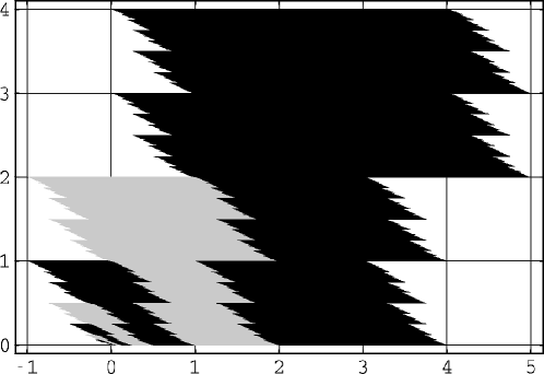
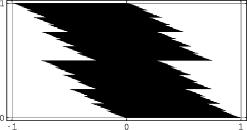
$\mathbf{N}^{2}\left(\mathbf{T}\right)$ showing action of $\mathbf{N}^{-1}$   $\mathbf{T}$ $\mathbf{N}=\left(\begin{smallmatrix}2&1\\ 0&2\end{smallmatrix}\right)$, $D=\left\{\left(\begin{smallmatrix}0\\ 0\end{smallmatrix}\right),\left(\begin{smallmatrix}1\\ 0\end{smallmatrix}\right),\left(\begin{smallmatrix}1\\ 1\end{smallmatrix}\right),\left(\begin{smallmatrix}0\\ 1\end{smallmatrix}\right)\right\}$

Figure 1. Shark-Jawed Parallelogram (Example 9.1)

But

$$\mathbf{N}^{-k}=\frac{1}{4^{k}}\begin{pmatrix}2^{k}&-k2^{k-1}\\ 0&2^{k}\end{pmatrix}$$

so

$$\left\|\mathbf{N}^{-k}\right\|=\frac{1}{4^{k}}\left(2^{k}+k2^{k-1}\right)=\frac{1}{2^{k}}\left(1+\frac{k}{2}\right)\text{.}$$

Hence

$$\left\|R^{n}\begin{pmatrix}x_{1}\\ x_{2}\end{pmatrix}-\mathbf{N}^{-n}\begin{pmatrix}x_{1}\\ x_{2}\end{pmatrix}\right\| \leq\frac{1}{2}\sum_{k=0}^{n-1}\frac{1}{2^{k}}\left(1+\frac{k}{2}\right)$$

$$=\frac{3}{2}+\left(n-3\right)\left(\frac{1}{2}\right)^{n+1}\text{.}$$

But $\lim_{n\rightarrow\infty}\mathbf{N}^{-n}\left(\begin{smallmatrix}x_{1}\\ x_{2}\end{smallmatrix}\right)=0$, and hence

$$\limsup_{n\rightarrow\infty}\left\|R^{n}\begin{pmatrix}x_{1}\\ x_{2}\end{pmatrix}\right\|\leq\frac{3}{2}$$

for any $\left(\begin{smallmatrix}x_{1}\\ x_{2}\end{smallmatrix}\right)\in\mathbb{Z}^{2}$. Thus $R^{n}\left(\begin{smallmatrix}x_{1}\\ x_{2}\end{smallmatrix}\right)$ is contained in the $9$-point set

$$\left\{\begin{pmatrix}y_{1}\\ y_{2}\end{pmatrix}\biggm{|}y_{1},y_{2}=-1,0,1\right\}$$

for $n$ large enough (compare with Lemma 3.8 and Scholium 3.9). Let us compute how $R$ acts on this $9$-point set:

$$\begin{pmatrix}-1\\ -1\end{pmatrix} \overset{\raise 1.0pt\hbox{$\scriptstyle R$}}{\rightarrow}\begin{pmatrix}0\\ -1\end{pmatrix}\overset{\raise 1.0pt\hbox{$\scriptstyle R$}}{\rightarrow}\begin{pmatrix}0\\ -1\end{pmatrix}\rightarrow\cdots$$

$$\begin{pmatrix}-1\\ 0\end{pmatrix} \overset{\raise 1.0pt\hbox{$\scriptstyle R$}}{\rightarrow}\begin{pmatrix}-1\\ 0\end{pmatrix}\overset{\raise 1.0pt\hbox{$\scriptstyle R$}}{\rightarrow}\begin{pmatrix}-1\\ 0\end{pmatrix}\rightarrow\cdots$$

$$\begin{pmatrix}-1\\ 1\end{pmatrix} \overset{\raise 1.0pt\hbox{$\scriptstyle R$}}{\rightarrow}\begin{pmatrix}-1\\ 0\end{pmatrix}\overset{\raise 1.0pt\hbox{$\scriptstyle R$}}{\rightarrow}\begin{pmatrix}-1\\ 0\end{pmatrix}\rightarrow\cdots$$

$$\begin{pmatrix}0\\ -1\end{pmatrix} \overset{\raise 1.0pt\hbox{$\scriptstyle R$}}{\rightarrow}\begin{pmatrix}0\\ -1\end{pmatrix}\rightarrow\cdots$$

$$\begin{pmatrix}0\\ 0\end{pmatrix} \overset{\raise 1.0pt\hbox{$\scriptstyle R$}}{\rightarrow}\begin{pmatrix}0\\ 0\end{pmatrix}\rightarrow\cdots$$

$$\begin{pmatrix}0\\ 1\end{pmatrix} \overset{\raise 1.0pt\hbox{$\scriptstyle R$}}{\rightarrow}\begin{pmatrix}0\\ 0\end{pmatrix}\overset{\raise 1.0pt\hbox{$\scriptstyle R$}}{\rightarrow}\begin{pmatrix}0\\ 0\end{pmatrix}\rightarrow\cdots$$

$$\begin{pmatrix}1\\ -1\end{pmatrix} \overset{\raise 1.0pt\hbox{$\scriptstyle R$}}{\rightarrow}\begin{pmatrix}1\\ -1\end{pmatrix}\rightarrow\cdots$$

$$\begin{pmatrix}1\\ 0\end{pmatrix} \overset{\raise 1.0pt\hbox{$\scriptstyle R$}}{\rightarrow}\begin{pmatrix}0\\ 0\end{pmatrix}\overset{\raise 1.0pt\hbox{$\scriptstyle R$}}{\rightarrow}\begin{pmatrix}0\\ 0\end{pmatrix}\rightarrow\cdots$$

$$\begin{pmatrix}1\\ 1\end{pmatrix} \overset{\raise 1.0pt\hbox{$\scriptstyle R$}}{\rightarrow}\begin{pmatrix}0\\ 0\end{pmatrix}\overset{\raise 1.0pt\hbox{$\scriptstyle R$}}{\rightarrow}\begin{pmatrix}0\\ 0\end{pmatrix}\rightarrow\cdots$$

Thus $R$ has $4$ fixed points,

$$\begin{pmatrix}0\\ 0\end{pmatrix},\begin{pmatrix}0\\ -1\end{pmatrix},\begin{pmatrix}-1\\ 0\end{pmatrix},\begin{pmatrix}1\\ -1\end{pmatrix}\text{,}$$

and $R^{n}\left(\begin{smallmatrix}x_{1}\\ x_{2}\end{smallmatrix}\right)$ is ultimately mapped into one of these fixed points as $n\rightarrow\infty$. Thus the set $B_{\infty}$ defined in Scholium 3.9 just consists of these four fixed points, and there are $4$ atoms in the representation, corresponding to ordinary Cuntz states on $\mathcal{O}_{4}$, by Proposition 5.2 and Corollary 5.3. These states can be computed explicitly using

$$\sigma_{00}\begin{pmatrix}0\\ 0\end{pmatrix} =\begin{pmatrix}0\\ 0\end{pmatrix},$$

$$\sigma_{11}\begin{pmatrix}0\\ -1\end{pmatrix} =\begin{pmatrix}0\\ -1\end{pmatrix},$$

$$\sigma_{10}\begin{pmatrix}-1\\ 0\end{pmatrix} =\begin{pmatrix}-1\\ 0\end{pmatrix},$$

$$\sigma_{01}\begin{pmatrix}1\\ -1\end{pmatrix} =\begin{pmatrix}1\\ -1\end{pmatrix}\text{.}$$

Since these points are fixed by $R$, it follows that the corresponding atoms have period $1$ under the action $\tau$ of $\mathbb{Z}$ on $\left(\mathbb{Z}^{2}\right)^{\approx}$ defined by Theorem 4.1, and hence there are also $4$ cycles, each containing one of the atoms. The four points in $B_{\infty}=\left(-\mathbf{T}\right)\cap\mathbb{Z}^{2}$ for this example are illustrated in Figure 1. (See Proposition 3.12.)

Keeping $\mathbf{N}=\left(\begin{smallmatrix}2&1\\ 0&2\end{smallmatrix}\right)$ the same, but varying $D$, we get a different transformation $R$, see (1.9), and therefore different fixed points: if for example $D^{\prime}=\left\{\left(\begin{smallmatrix}0\\ 0\end{smallmatrix}\right),\left(\begin{smallmatrix}1\\ 0\end{smallmatrix}\right),\left(\begin{smallmatrix}1\\ 1\end{smallmatrix}\right),\left(\begin{smallmatrix}2\\ 1\end{smallmatrix}\right)\right\}$, then we will have the corresponding four periodic points $B^{\prime}_{\infty}=\left\{\left(\begin{smallmatrix}0\\ 0\end{smallmatrix}\right),\left(\begin{smallmatrix}-1\\ 0\end{smallmatrix}\right),\left(\begin{smallmatrix}0\\ -1\end{smallmatrix}\right),\left(\begin{smallmatrix}-1\\ -1\end{smallmatrix}\right)\right\}$. But this second version is an $\mathbf{N}^{2}$-scaled version of the previous one. Note that $\mathbf{N}=\left(\begin{smallmatrix}2&1\\ 0&2\end{smallmatrix}\right)$ yields the transformation

$$\mathbf{N}^{-1}+\mathbf{N}^{-2}+\dots=\left(\mathbf{N}-\hbox{\small 1\kern-3.3pt\normalsize 1}\right)^{-1}=\begin{pmatrix}1&-1\\ 0&1\end{pmatrix}$$

which, for both choices of $D$, maps the points in $D$ onto the vertices in $\mathbf{T}$, and therefore it gets us the integral points in $\mathbf{T}$. This is because all points in $B_{\infty}$ are fixed points in this case; see (3.9).

Scholium 3.9 is a universal algorithm allowing an explicit calculation of all of the $R$-periodic points $B_{\infty}=\left(-\mathbf{T}\right)\cap\mathbb{Z}^{\nu}$ for general pairs $\mathbf{N},D$ (as described) in $\nu$ dimensions, and (5.9)–(5.12) in Remark 5.5 is in principle an abstract and general formula yielding all the integral points in $\mathbf{T}$ in any dimension $\nu$. But the only general way to solve (5.9) seems to be to use Scholium 3.9. In the examples of the Figures, $k$ from (5.9) is $1$. In Example 9.8, we also need $k=2$.

For other related matrix applications of this type, we refer to [Ban96], [Pri], [BreJo], [Han], and [PoPr].

9.2. Another matrix case: full spectrum

An instance where the estimate (3.17) is in fact an equality in an equivalent norm is when the matrix $\mathbf{N}$ satisfies $\mathbf{N}^{m}=p\hbox{\small 1\kern-3.3pt\normalsize 1}_{\nu}$ for some integer values $m$, $p$, i.e., $m\in\left\{2,3,\dots\right\}$, $p\in\mathbb{Z}$. This is a special case of the situation in Remark 5.5, but with the added simplification that $\mathbf{N}^{m}$ is now a scalar.

Remark 9.2.

Semisimple matrices $\mathbf{N}$. Suppose there are integers $m$, $p$ as described such that $\mathbf{N}^{m}=p\hbox{\small 1\kern-3.3pt\normalsize 1}_{\nu}$.

1. Then the matrix $\mathbf{N}$ is diagonalizable with spectrum $\left\{\lambda_{k}\right\}$ of the form $\lambda_{k}=N^{\frac{1}{\nu}}e^{i\theta_{k}}=\left|p\right|^{\frac{1}{m}}e^{i\theta_{k}}$, where $N=\left|\det\mathbf{N}\right|$, and necessarily $m\theta_{k}\in 2\pi\mathbb{Z}$.

2. Let $D\subset\mathbb{Z}^{\nu}$ be a full set of residues for $\mathbf{N}$ as described. If, for some $d\in D$, the solution in $\mathbb{R}^{\nu}$ to $d+\mathbf{N}x=x$ is integral (i.e., $x\in\mathbb{Z}^{\nu}$) (and then $x=R\left(x\right)$), then the point

   $$d^{\prime}:=d+\mathbf{N}d+\dots+\mathbf{N}^{m-1}d\in D^{\prime}:=D+\mathbf{N}D+\dots+\mathbf{N}^{m-1}D$$

   satisfies $d^{\prime}+px=x$; in particular, $x\in\left(1-p\right)^{-1}D^{\prime}$.

3. If there are points $d_{1},\dots,d_{k}\in D$ such that the solution $x$ to

   $$d_{1}+\mathbf{N}d_{2}+\dots+\mathbf{N}^{k-1}d_{k}+\mathbf{N}^{k}x=x$$

   is integral, i.e., $x\in\mathbb{Z}^{\nu}$ (and then $x=R^{k}\left(x\right)$) then there are also points $d_{1}^{\prime},\dots,d_{k}^{\prime}\in D^{\prime}$ such that

   $$d_{1}^{\prime}+pd_{2}^{\prime}+\dots+p^{k-1}d_{k}^{\prime}+p^{k}x=x\text{.}$$

Proof.

Points $\lambda_{k}\in\mathop{\rm spec}\left(\mathbf{N}\right)$ must satisfy $\lambda_{k}^{m}=p$, so the root-of-unity assertion in (i) follows. The matrix $\mathbf{N}$ is diagonalizable because its minimal polynomial must divide $x^{m}-p$. Note that the eigenvalues of $\mathbf{N}$ need not have uniform multiplicity over $\mathbb{Z}_{m}$ by Example 9.7 below.

It follows that, if $m\in\mathbb{N}$ is chosen minimal $\mathrm{s.t.}$ $\mathbf{N}^{m}=p\hbox{\small 1\kern-3.3pt\normalsize 1}_{\nu}$ for some $p\in\mathbb{Z}$, then the minimal polynomial of $\mathbf{N}$ equals $x^{m}-p$ iff $\mathop{\rm spec}\left(\mathbf{N}\right)=\left\{N^{\frac{1}{\nu}}e^{i2\pi\frac{k}{m}}\right\}_{k=0}^{m-1}$, with the minimal polynomial defined as the monic minimal degree polynomial $\phi\left(x\right)\in\mathbb{C}\left[x\right]$ satisfying $\phi\left(\mathbf{N}\right)=0$. Note that, in general, we have $\phi\left(x\right)$ dividing $x^{m}-p$; and $\phi\left(x\right)$ dividing $\det\left(x\hbox{\small 1\kern-3.3pt\normalsize 1}_{\nu}-\mathbf{N}\right)$. If $p\neq 0$ is square-free and $p\neq\pm 1$, then $x^{m}-p$ is irreducible over $\mathbb{Q}$, by Eisenstein; and so $\phi\left(x\right)=x^{m}-p$ also divides $\det\left(x\hbox{\small 1\kern-3.3pt\normalsize 1}_{\nu}-\mathbf{N}\right)$.

For Examples 9.7–9.8 below, $\mathbf{N}=\left(\begin{smallmatrix}1&-1\\ 1&1\end{smallmatrix}\right)$, resp., $\mathbf{N}=\left(\begin{smallmatrix}0&1\\ 4&0\end{smallmatrix}\right)$, we have the minimality condition satisfied for $m=4$, $p=-4$; resp., $m=2$, $p=4$. In the second example, all three polynomials $\phi\left(x\right)$, $x^{m}-p$, and $\det\left(x\hbox{\small 1\kern-3.3pt\normalsize 1}_{\nu}-\mathbf{N}\right)$ coincide; whereas in the first example $x^{m}-p=x^{4}+4$ while $\phi\left(x\right)=\det\left(x\hbox{\small 1\kern-3.3pt\normalsize 1}_{\nu}-\mathbf{N}\right)=x^{2}-2x+2$, and $\mathop{\rm spec}\left(\mathbf{N}\right)=\left\{\sqrt{2}e^{\pm i\frac{\pi}{4}}\right\}$.

(ii): Given the points $d$, $x$ as specified in (ii), i.e., $d+\mathbf{N}x=x$, we have

$$\left(1-p\right)x =\left(\hbox{\small 1\kern-3.3pt\normalsize 1}-\mathbf{N}^{m}\right)x$$

$$=\left(\hbox{\small 1\kern-3.3pt\normalsize 1}+\mathbf{N}+\dots+\mathbf{N}^{m-1}\right)\left(\hbox{\small 1\kern-3.3pt\normalsize 1}-\mathbf{N}\right)x$$

$$=\left(\hbox{\small 1\kern-3.3pt\normalsize 1}+\mathbf{N}+\dots+\mathbf{N}^{m-1}\right)d$$

$$=d+\mathbf{N}d+\dots+\mathbf{N}^{m-1}d=d^{\prime}\text{,}$$

which is the assertion.

(iii): Setting $e:=d_{1}+\mathbf{N}d_{2}+\dots+\mathbf{N}^{k-1}d_{k}$, and iterating the given equation, we get

$$x =e+\mathbf{N}^{k}x=e+\mathbf{N}^{k}e+\mathbf{N}^{2k}x=\dots$$

$$=e+\mathbf{N}^{k}e+\mathbf{N}^{2k}e+\dots+\mathbf{N}^{k\left(m-1\right)}e+\mathbf{N}^{km}x$$

$$=\left(\hbox{\small 1\kern-3.3pt\normalsize 1}+\mathbf{N}^{k}+\dots+\mathbf{N}^{k\left(m-1\right)}\right)e+p^{k}x\text{.}$$

The individual terms in the sum are

$$\sum_{i<m}\mathbf{N}^{ik}e=\sum_{i<m}\sum_{j<k}\mathbf{N}^{ik+j}d_{j}=\sum_{j<k}\sum_{i<m}\mathbf{N}^{ik+j}d_{j}=\sum_{l<k}\sum_{r<m}\mathbf{N}^{lm+r}d_{l\left(r\right)}=\sum_{l<k}p^{l}d_{l}^{\prime}\text{,}$$

where $d_{l}^{\prime}=\sum_{r<m}\mathbf{N}^{r}d_{l\left(r\right)}$.∎

The equation $\mathbf{N}^{m}=p\hbox{\small 1\kern-3.3pt\normalsize 1}_{\nu}$ arises in the study of tilings as they are used in wavelet theory; see, e.g., [DDL], [Ban91], [Hou], [HRW], and [LaWa2]. Candidates for dual objects for our discrete orbits in $\mathbb{Z}^{\nu}$, and corresponding to the given data $\left(\mathbf{N},D\right)$, are the sets introduced in (3.11) and (3.12):

$$\mathbf{T}=T\left(\mathbf{N},D\right):=\left\{\sum_{i=1}^{\infty}\mathbf{N}^{-i}d_{i}\biggm{|}d_{i}\in D\right\}\text{.}$$

Recall that if the $\nu$-dimensional Lebesgue measure of $\mathbf{T}$ is one, i.e., $\mu_{\nu}\left(T\left(\mathbf{N},D\right)\right)=1$, then $\mathbf{T}$ is a periodic tile, i.e.,

$$\bigcup_{n\in\mathbb{Z}^{\nu}}\left(\mathbf{T}+n\right)=\mathbb{R}^{\nu}$$

and $\mu_{\nu}\left(\mathbf{T\cap}\left(\mathbf{T}+n\right)\right)=0$ for $n\in\mathbb{Z}^{\nu}$, $n\neq 0$. The $\mu_{\nu}$-measure-one condition is true in our case since there are $m$, $p$ such that $\mathbf{N}^{m}=p\hbox{\small 1\kern-3.3pt\normalsize 1}$. Recall also from Proposition 3.12 that we may recover $B_{\infty}$ as $B_{\infty}=\mathbb{Z}^{\nu}\cap\left\{-\mathbf{T}\right\}$. For Example 9.1, above, the tile $\mathbf{T}$ is the parallelogram in Figure 1, above, and we see from this figure that $B_{\infty}=-\left\{\left(\begin{smallmatrix}0\\ 0\end{smallmatrix}\right),\left(\begin{smallmatrix}0\\ 1\end{smallmatrix}\right),\left(\begin{smallmatrix}1\\ 0\end{smallmatrix}\right),\left(\begin{smallmatrix}-1\\ 1\end{smallmatrix}\right)\right\}$ in accordance with Proposition 3.12. The appearance of this tile can be explained as follows: from (3.12) and the expression for $\mathbf{N}^{-k}$ in Example 9.1, it follows that

$$\sum_{k=1}^{\infty}\mathbf{N}^{-k}d_{k}=\begin{pmatrix}x-\phi\left(y\right)\\ y\end{pmatrix}$$

if $d_{k}=\begin{pmatrix}i_{k}\\ j_{k}\end{pmatrix}$, $i_{k},j_{k}=0,1$, where

$$x=\sum_{k}\frac{1}{2^{k}}i_{k}\text{,\quad}y=\sum_{k}\frac{1}{2^{k}}j_{k}$$

are arbitrary numbers in the interval $\left[0,1\right]$, given in dyadic expansion. The function $\phi$, defined by

$$\phi\left(y\right)=\sum_{k}\frac{k}{2^{k+1}}j_{k}\text{,}$$

is strictly speaking not a function of $y\in\left[0,1\right]$ alone, but depends on the particular dyadic expansion used for $y$ (that is, $\phi$ is a function on the Cantor set obtained by cutting and doubling points at each dyadic rational in $\left[0,1\right]$). Now, if $y$ is the dyadic rational $y=p2^{-k}$, where $1\leq p\leq 2^{k}-1$ and $p$ is odd, then $j_{k}=1$, and

$$y=\frac{p-1}{2}2^{-k+1}+2^{-k}=\frac{p-1}{2}2^{-k+1}+\sum_{l=k+1}^{\infty}2^{-l}\text{.}$$

Thus

$$\phi\left(y_{+}\right)=\phi\left(y\right)=\phi\left(\frac{p-1}{2}2^{-k+1}\right)+k2^{-k-1}$$

and

$$\phi\left(y_{-}\right)=\phi\left(\frac{p-1}{2}2^{-k+1}\right)+\sum_{l=k+1}^{\infty}l2^{-l-1}\text{.}$$

Thus $\phi$ is continuous everywhere except at the dyadic rationals, and $\phi$ is continuous to the right even at the dyadic rationals. If $y=p2^{-k}$ with $p$ odd, we have

$$\phi\left(y_{+}\right)-\phi\left(y_{-}\right)=k2^{-k-1}-\sum_{l=k+1}^{\infty}l2^{-l-1}=-2^{-k}\text{.}$$

Now, since

$$\mathbf{T}=\left\{\begin{pmatrix}x-\phi\left(y\right)\\ y\end{pmatrix}\biggm{|}\begin{pmatrix}x\\ y\end{pmatrix}\in\left[0,1\right]\times\left[0,1\right]\right\}=\bigcup_{y\in\left[0,1\right]}\begin{pmatrix}\left[-\phi\left(y\right),-\phi\left(y\right)+1\right]\\ y\end{pmatrix}$$

this explains the appearance of the shark-jawed parallelogram in Figure 1 above. In particular, the teeth constitute the graph of the function $\phi$, and one sees that at $y=\frac{1}{2}$ the graph makes a jump of $-\frac{1}{2}$, and at $y=\frac{1}{4}$ and $\frac{3}{4}$ the graph makes a jump of $-\frac{1}{4}$, etc., in accordance with the description above of $\phi$.

9.3. Self-similarity and tiles

The more detailed tiling properties of $\mathbf{T}$ give us a precise way of relating properties of the mapping $R$ from (1.9) to our Fourier representation (1.8) for the $\mathcal{O}_{N}$-representation, and then back to the $\ell^{2}$-basis viewpoint in Section 4. If $\mathbf{T}$ is in fact a $\mathbb{Z}^{\nu}$-tile for $\mathbb{R}^{\nu}$, then it follows from [Jor95] that the $L^{2}\left(\mathbb{T}^{\nu}\right)$ representation in (1.8) is unitarily equivalent to a representation on $L^{2}\left(\mathbf{T}\right)$, where the measure on $\mathbf{T}$ is simply the restriction of the $\mathbb{R}^{\nu}$-Lebesgue measure. The mapping $z\mapsto z^{\mathbf{N}}$ of $\mathbb{T}^{\nu}$ into itself in (1.8) is then equivalent to the endomorphism $\tau$ on $\mathbf{T}$ defined as follows: let $t\in\mathbf{T}$; pick the unique representation: $\mathbf{N}t=s+n$, $s\in\mathbf{T}$, $n\in\mathbb{Z}^{\nu}$, and then define $\tau\left(t\right)=s$. This gives a concrete realization of our symbolic coding mappings $\sigma_{i}$ and $R$ from (6.1) and (6.2), respectively. For, if $D$ is represented as $D=\left\{d_{i}\right\}_{i=1}^{N}$, and $\tau_{i}\left(x\right):=\mathbf{N}^{-1}\left(x+d_{i}\right)$, then $\tau_{i}:\mathbf{T}\rightarrow\mathbf{T}$, and $\tau\circ\tau_{i}=\mathop{\rm id}_{\mathbf{T}}$ for all $i=1,\dots,N$. So $\tau$ is a fractal version of the integral mapping $R$ in (6.2).

More generally, suppose $0\in D$, and $D$ is a full set of residues, i.e., a selection of a point in $\mathbb{Z}^{\nu}$ for each of the $N$ cosets of $\mathbb{Z}^{\nu}\diagup\mathbf{N}\mathbb{Z}^{\nu}$. Then let $\mathbb{L\kern 0.5pt}:=\mathbb{Z}\left(\mathbf{N},D\right)$ be the smallest $\mathbf{N}$-invariant lattice containing $D$, and suppose $\mathbf{T}$ tiles by $\mathbb{L\kern 0.5pt}$. Then, using that $\mathbf{N}\mathbb{L\kern 0.5pt}\subset\mathbb{L\kern 0.5pt}$, note that $\tau:\mathbf{T}\rightarrow\mathbf{T}$ may be defined as before: $\mathbf{N}t=s+n$, $t,s\in\mathbf{T}$, $n\in\mathbb{L\kern 0.5pt}$, $\tau\left(t\right)=s$; and we will still have the formula $\tau\circ\tau_{i}=\mathop{\rm id}_{\mathbf{T}}$ from above, but now in the more general case. In fact (3.11) shows that $\tau_{i}$ and $\tau$ may be defined on $\mathbf{T}$ independently of $\mathbb{L\kern 0.5pt}$. (See also the discussion in Scholium 9.5 below, especially the conclusion (9.7) there. We may then define a representation of $\mathcal{O}_{N}$ on $L^{2}\left(\mathbf{T}\right)$ by the following explicit formulas for the operators:

(9.1) $$S_{i}\psi =N^{\frac{1}{2}}\chi_{\tau_{i}\left(\mathbf{T}\right)}\psi\circ\tau$$

and

(9.2) $$S^{*}_{i}\psi =N^{-\frac{1}{2}}\psi\circ\tau_{i}\quad\left(\psi\in L^{2}\left(\mathbf{T}\right)\right)\text{.}$$

The argument for why the $\mathcal{O}_{N}$-relations (2.3) are indeed satisfied for the operators $S_{i}$ defined in (9.1) is from [JoPe94]. Indeed the orthogonality relation in (2.3) is clear, and $\sum_{i}S_{i}S^{*}_{i}=\hbox{\small 1\kern-3.3pt\normalsize 1}$ follows from (3.11) combined with the formula (9.2) for $S^{*}_{i}$. We also use the basic properties of the Lebesgue measure, when restricted to $\mathbf{T}$: we have, for $\psi\in L^{2}\left(\mathbf{T}\right)$,

$$\sum_{i}\left\langle\psi\mid S_{i}S^{*}_{i}\psi\right\rangle =\sum_{i}\left\|S^{*}_{i}\psi\right\|^{2}=\sum_{i}N^{-1}\int_{\mathbf{T}}\left|\psi\circ\tau_{i}\right|^{2}\,dx$$

$$=\sum_{i}N^{-1}\int_{\mathbf{T}}\left|\psi\left(\mathbf{N}^{-1}\left(x+d_{i}\right)\right)\right|^{2}\,dx$$

$$=\int_{\mathbf{T}}\left|\psi\right|^{2}\,dx=\left\langle\psi\mid\psi\right\rangle\text{,}$$

where (3.11), and the corresponding formula for Lebesgue measure, was used in the last step. If $\mathbf{T}$ is not a $\mathbb{Z}^{\nu}$-tile, it is still a finite covering of the torus $\mathbb{T}^{\nu}$, as long as $D$ is assumed to be a full set of residues for $\mathbb{Z}^{\nu}\diagup\mathbf{N}\mathbb{Z}^{\nu}$, as follows from [JoPe92, Theorem 6.2], which also gives an expression for the covering number. We refer to [JoPe92, Theorem 6.2] for the definition of a finite covering: what is implied here is that $\mathbf{T}=\bigcup_{i=1}^{q}E_{i}$ where the $E_{i}$’s are $\mathbb{Z}^{\nu}$-periodic tiles, and where the intersections $E_{i}\cap E_{j}$, $i\neq j$, have $\nu$-dimensional Lebesgue measure equal to zero. In particular, we conclude that the Lebesgue measure of $\mathbf{T}$ must be an integer. To apply Theorem 6.2 in [JoPe92] we first show that $\left\{e_{n}\left(x\right):=e^{i2\pi n\cdot x}\right\}$, $x\in\mathbf{T}$, $n\in\mathbb{Z}^{\nu}$, is an orthogonal family in $L^{2}\left(\mathbf{T}\right)$, relative to the restricted Lebesgue measure. In general, $\left\{e_{n}|_{\mathbf{T}}\right\}_{n\in\mathbb{Z}^{\nu}}$ will not be a basis for $L^{2}\left(\mathbf{T}\right)$. For that it is necessary and sufficient that $\mathbf{T}$ be a $\mathbb{Z}^{\nu}$-tile. But the functions are always mutually orthogonal in $L^{2}\left(\mathbf{T}\right)$. For the general theory, see [LiMa].

We now turn to the specifics of the aforementioned application of [JoPe92, Theorem 6.2]. It is based on the following general fact.

Proposition 9.3.

Let $\mathbf{N},D,\mathbf{T}$ be as described above (i.e., with the eigenvalues $\lambda_{i}$ of $\mathbf{N}$ satisfying $\left|\lambda_{i}\right|>1$, $D$ a full set of residues for $\mathbb{Z}^{\nu}\diagup\mathbf{N}\mathbb{Z}^{\nu}$, and $\mathbf{T}$ the fractal determined by (3.11)). We then have

$$\int_{\mathbf{T}}e_{n}\left(x\right)\,dx=0$$

for all $n\in\mathbb{Z}^{\nu}\,\diagdown\left\{0\right\}$; and therefore $\mathbf{T}$ is a finite cover space for the torus $\mathbb{T}^{\nu}=\mathbb{R}^{\nu}\diagup\mathbb{Z}^{\nu}$.

Proof.

Let $\mathbf{N},D$ be given as specified, and let $\mathbf{M}$ denote the transposed matrix $\mathbf{N}^{\mathop{\rm tr}}$. For $x\in\mathbb{R}^{\nu}$, let

$$F_{D}\left(x\right):=\sum_{d\in D}e^{i2\pi x\cdot d}=\sum_{d\in D}e_{d}\left(x\right)\text{.}$$

An iteration of (3.11) in the form $\mathbf{T}=\bigcup_{d\in D}\mathbf{N}^{-1}\left(d+\mathbf{T}\right)$ then yields the following product formula:

$$\int_{\mathbf{T}}e_{n}\left(x\right)\,dx=F\left(\mathbf{M}^{-1}n\right)F\left(\mathbf{M}^{-2}n\right)\cdots F\left(\mathbf{M}^{-k}n\right)\int_{\mathbf{N}^{-k}\mathbf{T}}e_{n}\left(x\right)\,dx\text{,}$$

valid for all $n\in\mathbb{Z}^{\nu}$, $k=1,2,\dots$, and where $dx$ denotes the $\nu$-dimensional Lebesgue measure. Assuming $n\in\mathbb{Z}^{\nu}\,\diagdown\left\{0\right\}$, use (3.7) for the matrix $\mathbf{M}$, and pick $k$ large enough to get a non-trivial residue for $n$, taking into account (3.8). We will then have

$$F\left(\mathbf{M}^{-1}n\right)=\cdots=F\left(\vphantom{\mathbf{M}^{-1}}\smash{\mathbf{M}^{-\left(k-1\right)}n}\right)=N\text{,}$$

and $F\left(\mathbf{M}^{-k}n\right)=0$; and the result from the Proposition follows. Indeed, if $n\in\mathbb{Z}^{\nu}\,\diagdown\left\{0\right\}$, then there is some $k\in\mathbb{N}$, and $n^{\prime},r\in\mathbb{Z}^{\nu}$, such that $n=\mathbf{M}^{k}n^{\prime}+\mathbf{M}^{k-1}r$ and $r\notin\mathbf{M}\left(\mathbb{Z}^{\nu}\right)$. We then get

$$F_{D}\left(\mathbf{M}^{-k}n\right)=F_{D}\left(n^{\prime}+\mathbf{M}^{-1}r\right)=\sum_{d\in D}e_{d}\left(n^{\prime}+\mathbf{M}^{-1}r\right)=\sum_{d\in D}e_{d}\left(\mathbf{M}^{-1}r\right)\text{.}$$

But now we can use $D$ as a set of representatives for the elements in the finite group $\mathbb{Z}^{\nu}\diagup\mathbf{N}\left(\mathbb{Z}^{\nu}\right)$. Since $\mathbf{M}^{-1}r\notin\mathbb{Z}^{\nu}$, the last sum is an average of a non-trivial character on a finite group, and so it is zero by a standard fact about group characters. Indeed, replacing $D=\left\{d_{i}\right\}_{i=1}^{N}$ with $d_{i}^{\prime}=d_{i}+\mathbf{N}l_{i}$, for any $l_{i}\in\mathbb{Z}^{\nu}$, will not affect the sum. It then follows from [JoPe92, Theorem 6.2] that $\mathbf{T}$ is a finite cover of the standard torus. ∎

As a consequence, in the general case, even when $\mathbf{T}$ is not a $\mathbb{Z}^{\nu}$-tile, our $\mathcal{O}_{N}$-representations are realized on $L^{2}\left(\mathbf{T}\right)$ in the same manner as in the special case (9.1)–(9.2). The representation on $L^{2}\left(\mathbf{T}\right)$ which is defined by (9.1) is not unitarily equivalent to our original permutative representation on $\ell^{2}\left(\mathbb{Z}^{\nu}\right)$ from (1.8) (or, equivalently, from (3.7)). But when (9.1) is adjusted by a cocycle as described in [BJP, Section 2], then the old representation on $\ell^{2}\left(\mathbb{Z}^{\nu}\right)\simeq L^{2}\left(\mathbb{T}^{\nu}\right)$ will be contained in the corresponding (adjusted) representation on $L^{2}\left(\mathbf{T}\right)$ where the intertwining operator $W:\ell^{2}\left(\mathbb{Z}^{\nu}\right)\rightarrow L^{2}\left(\mathbf{T}\right)$ is the one which takes the basis $\left\{e_{n}:n\in\mathbb{Z}^{\nu}\right\}$ for $\ell^{2}\left(\mathbb{Z}^{\nu}\right)$ into the functions $f_{n}\left(x\right)=e^{i2\pi n\cdot x}$, restricted to $\mathbf{T}$, i.e., $x\in\mathbf{T}:We_{n}=f_{n}$, $n\in\mathbb{Z}^{\nu}$. As an application of Proposition 9.3, we note that the two representations, the “old” one (3.7), and the new one on $L^{2}\left(\mathbf{T}\right)$, will be unitarily equivalent iff $\mathbf{T}$ is a $\mathbb{Z}^{\nu}$-tile. The present section has examples of both $\mathbf{T}$ having this $\mathbb{Z}^{\nu}$-tiling property, and not: Example $D_{1}$ has it (see Figure 4), while $D_{3}$, $D_{5}$, and $D_{9}$ do not (see Figures 5, 7, and 8).

Theorem 9.4.

Let $\left(\mathbf{N},D\right)$ be as in Proposition 9.3. Let $\mathbf{M}:=\mathbf{N}^{\mathop{\rm tr}}$ be the transposed matrix, and let $G=\left\{r_{j}\right\}_{j=1}^{N}\subset\mathbb{Z}^{\nu}$ be a full set of residues for $\mathbf{M}$ such that $N^{-\frac{1}{2}}\left(e^{i2\pi r_{j}\cdot\mathbf{N}^{-1}d_{k}}\right)_{jk}$ is unitary as an $N\times N$ matrix. Given $D$, a corresponding $G$ can be found by group duality. Let $\left\{V_{j}\right\}$ be the representation of $\mathcal{O}_{N}$ which is determined by $\left(\mathbf{M},G\right)$ and (3.7), i.e., $V_{j}e_{n}=e_{r_{j}+\mathbf{M}n}$, $n\in\mathbb{Z}^{\nu}$, and let $W:\ell^{2}\left(\mathbb{Z}^{\nu}\right)\rightarrow L^{2}\left(\mathbf{T}\right)$ be the isometry which is given by $e_{n}\mapsto f_{n}$ according to Proposition 9.3. Let $m_{ji}:=N^{-\frac{1}{2}}f_{r_{i}}\circ\tau_{j}$, and $T_{i}:=\sum_{j=1}^{N}S_{j}m_{ji}$, where $\left\{S_{j}\right\}$ is given by (9.1). Then $W$ intertwines, i.e.,

(9.3) $$WV_{i}=T_{i}W\text{,\quad}i=1,\dots,N\text{.}$$

Proof.

See the formulas in Section 3 for the $\mathbf{N}$ representations, and Section 2 in [BJP]. The modified formulas (9.1)–(9.2) for the $L^{2}\left(\mathbf{T}\right)$-representations may be written in the following explicit form: let $\left(\mathbf{N},D\right)$ and $\left(\mathbf{M},G\right)$ be chosen as before in duality, i.e., $D=\left\{d_{i}\right\}_{i=1}^{N}$ and $G=\left\{r_{i}\right\}_{i=1}^{N}$ residue sets in $\mathbb{Z}^{\nu}$ as described. The duality condition will be satisfied for the pair if, e.g.,

(9.4) $$r_{j}\cdot\mathbf{N}^{-1}\left(d_{k}\right)\in\frac{\left(j-1\right)\left(k-1\right)}{N}+\mathbb{Z}$$

for all $j,k\in\left\{1,2,\dots,N\right\}$, where $N=\left|\det\mathbf{N}\right|$ as usual. This choice will work if $N$ is a prime. Then we claim that the representation $\left\{T_{i}\right\}$ on $L^{2}\left(\mathbf{T}\right)$ contains a copy of the original $\mathcal{O}_{N}$-representation on $\ell^{2}\left(\mathbb{Z}^{\nu}\right)$. It is determined by:

($$\ref{Up}^{\prime} T_{i}\psi =f_{r_{i}}\left.\psi\circ\tau\right.\text{,}$$)

and

($$\ref{Down}^{\prime} T^{*}_{i}\psi =\frac{1}{N}\sum_{j=1}^{N}\overline{f_{r_{i}}\circ\tau_{j}}\left.\psi\circ\tau_{j}\right.\quad\left(\psi\in L^{2}\left(\mathbf{T}\right)\right)\text{,}$$)

where $\tau$ and $\tau_{j}$ are the mappings on $\mathbf{T}$ from $\left(\mathbf{N},D\right)$ as in (9.1)–(9.2). Notice that ($\ref{Up}^{\prime}$) should be compared to (1.8) from the Introduction, and the unitarity condition for the $N\times N$ matrix in Theorem 9.4 is a generalization of the condition on the matrix (1.1).The basic idea behind the isometric intertwiner

(9.5) $$We_{n}=f_{n}=e^{i2\pi n\cdot x}\text{,\quad}n\in\mathbb{Z}^{\nu},\;x\in\mathbf{T}\text{,}$$

is from [JoPe92] and [JoPe94] (which also contain more details on this point).

Firstly, it is immediate from ($\ref{Up}^{\prime}$) that the intertwining relation (9.3) holds on $\ell^{2}\left(\mathbb{Z}^{\nu}\right)$, where the $\mathcal{O}_{N}$-representation $\left\{V_{i}\right\}$, acting on $\ell^{2}\left(\mathbb{Z}^{\nu}\right)$, is given by the formula

(9.6) $$V_{i}e_{n}=e_{r_{i}+\mathbf{M}n}\text{,\quad}n\in\mathbb{Z}^{\nu}$$

on the canonical basis vectors. Indeed, for $n\in\mathbb{Z}^{\nu}$, $x\in\mathbf{T}$,

$$T_{i}We_{n}\left(x\right)=f_{r_{i}}\left(x\right)f_{n}\left(\mathbf{N}x\right)=f_{r_{i}}\left(x\right)f_{\mathbf{M}n}\left(x\right)=f_{r_{i}+\mathbf{M}n}\left(x\right)=WV_{i}e_{n}\left(x\right)\text{,}$$

proving (9.3).

We now show that $\left\{T_{i}\right\}$ satisfies the $\mathcal{O}_{N}$-relations (2.3), and that, in addition to (9.3), we also have

$$T^{*}_{i}W=WV^{*}_{i}\text{,\quad}i=1,\dots,N\text{.}$$

To see that $\sum_{i}T_{i}T^{*}_{i}=\hbox{\small 1\kern-3.3pt\normalsize 1}$ on $L^{2}\left(\mathbf{T}\right)$, we proceed as follows: let $\psi\in L^{2}\left(\mathbf{T}\right)$. Then

$$\sum_{i}\left\|T^{*}_{i}\psi\right\|^{2} =\sum_{i}\frac{1}{N^{2}}\int_{\mathbf{T}}\left|\smash{\sum_{j}\overline{f_{r_{i}}\circ\tau_{j}}\left.\psi\circ\tau_{j}\right.}\vphantom{\sum f}\right|^{2}\,dx$$

$$=\frac{1}{N^{2}}\sum_{j}\sum_{k}\int_{\mathbf{T}}\sum_{i}\overline{f_{r_{i}}\circ\tau_{j}}\left.f_{r_{i}}\circ\tau_{k}\right.\left.\psi\circ\tau_{j}\right.\overline{\psi\circ\tau_{k}}\,dx$$

$$=\frac{1}{N}\sum_{j}\sum_{k}\delta_{jk}\int_{\mathbf{T}}\left|\psi\right|^{2}\circ\tau_{j}\,dx=\frac{1}{N}\sum_{j}\int_{\mathbf{T}}\left|\psi\right|^{2}\circ\tau_{j}\,dx$$

$$=\int_{\mathbf{T}}\left|\psi\right|^{2}\,dx$$

which is the desired conclusion.

We claim that $\ell^{2}\left(\mathbb{Z}^{\nu}\right)$ in fact defines a subrepresentation of $\mathcal{O}_{N}$ in $L^{2}\left(\mathbf{T}\right)$ in the strict sense: indeed, let $\ell^{2}\left(\mathbb{Z}^{\nu}\right)$ be viewed as a subspace of $L^{2}\left(\mathbf{T}\right)$ via the isometry $W$, and let $V_{i}$ define the original $\ell^{2}\left(\mathbb{Z}^{\nu}\right)$ representation by (9.6). There are then operators $U_{i}$, $B_{i}$, defined on $L^{2}\left(\mathbf{T}\right)\ominus\ell^{2}\left(\mathbb{Z}^{\nu}\right)$, such that

$$T_{i}=\begin{pmatrix}V_{i}&B_{i}\\ 0&U_{i}\end{pmatrix}\text{,\quad}i=1,\dots,N\text{.}$$

The exact form of the complementary operators $B_{i}$, $U_{i}$ can be read off from ($\ref{Up}^{\prime}$)–($\ref{Down}^{\prime}$), and they are both zero precisely when $\mathbf{T}$ is a $\mathbb{Z}^{\nu}$-tile. Since both systems $\left\{V_{i}\right\}$ and $\left\{T_{i}\right\}$ satisfy the Cuntz relations (2.3) in the respective Hilbert spaces, we get

$$\sum_{i}\left(V_{i}V^{*}_{i}+B_{i}B^{*}_{i}\right)=\hbox{\small 1\kern-3.3pt\normalsize 1}\text{,}$$

and therefore $B_{i}=0$ for all $i$. It follows that $T_{i}=\left(\begin{smallmatrix}V_{i}&0\\ 0&U_{i}\end{smallmatrix}\right)$, and that the operators $U_{i}$ also define an $\mathcal{O}_{N}$-representation, now on $L^{2}\left(\mathbf{T}\right)\ominus\ell^{2}\left(\mathbb{Z}^{\nu}\right)$. ∎

Scholium 9.5.

In summary, we have shown that, for every pair $\left(\mathbf{M},G\right)$ in $\mathbb{Z}^{\nu}$ (i.e., $G$ a full set of residues for $\mathbb{Z}^{\nu}\diagup\mathbf{M}\mathbb{Z}^{\nu}$), there is a dual pair $\left(\mathbf{N},D\right)$ (see (9.4)) such that the $\mathcal{O}_{N}$-representation defined from $\left(\mathbf{M},G\right)$ on $\ell^{2}\left(\mathbb{Z}^{\nu}\right)$ by (9.6) is unitarily equivalent to a subrepresentation of the $\mathcal{O}_{N}$-representation on $L^{2}\left(\mathbf{T}\right)$ defined from $\left(\mathbf{N},D\right)$ via formulas ($\ref{Up}^{\prime}$)–($\ref{Down}^{\prime}$). The intertwining isometry $\ell^{2}\left(\mathbb{Z}^{\nu}\right)\overset{\smash[b]{\lower 1.0pt\hbox{$\scriptstyle W$}}}{\hookrightarrow}L^{2}\left(\mathbf{T}\right)$ is the one defined from Proposition 9.3; see (9.5).

We also note that the orthogonality condition in Proposition 9.3 generally holds for a larger lattice than $\mathbb{Z}^{\nu}$. In fact, given $\left(\mathbf{N},D\right)$, $0\in D$, as before, we introduced the smallest lattice $\mathbb{L\kern 0.5pt}$ containing $D$ and invariant under $\mathbf{N}$, and the corresponding dual lattice

$$\mathbb{L\kern 0.5pt}^{*}=\left\{\xi\in\mathbb{R}^{\nu}\mid\xi\cdot\lambda\in\mathbb{Z},\forall\lambda\in\mathbb{L\kern 0.5pt}\right\}\text{.}$$

Using the same argument as from the proof of Proposition 9.3 and (9.4), we can show that, in fact,

(9.7) $$\int_{\mathbf{T}}f_{\xi}\left(x\right)\,dx=0\text{,\quad}\forall\xi\in\mathbb{L\kern 0.5pt}^{*}\,\diagdown\left\{0\right\}\text{.}$$

For those special cases when $\mathbf{T}$ is already an $\mathbb{L\kern 0.5pt}$-periodic tile (for example, for some of the “cloud” examples in Examples 9.11 and 9.14 below, e.g. $D_{3}$ and $D_{5}$ in (9.13)), we then conclude from formulas ($\ref{Up}^{\prime}$), (9.3), and (9.6) above that the $\left\{T_{i}\right\}$-representation of $\mathcal{O}_{N}$ on $L^{2}\left(\mathbf{T}\right)$ is then permutative. The argument is also based on the following simple implication: $\mathbf{N}\left(\mathbb{L\kern 0.5pt}\right)\subset\mathbb{L\kern 0.5pt}\Rightarrow\mathbf{M}\left(\mathbb{L\kern 0.5pt}^{*}\right)\subset\mathbb{L\kern 0.5pt}^{*}$, when $\mathbf{M}=\mathbf{N}^{\mathop{\rm tr}}$. Also recall $\left(\mathbf{N}\mathbb{Z}^{\nu}\right)^{*}=\mathbf{M}^{-1}\left(\mathbb{Z}^{\nu}\right)$. Further recall that $\mathbb{L\kern 0.5pt}\subset\mathbb{Z}^{\nu}$, and therefore $\mathbb{Z}^{\nu}\subset\mathbb{L\kern 0.5pt}^{*}$. For the statement of the result (9.7), we need to observe that both formulas (9.5) and (9.6) make sense if $n$ is taken to be an element in the (generally) larger lattice $\mathbb{L\kern 0.5pt}^{*}$, rather than in $\mathbb{Z}^{\nu}$. In considering the general form of (9.5), we think of $e_{n}$ as an element in $\ell^{2}\left(\mathbb{L\kern 0.5pt}^{*}\right)$ when $n\in\mathbb{L\kern 0.5pt}^{*}$; and similarly, for the generalized (9.6), we use that $n\mapsto r_{i}+\mathbf{M}n$ is a mapping of $\mathbb{L\kern 0.5pt}^{*}$ into itself for all $r_{i}\in G$, and defines an iterated function system. We also have properties (2.4) for these mappings, relative to $\mathbb{L\kern 0.5pt}^{*}$.

The reference above to reptiles $\mathbf{T}$ from residue sets $D_{3}$ and $D_{5}$ refers to a construction of a two-parameter family of examples to be taken up in detail in Subsection 9.4 below, and we refer to the $\mathbf{T}$’s as “Cloud” examples because of their appearance; see Figures 5, 7, and 8. The explicit numbers for the various residue sets $D$ for $\mathbf{N}=\left(\begin{smallmatrix}1&2\\ -2&1\end{smallmatrix}\right)$ are listed in (9.13), and the subscript $5$ in $D_{5}$ and $\mathbf{T}_{5}$ (for example) is the number of points in the corresponding $B_{\infty}$-set, in this case $B_{\infty}^{(5)}$.

We noted above that $\mathbf{T}_{3}$ and $\mathbf{T}_{5}$ tile the plane (i.e., $\mathbb{R}^{2}$) by the respective lattices $\mathbb{L\kern 0.5pt}_{3}$ and $\mathbb{L\kern 0.5pt}_{5}$ where

$$\mathbb{L\kern 0.5pt}_{3}=\mathbb{Z}\left[\begin{pmatrix}2\\ 0\end{pmatrix},\begin{pmatrix}0\\ 1\end{pmatrix}\right]\text{\quad and\quad}\mathbb{L\kern 0.5pt}_{5}=\mathbb{Z}\left[\begin{pmatrix}1\\ 0\end{pmatrix},\begin{pmatrix}0\\ 2\end{pmatrix}\right]\text{.}$$

See Example 9.14 below for more details. The proof of this (and a corresponding negative observation for $\mathbf{T}_{9}$) is based on the following general

Lemma 9.6.

Let $\mathbf{N}$ be a $\nu\times\nu$ expansive matrix with integer entries, and let $D$ be a full set of residues for $\mathbb{Z}^{\nu}\diagup\mathbf{N}\mathbb{Z}^{\nu}$, and assume that $0\in D$. Let $\sim$ denote the $\mathcal{O}_{N}$-equivalence relation on $\mathbb{Z}^{\nu}$ from Scholium 2.5, and let $\mathbf{T}$ be the fractal determined by (3.11). If the $\sim$-class of $0$ in $\mathbb{Z}^{\nu}$ is a rank-$\nu$ lattice $\mathbb{L\kern 0.5pt}$, then $\mathbf{T}$ tiles $\mathbb{R}^{\nu}$ by $\mathbb{L\kern 0.5pt}$.

Proof.

We use an argument from Bandt [Ban91], specifically (i) in his proof (p. 554) of his Theorem 1. This argument gets us a $c\in\mathbb{R}_{+}$ and a finite subset $F\subset\mathbb{L\kern 0.5pt}$ such that $\mathbf{U}_{c}=:\left\{y\in\mathbb{R}^{\nu}\mid\left\|y\right\|\leq c\right\}\subset\mathbf{T}+F$ ($=\bigcup_{\lambda\in F}\mathbf{T}+\lambda$). If $x\in\mathbb{R}^{\nu}$, the condition on $\mathbf{N}$ then gets us $k\in\mathbb{N}$ such that $\mathbf{N}^{-k}x\in\mathbf{U}_{c}$, and therefore there are $t_{0}\in\mathbf{T}$ and $\lambda_{0}\in F$ ($\subset\mathbb{L\kern 0.5pt}$) such that $\mathbf{N}^{-k}x=t_{0}+\lambda_{0}$. Using (3.11), there are indices $i_{1},\dots,i_{k}$ and $t_{k}\in\mathbf{T}$ such that $t_{0}=\tau_{i_{k}}\left(\tau_{i_{k-1}}\left(\cdots\left(\tau_{i_{1}}\left(t_{k}\right)\right)\cdots\right)\right)$. Hence

$$x=\mathbf{N}^{k}t_{0}+\mathbf{N}^{k}\lambda_{0}=d_{i_{1}}+\mathbf{N}d_{i_{2}}+\dots+\mathbf{N}^{k-1}d_{i_{k}}+t_{k}+\mathbf{N}^{k}\lambda_{0}\text{.}$$

But

$$d_{i_{1}}+\mathbf{N}d_{i_{2}}+\dots+\mathbf{N}^{k-1}d_{i_{k}}\in 0^{\sim}=\mathbb{L\kern 0.5pt}\text{,}$$

and $\mathbf{N}^{k}\lambda_{0}\in\mathbb{L\kern 0.5pt}$. By assumption, $\mathbb{L\kern 0.5pt}+\mathbb{L\kern 0.5pt}\subset\mathbb{L\kern 0.5pt}$, so we conclude that $x\in\mathbf{T}+\mathbb{L\kern 0.5pt}$. Also, from the open-set property in [Ban91], the intersections of the distinct parts $\tau_{i_{k}}\circ\dots\circ\tau_{i_{1}}\left(\mathbf{T}\right)$ in $\mathbf{T}$ have empty interior, so it follows, by the same scaling argument, that the interior of $\left(\mathbf{T}+\lambda\right)\cap\mathbf{T}$, for $\lambda\in\mathbb{L\kern 0.5pt}\diagdown\left\{0\right\}$, is empty. Here we used again that the identity $\mathbb{L\kern 0.5pt}=0^{\sim}$ is assumed. This concludes our proof that $\mathbf{T}$ tiles $\mathbb{R}^{\nu}$ by the lattice $\mathbb{L\kern 0.5pt}$, under the stated assumptions. ∎

The application to the Cloud examples (Example 9.14) is now based on the following

Observation .

Consider the Cloud examples $\mathbf{T}_{i}$, $i=1,3,5,9$, and let $\sim_{i}$ denote the corresponding equivalence relation on $\mathbb{Z}^{2}$. Then the lattice condition from Lemma 9.6 is satisfied for $i=1,3,5$, but not for $i=9$. In fact

$$\begin{pmatrix}0\\ 0\end{pmatrix}^{\sim_{1}} =\mathbb{Z}^{2}\text{,}$$

$$\begin{pmatrix}0\\ 0\end{pmatrix}^{\sim_{3}} =\left\{\begin{pmatrix}2m\\ n\end{pmatrix}\biggm{|}m,n\in\mathbb{Z}\right\}=\mathbb{L\kern 0.5pt}_{3}\text{,}$$

$$\begin{pmatrix}0\\ 0\end{pmatrix}^{\sim_{5}} =\left\{\begin{pmatrix}m\\ 2n\end{pmatrix}\biggm{|}m,n\in\mathbb{Z}\right\}=\mathbb{L\kern 0.5pt}_{5}\text{,}$$

while

$$\begin{pmatrix}0\\ 0\end{pmatrix}^{\sim_{9}} \text{ is a proper subset of }\mathbb{L\kern 0.5pt}_{9}=\left\{\begin{pmatrix}m\\ 2n\end{pmatrix}\biggm{|}m,n\in\mathbb{Z}\right\}\text{ that is not a lattice.}$$

Proof.

The proof of each assertion is based on Corollary 3.3 above, but in the $\mathbb{Z}^{2}$-variant, and an inductive argument. A more detailed analysis of $\left(\begin{smallmatrix}0\\ 0\end{smallmatrix}\right)^{\sim_{9}}$ may also be gained from an extension of the flow-diagram in Figure 6 below. See also Proposition 9.12. ∎

Our present approach to tilings is somewhat different from that of [Rud88]–[Rud89]. Our starting point is the permutative representation, and that in turn encodes the action of arbitrary symbols on basis vectors in some Hilbert space. In contrast, the viewpoint in the two mentioned papers by Rudolph is to understand $\mathbb{R}^{n}$-actions from tilings: in [Rud88], the orbits of an $\mathbb{R}^{n}$-action are measurably tiled by rectangles of $2^{n}$ different shapes; and in [Rud89] it is shown that, in some cases, the tiles can be canonically labeled by $\mathbb{Z}^{n}$.

9.4. Tiles in the plane

The following two examples, for $\nu=2,$ also illustrate the tiling property:

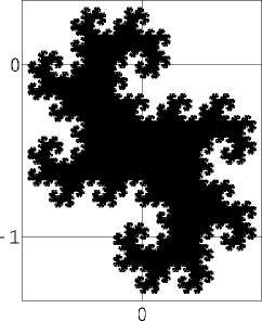
$\mathbf{T}$

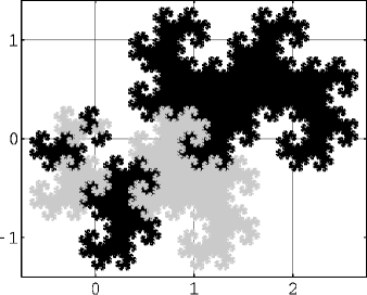
$\mathbf{N}^{2}\left(\mathbf{T}\right)$ showing action of $\mathbf{N}^{-1}$

$\mathbf{N}=\left(\begin{smallmatrix}1&-1\\ 1&1\end{smallmatrix}\right)$, $D=\left\{\left(\begin{smallmatrix}0\\ 0\end{smallmatrix}\right),\left(\begin{smallmatrix}1\\ 0\end{smallmatrix}\right)\right\}$

Figure 2. Twin-Dragon (Example 9.7)

Example 9.7.

Let $\mathbf{N}=\left(\begin{smallmatrix}1&-1\\ 1&1\end{smallmatrix}\right)$, $D=\left\{\left(\begin{smallmatrix}0\\ 0\end{smallmatrix}\right),\left(\begin{smallmatrix}1\\ 0\end{smallmatrix}\right)\right\}$. Then $\mathbf{N}^{4}=-4\hbox{\small 1\kern-3.3pt\normalsize 1}_{2}=\left(\begin{smallmatrix}-4&0\\ 0&-4\end{smallmatrix}\right)$, and $\mathbf{N}^{8}=2^{4}\hbox{\small 1\kern-3.3pt\normalsize 1}_{2}=\left(\begin{smallmatrix}16&0\\ 0&16\end{smallmatrix}\right)$; and $T\left(\mathbf{N},D\right)$ is the twin-dragon set ([Ban91], [Ban96], [DDL]) which has fractal boundary. (See Figure 2 for a sketch.) Property (ii) is illustrated in this example where $\left(\begin{smallmatrix}1\\ 0\end{smallmatrix}\right)+\mathbf{N}\left(\begin{smallmatrix}0\\ 1\end{smallmatrix}\right)=\left(\begin{smallmatrix}0\\ 1\end{smallmatrix}\right)$ and

$$D^{\prime}=D+\mathbf{N}D+\mathbf{N}^{2}D+\mathbf{N}^{3}D=\left\{\begin{pmatrix}i_{0}+i_{1}-2i_{3}\\ i_{1}+2i_{2}+2i_{3}\end{pmatrix}\biggm{|}i_{0},i_{1},i_{2},i_{3}\in\left\{0,1\right\}\right\}\text{.}$$

So we have two order-one Cuntz states given by the fixed points $\left(\begin{smallmatrix}0\\ 0\end{smallmatrix}\right)$ and $\left(\begin{smallmatrix}0\\ 1\end{smallmatrix}\right)$, and using the method of Scholium 3.9, one can show that these are all the atoms of this representation. These points can also be read off Figure 2.

A result of Knuth [Knu, p. 190, Fig. 1] may be translated into the observation that the related $\left(\mathbf{N},D\right)$-system with $\mathbf{N}=\left(\begin{smallmatrix}-1&-1\\ 1&-1\end{smallmatrix}\right)$ and $D=\left\{\left(\begin{smallmatrix}0\\ 0\end{smallmatrix}\right),\left(\begin{smallmatrix}1\\ 0\end{smallmatrix}\right)\right\}$ has just a single Cuntz state, corresponding to $\left(\begin{smallmatrix}0\\ 0\end{smallmatrix}\right)^{\sim}=\mathbb{Z}^{2}$. The effect on our present $\mathbf{T}$ in Figure 2 is an affine transformation wiping out $\left(\begin{smallmatrix}0\\ 1\end{smallmatrix}\right)$ in $B_{\infty}$, i.e., this point won’t be in the rotated $-\mathbf{T}$ from Knuth’s example.

$\mathbf{T}$

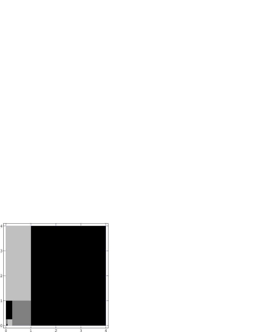
$\mathbf{N}^{2}\left(\mathbf{T}\right)$ showing action of $\mathbf{N}^{-1}$

$\mathbf{N}=\left(\begin{smallmatrix}0&1\\ 4&0\end{smallmatrix}\right)$, $D=\left\{\left(\begin{smallmatrix}0\\ 0\end{smallmatrix}\right),\left(\begin{smallmatrix}0\\ 1\end{smallmatrix}\right),\left(\begin{smallmatrix}0\\ 2\end{smallmatrix}\right),\left(\begin{smallmatrix}0\\ 3\end{smallmatrix}\right)\right\}$

Figure 3. Unit Square (Example 9.8)

Example 9.8.

$\mathbf{N}=\left(\begin{smallmatrix}0&1\\ 4&0\end{smallmatrix}\right)$, $D=\left\{\left(\begin{smallmatrix}0\\ k\end{smallmatrix}\right)\mid k=0,1,2,3\right\}$, where $\mathbf{N}^{2}=2^{2}\hbox{\small 1\kern-3.3pt\normalsize 1}_{2}=\left(\begin{smallmatrix}4&0\\ 0&4\end{smallmatrix}\right)$, and $D^{\prime}=D+\mathbf{N}D=\left\{\left(\begin{smallmatrix}i\\ j\end{smallmatrix}\right)\mid i,j\in\left\{0,1,2,3\right\}\right\}$. Here we have the non-trivial order-one Cuntz state corresponding to the solution

$$\begin{pmatrix}0\\ 3\end{pmatrix}+\mathbf{N}\begin{pmatrix}-1\\ -1\end{pmatrix}=\begin{pmatrix}-1\\ -1\end{pmatrix}\text{.}$$

The complete cycle-atom structure for this example is computed prior to (9.34) from which we see that $B_{\infty}=-\left\{\left(\begin{smallmatrix}0\\ 0\end{smallmatrix}\right),\left(\begin{smallmatrix}1\\ 1\end{smallmatrix}\right),\left(\begin{smallmatrix}1\\ 0\end{smallmatrix}\right),\left(\begin{smallmatrix}0\\ 1\end{smallmatrix}\right)\right\}$. This can also be read off the square in Figure 3.

The iteration for $\mathbf{N}^{2}=\left(\begin{smallmatrix}4&0\\ 0&4\end{smallmatrix}\right)$ separates coordinates:

$$\begin{cases}i_{0}+4i_{1}+4^{2}i_{2}+4^{3}i_{3}+\cdots\\ j_{0}+4j_{1}+4^{2}j_{2}+4^{3}j_{3}+\cdots\text{,}\end{cases}$$

and we get the following equation satisfied by the tile $\mathbf{T}=T\left(\mathbf{N},D\right)$ which is the unique compact solution to the equation:

$$4\mathbf{T}=\bigcup_{i,j}\left\{\mathbf{T}+\begin{pmatrix}i\\ j\end{pmatrix}\biggm{|}i,j\in\left\{0,1,2,3\right\}\right\}$$

meaning that $\mathbf{T}$ is the unit square in this case, i.e.,

$$\mathbf{T}=I\times I=\left\{\begin{pmatrix}x\\ y\end{pmatrix}\biggm{|}0\leq x\leq 1,0\leq y\leq 1\right\}\text{.}$$

So the boundary is not a fractal in Example 9.8.

Since, in Example 9.7,

$$\mathbf{N}\left(\mathbb{Z}^{2}\right)=\left\{\begin{pmatrix}n_{1}\\ n_{2}\end{pmatrix}\in\mathbb{Z}^{2}\biggm{|}n_{1}+n_{2}\in 2\mathbb{Z}\text{, }n_{1}-n_{2}\in 2\mathbb{Z}\right\}\text{,}$$

and, in Example 9.8,

$$\mathbf{N}\left(\mathbb{Z}^{2}\right)=\left\{\begin{pmatrix}n_{1}\\ n_{2}\end{pmatrix}\in\mathbb{Z}^{2}\biggm{|}n_{2}\in 4\mathbb{Z}\right\}\text{,}$$

the candidates we gave for the respective residue sets $D\subset\mathbb{Z}^{2}$ are easily seen to have the desired property: $d-d^{\prime}\notin\mathbf{N}\left(\mathbb{Z}^{2}\right)$ whenever $d,d^{\prime}\in D$ and $d\neq d^{\prime}$. But, more importantly, we can use our method from above in one dimension to find all the cycles and atoms for the other more complicated choices of full residue sets $D$.

In particular, Remark 9.2(iii) above shows how the calculations for $\nu=1$, following Proposition 8.4, may be used in the analysis of cycle–atom structure for Examples 9.7 and 9.8 above, and for related examples $\mathrm{s.t.\;}\mathbf{N}^{m}=p\hbox{\small 1\kern-3.3pt\normalsize 1}_{\nu}$ holds for some $m$, $p$.

9.5. Single-atom cases

In Example 9.1, the matrix $\mathbf{N}=\left(\begin{smallmatrix}2&1\\ 0&2\end{smallmatrix}\right)$ is special in that $\left(\mathbf{N}-\hbox{\small 1\kern-3.3pt\normalsize 1}\right)^{-1}\mathbf{N}$ is also an integral matrix. An application of Proposition 9.9, below, then yields the result that, for any other $D^{\prime}\subset\mathbb{Z}^{2}$ consisting of $4$ mutually $\mathbf{N}$-incongruent points, the corresponding $B^{\prime}_{\infty}$ will have no fewer than $4$ points, so there are at least $4$ equivalence classes for the corresponding $\approx^{\prime}$ relation. The same argument, applied to Example 9.7, shows that the corresponding number is $2$ there. Example 9.8 provides an illustration of a case where the points in $\mathbf{T}\cap\mathbb{Z}^{2}$ are obtained from the second iteration of (5.10) in Remark 5.5, needing both the cases $k=1$ and $k=2$.

The assertions made here about the lower bound on the set of periodic points in the respective examples follow from the following:

Proposition 9.9.

Assume that $\mathbf{N}$ is a $\nu\times\nu$ matrix with integer entries and $N=\left|\det\mathbf{N}\right|>0$. Assume that all the (complex) eigenvalues of $\mathbf{N}$ have modulus greater than one. If $D$ is a set of $N$ points in $\mathbb{Z}^{\nu}$ which are mutually incongruent modulo $\mathbf{N}\mathbb{Z}^{\nu}$, and

(9.8) $$D_{0}=\left\{d\in D\mid\smash{\left(\hbox{\small 1\kern-3.3pt\normalsize 1}-\mathbf{N}\right)^{-1}}d\in\mathbb{Z}^{\nu}\right\}$$

then the map $R$ associated with the admissible pair $\left(\mathbf{N},D\right)$ by Scholium 2.5 (or (1.9)) has exactly $\#\left(D_{0}\right)$ fixed points, so

$$\#\left(B_{\infty}\right)\geq\#\left(D_{0}\right)\text{.}$$

In particular, if $\left(\hbox{\small 1\kern-3.3pt\normalsize 1}-\mathbf{N}\right)^{-1}$ has integral entries, then

(9.9) $$\#\left(B_{\infty}\right)\geq N=\#\left(D\right)\text{.}$$

Proof.

If $d\in D$ and $x=\left(\hbox{\small 1\kern-3.3pt\normalsize 1}-\mathbf{N}\right)^{-1}d\in\mathbb{Z}^{\nu}$, then $R\left(x\right)=x$ and $x\in B_{\infty}$. As $\left(\hbox{\small 1\kern-3.3pt\normalsize 1}-\mathbf{N}\right)^{-1}$ is invertible, distinct $d$’s give rise to distinct $x$’s in this way. ∎

This raises the question of finding geometric properties of admissible pairs $\left(\mathbf{N},D\right)$ in $\nu$ dimensions $\nu\geq 2$; for example, when $\mathbf{N}$ is given, finding conditions on $D\subset\mathbb{Z}^{\nu}$ such that $\left(\mathbf{N},D\right)$ is admissible, and the corresponding $B_{\infty}=\left(-\mathbf{T}\right)\cap\mathbb{Z}^{\nu}$ is a singleton. This means that the associated representation of $\mathop{\rm UHF}\nolimits_{N}$ is irreducible on $L^{2}\left(\mathbb{T}^{\nu}\right)$.

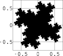
$\mathbf{T}$

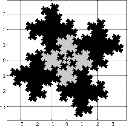
$\mathbf{N}^{2}\left(\mathbf{T}\right)$ showing action of $\mathbf{N}^{-1}$

$\mathbf{N}=\left(\begin{smallmatrix}1&2\\ -2&1\end{smallmatrix}\right)$, $D=\left\{\left(\begin{smallmatrix}0\\ 0\end{smallmatrix}\right),\left(\begin{smallmatrix}\pm 1\\ 0\end{smallmatrix}\right),\left(\begin{smallmatrix}0\\ \pm 1\end{smallmatrix}\right)\right\}$

Figure 4. Fractal Red Cross (Example 9.10)

Example 9.10.

We note that Proposition 9.9 does not apply to $\mathbf{N}=\left(\begin{smallmatrix}1&2\\ -2&1\end{smallmatrix}\right)$, as $\left(\mathbf{N}-\hbox{\small 1\kern-3.3pt\normalsize 1}\right)^{-1}\mathbf{N}=\left(\begin{smallmatrix}1&-\frac{1}{2}\\ \frac{1}{2}&1\end{smallmatrix}\right)$ does not have integer entries. Using estimates from Section 3, we now show that the answer is “yes” for $\mathbf{N}=\left(\begin{smallmatrix}1&2\\ -2&1\end{smallmatrix}\right)$, i.e., it admits $D$ with $B_{\infty}$ a singleton. There are also examples in one dimension if $N>2$, and in higher dimensions with $B_{\infty}$ a singleton. Take for example $N=3$ and $D=\left\{2k-1,2k,2k+1\right\}$ with $k\in\mathbb{Z}$; then it follows from Corollary 3.11 that $B_{\infty}=\left\{-k\right\}$. When $N=2$ it follows from Subsection 8.1 that there are no examples with $B_{\infty}$ a one-point set. There are simple examples in two dimensions when we get non-$\mathbb{Z}^{2}$-lattice points in $\mathbf{T}$ upon applying $\left(\mathbf{N}-\hbox{\small 1\kern-3.3pt\normalsize 1}\right)^{-1}$ to the vectors in $D$. One such is the “Four-Clover”, or the “Fractal Red Cross”. This version of $\mathbf{T}$ arises from the following admissible pair $\left(\mathbf{N},D\right)$:

$$\mathbf{N}=\begin{pmatrix}1&2\\ -2&1\end{pmatrix}\text{,\quad}D=\left\{\begin{pmatrix}0\\ 0\end{pmatrix},\begin{pmatrix}\pm 1\\ 0\end{pmatrix},\begin{pmatrix}0\\ \pm 1\end{pmatrix}\right\}\text{.}$$

Here $\left(\mathbf{N}-\hbox{\small 1\kern-3.3pt\normalsize 1}\right)^{-1}=\left(\begin{smallmatrix}0&-\frac{1}{2}\\ \frac{1}{2}&0\end{smallmatrix}\right)$, i.e., non-integral, and

$$\left(\mathbf{N}-\hbox{\small 1\kern-3.3pt\normalsize 1}\right)^{-1}D=\left\{\begin{pmatrix}0\\ 0\end{pmatrix},\begin{pmatrix}0\\ \pm\frac{1}{2}\end{pmatrix},\begin{pmatrix}\pm\frac{1}{2}\\ 0\end{pmatrix}\right\}\text{.}$$

In fact, it can be checked that

$$\mathbf{T}\cap\mathbb{Z}^{2}=\left\{\begin{pmatrix}0\\ 0\end{pmatrix}\right\}\text{,}$$

meaning that here we get just a single atom. In the terminology of Powers [Pow88], this means (as we recalled in Section 1) that the corresponding endomorphism of $\mathcal{B}\left(L^{2}\left(\mathbb{T}^{2}\right)\right)$ is a (Powers) shift.

To verify that $\mathbf{T}\cap\mathbb{Z}^{2}=\left\{\left(\begin{smallmatrix}0\\ 0\end{smallmatrix}\right)\right\}$, use Corollary 3.10, formula (5.9) in Remark 5.5, and the observation that $\mathbf{N}$ here is diagonalizable with eigenvalues $\lambda_{\pm}=1\pm i2$. Specifically, since $\left|\lambda_{+}\right|=\left|\lambda_{-}\right|=\sqrt{5}$, the argument from the proof of Corollary 3.11 also shows that every point $x=\left(\begin{smallmatrix}i\\ j\end{smallmatrix}\right)\in B_{\infty}=\left(-\mathbf{T}\right)\cap\mathbb{Z}^{2}$ must satisfy $\left\|x\right\|\leq\frac{1}{\sqrt{5}-1}<1$ where $\left\|x\right\|=\sqrt{i^{2}+j^{2}}$. This norm is appropriate since $\mathbf{N}=\hbox{\small 1\kern-3.3pt\normalsize 1}+\left(\begin{smallmatrix}0&2\\ -2&0\end{smallmatrix}\right)$ and $\left(\begin{smallmatrix}0&2\\ -2&0\end{smallmatrix}\right)$ is skew-adjoint, so the eigenvectors of $\mathbf{N}$ in $\mathbb{C}^{2}$ are orthogonal. It follows that $B_{\infty}=\left\{\left(\begin{smallmatrix}0\\ 0\end{smallmatrix}\right)\right\}$ as claimed. Note further that the discussion here falls within the class of ultraspecial examples in Remark 3.16 where the estimate (3.17) is in fact an equality, since $\left\|\mathbf{N}^{-1}\right\|=5^{-\frac{1}{2}}$. (The same argument, for Example 9.7 (the Twin Dragon), shows that points $x$ in $\mathbf{T}$ there must satisfy $\left\|x\right\|\leq\frac{1}{\sqrt{2}-1}$.)

A more refined construction of single-atom examples (analogous to $D_{1}$) in higher even dimensions may be based on the known Hadamard matrices from combinatorics; see, e.g., [JoPe96] and [Haa]. If $\nu$ is even, a $\nu\times\nu$ matrix $\mathbf{N}$ with entries $\pm 1$ is said to be Hadamard if $\mathbf{N}^{*}\mathbf{N}=\nu\hbox{\small 1\kern-3.3pt\normalsize 1}_{\nu}$. Then of course, the spectrum of $\mathbf{N}$ must be in $\left\{\lambda\in\mathbb{C}\mid\left|\lambda\right|=\sqrt{\nu}\right\}$ and $\left\|\mathbf{N}^{-1}\right\|=\nu^{-\frac{1}{2}}$. For the determinant, we have

$$N_{\nu}=\left|\det\mathbf{N}_{\nu}\right|=\left(\sqrt{\nu}\right)^{\nu}\text{.}$$

We shall need $\nu=8$ below, in which case $N_{8}=8^{4}=2^{12}$, and $\left\|\mathbf{N}_{8}^{-1}\right\|=\frac{1}{2\sqrt{2}}$. The case $\nu=2$, and $\mathbf{N}_{2}=\left(\begin{smallmatrix}1&1\\ 1&-1\end{smallmatrix}\right)$, is essentially our present Example 9.7, where the cardinality of $B_{\infty}$ is $2$. For $\nu=8$, we can take $\mathbf{N}=\mathbf{N}_{2}\otimes\mathbf{N}_{2}\otimes\mathbf{N}_{2}$. Now choose $D=\left\{d_{i}\in\mathbb{Z}^{8}\mid i=1,2,\dots,2^{12}\right\}$ such that the pair $\left(\mathbf{N},D\right)$ is admissible in $\mathbb{Z}^{\nu}$, and

(9.10) $$\max_{i}\left\|d_{i}\right\|<2\sqrt{2}-1\text{.}$$

Then the argument from before shows that every point $x\in\mathbf{T}=-\mathbf{T}$ must satisfy $\left\|x\right\|<1$; and therefore, by Proposition 3.12, $B_{\infty}=\left\{0\right\}$ for those examples.

It is known (see, e.g., [Haa]) that there are other higher-order Hadamard matrices than those which arise from the simple tensor construction.

We also note that the tensor construction works for matrices more general than the Hadamard matrices: if $\mathbf{N}_{i}$ are given integral matrices of size $\nu_{i}$, $i=1,2$, and if there are $p_{i}$’s $>1$, such that $\mathbf{N}^{*}_{i}\mathbf{N}_{i}=p_{i}\hbox{\small 1\kern-3.3pt\normalsize 1}_{\nu_{i}}$, then set $\mathbf{M}=\mathbf{N}_{1}\otimes\mathbf{N}_{2}$, and we will have $\mathbf{M}^{*}\mathbf{M}$ represented as a diagonal matrix which yields us the estimate $\left\|\mathbf{M}^{-1}\right\|\leq\frac{1}{\min\left(p_{1},p_{2}\right)}<1$. Therefore, if $D\subset\mathbb{Z}^{\nu_{1}\nu_{2}}$ is chosen such that $\left(\mathbf{N},D\right)$ is admissible, and also assuming

(9.11) $$\max_{j}\left\|d_{j}\right\|<\min\left(p_{1},p_{2}\right)-1\text{,}$$

then we will have an example $\left(\mathbf{M},D\right)$ in $\nu_{1}\nu_{2}$ dimensions with $B_{\infty}=\left\{0\right\}$. But the selection of the set $D$ of residues in $\nu_{1}\nu_{2}$ dimensions is easier if the individual matrices $\mathbf{N}_{i}$, $i=1,2$, are Hadamard. In the more general cases, the explicit construction of admissible residue sets in $\nu_{1}\nu_{2}$ dimensions may be difficult. In particular, the conditions (9.10) and (9.11) show that a more detailed classification of the single-atom cases must depend also on the asymptotics of the counting function

(9.12) $$N_{\nu}\left(R,a\right)=\#\left\{x\in\mathbb{Z}^{\nu}\mid\left|x-a\right|\leq R\right\}$$

where $\left|x-a\right|=\left(\sum_{i}\left(x_{i}-a_{i}\right)^{2}\right)^{\frac{1}{2}}$. Even for $\nu=2$, this is a problem of current interest; see, e.g., [BlDy].

9.6. Multiple coverings

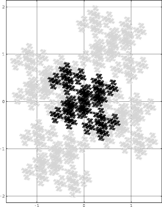
Sometimes we see a cloud that’s dragonish… (Shakespeare, Antony and Cleopatra) Shading added to illustrate how $\mathbf{T}$ is formed as a “reptile”, that is, the union of the five subtiles, the central one $\tau_{\left(\begin{smallmatrix}0\\ 0\end{smallmatrix}\right)}\left(\mathbf{T}\right)=\mathbf{N}^{-1}\mathbf{T}$ (dark), and the two pairs, $\tau_{\left(\begin{smallmatrix}\pm 3\\ 0\end{smallmatrix}\right)}\left(\mathbf{T}\right)=\pm\tau_{\left(\begin{smallmatrix}3\\ 0\end{smallmatrix}\right)}\left(\mathbf{T}\right)$ and $\tau_{\left(\begin{smallmatrix}0\\ \pm 2\end{smallmatrix}\right)}\left(\mathbf{T}\right)=\pm\tau_{\left(\begin{smallmatrix}0\\ 2\end{smallmatrix}\right)}\left(\mathbf{T}\right)$ in symmetry (light), with respective interiors of distinct subtiles non-overlapping, i.e., “just-touching” subtiles. $\mathbf{N}=\left(\begin{smallmatrix}1&2\\ -2&1\end{smallmatrix}\right)$, $D=\left\{\left(\begin{smallmatrix}0\\ 0\end{smallmatrix}\right),\left(\begin{smallmatrix}\pm 3\\ 0\end{smallmatrix}\right),\left(\begin{smallmatrix}0\\ \pm 2\end{smallmatrix}\right)\right\}$

Figure 5. Cloud Nine (Example 9.11)

The single-atom case is relevant to, among other things, the complex-base problem [Gil]. See Remark 3.14, where we also noted that the single-atom case makes the corresponding $\mathbf{T}$ tile $\mathbb{R}^{\nu}$ by the unit lattice $\mathbb{Z}^{\nu}$. We now turn to the case where $B_{\infty}$ is not a singleton, but where we still retain the lattice geometry for $\mathbf{T}$. Then we will expect $\mathbf{T}$ to tile $\mathbb{R}^{\nu}$ with a proper sublattice $\mathbb{L\kern 0.5pt}\subset\mathbb{Z}^{\nu}$, and, hence, $\mathbf{T}$ will be a finite covering. When $\mathbf{N}=\left(\begin{smallmatrix}1&2\\ -2&1\end{smallmatrix}\right)$, the associated fractal $\mathbf{T}=\mathbf{T}\left(D\right)$ can easily be computed for the following candidates for $D$:

(9.13) $$D_{1} =\left\{\begin{pmatrix}0\\ 0\end{pmatrix},\begin{pmatrix}\pm 1\\ 0\end{pmatrix},\begin{pmatrix}0\\ \pm 1\end{pmatrix}\right\}$$  (Fractal Red Cross, Fig. 4)

$$D_{9} =\left\{\begin{pmatrix}0\\ 0\end{pmatrix},\begin{pmatrix}\pm 3\\ 0\end{pmatrix},\begin{pmatrix}0\\ \pm 2\end{pmatrix}\right\}$$  (Cloud Nine, Fig. 5)

$$D_{3} =\left\{\begin{pmatrix}0\\ 0\end{pmatrix},\begin{pmatrix}0\\ \pm 1\end{pmatrix},\begin{pmatrix}0\\ \pm 2\end{pmatrix}\right\}$$  (Cloud Three, Fig. 7)

$$D_{5} =\left\{\begin{pmatrix}0\\ 0\end{pmatrix},\begin{pmatrix}\pm 3\\ 0\end{pmatrix},\begin{pmatrix}\pm 1\\ 0\end{pmatrix}\right\}$$  (Cloud Five, Fig. 8)

Example 9.11.

Choosing, for example, $D_{9}=\left\{\left(\begin{smallmatrix}0\\ 0\end{smallmatrix}\right),\left(\begin{smallmatrix}\pm 3\\ 0\end{smallmatrix}\right),\left(\begin{smallmatrix}0\\ \pm 2\end{smallmatrix}\right)\right\}$, gets us two fixed points $\left(\begin{smallmatrix}\pm 1\\ 0\end{smallmatrix}\right)$ in $B^{(9)}_{\infty}$ in addition to the one point in $B_{\infty}=\left\{\left(\begin{smallmatrix}0\\ 0\end{smallmatrix}\right)\right\}$ for the other choice of $D=\left\{\left(\begin{smallmatrix}0\\ 0\end{smallmatrix}\right),\left(\begin{smallmatrix}\pm 1\\ 0\end{smallmatrix}\right),\left(\begin{smallmatrix}0\\ \pm 1\end{smallmatrix}\right)\right\}$. More specifically, there are nine points in the set $B^{(9)}_{\infty}=\left(-\mathbf{T}_{9}\right)\cap\mathbb{Z}^{2}=\left\{\left(\begin{smallmatrix}0\\ 0\end{smallmatrix}\right),\left(\begin{smallmatrix}\pm 1\\ 0\end{smallmatrix}\right),\left(\begin{smallmatrix}0\\ \pm 1\end{smallmatrix}\right),\left(\begin{smallmatrix}\pm 1\\ \pm 1\end{smallmatrix}\right)\right\}$ (see Figure 5). We still have the symmetry $\mathbf{T}_{9}=-\mathbf{T}_{9}$ when $\mathbf{T}_{9}$ is determined from (3.11) corresponding to $D_{9}$, and we have displayed both $\mathbf{T}_{1}$ and $\mathbf{T}_{9}$ in Figures 4 and 5. We now prove the assertion about $B^{(9)}_{\infty}$ “the hard way” (as opposed to “merely” reading the picture). First the argument from Example 9.1 shows that $R^{\prime n}\left(x\right)$ is eventually contained in the euclidean sphere of radius

$$\frac{3}{\sqrt{5}}\left(\vphantom{\sum\left(\frac{1}{\sqrt{5}}\right)^{n}}\smash{\sum_{n=0}^{\infty}\left(\frac{1}{\sqrt{5}}\right)^{n}}\right)=\frac{3}{\sqrt{5}-1}=2.427\dots$$

regardless of which starting point $x$ in $\mathbb{Z}^{2}$ is chosen. Here we use the notation $R^{\prime}$ for the mapping given by (1.9) with $D_{9}=\left\{\left(\begin{smallmatrix}0\\ 0\end{smallmatrix}\right),\left(\begin{smallmatrix}\pm 3\\ 0\end{smallmatrix}\right),\left(\begin{smallmatrix}0\\ \pm 2\end{smallmatrix}\right)\right\}$, and it is immediate that $R^{\prime}\left(\begin{smallmatrix}0\\ 0\end{smallmatrix}\right)=\left(\begin{smallmatrix}0\\ 0\end{smallmatrix}\right)$, $R^{\prime}\left(\begin{smallmatrix}\pm 1\\ 0\end{smallmatrix}\right)=\left(\begin{smallmatrix}\pm 1\\ 0\end{smallmatrix}\right)$; i.e., three points of period one. A direct calculation, as in Example 9.1 above, also yields

$$\begin{pmatrix}0\\ 1\end{pmatrix}\overset{\raise 1.0pt\hbox{$\scriptstyle R^{\prime}$}}{\rightarrow}\begin{pmatrix}-1\\ -1\end{pmatrix}\overset{\raise 1.0pt\hbox{$\scriptstyle R^{\prime}$}}{\rightarrow}\begin{pmatrix}1\\ -1\end{pmatrix}\overset{\raise 1.0pt\hbox{$\scriptstyle R^{\prime}$}}{\rightarrow}\begin{pmatrix}0\\ -1\end{pmatrix}\overset{\raise 1.0pt\hbox{$\scriptstyle R^{\prime}$}}{\rightarrow}\begin{pmatrix}1\\ 1\end{pmatrix}\overset{\raise 1.0pt\hbox{$\scriptstyle R^{\prime}$}}{\rightarrow}\begin{pmatrix}-1\\ 1\end{pmatrix}\overset{\raise 1.0pt\hbox{$\scriptstyle R^{\prime}$}}{\rightarrow}\begin{pmatrix}0\\ 1\end{pmatrix}$$

(see also Figure 6), and thus,

$$\left(R^{\prime}\right)^{6}\begin{pmatrix}0\\ 1\end{pmatrix}=\begin{pmatrix}0\\ 1\end{pmatrix}\text{.}$$

Hence the point $\left(\begin{smallmatrix}0\\ 1\end{smallmatrix}\right)$ has (minimal) period equal to $6$.

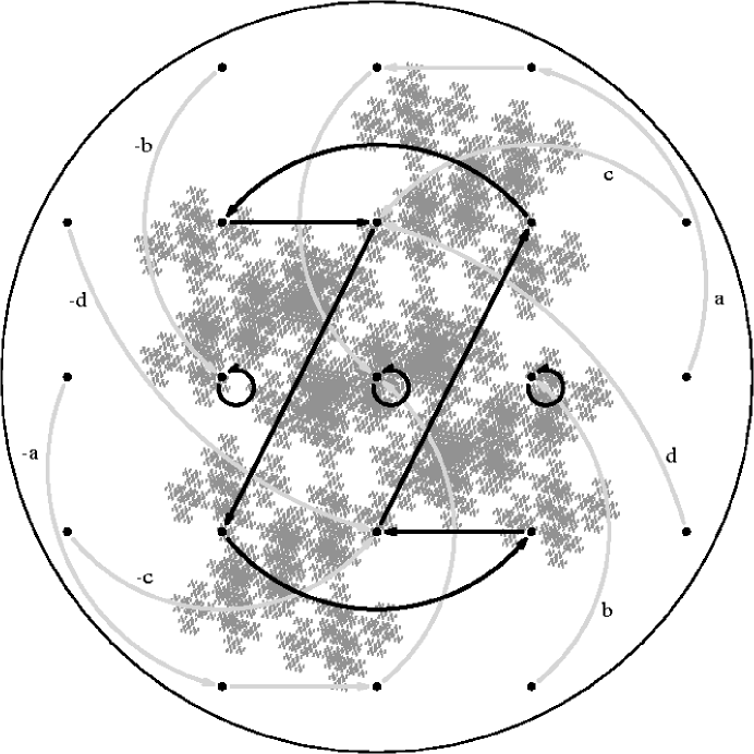
Figure 6. Paths of points within spectral circle for Cloud Nine (Example 9.11)

Furthermore, we can check directly that the additional points within the spectral circle have the following paths:

($$\mathrm{a} \begin{pmatrix}2\\ 0\end{pmatrix}\overset{\raise 1.0pt\hbox{$\scriptstyle R^{\prime}$}}{\rightarrow}\begin{pmatrix}1\\ 2\end{pmatrix}\overset{\raise 1.0pt\hbox{$\scriptstyle R^{\prime}$}}{\rightarrow}\begin{pmatrix}0\\ 2\end{pmatrix}\overset{\raise 1.0pt\hbox{$\scriptstyle R^{\prime}$}}{\rightarrow}\begin{pmatrix}0\\ 0\end{pmatrix}\text{,}$$)

($$-\mathrm{a} \begin{pmatrix}-2\\ 0\end{pmatrix}\overset{\raise 1.0pt\hbox{$\scriptstyle R^{\prime}$}}{\rightarrow}\begin{pmatrix}-1\\ -2\end{pmatrix}\overset{\raise 1.0pt\hbox{$\scriptstyle R^{\prime}$}}{\rightarrow}\begin{pmatrix}0\\ -2\end{pmatrix}\overset{\raise 1.0pt\hbox{$\scriptstyle R^{\prime}$}}{\rightarrow}\begin{pmatrix}0\\ 0\end{pmatrix}\text{,}$$)

($$\mathrm{b} \begin{pmatrix}1\\ -2\end{pmatrix}\overset{\raise 1.0pt\hbox{$\scriptstyle R^{\prime}$}}{\rightarrow}\begin{pmatrix}1\\ 0\end{pmatrix}\overset{\raise 1.0pt\hbox{$\scriptstyle R^{\prime}$}}{\rightarrow}\begin{pmatrix}1\\ 0\end{pmatrix}\text{,}$$)

($$-\mathrm{b} \begin{pmatrix}-1\\ 2\end{pmatrix}\overset{\raise 1.0pt\hbox{$\scriptstyle R^{\prime}$}}{\rightarrow}\begin{pmatrix}-1\\ 0\end{pmatrix}\overset{\raise 1.0pt\hbox{$\scriptstyle R^{\prime}$}}{\rightarrow}\begin{pmatrix}-1\\ 0\end{pmatrix}\text{,}$$)

($$\mathrm{c} \begin{pmatrix}2\\ 1\end{pmatrix}\overset{\raise 1.0pt\hbox{$\scriptstyle R^{\prime}$}}{\rightarrow}\begin{pmatrix}0\\ 1\end{pmatrix}\overset{\raise 1.0pt\hbox{$\scriptstyle R^{\prime}$}}{\rightarrow}6\text{-cycle,}$$)

($$-\mathrm{c} \begin{pmatrix}-2\\ -1\end{pmatrix}\overset{\raise 1.0pt\hbox{$\scriptstyle R^{\prime}$}}{\rightarrow}\begin{pmatrix}0\\ -1\end{pmatrix}\overset{\raise 1.0pt\hbox{$\scriptstyle R^{\prime}$}}{\rightarrow}6\text{-cycle,}$$)

($$\mathrm{d} \begin{pmatrix}2\\ -1\end{pmatrix}\overset{\raise 1.0pt\hbox{$\scriptstyle R^{\prime}$}}{\rightarrow}\begin{pmatrix}0\\ 1\end{pmatrix}\overset{\raise 1.0pt\hbox{$\scriptstyle R^{\prime}$}}{\rightarrow}6\text{-cycle,}$$)

($$-\mathrm{d} \begin{pmatrix}-2\\ 1\end{pmatrix}\overset{\raise 1.0pt\hbox{$\scriptstyle R^{\prime}$}}{\rightarrow}\begin{pmatrix}0\\ -1\end{pmatrix}\overset{\raise 1.0pt\hbox{$\scriptstyle R^{\prime}$}}{\rightarrow}6\text{-cycle.}$$)

The flow diagram illustrates the fact that some points in the pattern are stable points of attraction in the sense of [LiMa].

Hence we have all $21$ points in the spectral circle covered: three have period $1$, six period $6$, and the other twelve are not periodic. (See Figure 6.) Thus, of the $21$ $\mathbb{Z}^{2}$-points inside the spectral circle with radius $r=\frac{3}{\sqrt{5}-1}$, $9$ are in $B^{(9)}_{\infty}$: three single-atom cycles on the $x$-axis, and one six-atom cycle (Z-shaped). All of the three single-atom cycles have flow paths linking up to them and tracing a portion of the points inside the circle (paths $(\mathrm{a})$–$(\mathrm{b})$ in Figure 6.) Two of the six atoms in the $6$-cycle attract separate flow lines from respective points inside the circle (paths $(\mathrm{c})$–$(\mathrm{d})$ in Figure 6), and an inspection shows that all $21$ points are thus accounted for. We have described all the interior flow paths, and we note the reflection symmetry of paths under $\left(\begin{smallmatrix}x\\ y\end{smallmatrix}\right)\mapsto\left(\begin{smallmatrix}-x\\ -y\end{smallmatrix}\right)$.

Proposition 9.12.

Cloud Nine $(\mathbf{T}_{9})$ tiles $\mathbb{R}^{2}$ by the lattice $\mathbb{L\kern 0.5pt}=\mathbb{Z}\left[\left(\begin{smallmatrix}1\\ 0\end{smallmatrix}\right),\left(\begin{smallmatrix}0\\ 2\end{smallmatrix}\right)\right]$.

Proof.

In the Observation after Lemma 9.6, we consider the equivalence class $\left(\begin{smallmatrix}0\\ 0\end{smallmatrix}\right)^{\sim}$ where $\sim$ is the $\mathcal{O}_{5}$-equivalence relation determined on $\mathbb{Z}^{2}$ in Section 3 from $\mathbf{N}$ and $D_{9}=\pm\left\{\left(\begin{smallmatrix}0\\ 0\end{smallmatrix}\right),\left(\begin{smallmatrix}3\\ 0\end{smallmatrix}\right),\left(\begin{smallmatrix}0\\ 2\end{smallmatrix}\right)\right\}$. We noted after Lemma 9.6 that $\left(\begin{smallmatrix}0\\ 0\end{smallmatrix}\right)^{\sim}$ is not a lattice. For example, from path ($\mathrm{a}$) in Figure 6, note that the two points $\left(\begin{smallmatrix}1\\ 2\end{smallmatrix}\right)$ and $\left(\begin{smallmatrix}2\\ 0\end{smallmatrix}\right)$ are in $\left(\begin{smallmatrix}0\\ 0\end{smallmatrix}\right)^{\sim}$, but their sum $\left(\begin{smallmatrix}3\\ 2\end{smallmatrix}\right)$ is not. In fact, $\left(\begin{smallmatrix}3\\ 2\end{smallmatrix}\right)\in\left(\begin{smallmatrix}-1\\ 0\end{smallmatrix}\right)^{\sim}$, as follows from the extended path ($-\mathrm{b}$), $\left(\begin{smallmatrix}3\\ 2\end{smallmatrix}\right)\overset{\raise 1.0pt\hbox{$\scriptstyle R^{\prime}$}}{\rightarrow}\left(\begin{smallmatrix}-1\\ 2\end{smallmatrix}\right)\overset{\raise 1.0pt\hbox{$\scriptstyle R^{\prime}$}}{\rightarrow}\left(\begin{smallmatrix}-1\\ 0\end{smallmatrix}\right)$. We claim that

(9.14) $$\begin{pmatrix}0\\ 0\end{pmatrix}^{\sim}\cup\begin{pmatrix}1\\ 0\end{pmatrix}^{\sim}\cup\begin{pmatrix}-1\\ 0\end{pmatrix}^{\sim}=\mathbb{L\kern 0.5pt}$$

where $\mathbb{L\kern 0.5pt}$ is the lattice $\mathbb{L\kern 0.5pt}=\left\{\left(\begin{smallmatrix}m\\ 2n\end{smallmatrix}\right)\mid m,n\in\mathbb{Z}\right\}$. It is clear from an inspection that the three equivalence classes are contained in $\mathbb{L\kern 0.5pt}$, and an induction argument shows that we get all of $\mathbb{L\kern 0.5pt}$ as a disjoint union of the three $\sim$-classes, proving (9.14). Recall that the three points $\left(\begin{smallmatrix}0\\ 0\end{smallmatrix}\right)$ and $\left(\begin{smallmatrix}\pm 1\\ 0\end{smallmatrix}\right)$ are precisely the solutions $x$ in $\mathbb{Z}^{2}$ to $R^{\prime}x=x$, i.e., the points in $B^{(9)}_{\infty}$ of period one. Using now (9.14) in place of the corresponding condition in Lemma 9.6 above, we conclude that $\mathbf{T}_{9}$ tiles $\mathbb{R}^{2}$ by the lattice $\mathbb{L\kern 0.5pt}$ as claimed. We omit details, but they are essentially in the proof of Lemma 9.6. ∎

Remark 9.13.

The proof also suggests a possible general scheme for getting lattices $\mathbb{L\kern 0.5pt}$ associated with given “reptiles” $\mathbf{T}$ in $\mathbb{R}^{\nu}$, i.e., the (3.11) ones. Given $\left(\mathbf{N},D\right)$ in $\nu$ dimensions with $0\in D$, and specified as in Section 3, then introduce $R$, the equivalence relation $\sim$, and the corresponding set $B_{\infty}$ of periodic points. Then look for minimal subsets $P$ of $B_{\infty}$ containing $0$ such that $\bigcup_{p\in P}p^{\sim}$ is a rank-$\nu$ lattice $\mathbb{L\kern 0.5pt}\subset\mathbb{Z}^{\nu}$, and show that $\mathbf{T}$ tiles $\mathbb{R}^{\nu}$ by $\mathbb{L\kern 0.5pt}$.

The Fractal Red Cross is graphed in Figure 4 and discussed in [Str94], and its boundary is fractal in a sense which is specified there; its scaling similarity dimension is $d_{s}=\frac{2\ln 3}{\ln 5}$. We note that the boundaries of $\mathbf{T}$ for our Examples 9.1 and 9.7 are also fractal. In Figure 1, for example, the boundary consists of two intervals, and the rest is fractal. (See also [Ban96].) While the extent of the overlap in $\mathbf{T}=\bigcup_{d\in D}\mathbf{N}^{-1}\left(d+\mathbf{T}\right)$ from (3.11) isn’t quite clear in Example 9.11 (Figure 5), there is some overlap which can be entered into the formula used for the similarity scaling dimension $d_{s}$ of $\partial\mathbf{T}$ for Example 9.10. If the relative overlap is specified by a fraction $0<\beta<1$, then the scaling dimension is $\frac{2\ln\left(3+\beta\right)}{\ln 5}$ by the Strichartz argument used in Example 9.10.

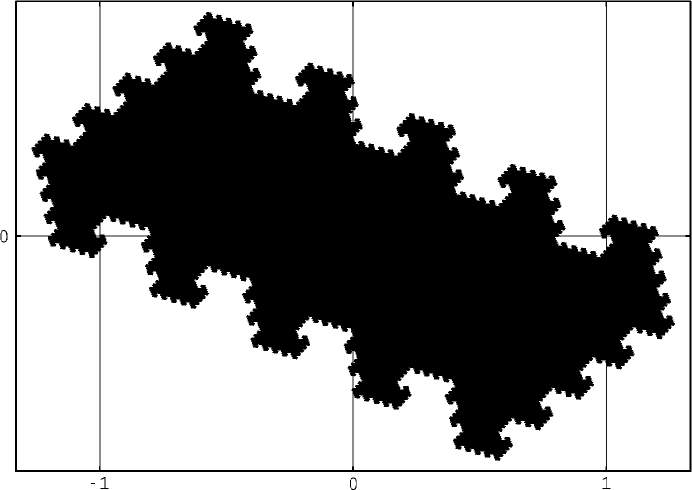
$\mathbf{N}=\left(\begin{smallmatrix}1&2\\ -2&1\end{smallmatrix}\right)$, $D=\left\{\left(\begin{smallmatrix}0\\ 0\end{smallmatrix}\right),\left(\begin{smallmatrix}0\\ \pm 1\end{smallmatrix}\right),\left(\begin{smallmatrix}0\\ \pm 2\end{smallmatrix}\right)\right\}$

Figure 7. Cloud Three (Example 9.14)

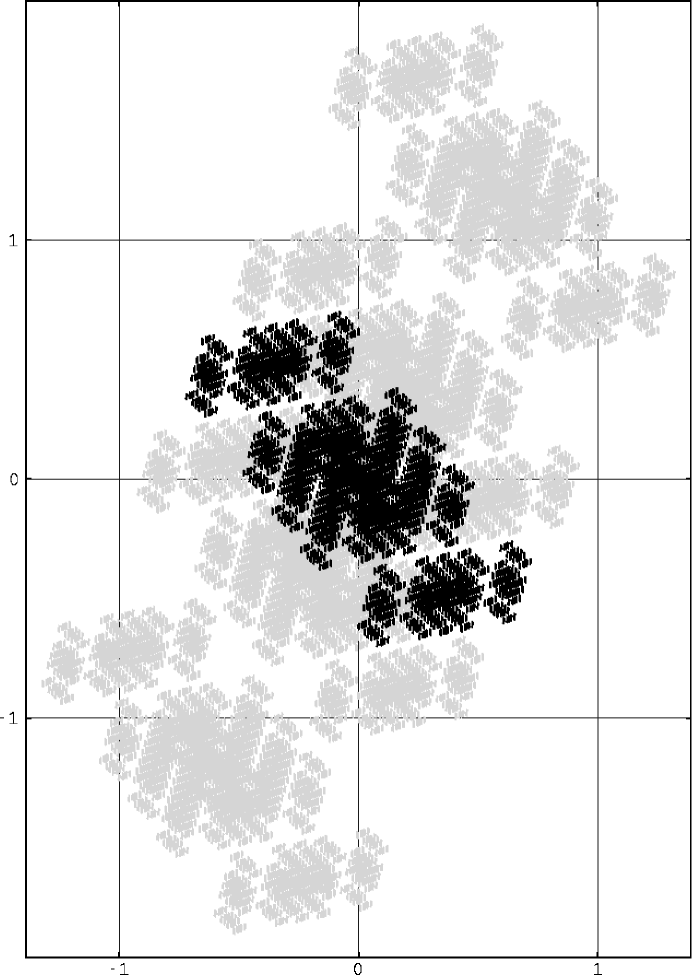
We use the same shading convention here as in Figure 5. $\mathbf{N}=\left(\begin{smallmatrix}1&2\\ -2&1\end{smallmatrix}\right)$, $D=\left\{\left(\begin{smallmatrix}0\\ 0\end{smallmatrix}\right),\left(\begin{smallmatrix}\pm 3\\ 0\end{smallmatrix}\right),\left(\begin{smallmatrix}\pm 1\\ 0\end{smallmatrix}\right)\right\}$

Figure 8. Cloud Five (Example 9.14)

Example 9.14.

A simpler version of the fractal $\mathbf{T}_{9}$ derives from taking $D_{3}=\left\{\left(\begin{smallmatrix}0\\ 0\end{smallmatrix}\right),\left(\begin{smallmatrix}0\\ \pm 1\end{smallmatrix}\right),\left(\begin{smallmatrix}0\\ \pm 2\end{smallmatrix}\right)\right\}$, still with $\mathbf{N}=\left(\begin{smallmatrix}1&2\\ -2&1\end{smallmatrix}\right)$. Then $B^{(3)}_{\infty}=\left\{\left(\begin{smallmatrix}0\\ 0\end{smallmatrix}\right),\left(\begin{smallmatrix}\pm 1\\ 0\end{smallmatrix}\right)\right\}$, and there are three cycles each with one atom. $\mathbf{T}$ is then as in Figure 7.

It follows from a theorem of Lagarias and Wang [LaWa2] that when $\mathbf{N}=\left(\begin{smallmatrix}1&2\\ -2&1\end{smallmatrix}\right)$, and $D\subset\mathbb{Z}^{2}$ is chosen as a full set of residues for $\mathbb{Z}^{2}\diagup\mathbf{N}\mathbb{Z}^{2}$, then the corresponding fractal $\mathbf{T}=\mathbf{T}\left(D\right)$ is a $\mathbb{Z}^{2}$-periodic tile iff $\mathbb{Z}\left(\mathbf{N},D\right)=\mathbb{Z}^{2}$ where $\mathbb{Z}\left(\mathbf{N},D\right)$ is the smallest $\mathbf{N}$-invariant lattice containing $\left\{d-d^{\prime}\mid d,d^{\prime}\in D\right\}$. The examples with $D=D_{i}$ as given in (9.13) represent the first four cases in a double-indexed family of examples: $\mathbf{N}=\left(\begin{smallmatrix}1&2\\ -2&1\end{smallmatrix}\right)$, and $D\left(p,q\right)=\mathbf{M}\left(p,q\right)\left(D_{1}\right)$, a full set of residues, where the matrix $\mathbf{M}$ is

(9.15) $$\mathbf{M}\left(p,q\right)=\begin{pmatrix}1-p&3q\\ 2p&1-q\end{pmatrix}\text{,}$$

and $\left(p,q\right)\in\mathbb{Z}^{2}$. The numbers of elements in the corresponding sets $B_{\infty}$ of periodic points are $1$, $9$, $3$, and $5$, respectively. By checking $\mathbb{Z}\left(\mathbf{N},D_{i}\right)$, and using the Lagarias-Wang theorem, we note that, of the four fractals $\mathbf{T}_{i}$, $i=1,9,3$, and $5$, only $\mathbf{T}_{1}$ (Fractal Red Cross) is a $\mathbb{Z}^{2}$-tile, i.e., it is the only one of the four which is a periodic tile of $\mathbb{R}^{2}$ by $\mathbb{Z}^{2}$. Specifically, $\left(\begin{smallmatrix}1\\ 0\end{smallmatrix}\right)\notin\mathbb{Z}\left(\mathbf{N},D_{3}\right)$, and the point $\left(\begin{smallmatrix}0\\ 1\end{smallmatrix}\right)$ is not in either of the two lattices $\mathbb{Z}\left(\mathbf{N},D_{5}\right)$ or $\mathbb{Z}\left(\mathbf{N},D_{9}\right)$. The scaling self-similarity dimensions of the respective boundaries $\partial\mathbf{T}_{i}$ also vary from one to the next. (The graph of $\mathbf{T}_{5}$ is shown in Figure 8.)

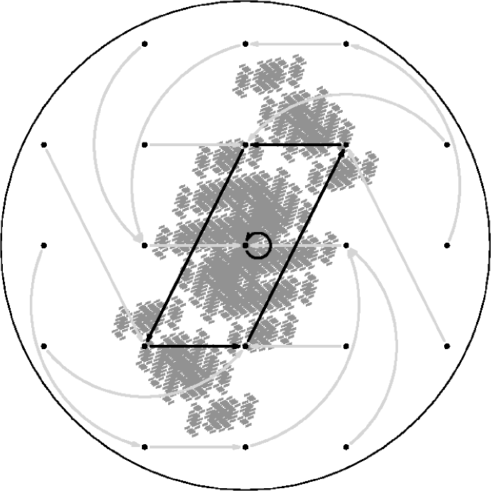
Figure 9. Paths of points within spectral circle for Cloud Five (Example 9.14)

All four $D_{i}$’s have been selected such that $0\in D_{i}$, and $D_{i}=-D_{i}$. As a result, $0\in\mathbf{T}_{i}$, and $\mathbf{T}_{i}=-\mathbf{T}_{i}$, with the point $0$ making a single-atom cycle $\left\{\left(\begin{smallmatrix}0\\ 0\end{smallmatrix}\right)\right\}$. For the two corresponding to $i=5$ and $9$, we have higher-order cycles in $B^{(i)}_{\infty}=\mathbf{T}_{i}\cap\mathbb{Z}^{2}$, and they surround the single-atom cycle $\left\{\left(\begin{smallmatrix}0\\ 0\end{smallmatrix}\right)\right\}$ with winding number one. The higher-order closed cycles have the respective orders $6$, for $\mathbf{T}_{9}$, as computed in Example 9.11 (Cloud Nine, cf. Figure 6), and $4$ for $\mathbf{T}_{5}$ (Cloud Five, cf. Figure 9). Let us look closer at $\mathbf{T}_{5}$, and repeat the analysis in Example 9.11. There are $21$ $\mathbb{Z}^{2}$-points inside the spectral circle with radius $r=\frac{3}{\sqrt{5}-1}$, and, of these, $5$ are in $B_{\infty}^{(5)}$: one single-atom cycle at the origin $0$, and the parallelogram-shaped four-atom cycle

$$\begin{pmatrix}1\\ 1\end{pmatrix}\rightarrow\begin{pmatrix}0\\ 1\end{pmatrix}\rightarrow\begin{pmatrix}-1\\ -1\end{pmatrix}\rightarrow\begin{pmatrix}0\\ -1\end{pmatrix}\rightarrow\begin{pmatrix}1\\ 1\end{pmatrix}\text{.}$$

The single-atom cycle $0$ has multiple flow paths from points inside the circle, and linking up at $0$. All four atoms in the $4$-cycle similarly attract flow paths from respective points inside (and outside) the circle, and an inspection shows that all $21$ points are accounted for. We have described the following flow paths for Cloud Five (inside the circle) (see Figure 9):

$$\begin{pmatrix}1\\ -2\end{pmatrix}\rightarrow\begin{pmatrix}1\\ 0\end{pmatrix}\rightarrow\begin{pmatrix}0\\ 0\end{pmatrix}\text{,}$$

$$\begin{pmatrix}2\\ 0\end{pmatrix}\rightarrow\begin{pmatrix}1\\ 2\end{pmatrix}\rightarrow\begin{pmatrix}0\\ 2\end{pmatrix}\rightarrow\begin{pmatrix}-1\\ 0\end{pmatrix}\rightarrow\begin{pmatrix}0\\ 0\end{pmatrix}\text{,}$$

$$\begin{pmatrix}1\\ -1\end{pmatrix}\rightarrow\begin{pmatrix}0\\ -1\end{pmatrix}\text{,}$$

$$\begin{pmatrix}2\\ -1\end{pmatrix}\rightarrow\begin{pmatrix}1\\ 1\end{pmatrix}\text{,}$$

$$\begin{pmatrix}2\\ 1\end{pmatrix}\rightarrow\begin{pmatrix}0\\ 1\end{pmatrix}\text{,}$$

and in addition we also have the reflected paths under $\left(\begin{smallmatrix}x\\ y\end{smallmatrix}\right)\mapsto\left(\begin{smallmatrix}-x\\ -y\end{smallmatrix}\right)$.

We have instances here in $2$ dimensions where $\mathbf{N}$ is fixed, but different choices of full residue sets $D_{i}\subset\mathbb{Z}$, $i=1,3,5,9$ result in dynamical systems $\left(\mathbb{Z}^{2},R_{i}\right)$ which are mutually non-conjugate. This follows from the fact (see [LiMa]) that the counting of periodic points for a dynamical system is a conjugacy invariant, i.e., the numbers $\#\left\{x\in X\mid R^{n}\left(x\right)=x\right\}$ when some system $R:X\rightarrow X$ is given. In one dimension, such non-conjugate examples abound; see, e.g., Subsection 8.1 above.

Note that the Lagarias-Wang theorem ([LaWa2], [LaWa1]) based on $\mathbb{Z}\left(\mathbf{N},D\right)$ does not apply to $\mathbf{N}=\left(\begin{smallmatrix}2&1\\ 0&2\end{smallmatrix}\right)$ in Example 9.1 (Figure 1) or to $\mathbf{N}=\left(\begin{smallmatrix}0&1\\ 4&0\end{smallmatrix}\right)$ in Example 9.8 (Figure 3) because the determinant there is not a prime. On the other hand, it is known [Str94] that the $\mathbf{T}$’s for those examples are in fact $\mathbb{Z}^{2}$-tiles of the plane. But the story for $\mathbf{N}=\left(\begin{smallmatrix}2&1\\ 0&2\end{smallmatrix}\right)$ is completely different if $D$ from Example 9.1 is changed to $D^{\prime}:=\left\{\left(\begin{smallmatrix}0\\ 0\end{smallmatrix}\right),\left(\begin{smallmatrix}3\\ 0\end{smallmatrix}\right),\left(\begin{smallmatrix}0\\ 1\end{smallmatrix}\right),\left(\begin{smallmatrix}3\\ 1\end{smallmatrix}\right)\right\}$. Then the corresponding $\mathbf{T}\left(D^{\prime}\right)$ does not tile with $\mathbb{Z}^{2}$, although we do have $\mathbb{Z}\left(\mathbf{N},D^{\prime}\right)=\mathbb{Z}^{2}$ for that case; see also [LaWa2] and [GrMa]. A digit set $D^{\prime}$ such that $\mathbb{Z}\left(\mathbf{N},D^{\prime}\right)=\mathbb{Z}^{2}$ is called primitive. The $D$ from Example 9.1 is also primitive, but the Shark-Jawed Parallelogram $\mathbf{T}\left(D\right)$ is a $\mathbb{Z}^{2}$-tile.

For the present examples with $\mathbf{N}=\left(\begin{smallmatrix}1&2\\ -2&1\end{smallmatrix}\right)$ and $D_{9}$, $D_{3}$, $D_{5}$ (i.e., non-primitive cases), it can be checked that the corresponding fractal $\mathbf{T}_{3}$ is a tile for the lattice $\mathbb{Z}\left(\mathbf{N},D_{3}\right)=\mathbb{Z}\left[\left(\begin{smallmatrix}2\\ 0\end{smallmatrix}\right),\left(\begin{smallmatrix}0\\ 1\end{smallmatrix}\right)\right]$ which is strictly contained in $\mathbb{Z}^{2}$. So $\mathbf{T}_{3}$ is still periodic, but not with $\mathbb{Z}^{2}$. We have $\mathbb{Z}\left(\mathbf{N},D_{3}\right)=\mathbb{Z}\left[\left(\begin{smallmatrix}2\\ 0\end{smallmatrix}\right),\left(\begin{smallmatrix}0\\ 1\end{smallmatrix}\right)\right]$ (agreeing with Figure 7), whereas $\mathbb{Z}\left(\mathbf{N},D_{5}\right)=\mathbb{Z}\left[\left(\begin{smallmatrix}1\\ 0\end{smallmatrix}\right),\left(\begin{smallmatrix}0\\ 2\end{smallmatrix}\right)\right]$ (see Figure 8). It then follows that both $\mathbf{T}_{3}$ and $\mathbf{T}_{5}$ have Lebesgue measure two. It is known from [Ban91] that the boundary for all $\mathbf{T}$’s has planar Lebesgue measure zero.

The present “cloud” examples are the first cases of an infinite two-parameter family, analogous to the one-parameter family in Subsection 8.1. For $\left(p,q\right)\in\mathbb{Z}^{2}$, set

(9.16) $$D\left(p,q\right):=\left\{\begin{pmatrix}0\\ 0\end{pmatrix},\pm\begin{pmatrix}1-p\\ 2p\end{pmatrix},\pm\begin{pmatrix}3q\\ 1-q\end{pmatrix}\right\}\text{.}$$

Let the matrix $\mathbf{N}=\left(\begin{smallmatrix}1&2\\ -2&1\end{smallmatrix}\right)$ be fixed. We then get an example for each value of $\left(p,q\right)\in\mathbb{Z}^{2}$, with $\left(0,0\right)$ corresponding to $D_{1}$, $\left(1,0\right)$ to $D_{3}$, $\left(0,1\right)$ to $D_{5}$, and $\left(p,q\right)=\left(1,1\right)$ to $D_{9}$. The cycle-atom structure for these examples in $\mathbb{Z}^{2}$ is more complicated than that for the Subsection-8.1 examples, where $D\left(p\right)=\left\{0,p\right\}$, $p\in\mathbb{N}_{odd}$, and

$$B_{\infty}\left(p\right)=-\left\{0,1,\dots,p\right\}\longleftrightarrow\mathbb{Z}\diagup p\mathbb{Z}\text{;}$$

cf. Remark 8.3. For the present examples, there is not a simple analogue of this; but we can say something about the fixed points

$$B_{\infty}^{1}\left(p,q\right)=\left\{x\in B_{\infty}\left(p,q\right)\mid R_{p,q}\left(x\right)=x\right\}$$

where $R=R_{p,q}$ is the $\mathbb{Z}^{2}$-transformation from (1.9) associated with $\left(\mathbf{N},D\left(p,q\right)\right)$:

1. If $p$ is even, then $B_{\infty}^{1}\left(p,q\right)=\left\{\left(\begin{smallmatrix}0\\ 0\end{smallmatrix}\right)\right\}$, and so this accounts for the period-one structure of examples $D_{1}$ and $D_{5}$.

2. If $p=2n+1$ $\left(n\in\mathbb{Z}\right)$, i.e., $p$ odd, then $B_{\infty}^{1}\left(p,q\right)=\left\{\left(\begin{smallmatrix}0\\ 0\end{smallmatrix}\right),\pm\left(\begin{smallmatrix}2n+1\\ n\end{smallmatrix}\right)\right\}$, and this accounts for the three fixed points for each of the examples $D_{3}$ and $D_{9}$.

To see this, let $E=\left\{\left(\begin{smallmatrix}\alpha\\ \beta\end{smallmatrix}\right)\mid\alpha,\beta\in\left\{0,\pm 1\right\},\alpha\cdot\beta=0\right\}=D_{1}$. It follows from Section 3 that $x\in B_{\infty}^{1}\left(p,q\right)$ iff, for some $\varepsilon\in E$, $x=\left(\hbox{\small 1\kern-3.3pt\normalsize 1}-\mathbf{N}\right)^{-1}\mathbf{M}\varepsilon\in\mathbb{Z}^{2}$ where $\mathbf{M}=\left(\begin{smallmatrix}1-p&3q\\ 2p&1-q\end{smallmatrix}\right)$. Indeed, writing $\varepsilon=\left(\begin{smallmatrix}\alpha\\ \beta\end{smallmatrix}\right)$, we get

$$x=\left(\hbox{\small 1\kern-3.3pt\normalsize 1}-\mathbf{N}\right)^{-1}\mathbf{M}\varepsilon=\begin{pmatrix}p\alpha+\frac{\left(1-q\right)\beta}{2}\\ -\frac{\left(1-p\right)\alpha+3q\beta}{2}\end{pmatrix}\text{.}$$

Referring back to the definition of $E\subset\mathbb{Z}^{2}$, the conclusions in (i) and (ii) follow.

Of course, there is a similar argument for the set $B_{\infty}^{k}\left(p,q\right)$ of points of period $k$ more than one: indeed, $x\in B_{\infty}^{k}\left(p,q\right)$ iff there are points $\varepsilon_{1},\varepsilon_{2},\dots,\varepsilon_{k}\in E$ such that

(9.17) $$x=\left(\hbox{\small 1\kern-3.3pt\normalsize 1}-\mathbf{N}^{k}\right)^{-1}\left(\mathbf{M}\varepsilon_{1}+\mathbf{N}\mathbf{M}\varepsilon_{2}+\dots+\mathbf{N}^{k-1}\mathbf{M}\varepsilon_{k}\right)\in\mathbb{Z}^{2}\text{.}$$

So this is a two-dimensional matrix divisibility problem analogous to the simpler one-dimensional one in Subsection 8.1, but the analysis here is complicated considerably by the non-commutativity of the two matrices $\mathbf{N}$ and $\mathbf{M}$. Indeed, if

$$\mathbf{M}^{\prime}=\mathbf{N}\mathbf{M}\mathbf{N}^{-1}=\frac{1}{5}\begin{pmatrix}5+3p+2q&q-6p\\ 4p-14q&5-8p-7q\end{pmatrix}$$

the entries of $\mathbf{M}^{\prime}$ are integral iff $p=q$. In that case, $\mathbf{M}^{\prime}=\left(\begin{smallmatrix}1+p&-p\\ -2p&1-3p\end{smallmatrix}\right)$ (${}\neq\mathbf{M}$ when $p\neq 0$).

For all the matrix examples $\left(\mathbf{N},D\right)$ in $\mathbb{Z}^{\nu}$, the function $C:\mathbb{N}\rightarrow\left\{0,1,2,\dots\right\}$ which counts the number of cycles $C\left(k\right)$ of a given (minimal) period $k$, is an invariant for the corresponding $R:\mathbb{Z}^{\nu}\rightarrow\mathbb{Z}^{\nu}$ from (1.9), and the corresponding Ruelle Zeta-function (see [Rue88], [Rue94], [LiMa]) computes out as

$$\zeta_{C}\left(t\right)=\prod_{k}\frac{1}{\left(1-t^{k}\right)^{C\left(k\right)}}\text{.}$$

When the formula $\mathbf{M}\left(p,q\right)=\left(\begin{smallmatrix}1-p&3q\\ 2p&1-q\end{smallmatrix}\right)$ is substituted in for the matrix $\mathbf{M}$ in (9.17), we arrive at a certain dichotomy for reflection symmetry of cycles of the corresponding $D\left(p,q\right)$-examples with transformation $R\left(p,q\right)$. We specialize to $p=1$ for clarity, and note that, if $q$ is odd, then each cycle of (minimal) period $k>1$ must be invariant under the reflection $x\mapsto-x$ in $\mathbb{Z}^{2}$, while, if $q$ is even, this reflection interchanges distinct cycles. Let $p=1$, and $q$ be odd: if the cycle is written in the form $x^{0},x^{1},\dots,x^{2m}$, $x^{2m}=x^{0}$, and $Rx^{i}=x^{i+1}$, then $x^{i+m}=-x^{i}$, $i=0,\dots,2m$. In other words, the period is $k=2m$ and the second half from $x^{m}$ to $x^{2m-1}$ is the reflection under $x\mapsto-x$ of the first half. Equivalently, these cycles $c$ are (closed) $R$-induced paths from $\mathbb{Z}\diagup k\mathbb{Z}$ into $\mathbb{Z}^{2}$ which, for $q$ odd, have the alternating property relative to the index-$2$ subgroup of $\mathbb{Z}\diagup 2m\mathbb{Z}$ as indicated, i.e., $k=2m$, and $c\left(i+m\right)=-c\left(i\right)$.

(a) $p=1$, $q=2$

(b) $p=1$, $q=3$

(c) $p=1$, $q=5$

Figure 10. Some non-singleton cycles in the $\left(p,q\right)$ family of Clouds

Cases:

• $q=1$: $\mathbf{M}=\left(\begin{smallmatrix}0&3\\ 2&0\end{smallmatrix}\right)$, and we have a non-singleton cycle with period $k=6$, and $x^{i+3}=-x^{i}$, $i=0,\dots,6$, $x^{6}=x^{0}$. (See Figure 6.)

• $1$, $q=2$: $\mathbf{M}=\left(\begin{smallmatrix}0&6\\ 2&-1\end{smallmatrix}\right)$, and we have four non-singleton cycles each with period $3$. (See Figure 10(a).)

• $1$, $q=3$ or $q=5$: In each case, we have orbits of (minimal) period $k=12$, and each satisfying $x^{i+6}=-x^{i}$, $i=0,\dots,12$, $x^{12}=x^{0}$. (See Figure 10(b) and (c).) In each case, we may take $x^{0}=\left(\begin{smallmatrix}0\\ 1\end{smallmatrix}\right)$. If $q=5$, the $12$-cycle has winding number $3$ around $0=\left(\begin{smallmatrix}0\\ 0\end{smallmatrix}\right)$ in the plane. In fact, $\left(p,q\right)=\left(1,3\right)$ yields $x^{i+1}=Rx^{i}$, $i=0,\dots,12$ as follows:

  $$\begin{pmatrix}0\\ 1\end{pmatrix}\overset{\raise 1.0pt\hbox{$\scriptstyle R$}}{\rightarrow}\begin{pmatrix}-3\\ -3\end{pmatrix}\overset{\raise 1.0pt\hbox{$\scriptstyle R$}}{\rightarrow}\begin{pmatrix}-2\\ -5\end{pmatrix}\overset{\raise 1.0pt\hbox{$\scriptstyle R$}}{\rightarrow}\begin{pmatrix}-1\\ -5\end{pmatrix}\overset{\raise 1.0pt\hbox{$\scriptstyle R$}}{\rightarrow}\begin{pmatrix}1\\ -1\end{pmatrix}\overset{\raise 1.0pt\hbox{$\scriptstyle R$}}{\rightarrow}\begin{pmatrix}-2\\ -3\end{pmatrix}\\ \overset{\raise 1.0pt\hbox{$\scriptstyle R$}}{\rightarrow}\begin{pmatrix}0\\ -1\end{pmatrix}\overset{\raise 1.0pt\hbox{$\scriptstyle R$}}{\rightarrow}\begin{pmatrix}3\\ 3\end{pmatrix}\overset{\raise 1.0pt\hbox{$\scriptstyle R$}}{\rightarrow}\begin{pmatrix}2\\ 5\end{pmatrix}\overset{\raise 1.0pt\hbox{$\scriptstyle R$}}{\rightarrow}\begin{pmatrix}1\\ 5\end{pmatrix}\overset{\raise 1.0pt\hbox{$\scriptstyle R$}}{\rightarrow}\begin{pmatrix}-1\\ 1\end{pmatrix}\overset{\raise 1.0pt\hbox{$\scriptstyle R$}}{\rightarrow}\begin{pmatrix}2\\ 3\end{pmatrix}\overset{\raise 1.0pt\hbox{$\scriptstyle R$}}{\rightarrow}\begin{pmatrix}0\\ 1\end{pmatrix}\text{;}$$

  while $\left(p,q\right)=\left(1,5\right)$ yields:

  $$\begin{pmatrix}0\\ 1\end{pmatrix}\overset{\raise 1.0pt\hbox{$\scriptstyle R$}}{\rightarrow}\begin{pmatrix}-5\\ -5\end{pmatrix}\overset{\raise 1.0pt\hbox{$\scriptstyle R$}}{\rightarrow}\begin{pmatrix}1\\ -3\end{pmatrix}\overset{\raise 1.0pt\hbox{$\scriptstyle R$}}{\rightarrow}\begin{pmatrix}6\\ 5\end{pmatrix}\overset{\raise 1.0pt\hbox{$\scriptstyle R$}}{\rightarrow}\begin{pmatrix}0\\ 3\end{pmatrix}\overset{\raise 1.0pt\hbox{$\scriptstyle R$}}{\rightarrow}\begin{pmatrix}-2\\ 1\end{pmatrix}\\ \overset{\raise 1.0pt\hbox{$\scriptstyle R$}}{\rightarrow}\begin{pmatrix}0\\ -1\end{pmatrix}\overset{\raise 1.0pt\hbox{$\scriptstyle R$}}{\rightarrow}\begin{pmatrix}5\\ 5\end{pmatrix}\overset{\raise 1.0pt\hbox{$\scriptstyle R$}}{\rightarrow}\begin{pmatrix}-1\\ 3\end{pmatrix}\overset{\raise 1.0pt\hbox{$\scriptstyle R$}}{\rightarrow}\begin{pmatrix}-6\\ -5\end{pmatrix}\overset{\raise 1.0pt\hbox{$\scriptstyle R$}}{\rightarrow}\begin{pmatrix}0\\ -3\end{pmatrix}\overset{\raise 1.0pt\hbox{$\scriptstyle R$}}{\rightarrow}\begin{pmatrix}2\\ -1\end{pmatrix}\overset{\raise 1.0pt\hbox{$\scriptstyle R$}}{\rightarrow}\begin{pmatrix}0\\ 1\end{pmatrix}\text{.}$$

By a theorem of Kronecker and the authors of [GHJ], all the $\mathbb{Z}$-matrices $\mathbf{N}$ with norm satisfying $\left\|\mathbf{N}\right\|<2$ can be described: the admissible values for the norm must be $2\cos{\frac{\pi}{n}}$ where $n\in\mathbb{N}$, $n\geq 2$. Of the present examples, only Example 9.7 satisfies this: there $\left\|\mathbf{N}\right\|=\sqrt{2}=2\cos\frac{\pi}{4}$.

The authors of [BaGe] and [Gel] introduce a notion of isomorphism for reptiles $\mathbf{T}$, based on (3.11) and some given affine system $\left(\mathbf{N},D\right)$ as specified there; i.e., with the integral $\nu\times\nu$ matrix $\mathbf{N}$ expansive, and $D$ a full set of residues for $\mathbb{Z}^{\nu}\diagup\mathbf{N}\mathbb{Z}^{\nu}$. When a system is given, we have the corresponding maps

$$\tau_{d}^{\mathbf{N}}\left(x\right):=\mathbf{N}^{-1}\left(x+d\right)\text{.}$$

Two given systems $\left(\mathbf{N},D\right)$ and $\left(\mathbf{N}^{\prime},D^{\prime}\right)$ are said to be isomorphic if there is an invertible affine mapping $\alpha:x\mapsto\mathbf{A}x+v$, i.e., $\mathbf{A}\in GL_{\nu}$ and $v\in\mathbb{R}^{\nu}$, such that $\alpha\circ\tau_{i}^{\mathbf{N}}=\tau_{i}^{\mathbf{N}^{\prime}}\circ\alpha$ where $\tau_{i}^{\mathbf{N}}$ and $\tau_{i}^{\mathbf{N}^{\prime}}$ are defined from the systems for some bijection $d_{i}\mapsto d_{i}^{\prime}$ between the respective digit sets $D$ and $D^{\prime}$.

If $\alpha$ is such a mapping, defining the isomorphism, then it follows from the uniqueness of the (3.11)-representation for $\mathbf{T}$ that $\alpha\left(\mathbf{T}\right)=\mathbf{T}^{\prime}$. But, more importantly, we also get that the respective parts $\tau_{i_{1}}^{\mathbf{N}}\circ\dots\circ\tau_{i_{k}}^{\mathbf{N}}\left(\mathbf{T}\right)$ in $\mathbf{T}$ are mapped by $\alpha$ onto the corresponding parts $\tau_{i_{1}}^{\mathbf{N}^{\prime}}\circ\dots\circ\tau_{i_{k}}^{\mathbf{N}^{\prime}}\left(\mathbf{T}^{\prime}\right)$ in $\mathbf{T}^{\prime}$. Now, using the matrix representation (9.15) for the infinite family of double-indexed digit sets $D\left(p,q\right)$ in (9.16), it can be checked that, when $\mathbf{N}=\left(\begin{smallmatrix}1&2\\ -2&1\end{smallmatrix}\right)$ is fixed with $\left(p,q\right)$ varying over $\mathbb{Z}^{2}$, we get a corresponding infinite family of non-isomorphic reptile examples $\mathbf{T}\left(p,q\right)$.

9.7. Box spline matrices

Example 9.8 can be put into a general class of examples of the form

(9.18) $$\mathbf{N}=\begin{pmatrix}0&1\\ N&0\end{pmatrix}\text{,\quad}D=\left\{\begin{pmatrix}0\\ s_{i}\end{pmatrix}\biggm{|}i=1,2,\dots,N\right\}\text{,}$$

where the $s_{i}$ are mutually incongruent modulo $N$. We will now describe a method of reducing the analysis of the cycle-atom structure of this system to that of the one-dimensional system defined by (3.1). We will apply this analysis to Example 9.8 at the end of this subsection, and we find in that case that there are two cycles with one atom each, and one cycle with two atoms. The fixed points for $R$ are $\left(\begin{smallmatrix}0\\ 0\end{smallmatrix}\right)$ and $\left(\begin{smallmatrix}-1\\ -1\end{smallmatrix}\right)$ and the order $2$ orbit is $\left\{\left(\begin{smallmatrix}-1\\ 0\end{smallmatrix}\right),\left(\begin{smallmatrix}0\\ -1\end{smallmatrix}\right)\right\}$. We will also compute the cycle-atom structure for some examples based on $\mathbf{N}=\left(\begin{smallmatrix}0&1\\ 2&0\end{smallmatrix}\right)$.

This analysis will more generally be applicable to $m\times m$ box spline matrices

(9.19) $$\mathbf{N}=\begin{pmatrix}0&1&0&0&\cdots&0&0\\ 0&0&1&0&\cdots&0&0\\ 0&0&0&1&\cdots&0&0\\ 0&0&0&0&\cdots&0&0\\ \vdots&\vdots&\vdots&\vdots&\ddots&\vdots&\vdots\\ 0&0&0&0&\cdots&0&1\\ N&0&0&0&\cdots&0&0\end{pmatrix}\text{,\quad}d_{i}=\begin{pmatrix}0\\ 0\\ 0\\ 0\\ \vdots\\ 0\\ s_{i}\end{pmatrix}\text{,}$$

where $s_{1},\dots,s_{N}$ are mutually incongruent modulo $N$. Recall that $N=\left|\det\mathbf{N}\right|$. Note that $\mathbf{N}^{m}=N\hbox{\small 1\kern-3.3pt\normalsize 1}_{m}$, and the characteristic polynomial is $\lambda^{m}-1$, so $\mathbf{N}$ has the eigenvalues $N^{\frac{1}{m}}e^{i\frac{2\pi k}{m}}$, $k=1,\dots,m$, each with multiplicity $1$. Thus Remark 9.2 will apply. However, the present analysis is based on a different method, which applies also in the general setting of a branching function system from (2.4). Let us illustrate the method for $m=2$. Then, from a given branching function system $\sigma_{i}$ with residual map $R$ defined as in Scholium 2.5, we define a new branching function system $\boldsymbol{\sigma}_{i}$ on $\mathbb{N}^{2}$ by

(9.20) $$\boldsymbol{\sigma}_{i}\begin{pmatrix}x\\ y\end{pmatrix}=\begin{pmatrix}0&1\\ \sigma_{i}&0\end{pmatrix}\begin{pmatrix}x\\ y\end{pmatrix}=\begin{pmatrix}y\\ \sigma_{i}\left(x\right)\end{pmatrix}\text{,}$$

and the corresponding residual map is then

(9.21) $$\mathbf{R}\begin{pmatrix}x\\ y\end{pmatrix}=\begin{pmatrix}0&R\\ 1&0\end{pmatrix}\begin{pmatrix}x\\ y\end{pmatrix}=\begin{pmatrix}R\left(y\right)\\ x\end{pmatrix}\text{.}$$

By Scholium 2.5, the $\approx$-classes in $\mathbb{N}^{2}$ are now given by the orbits of the semigroup $G_{0}$, and in this case these orbits are given by

(9.22) $$\boldsymbol{\sigma}_{i_{1}}\cdots\boldsymbol{\sigma}_{i_{2k}}\mathbf{R}^{2k}\begin{pmatrix}x\\ y\end{pmatrix}=\begin{pmatrix}\sigma_{i_{2}}\sigma_{i_{4}}\cdots\sigma_{i_{2k}}R^{k}\left(x\right)\\ \sigma_{i_{1}}\sigma_{i_{3}}\cdots\sigma_{i_{2k-1}}R^{k}\left(y\right)\end{pmatrix}$$

and

(9.23) $$\boldsymbol{\sigma}_{i_{1}}\cdots\boldsymbol{\sigma}_{i_{2k+1}}\mathbf{R}^{2k+1}\begin{pmatrix}x\\ y\end{pmatrix}=\begin{pmatrix}\sigma_{i_{2}}\sigma_{i_{4}}\cdots\sigma_{i_{2k}}R^{k}\left(x\right)\\ \sigma_{i_{1}}\sigma_{i_{3}}\cdots\sigma_{i_{2k+1}}R^{k+1}\left(y\right)\end{pmatrix}\text{.}$$

From these formulae, it follows immediately that the $\approx$-equivalence classes in $\mathbb{N}^{2}$ have the form

$$\begin{pmatrix}a_{1}\\ a_{2}\end{pmatrix}\text{,}$$

where $a_{1}$, $a_{2}$ are $\approx$-equivalence classes in $\mathbb{N}$ for the old system. This argument works for a general $m$ as well. So we want to construct a new branching function system $\boldsymbol{\sigma}_{k}$ of order $N$ from a given one $\sigma_{k}$. This is the following $m$’th root operation: replace $\mathbb{N}$ by $\mathbb{N}^{m}$ and define

(9.24) $$\boldsymbol{\sigma}_{k}\left(x_{1},\dots,x_{m}\right)=\left(x_{2},x_{3},\dots,x_{m},\sigma_{k}\left(x_{1}\right)\right)$$

for $x_{1},\dots,x_{m}\in\mathbb{N}$. Then the coding map for the new system is

(9.25) $$\boldsymbol{\sigma}\left(x_{1},\dots,x_{m}\right)=\left(\sigma\left(x_{1}\right)_{1},\sigma\left(x_{2}\right)_{1},\dots,\sigma\left(x_{m}\right)_{1},\sigma\left(x_{1}\right)_{2},\dots,\sigma\left(x_{m}\right)_{2},\sigma\left(x_{1}\right)_{3},\dots\right)\text{.}$$

Thus the new coding map is injective if the old one is so. The new $R$-map (of Scholium 2.5) is given in terms of the old one by

(9.26) $$\mathbf{R}\left(x_{1},\dots,x_{m}\right)=\left(R\left(x_{m}\right),x_{1},x_{2},\dots,x_{m-1}\right)\text{,}$$

and hence

(9.27) $$\mathbf{R}^{km+l}\left(x_{1},\dots,x_{m}\right)\\ =\Bigl{(}R^{k+1}\left(x_{m+1-l}\right),R^{k+1}\left(x_{m+2-l}\right),\dots,R^{k+1}\left(x_{m}\right),\\ R^{k}\left(x_{1}\right),R^{k}\left(x_{2}\right),\dots,R^{k}\left(x_{m-l}\right)\Bigr{)}$$

for $k=0,1,\dots$ and $l=1,2,\dots,m$.

Thus, by Corollary 2.6, we have

(9.28) $$\left(x_{1},\dots,x_{m}\right)\approx\left(y_{1},\dots,y_{m}\right)$$

if and only if

(9.29) $$x_{i}\approx y_{i}\text{\quad for }i=1,\dots,m\text{.}$$

It follows that the atoms in the new system are all $m$-tuples

$$\left(a_{1},\dots,a_{m}\right)$$

where $a_{1},\dots,a_{m}$ are atoms in the old system.

The new system of cycles is slightly more complicated to describe. By Theorem 4.1, it suffices to compute the action $\boldsymbol{\tau}$ of $\mathbb{Z}$ on the new atoms. By the formulae for $\mathbf{R}$ and $\boldsymbol{\sigma}_{k}$ this is given by

(9.30) $$\boldsymbol{\tau}\left(a_{1},\dots,a_{m}\right)=\left(\tau\left(a_{m}\right),a_{1},a_{2},\dots,a_{m-1}\right)$$

and hence

(9.31) $$\boldsymbol{\tau}^{-1}\left(a_{1},\dots,a_{m}\right)=\left(a_{2},a_{3},\dots,a_{m},\tau^{-1}\left(a_{1}\right)\right)\text{.}$$

The new cycles are the orbits under this action. One computes

(9.32) $$\boldsymbol{\tau}^{km+l}\left(a_{1},\dots,a_{m}\right)=\left(\tau^{k+1}\left(a_{m+1-l}\right),\dots,\tau^{k+1}\left(a_{m}\right),\tau^{k}\left(a_{1}\right),\dots,\tau^{k}\left(a_{m-l}\right)\right)$$

for $k=0,1,\dots$ and $l=1,2,\dots,m$. Thus the period $\mathop{\rm Per}\left(a_{1},\dots,a_{m}\right)$ is the smallest integer $km+l$ such that

(9.33) $$\tau^{k+1}\left(a_{m+1-l}\right) =a_{1}$$

$$\vdots\text{\enspace}$$

$$\tau^{k+1}\left(a_{m}\right) =a_{l}$$

$$\tau^{k}\left(a_{1}\right) =a_{l+1}$$

$$\vdots\text{\enspace}$$

$$\tau^{k}\left(a_{m-l}\right) =a_{m}\text{,}$$

so the computation of the cycle-atom structure of the new system from that of the old is in general complicated. One little observation from the case $l=m$ above is that $\mathop{\rm Per}\left(a_{1},\dots,a_{m}\right)$ divides $\mathop{\rm lcm}\left(m,\mathop{\rm Per}\left(a_{1}\right),\dots,\mathop{\rm Per}\left(a_{m}\right)\right)$. Thus $\mathop{\rm Per}\left(a_{1},\dots,a_{m}\right)$ is infinite if and only if $\mathop{\rm Per}\left(a_{i}\right)$ is infinite form some $i$.

Let us finally use this to compute the cycle-atom structure in some specific cases, so let us return to the box spline system defined by (9.19). If now for example $s_{i}=i$ for $i=0,1,\dots,N-1$, then the original $\bmod{\,N}$ branching function system has two cycles each containing one atom by the case of Proposition 8.2. Then the new system has $2^{m}$ atoms, and the number of cycles is equal to the number of $m$-tuples of two elements, up to cyclic permutations. For example, in Example 9.8 we obtain two cycles with one atom each, and one cycle with two atoms. The fixed points for $\mathbf{R}$ are $\left(\begin{smallmatrix}0\\ 0\end{smallmatrix}\right)$, $\left(\begin{smallmatrix}-1\\ -1\end{smallmatrix}\right)$, and the order-$2$ orbit is $\left\{\left(\begin{smallmatrix}-1\\ 0\end{smallmatrix}\right),\left(\begin{smallmatrix}0\\ -1\end{smallmatrix}\right)\right\}$; see Figure 3.

As a final example, look at

(9.34) $$\mathbf{N}=\begin{pmatrix}0&1&0\\ 0&0&1\\ 2&0&0\end{pmatrix}\text{,\quad}d_{0}=\begin{pmatrix}0\\ 0\\ 0\end{pmatrix}\text{,\quad}d_{1}=\begin{pmatrix}0\\ 0\\ 3\end{pmatrix}\text{.}$$

By Proposition 8.2, the corresponding one-dimensional system $N=2$, $s_{0}=0$, $s_{1}=3$ has two atoms,

$$a_{1}=\left\{\dots,-9,-6,-3\right\}$$

and

$$a_{2}=\left\{0,3,6,\dots\right\}\text{,}$$

that are fixed under $\tau$ and two others,

$$a_{3}=\left\{\dots,-5,-2,1,4,\dots\right\}$$

and

$$a_{4}=\left\{\dots,-4,-1,2,5,\dots\right\}\text{,}$$

that are intertwined under $\tau$. Thus the system above has the $4^{3}=64$ atoms

$$\begin{pmatrix}a_{i_{1}}\\ a_{i_{2}}\\ a_{i_{3}}\end{pmatrix}\text{.}$$

Considering the more amenable case

(9.35) $$\mathbf{N}=\begin{pmatrix}0&1\\ 2&0\end{pmatrix}\text{,\quad}d_{0}=\begin{pmatrix}0\\ 0\end{pmatrix}\text{,\quad}d_{1}=\begin{pmatrix}0\\ 3\end{pmatrix}$$

instead, we have $4^{2}=16$ atoms

$$\begin{pmatrix}a_{i_{1}}\\ a_{i_{2}}\end{pmatrix}$$

with $i_{1},i_{2}\in\left\{1,2,3,4\right\}$. Let us compute the $\boldsymbol{\tau}$ action on these using (9.30), and the abbreviation $a_{i}=i$, so that $\tau\left(1\right)=1$, $\tau\left(2\right)=2$, $\tau\left(3\right)=4$, $\tau\left(4\right)=3$. We have

$$\boldsymbol{\tau}\begin{pmatrix}i\\ j\end{pmatrix}=\begin{pmatrix}\tau\left(j\right)\\ i\end{pmatrix}$$

so we get

• $2$ fixed points: $i=j\in\left\{1,2\right\}$,

• $1$ period-$2$ orbit: $i\neq j,\enspace i,j\in\left\{1,2\right\}$,

• $3$ period-$4$ orbits: $\left\{i,j\right\}\cap\left\{3,4\right\}\neq\emptyset$.

This kind of analysis for (9.34) gives

$$\boldsymbol{\tau}\begin{pmatrix}i\\ j\\ k\end{pmatrix}=\begin{pmatrix}\tau\left(k\right)\\ i\\ j\end{pmatrix}$$

and hence there are

• $2$ fixed points: $i=j=k\in\left\{1,2\right\}$,

• $1$ period-$2$ orbit: $i=k\neq j,\enspace i,j\in\left\{3,4\right\}$,

• $2$ period-$3$ orbits: $i,j,k$ not all equal, $i,j,k\in\left\{1,2\right\}$,

• $9$ period-$6$ orbits: All other combinations.

Thus this example has the same optimal property as the case $N=2$, $p=2^{12}-1$ mentioned in Section 8, and the range of the map $\sigma:\mathbb{Z}^{2}\rightarrow\mathop{\mathchoice{\raise 0.0pt\hbox{\raise 1.24167pt\hbox{\lower 8.69167pt\hbox{\Huge$\times$}}}}{\raise 0.0pt\hbox{\raise 0.86417pt\hbox{\lower 6.04916pt\hbox{\huge$\times$}}}}{\raise 0.0pt\hbox{\raise 0.72pt\hbox{\lower 5.04pt\hbox{\LARGE$\times$}}}}{\raise 0.0pt\hbox{\raise 0.59999pt\hbox{\lower 4.2pt\hbox{\Large$\times$}}}}}_{k=1}^{\infty}\mathbb{Z}_{2}$ consists of all sequences with a periodic tail with period $6$ (i.e. the minimal period divides $6$). The example (9.35) also has the optimal property, and there the range of the map $\sigma:\mathbb{Z}^{2}\rightarrow\mathop{\mathchoice{\raise 0.0pt\hbox{\raise 1.24167pt\hbox{\lower 8.69167pt\hbox{\Huge$\times$}}}}{\raise 0.0pt\hbox{\raise 0.86417pt\hbox{\lower 6.04916pt\hbox{\huge$\times$}}}}{\raise 0.0pt\hbox{\raise 0.72pt\hbox{\lower 5.04pt\hbox{\LARGE$\times$}}}}{\raise 0.0pt\hbox{\raise 0.59999pt\hbox{\lower 4.2pt\hbox{\Large$\times$}}}}}_{k=1}^{\infty}\mathbb{Z}_{2}$ consists of all sequences with a periodic tail of period $4$.

More generally, if $\mathbf{N}$ is the $m\times m$ matrix (9.19) with $N=2$, and $d_{i}$ as given there with $d_{0}=0$, $d_{1}=2^{n}-1$, then it follows from Proposition 8.4 that the atoms of the corresponding one-dimensional system can be indexed by $\left(i_{1},\dots,i_{n}\right)$, $i_{k}\in\left\{0,1\right\}$ with

$$\tau\left(i_{1},\dots,i_{n}\right)=\left(i_{n},i_{1},\dots,i_{n-1}\right)\text{.}$$

Thus, an atom of the corresponding $\mathbf{N}$-system is a sequence

$$\left(\left(i_{1,1},\dots,i_{1,n}\right),\left(i_{2,1},\dots,i_{2,n}\right),\dots,\left(i_{m,1},\dots,i_{m,n}\right)\right)$$

in $\mathbb{Z}_{2}^{nm}$ with

$$\boldsymbol{\tau}\left(\left(i_{1,1},\dots,i_{1,n}\right),\left(i_{2,1},\dots,i_{2,n}\right),\dots,\left(i_{m,1},\dots,i_{m,n}\right)\right)=\\ \left(\left(i_{m,n},i_{m,1},\dots,i_{m,n-1}\right),\left(i_{1,1},\dots,i_{1,n}\right),\dots,\left(i_{m-1,1},\dots,i_{m-1,n}\right)\right)\text{.}$$

It follows that $\boldsymbol{\tau}^{nm}=\mathop{\rm id}$, and all the $2^{nm}$ atoms have period under $\boldsymbol{\tau}$ dividing $nm$. It follows from Corollary 6.2 that the image of $\mathbb{Z}^{m}$ under $\sigma$ consists of all sequences in $\mathop{\mathchoice{\raise 0.0pt\hbox{\raise 1.24167pt\hbox{\lower 8.69167pt\hbox{\Huge$\times$}}}}{\raise 0.0pt\hbox{\raise 0.86417pt\hbox{\lower 6.04916pt\hbox{\huge$\times$}}}}{\raise 0.0pt\hbox{\raise 0.72pt\hbox{\lower 5.04pt\hbox{\LARGE$\times$}}}}{\raise 0.0pt\hbox{\raise 0.59999pt\hbox{\lower 4.2pt\hbox{\Large$\times$}}}}}_{k=1}^{\infty}\mathbb{Z}_{2}$ having a periodic tail with period dividing $nm$. Combining this with Proposition 8.4 again, we deduce

Corollary 9.15.

The branching function system defined on $\mathbb{Z}$ by (3.1) with $N=2$, $s_{0}=0$, $s_{1}=2^{nm}-1$ is isomorphic to the branching function system defined on $\mathbb{Z}^{m}$ by (3.7) with

$$\mathbf{N}=\begin{pmatrix}0&1&0&0&\cdots&0&0\\ 0&0&1&0&\cdots&0&0\\ 0&0&0&1&\cdots&0&0\\ 0&0&0&0&\cdots&0&0\\ \vdots&\vdots&\vdots&\vdots&\ddots&\vdots&\vdots\\ 0&0&0&0&\cdots&0&1\\ N&0&0&0&\cdots&0&0\end{pmatrix}\text{,\quad}d_{0}=\begin{pmatrix}0\\ 0\\ 0\\ 0\\ \vdots\\ 0\\ 0\end{pmatrix}\text{,\quad}d_{1}=\begin{pmatrix}0\\ 0\\ 0\\ 0\\ \vdots\\ 0\\ 2^{n}-1\end{pmatrix}\text{.}$$

In both cases the image of $\mathbb{Z}$, respectively $\mathbb{Z}^{m}$, under $\sigma$ consists of all sequences in $\mathop{\mathchoice{\raise 0.0pt\hbox{\raise 1.24167pt\hbox{\lower 8.69167pt\hbox{\Huge$\times$}}}}{\raise 0.0pt\hbox{\raise 0.86417pt\hbox{\lower 6.04916pt\hbox{\huge$\times$}}}}{\raise 0.0pt\hbox{\raise 0.72pt\hbox{\lower 5.04pt\hbox{\LARGE$\times$}}}}{\raise 0.0pt\hbox{\raise 0.59999pt\hbox{\lower 4.2pt\hbox{\Large$\times$}}}}}_{k=1}^{\infty}\mathbb{Z}_{2}$ having a periodic tail with period dividing $nm$. In particular, the two corresponding representations of $\mathcal{O}_{2}$ are unitarily equivalent.

Of course the consequence pertaining to existence of sub-Cuntz states for the corresponding representation of $\mathcal{O}_{2}$ is the same as in Proposition 8.4 (the $n$ there should be replaced by any number dividing $nm$).

By Corollary 9.15, there exists a unique bijection $\phi:\mathbb{Z}\rightarrow\mathbb{Z}^{m}$ with the property

$$\phi\circ\sigma_{k}=\boldsymbol{\sigma}_{k}\circ\phi$$

for $k=0,1$. Let us indicate an algorithm for finding this bijection by again considering the case $n=1$, $m=2$, where the image of both systems under $\sigma$ in $\mathop{\mathchoice{\raise 0.0pt\hbox{\raise 1.24167pt\hbox{\lower 8.69167pt\hbox{\Huge$\times$}}}}{\raise 0.0pt\hbox{\raise 0.86417pt\hbox{\lower 6.04916pt\hbox{\huge$\times$}}}}{\raise 0.0pt\hbox{\raise 0.72pt\hbox{\lower 5.04pt\hbox{\LARGE$\times$}}}}{\raise 0.0pt\hbox{\raise 0.59999pt\hbox{\lower 4.2pt\hbox{\Large$\times$}}}}}_{k=1}^{\infty}\mathbb{Z}_{2}$ consists of all sequences with a periodic tail with period dividing $2$. Thus there are two fixed points for $R$, $\mathbf{R}$:

$${2}\sigma_{0}\left(0\right) =0 \qquad\boldsymbol{\sigma}_{0}\begin{pmatrix}0\\ 0\end{pmatrix} =\begin{pmatrix}0\\ 0\end{pmatrix}$$

$$\sigma_{1}\left(-3\right) =-3 \qquad\boldsymbol{\sigma}_{1}\begin{pmatrix}-1\\ -1\end{pmatrix} =\begin{pmatrix}-1\\ -1\end{pmatrix}$$

and one orbit of period-$2$ points

$${2}\sigma_{0}\left(-1\right) =-2 \qquad\boldsymbol{\sigma}_{0}\begin{pmatrix}0\\ -1\end{pmatrix} =\begin{pmatrix}-1\\ 0\end{pmatrix}$$

$$\sigma_{1}\left(-2\right) =-1 \qquad\boldsymbol{\sigma}_{1}\begin{pmatrix}-1\\ 0\end{pmatrix} =\begin{pmatrix}0\\ -1\end{pmatrix}$$

and hence

$$\phi\left(0\right)=\begin{pmatrix}0\\ 0\end{pmatrix}\text{, }\phi\left(-3\right)=\begin{pmatrix}-1\\ -1\end{pmatrix}\text{, }\phi\left(-1\right)=\begin{pmatrix}-1\\ 0\end{pmatrix}\text{, }\phi\left(-2\right)=\begin{pmatrix}0\\ -1\end{pmatrix}\text{.}$$

One can now compute $\phi\left(n\right)$ for any $n\in\mathbb{Z}$ by using the intertwining relation

$$\phi\sigma_{i_{1}}\cdots\sigma_{i_{k}}m=\boldsymbol{\sigma}_{i_{1}}\cdots\boldsymbol{\sigma}_{i_{k}}\phi\left(m\right)$$

for $m=0,-1,-3,$ since any $n$ has an expansion

$$n=\sigma_{i_{1}}\cdots\sigma_{i_{k}}m$$

for one of these $m$’s. For example, using

$$\sigma_{i_{1}}\sigma_{i_{2}}\cdots\sigma_{i_{2k}}0=3\left(i_{1}+2i_{2}+\dots+2^{2k-1}i_{2k}\right)$$

one computes

$$\phi\left(3\left(i_{1}+2i_{2}+\dots+2^{2k-1}i_{2k}\right)\right)=3\begin{pmatrix}i_{2}+2i_{4}+\dots+2^{k-1}i_{2k}\\ i_{1}+2i_{3}+\dots+2^{k-1}i_{2k-1}\end{pmatrix}$$

for $i_{j}\in\left\{0,1\right\}$.

10. The general $\bmod{\,\mathbf{N}}$ situation

Let $\mathbf{N}$ be a $\nu\times\nu$ matrix with integer entries, and $\left|\det\mathbf{N}\right|=N$. If $N\neq 0$ and $D=\left\{d_{1},\dots,d_{N}\right\}$ is a set of $N$ points in $\mathbb{Z}^{\nu}$ which are incongruent modulo $\mathbf{N}\mathbb{Z}^{\nu}$, we pointed out in the Introduction and around (3.8) that in order that a point $x\in\mathbb{Z}^{\nu}$ should have unique expansions

(10.1) $$x=d_{i_{1}}+\mathbf{N}d_{i_{2}}+\dots+\mathbf{N}^{k-1}d_{i_{k}}\mod{\mathbf{N}^{k}\mathbb{Z}^{\nu}}$$

it is necessary and sufficient that

(10.2) $$\bigcap_{k=1}^{\infty}\mathbf{N}^{k}\mathbb{Z}^{\nu}=0\text{.}$$

In order to prove finiteness of the $\approx$-equivalence classes in Corollary 3.10 we needed a stronger condition:

(10.3) $$\left|\lambda\right|>1$$

for all the (complex) eigenvalues of $\mathbf{N}$. The next result show that this condition is strictly stronger than (10.2), so that, for example, $\mathbf{N}=\left(\begin{smallmatrix}3&1\\ 1&1\end{smallmatrix}\right)$ satisfies (10.2) but not (10.3). To formulate the result, recall from [LeV], [And] that the ring $\mathbb{Z}\left[\lambda\right]$ of all polynomials in $\lambda$ with integer coefficients is a unique factorization domain, i.e., any polynomial in $\mathbb{Z}\left[\lambda\right]$ has a unique factorization (up to the units $\pm 1$) in prime factors, up to the order of the factors. $\mathbb{Z}\left[\lambda\right]$ is contained in the Euclidean domain $\mathbb{Q}\left[\lambda\right]$, but is not itself Euclidean. However, the prime factorization of a polynomial in $\mathbb{Z}\left[\lambda\right]$ is also a prime factorization in $\mathbb{Q}\left[\lambda\right]$. A prime polynomial in $\mathbb{Z}\left[\lambda\right]$ will also be referred to as an irreducible polynomial. The following proposition is also true for integer matrices $\mathbf{N}$ with $\det\mathbf{N}=0$, so it is formulated in that generality.

Proposition 10.1 (David Handelman).

Let $\mathbf{N}$ be a $\nu\times\nu$ matrix with integer entries. The following conditions are equivalent:

1. $\vphantom{\Bigl{(}}\displaystyle\bigcap\limits_{k=1}^{\infty}\mathbf{N}^{k}\mathbb{Z}^{\nu}=0$.

2. If $\vphantom{\smash[b]{\Bigl{(}}}f$ is any prime factor of the monic polynomial $\det\left(\lambda\hbox{\small 1\kern-3.3pt\normalsize 1}-\mathbf{N}\right)$ in $\mathbb{Z}\left[\lambda\right]$, then $\left|f\left(0\right)\right|\neq 1$.

Remark 10.2.

The Proposition should be supplemented with the recent observation of of Bandt and Gelbrich [BaGe] which states that, if the given integral $\nu\times\nu$ matrix $\mathbf{N}$ in fact satisfies (10.3), and if $N=\left|\det\mathbf{N}\right|$ is a prime number, then the monic polynomial $\lambda\mapsto\det\left(\lambda\hbox{\small 1\kern-3.3pt\normalsize 1}-\mathbf{N}\right)$ is irreducible. Of course, in that case, (ii) is satisfied, but for the obvious reason.

It was also noted by Gelbrich [Gel] that, if the number $N=\left|\det\mathbf{N}\right|$ is fixed, but the matrix $\mathbf{N}$ varies subject to (10.3), then the coefficients $p_{j}=p_{j}\left(\mathbf{N}\right)$ in

$$\det\left(\lambda\hbox{\small 1\kern-3.3pt\normalsize 1}-\mathbf{N}\right)=\lambda^{\nu}+p_{\nu-1}\lambda^{\nu-1}+\dots+p_{1}\lambda\pm N\in\mathbb{Z}\left[\lambda\right]$$

must satisfy $\left|p_{j}\right|\leq\binom{\nu}{j}N^{\nu-j}$. Hence, for each fixed $N$ and $\nu$, there is only a finite number of conjugacy classes of matrices $\mathbf{N}$ satisfying (10.3).

Proof of Proposition 10.1 (by David Handelman).

Let $W=\mathbb{Z}^{\nu}$. We first make the well known observation that if $A$ is a $\nu\times\nu$ integer matrix and $Y$ is an $A$-invariant subgroup of $W$ such that $W\diagup Y$ is torsion free, then there is a $\mathbb{Z}$-basis of $W$ with respect to which the matrix of $A$ acting on columns is in block upper triangular form, with $A^{\prime\prime}$ acting as $A$ restricted to $Y$,

$$\begin{pmatrix}A^{\prime}&X\\ 0&A^{{\prime\prime}}\end{pmatrix}\text{.}$$

(Simply complete a basis for $Y$ to a basis for $W$.)

Set $V=\bigcap_{k}\,\mathbf{N}^{k}W$. This is a sublattice of $W$, in particular a free abelian group of rank at most $\nu$, and it is $\mathbf{N}$-invariant.

(ii)$\Rightarrow$(i). Assume $V$ is not zero. We will show that (ii) fails under the additional assumption that $\det\mathbf{N}\neq 0$, and then that it fails without this assumption.

Since $\det\mathbf{N}$ is not zero, $\mathbf{M}:V\to V$, defined as the restriction of $\mathbf{N}$, is one-to-one, and it is clearly onto (for $z$ in $V$, for each $i$, there exists $w_{i}$ in $W$ such that $\mathbf{N}^{i}w_{i}=z$; as $\mathbf{N}$ is one-to-one, for all $i>1$, $\mathbf{N}^{i-1}w_{i}$ are all equal to the same element, call it $w$; then $w$ belongs to $V$ and $\mathbf{N}w=z$). Hence $\left|\det\mathbf{M}\right|=1$. If $g$ is the characteristic polynomial of $\mathbf{N}$ (in $\mathbb{Z}\left[\lambda\right]$), then the characteristic polynomial of $\mathbf{M}$, call it $h$, must divide $g$. Since $\left|\det\mathbf{M}\right|=\left|h(0)\right|=1$, it follows that for any irreducible $f$ dividing $h$, $\left|f(0)\right|=1$; thus (ii) fails.

Now drop the assumption that $\det\mathbf{N}$ is nonzero. If $\mathbf{N}$ is nilpotent, the result is trivial. Set $K$ to be the kernel of $\mathbf{N}^{n}$. As is well known, $K$ is the kernel of $\mathbf{N}^{i}$ for all $i\geq n-1$, and of course, $W\diagup K$ is torsion free, and the endomorphism induced on $W\diagup K$ by $\mathbf{N}$ is one-to-one. Applying the block upper triangular block form from $K$, we obtain that $\mathbf{N}$ can be rewritten in the form,

$$B:=\begin{pmatrix}A^{\prime}&X\\ 0&A^{{\prime\prime}}\end{pmatrix}\text{,}$$

where $A^{{\prime\prime}}$ is nilpotent; this forces $(A^{{\prime\prime}})^{n}=0$. Then for all $k\geq n$,

$$B^{k}=\begin{pmatrix}(A^{\prime})^{k}&\sum_{i=0}^{n-1}(A^{\prime})^{k-i}X(A^{{\prime\prime}})^{i}\\ 0&0\end{pmatrix}\text{.}$$

Thus an element of $B^{k}W$ (for $k\geq n$) is of the form $(A^{\prime})^{k-n}(w_{k})$ for $w_{k}=(A^{\prime})^{n}a_{k}+\sum_{j=1}^{n-1}{(A^{\prime})}^{j}X(A^{{\prime\prime}})^{n-j}b_{k}$ in the domain of $A^{\prime}$. Thus if $\bigcap B^{k}W$ is not zero then neither is its counterpart for $A^{\prime}$. By the earlier result, (ii) fails for $A^{\prime}$, and since all the irreducible factors of the characteristic polynomial $A^{\prime}$ divide the characteristic polynomial of $\mathbf{N}$, we are done.

(i)$\Rightarrow$(ii). Suppose there is an irreducible factor $f$ of the characteristic polynomial $g$ of $\mathbf{N}$ such that $f(0)=\pm 1$. Set $Y$ to be the kernel of $f(\mathbf{N})$; then restricted to $Y$, the minimal polynomial of $\mathbf{N}|_{Y}$ divides $f$ (so must be $f$), and so $\mathbf{N}|_{Y}$ is invertible. It easily follows that $Y\subseteq V$, so $V$ is not zero.∎

(Since $\mathbb{Z}\left[\lambda\right]$ is not a Euclidean field, it is not possible to eliminate the blocks over the diagonal, but this does not matter for the argument. It would be possible over $\mathbb{Q}\left[\lambda\right]$, but even then one could not of course write the matrix in normal Jordan form as a genuine upper triangular matrix as over $\mathbb{C}\left[\lambda\right]$.)

We next show that Corollary 3.10 does not extend to the situation where some of the eigenvalues have modulus less than $1$.

Proposition 10.3.

Let $\mathbf{N}$ be a $\nu\times\nu$ symmetric matrix with integer entries. Assume that $\left|\det\left(\mathbf{N}\right)\right|=N\geq 2$ and $\bigcap_{k}\mathbf{N}^{k}\mathbb{Z}^{\nu}=0$. Assume that $\mathbf{N}$ has at least one (real) eigenvalue of modulus less than one. Let $D=\left\{d_{1},\dots,d_{N}\right\}$ be a set of $N$ points in $\mathbb{Z}^{\nu}$ which are pairwise incongruent modulo $\mathbf{N}\mathbb{Z}^{\nu}$. Then the associated permutative multiplicity-free representation of $\mathcal{O}_{N}$ has an infinite number of cycles with an infinite number of atoms each, and at most finitely many cycles with a finite number of atoms each (the number of atoms of finite period being estimable in terms of $\mathop{\rm const.}\cdot\;d^{\nu}$, where $d=\max_{i}\left\|d_{i}\right\|$ and $\mathop{\rm const.}$ depends on $\mathbf{N}$ alone).

Remark 10.4.

Hyperbolic transformations. It follows from the proof that the requirement that $\mathbf{N}$ is symmetric can be relaxed somewhat. One sufficient condition for the conclusion of the proposition is for example that $\mathbb{R}^{\nu}$ has a linear decomposition $\mathbb{R}^{\nu}=V_{1}\oplus V_{2}$ into two nonzero $\mathbf{N}$-invariant subspaces $V_{1}$ and $V_{2}$ such that there is an equivalent norm $\left\|\,\cdot\,\right\|$ on $\mathbb{R}^{\nu}$ and an $\varepsilon>0$ such that $\left\|\mathbf{N}x\right\|\leq\left(1-\varepsilon\right)\left\|x\right\|$ for $x\in V_{1}$ and $\left\|\mathbf{N}x\right\|\geq\left(1+\varepsilon\right)\left\|x\right\|$ for $x\in V_{2}$. That is, the (complex) eigenvalues of $\mathbf{N}|_{V_{1}}$ have all modulus less than one, and those of $\mathbf{N}|_{V_{2}}$ have modulus larger than one. The proof is the same as the present one: $R$ behaves like $\mathbf{N}^{-1}$ on a large scale, so $V_{1}$ and $V_{2}$ are approximately “unstable and stable manifolds” for $R$, except near $0$. (This property is quite common from the theory of dynamical systems, where it is called hyperbolicity; see, e.g., [PaTa] and [Rue94].) .

Proof of Proposition 10.3.

The condition $\bigcap_{k}\mathbf{N}^{k}\mathbb{Z}^{\nu}=0$ implies by Proposition 10.1 that $\pm 1$ cannot be eigenvalues of $\mathbf{N}$. Since $\mathbf{N}$ is symmetric, it has a spectral decomposition, so there is an orthonormal basis $\psi_{1},\dots,\psi_{N}$ for $\mathbb{R}^{\nu}$ and eigenvalues $\lambda_{1},\dots,\lambda_{\nu}$ such that

(10.4) $$\mathbf{N}\psi_{i}=\lambda_{i}\psi_{i}\text{.}$$

Order the indices such that

(10.5) $$\left|\lambda_{1}\right|\leq\left|\lambda_{2}\right|\leq\dots\leq\left|\lambda_{\mu}\right|<1<\left|\lambda_{\mu+1}\right|\leq\dots\leq\left|\lambda_{\nu}\right|$$

and if $x\in\mathbb{Z}^{\nu}\subseteq\mathbb{R}^{\nu}$, define

(10.6) $$x_{i}=\left\langle x,\psi_{i}\right\rangle\text{.}$$

The map $R:\mathbb{Z}^{\nu}\rightarrow\mathbb{Z}^{\nu}$ is defined such that

(10.7) $$R\left(d_{i}+\mathbf{N}y\right)=y\text{.}$$

If $x=d_{i}+\mathbf{N}y$, then $y=\mathbf{N}^{-1}\left(x-d_{i}\right)$ so

(10.8) $$R\left(x\right)=\mathbf{N}^{-1}x+r\left(x\right)$$

where

(10.9) $$r\left(x\right)=-\mathbf{N}^{-1}\left(d_{i}\right)$$

is a remainder term depending on $x$. We have

(10.10) $$\left\|r\left(x\right)\right\|\leq\left\|\mathbf{N}^{-1}\right\|d=\Delta\text{.}$$

If $x\in\mathbb{Z}^{\nu}$, we have by Corollary 2.6 to consider the forward orbit $n\rightarrow R^{n}\left(x\right)$ of $x$. By (10.8), we have

(10.11) $$R\left(x\right)_{i}=\lambda_{i}^{-1}x_{i}+r\left(x\right)_{i}$$

where

(10.12) $$-\Delta\leq r\left(x\right)_{i}\leq\Delta\text{.}$$

Consider first the case $i>\mu$. Then $\left|\lambda_{i}\right|>1$ and $\left|\lambda_{i}\right|^{-1}<1$. Hence from (10.11) and (10.12) we have

$$\limsup_{n\rightarrow\infty}\left|R^{n}\left(x\right)_{i}\right|\leq\left|\lambda_{i}\right|^{-1}\limsup_{n\rightarrow\infty}\left|R^{n-1}\left(x\right)_{i}\right|+\Delta$$

so

(10.13) $$\limsup_{n\rightarrow\infty}\left|R^{n}\left(x\right)_{i}\right|\leq\Delta\left(1-\left|\lambda_{i}\right|^{-1}\right)^{-1}\text{.}$$

This means that $R^{n}\left(x\right)$ is attracted to the “hibachi” [Str95]

(10.14) $$\left\{y\in\mathbb{Z}^{\nu}\Bigm{|}\left|y_{i}\right|<\Delta\left(1-\left|\lambda_{i}\right|^{-1}\right)^{-1}+\varepsilon\text{,\quad}i=\mu+1,\dots,\nu\right\}$$

as $n\rightarrow\infty$, i.e., $R^{n}\left(x\right)$ ultimately is contained in the hibachi for each $\varepsilon>0$.

Next consider the case $i\leq\mu$. Then $\left|\lambda_{i}\right|<1$ and $\left|\lambda_{i}\right|^{-1}>1$, and thus from (10.11) and (10.12),

(10.15) $$\left|R^{n}\left(x\right)_{i}\right|\geq\left|\lambda_{i}\right|^{-1}\left|R^{n-1}\left(x\right)_{i}\right|-\Delta\text{.}$$

From this we observe that if

(10.16) $$\left|R^{n-1}\left(x\right)_{i}\right|>\Delta\left(\left|\lambda_{i}\right|^{-1}-1\right)$$

for some $n$, then

(10.17) $$\left|R^{n}\left(x\right)_{i}\right|>\left|R^{n-1}\left(x\right)_{i}\right|$$

and hence $\left|R^{n}\left(x\right)_{i}\right|$ will grow with $n$ for all further $n$. Furthermore, from (10.15), this growth will asymptotically be faster than $\left(\vphantom{\left|\lambda\right|}\smash{\left|\lambda_{i}\right|^{-1}-\varepsilon}\right)^{n}$ for any $\varepsilon>0$. Thus $\mathop{\rm Per}\left(x\right)=\infty$, and $x^{\approx}$ will be contained in a cycle with infinitely many points. Also, as $\left|R^{n}\left(x\right)_{i}\right|-\left|R^{n-1}\left(x\right)_{i}\right|\rightarrow\infty$ as $n\rightarrow\infty$ we may find another $x$ giving rise to a disjoint $R$-orbit, and another cycle with infinitely many atoms. But distances between these orbits will also grow exponentially, so one may find a third disjoint orbit, and so on ad infinitum. This proves the first statement of Proposition 10.3. But the second statement follows from the fact that if $x$ is part of a periodic orbit of $R$, then $x$ must be contained in

$$\left\{y\in\mathbb{Z}^{\nu}\Bigm{|}\left|y_{i}\right|\leq\Delta\left(1-\left|\lambda_{i}\right|^{-1}\right)^{-1}\text{,\quad}i=\mu+1,\dots,\nu\right\}$$

by (10.14), but $x$ also must be contained in

$$\left\{y\in\mathbb{Z}^{\nu}\Bigm{|}\left|y_{i}\right|\leq\Delta\left(\left|\lambda_{i}\right|^{-1}-1\right)\text{,\quad}i=1,\dots,\mu\right\}$$

by (10.16)–(10.17), otherwise $R^{n}x$ vanishes to infinity. Thus $x$ must be contained in

(10.18) $$\left\{y\in\mathbb{Z}^{\nu}\Biggm{|}\begin{split}&\left|y_{i}\right|\leq\Delta\left(1-\left|\lambda_{i}\right|^{-1}\right)^{-1}\text{ for }i=\mu+1,\dots,\nu\\ &\text{ and }\left|y_{i}\right|\leq\Delta\left(\left|\lambda_{i}\right|^{-1}-1\right)^{-1}\text{ for }i=1,\dots,\mu\end{split}\right\}$$

But this box contains at most a finite number of points, so there are at most a finite number of periodic orbits for $R$, and the second statement in Proposition 10.3 is proved.∎

Example 10.5.

Let us give an example of a $2\times 2$ matrix $\mathbf{N}$ such that the conditions of Proposition 10.3 are fulfilled, but not those of Corollary 3.10. One such matrix is

(10.19) $$\mathbf{N}=\begin{pmatrix}3&1\\ 1&1\end{pmatrix}\text{,}$$

which has the eigenvalues and corresponding orthonormal set of eigenvectors

(10.20) $${2}\lambda_{1} =2+\sqrt{2} \text{,\qquad}\psi_{1} =\frac{1}{\sqrt{2\left(2+\sqrt{2}\right)}}\begin{pmatrix}\sqrt{2}+1\\ 1\end{pmatrix}\text{,}$$

$$\lambda_{2} =2-\sqrt{2} \text{,\qquad}\psi_{2} =\frac{1}{\sqrt{2\left(2+\sqrt{2}\right)}}\begin{pmatrix}-1\\ \sqrt{2}+1\end{pmatrix}\text{.}$$

In this case one computes that

$$\begin{pmatrix}x_{1}\\ y_{1}\end{pmatrix}\approx\begin{pmatrix}x_{2}\\ y_{2}\end{pmatrix}\mod{\mathbf{N}}$$

if and only if $x_{1}-y_{1}$ and $x_{2}-y_{2}$ have the same parity, so one may take

(10.21) $$D=\left\{\begin{pmatrix}0\\ 0\end{pmatrix},\begin{pmatrix}0\\ 1\end{pmatrix}\right\}\text{.}$$

A little computation then shows

(10.22) $$R\begin{pmatrix}x\\ y\end{pmatrix}=\mathbf{N}^{-1}\begin{pmatrix}x\\ y\end{pmatrix}+\frac{p\left(x+y\right)}{2}\begin{pmatrix}1\\ -3\end{pmatrix}\text{,}$$

where $p$ is the parity function.

We have

(10.23) $$\frac{1}{2}\begin{pmatrix}1\\ -3\end{pmatrix}=\frac{1-\sqrt{2}}{2\sqrt{2+\sqrt{2}}}\psi_{1}-\frac{3+2\sqrt{2}}{2\sqrt{2+\sqrt{2}}}\psi_{2}=-a\psi_{1}-b\psi_{2}\text{.}$$

If now $x\in\mathbb{Z}^{2}$, define $a_{0}\left(x\right)$, $b_{0}\left(x\right)$ by

(10.24) $$x=a_{0}\left(x\right)\psi_{1}+b_{0}\left(x\right)\psi_{2}$$

and $a_{n}\left(x\right)$, $b_{n}\left(x\right)$ by

(10.25) $$R^{n}\left(x\right)=a_{n}\left(x\right)\psi_{1}+b_{n}\left(x\right)\psi_{2}$$

and $p_{n}\left(x\right)$ as the parity of the sum of the two components of $R^{n}\left(x\right)$. Then

$$a_{n+1}\left(x\right)\psi_{1}+b_{n+1}\left(x\right)\psi_{2}=\mathbf{N}^{-1}\left(a_{n}\left(x\right)\psi_{1}+b_{n}\left(x\right)\psi_{2}\right)+p_{n}\left(x\right)\left(-a\psi_{1}-b\psi_{2}\right)$$

so

(10.26) $$a_{n+1}\left(x\right) =\frac{a_{n}\left(x\right)}{\lambda_{1}}-p_{n}\left(x\right)a\text{ and }$$

$$b_{n+1}\left(x\right) =\frac{b_{n}\left(x\right)}{\lambda_{2}}-p_{n}\left(x\right)b\text{.}$$

Let

(10.27) $$\overline{a}\left(x\right) =\limsup_{n\rightarrow\infty}a_{n}\left(x\right)\text{,}$$

$$\underline{a}\left(x\right) =\liminf_{n\rightarrow\infty}a_{n}\left(x\right)\text{.}$$

We compute, from the recursion relations,

(10.28) $$\overline{a}\left(x\right) \leq\frac{\overline{a}\left(x\right)}{\lambda_{1}}\text{,}$$

$$\underline{a}\left(x\right) \geq\frac{\underline{a}\left(x\right)}{\lambda_{1}}-a\text{.}$$

As $\lambda_{1}>1$, we thus obtain

(10.29) $$\overline{a}\left(x\right) \leq 0\text{,}$$

$$\underline{a}\left(x\right) \geq-a\left(1-\frac{1}{\lambda_{1}}\right)^{-1}=-\frac{1}{\left(2+\sqrt{2}\right)^{\frac{3}{2}}}\text{.}$$

The first two of these inequalities mean that for all $x\in\mathbb{Z}^{2}$ and all $\varepsilon>0$, there is an $n_{x}\in\mathbb{N}$ such that if $n>n_{x}$, then $R^{n}\left(x\right)$ is contained in the “hibachi” [Str95]

$$\left\{y\in\mathbb{Z}^{2}\biggm{|}-\frac{1}{\left(2+\sqrt{2}\right)^{\frac{3}{2}}}-\varepsilon<\left\langle y,\psi_{1}\right\rangle<\varepsilon\right\}\text{,}$$

which is a narrow strip in the direction of $\psi_{2}$. This strip thus acts as an attractor for the dynamical system defined by $R$. For vectors in this hibachi which are far from the origin, $R$ acts approximately by multiplication by $\frac{1}{\lambda_{2}}=\frac{1}{2-\sqrt{2}}$. More precisely, from (10.26) one deduces

$$b_{n}\left(x\right)>b\left(\frac{1}{\lambda_{2}}-1\right)^{-1}=\frac{3+2\sqrt{2}}{\sqrt{2\left(2+\sqrt{2}\right)}}\Longrightarrow b_{n+1}\left(x\right)>b\left(\frac{1}{\lambda_{2}}-1\right)^{-1}$$

and

$$b_{n}\left(x\right)<0\Longrightarrow b_{n+1}\left(x\right)<0\text{,}$$

so if for some $n$, $b_{n}\left(x\right)$ is outside the interval $\left[0,\frac{3+2\sqrt{2}}{\sqrt{2\left(2+\sqrt{2}\right)}}\right]$, then $b_{n+1}\left(x\right)$ is also outside this interval, and then $b_{n}\left(x\right)$ grows asymptotically like $\left(\lambda_{2}^{-1}-\varepsilon\right)^{n}$.

It follows that there are infinitely many non-periodic tails of the sequences $R^{n}\left(x\right)$ growing exponentially inside the hibachi, and because of this exponential growth there must be infinitely many tails up to translation. Thus there are infinitely many cycles with infinitely many atoms. But in addition there might be a finite number of periodic tails contained in the box

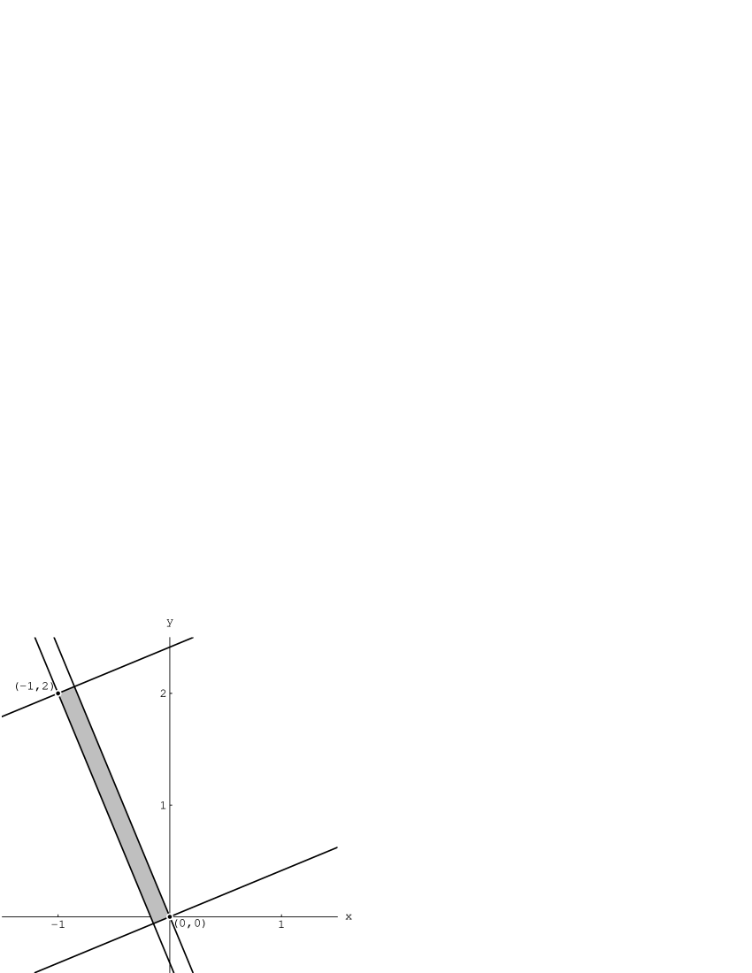
Figure 11. Region containing periodic tails (Example 10.5)

$$\left\{y\in\mathbb{Z}^{2}\biggm{|}-\frac{1}{\left(2+\sqrt{2}\right)^{\frac{3}{2}}}\leq\left\langle y,\psi_{1}\right\rangle\leq 0\text{ and }0\leq\left\langle y,\psi_{2}\right\rangle\leq\frac{3+2\sqrt{2}}{\sqrt{2\left(2+\sqrt{2}\right)}}\right\}$$

$$\qquad=\left\{\begin{pmatrix}x\\ y\end{pmatrix}\in\mathbb{Z}^{2}\Biggm{|}\begin{aligned} \vphantom{\ }&1-\sqrt{2}\leq\left(\sqrt{2}+1\right)x+y\leq 0\\ \vphantom{\ }&\text{and }0\leq-x+\left(\sqrt{2}+1\right)y\leq 3+2\sqrt{2}\end{aligned}\right\}$$

$$\qquad=\left\{\begin{pmatrix}0\\ 0\end{pmatrix},\begin{pmatrix}-1\\ 2\end{pmatrix}\right\}\text{.}$$

See Figure 11. But $R\left(\begin{smallmatrix}0\\ 0\end{smallmatrix}\right)=\left(\begin{smallmatrix}0\\ 0\end{smallmatrix}\right)$ and $R\left(\begin{smallmatrix}-1\\ 2\end{smallmatrix}\right)=\left(\begin{smallmatrix}-1\\ 2\end{smallmatrix}\right)$, thus this gives rise to two cycles with one atom each. Conclusion: the representation associated with (10.19) and (10.21) has two cycles with one atom each, infinitely many cycles with infinitely many atoms each, and no more cycles.

11. Concluding remarks

When finishing this paper, we became aware of the independent paper [DaPi] with some overlapping results. Recall that the Toeplitz algebra $\mathcal{T}_{N}$, for $N<\infty$, has $\mathcal{O}_{N}$ as a quotient. We give a brief discussion of this below. For background references on $\mathcal{T}_{N}$, $\mathcal{O}_{N}$, and the corresponding representations, we use [BEGJ].

The paper [DaPi] describes representations of $\mathcal{O}_{N}$ which are called atomic representations (see next paragraph), and are more general than our permutative ones: they include those of Remark 2.9 and are explained as central extensions (see, e.g., [JoWe]). As a result they get a general decomposition theory for $\mathcal{O}_{N}$ but not for $\mathop{\rm UHF}\nolimits_{N}$. Specifically, the results Theorem 6.4 and Proposition 6.10 in [DaPi] show that, when the restricting assumptions “regular” or “multiplicity-free” in our Theorem 2.7 are removed, then the resulting orthogonal representation decompositions get slightly more refined: there can be continuous parts, or extra representations arising from central extensions; these latter results are in turn closely related to [Jor96] and [Rue88].

Atomic representations of the Cuntz algebra $\mathcal{O}_{N}$ (or rather the Toeplitz algebra $\mathcal{T}_{N}$) are representations such that there exists an orthonormal basis $\left\{e_{n}\right\}_{n=1}^{\infty}$ for the Hilbert space, maps $\sigma_{k}:\mathbb{N}\rightarrow\mathbb{N}$ satisfying (2.4a) and (2.4b) and scalars $\lambda_{i,k}\in\mathbb{T}$ such that

(11.1) $$S_{i}e_{k}=\lambda_{i,k}e_{\sigma_{i}\left(k\right)}$$

(compare (2.2)). In [DaPi], a complete classification up to unitary equivalence of irreducible representations of this kind is given. Except for the left regular representation of the free semigroup with $N$ generators, which corresponds to the unique faithful irreducible representation of $\mathcal{T}_{N}$ (see, e.g., [BEGJ]), all of these are representations of $\mathcal{O}_{N}$. In [DaPi], the representations are described in a different language than ours, but translated to our setting, the classification is as follows: for each $x\in\Omega=\mathop{\mathchoice{\raise 0.0pt\hbox{\raise 1.24167pt\hbox{\lower 8.69167pt\hbox{\Huge$\times$}}}}{\raise 0.0pt\hbox{\raise 0.86417pt\hbox{\lower 6.04916pt\hbox{\huge$\times$}}}}{\raise 0.0pt\hbox{\raise 0.72pt\hbox{\lower 5.04pt\hbox{\LARGE$\times$}}}}{\raise 0.0pt\hbox{\raise 0.59999pt\hbox{\lower 4.2pt\hbox{\Large$\times$}}}}}_{k=1}^{\infty}\mathbb{Z}_{N}$, and each $\lambda\in\mathbb{T}$, define a representation on $\ell^{2}\left(x^{\sim}\right)$ by $S_{k}\delta_{y}=\lambda\delta_{ky}$ (see Section 7). This defines an irreducible representation and, if $x^{\prime}\in\Omega$ and $\lambda^{\prime}\in\mathbb{T}$, the corresponding representations are unitarily equivalent if and only if (i) and (ii) below hold:

1. $x^{\prime}\sim x$ (i.e., $x^{\prime}$, $x$ have the same tail up to translation).

2. If $\mathop{\rm Per}\left(x\right)=m<+\infty$, then $\lambda^{m}={\lambda^{\prime}}^{m}$.

All atomic irreducible representations are of this form, and if $R$ has a finite minimal cyclic orbit $n_{1},n_{2},\dots,n_{m},n_{m+1}=n_{1}$, and $j_{1},j_{2},\dots,j_{m},j_{m+1}=j_{1}$ is the corresponding coding sequence then $\lambda$ can be taken to be any of the $m$ roots of

$$\lambda^{m}=\lambda_{i_{1},n_{1}}\lambda_{i_{2},n_{2}}\cdots\lambda_{i_{m},n_{m}}\text{.}$$

See [DaPi, Theorem 6.4].

In our setting of multiplicity-free function systems, we obtained a discrete decomposition of any permutative representation into mutually disjoint irreducible representations in Theorem 2.7. In the more general case of atomic representations, there are some subrepresentations with a continuous decomposition too. Without describing these in detail (see [DaPi, Proposition 6.10]), a partial explanation of this phenomenon is as follows: the decomposition is over the parameter $\lambda$ considered above, but since the coding map is defined in terms of the maps $\sigma_{i}$ alone, our condition of injectivity of the coding map prevents two different subrepresentations with the same $\sigma_{i}$’s (but different $\lambda$’s) from occurring. It should however be noted that in the extension of Theorem 2.7 to general (not necessarily multiplicity-free) branching function systems, one must consider atomic representations with nontrivial $\lambda$’s in the continuous part of the decomposition of a permutative representation.

The present proof of Theorem 2.7 extends with obvious modifications to the context of atomic representations with injective coding maps, giving a discrete decomposition into the irreducible representations described above, with only one $\lambda$ for each $\sigma_{i}$-class.

Note that, if $x\in\Omega$ is asymptotically periodic with period $m$, $I$ is a string of length $m$ from the tail of $x$, and $\lambda\in\mathbb{T}$, then the irreducible representation described above comes from the sub-Cuntz state determined by

$$\xi=\lambda^{-m}S_{I}\xi\text{;}$$

see Proposition 5.1.

Although the overlap of [DaPi] and the present paper has been emphasized above, the two papers are in other respects rather different. The Gelfand pair aspect of the pair $\left(\mathcal{O}_{N},\mathop{\rm UHF}\nolimits_{N}\right)$ is only treated here, as well as the connection to fractal properties of the dynamical systems coming from the $\bmod{\,\mathbf{N}}$ situation.

As a final comment, we introduce operators that intertwine the two pictures. In [DaPi] the following class of representations of $\mathcal{O}_{N}$ is considered: for $x=\left(j_{1},j_{2},\dots\right)\in\Omega$ fixed, define $x_{m}$ as the word $\left(j_{1},\dots,j_{m}\right)$ and define $\mathcal{F}_{n}x^{-1}$ as the (finite) words in the free group generated by the $N$ symbols in $\mathbb{Z}_{N}$ of the form $ux_{m}^{-1}$ for some $u\in\mathcal{F}_{m}$, where $\mathcal{F}_{m}$ is the free semigroup generated by the $N$ symbols. If $\xi_{v}$, $v\in\mathcal{F}_{n}x^{-1}$ is an orthonormal basis, the representation is defined by

$$S_{i}\xi_{v}=\xi_{iv}\text{.}$$

Now, note that the operation

$$ux_{m}^{-1}\rightarrow ux_{m}^{-1}x$$

defines an isometric intertwiner between this representation and our representation defined in Section 6 by the set of $y\in\Omega$ having the same tail as $x$ up to translation. When $x$ does not have a periodic tail, this intertwiner is a unitary operator, establishing a unitary equivalence between the irreducible representations. If, however, $x$ does have a periodic tail, the intertwiner is merely an $\infty-1$ isometry, and hence the corresponding [DaPi]-representation is an infinite multiple of our irreducible representation, as is also proved in [DaPi, Proposition 6.10(ii)].

It is interesting to note a connection to the construction of unitaries $W$ on a Hilbert space tensor product $\mathcal{H}\otimes\mathcal{H}$ subject to the pentagonal identity

(11.2) $$W_{23}W_{12}=W_{12}W_{13}W_{23}\text{\quad on\quad}\mathcal{H}\otimes\mathcal{H}\otimes\mathcal{H}$$

in the theory of quantum groups (recall the subscripts refer to the usual leg-notation for tensors, that is, $W_{12}=W\otimes\hbox{\small 1\kern-3.3pt\normalsize 1}_{\mathcal{H}}$, $W_{23}=\hbox{\small 1\kern-3.3pt\normalsize 1}_{\mathcal{H}}\otimes W$, and $W_{13}$ acts on the tensor product of the first and last tensor factor of $\mathcal{H}\otimes\mathcal{H}\otimes\mathcal{H}$). Recently Saad Baaj and Georges Skandalis have used a method that is similar to ours in the starting point in their construction of such unitaries $W$ on $\mathcal{H}\otimes\mathcal{H}$ which permute the elements in a tensor product basis. Very recently they have also considered the modification to the effect that the action of $W$ on those basis vectors gets modified with a cocycle factor à la (11.1). We are indebted to S.L. Woronowicz for this information: see [Wor] and [Cun93] for more on the pentagonal identity (11.2).

Acknowledgements

Both the statement and the proof of Proposition 10.1 are entirely due to David Handelman, and likewise the statement and proof of Lemma 3.4 are due to Helge Tverberg. We are indebted to these two colleagues both for permission to publish these results here, and for other useful remarks. This paper was started when P.E.T.J. visited Oslo November 1995 with support from NFR, and continued in Oberwolfach January 1996 where O.B. was supported by NFR. We would like to thank Brian Treadway for an excellent typesetting job, helpful suggestions, and for producing Mathematica-generated graphics to perfection. P.E.T.J. also had helpful discussions with C. Bandt, P. Muhly, R. Curto, R. Strichartz, S. Pedersen, and Yang Wang. P.E.T.J. was also supported by the NSF and a University of Iowa fellowship.

Note on the graphics

The figures of the various reptiles $\mathbf{T}$ in this paper were executed by Brian Treadway using Mathematica and the formulas (3.11) and (3.12) in the form

$$\mathbf{T}=\bigcup_{d\in D}\mathbf{N}^{-1}\left(d+\mathbf{T}\right)\text{.}$$

There is of course a lower limit to the size of the objects drawn, so the series in (3.12) is truncated in the figures. The question of what graphic object to put at the position of each point in the set given by (3.12) with a finite upper limit on $i$ is slightly subtle. The best choice for the reptiles illustrated in this paper seems to be a parallelogram (a square in the case of the Fractal Red Cross, Figure 9.10) that is of the right shape and just large enough to touch the neighboring parallelograms in the picture without overlapping. Compared with the use of a circular dot, this choice enhances the appearance that $\mathbf{T}$ is “compact with non-empty interior”, avoids “aliasing” on the scale of the laser-printer resolution, and makes the graphic easier to rescale without changing its appearance. In this paper, Cloud Three (Figure 7) is drawn with circular dots, but all the other fractal figures are drawn with parallelograms.

References

- [And] George E. Andrews, Number theory, 2nd ed., Dover, New York, 1994 (1st ed., W.B. Saunders Co., Philadelphia–London–Toronto, 1971).
- [Arv] W.B. Arveson, Continuous analogues of Fock space I, Mem. Amer. Math. Soc. 80 (1989), no. 409.
- [Ban91] Christoph Bandt, Self-similar sets V: Integer matrices and fractal tilings of , Proc. Amer. Math. Soc. 112 (1991), 549–562.
- [Ban96] by same author, Self-similar tilings and patterns described by mappings, Proceedings of NATO Advanced Study Institute: Mathematics of aperiodic order (R. Moody and J. Patera, eds.), Kluwer, to appear.
- [BaGe] Christoph Bandt and Götz Gelbrich, Classification of self-affine lattice tilings, J. London Math. Soc. (2) 50 (1994), 581–593.
- [BJR] Chal Benson, Joe Jenkins, and Gail Ratcliff, On Gelfand pairs associated with solvable Lie groups, Trans. Amer. Math. Soc. 321 (1990), 85–116.
- [BeRa] Chal Benson and Gail Ratcliff, A classification of multiplicity free actions, preprint, University of Missouri, 1995.
- [BlDy] P.M. Bleher and F.J. Dyson, The variance of the error function in the shifted circle problem is a wild function of the shift, Comm. Math. Phys. 160 (1994), 493–505.
- [BoCo] J.-B. Bost and A. Connes, Hecke algebras, type III factors and phase transitions with spontaneous symmetry breaking in number theory, Selecta Math. (N.S.) 1 (1995), 411–457.
- [BEEK] Ola Bratteli, G.A. Elliott, D.E. Evans, and A. Kishimoto, Quasi-product actions of a compact abelian group on a -algebra, Tohoku Math. J. 41 (1989), 133–161.
- [BEGJ] Ola Bratteli, David E. Evans, Frederick M. Goodman, and Palle E.T. Jorgensen, A dichotomy for derivations on , Publ. Res. Inst. Math. Sci. (Kyoto University) 22 (1986), 103–117.
- [BraJo] Ola Bratteli and Palle E.T. Jorgensen, Endomorphisms of , II: Finitely correlated states, preprint, The University of Iowa, 1995.
- [BJP] Ola Bratteli, Palle E.T. Jorgensen, and Geoffrey L. Price, Endomorphisms of , Quantization, nonlinear partial differential equations, and operator algebra (William Arveson, Thomas Branson, and Irving Segal, eds.), Proc. Sympos. Pure Math., vol. 59, Amer. Math. Soc., 1996, pp. 93–138.
- [BraRo] Ola Bratteli and Derek W. Robinson, Operator algebras and quantum statistical mechanics, 2nd ed., vol. I, Springer-Verlag, Berlin–New York, 1987.
- [BreJo] Berndt Brenken and Palle E. T. Jorgensen, A family of dilation crossed product algebras, J. Operator Theory 25 (1991), 299–308.
- [BLSTW] John Brillhart, D. H. Lehmer, J. L. Selfridge, Bryant Tuckerman, and S. S. Wagstaff, Jr., Factorizations of , 2nd ed., Contemp. Math., vol. 22, Amer. Math. Soc., Providence, RI, 1988.
- [CoRy] Albert Cohen and Robert D. Ryan, Wavelets and multiscale signal processing, Chapman & Hall, London–New York, 1992, 1995, in English translation.
- [Cun77] Joachim Cuntz, Simple -algebras generated by isometries, Comm. Math. Phys. 57 (1977), 173–185.
- [Cun93] by same author, Regular actions of Hopf algebras on the -algebra generated by a Hilbert space, Operator algebras, mathematical physics, and low-dimensional topology (Istanbul, 1991) (Richard Herman and Betul Tanbay, eds.), Res. Notes Math., vol. 5, A K Peters, Wellesley, MA, 1993, pp. 87–100.
- [DDL] Stephan Dahlke, Wolfgang Dahmen, and Vera Latour, Smooth refinable functions and wavelets obtained by convolution products, Appl. Comput. Harmon. Anal. 2 (1995), 68–84.
- [DaLa] X. Dai and D. Larson, Wandering vectors for unitary systems, and orthogonal wavelets, to appear in Mem. Amer. Math. Soc.; preprint, Texas A. & M. University, 1995.
- [Dau] Ingrid Daubechies, Ten lectures on wavelets, CBMS-NSF Regional Conf. Ser. in Appl. Math., vol. 61, Soc. for Industrial and Applied Math., Philadelphia, 1992.
- [DaPi] K.R. Davidson and D.R. Pitts, Free semigroup algebras, preprint, University of Nebraska, University of Waterloo, 1996.
- [EHK] Stanley Eigen, Arshag Hajian, and Shizuo Kakutani, Complementing sets of integers—a result from ergodic theory, Japan. J. Math. (N.S.) 18 (1992), 205–211.
- [EvKa] David E. Evans and Yasuyuki Kawahigashi, Quantum symmetries on operator algebras, monograph series, Oxford University Press, to appear.
- [Fur] H. Furstenberg, Recurrence in ergodic theory and combinatorial number theory, Princeton University Press, 1981.
- [Gel] Götz Gelbrich, Self-affine lattice reptiles with two pieces in , Math. Nachr. 178 (1996), 129–134.
- [Gil] William J. Gilbert, The division algorithm in complex bases, Canad. Math. Bull. 39 (1996), 47–54.
- [GHJ] Frederick M. Goodman, Pierre de la Harpe, and Vaughan F.R. Jones, Coxeter graphs and towers of algebras, Springer-Verlag, New York, 1989.
- [GrMa] K. Gröchenig and W. R. Madych, Multiresolution analysis, Haar bases, and self-similar tilings of , IEEE Trans. Inform. Theory 38 (1992), 556–568.
- [Haa] Uffe Haagerup, Orthogonal maximal abelian -subalgebras of the matrices and cyclic ’th roots, preprint, Odense University, 1995.
- [Han] David Handelman, Spectral radii of primitive integral companion matrices and log concave polynomials, Symbolic dynamics and its applications (New Haven, CT, 1991) (Peter Walters, ed.), Contemp. Math., vol. 135, Amer. Math. Soc., Providence, RI, 1992, pp. 231–237.
- [HRW] Peter N. Heller, Howard L. Resnikoff, and Raymond O. Wells, Jr., Wavelet matrices and the representation of discrete functions, Wavelets: A tutorial in theory and applications (Charles K. Chui, ed.), Wavelet Anal. Appl., vol. 2, Academic Press, Boston–San Diego, 1992, pp. 15–50.
- [Ho] Mark C. Ho, Properties of slant Toeplitz operators, preprint, Purdue University, 1996.
- [Hou] Christian Houdré, Wavelets, probability, and statistics: some bridges, Wavelets: Mathematics and applications (J.J. Benedetto et al., eds.), CRC, Boca Raton–Ann Arbor, 1994, pp. 365–398,.
- [Jor95] Palle E.T. Jorgensen, Harmonic analysis of fractal processes via -algebras, preprint, The University of Iowa, 1995.
- [Jor96] by same author, A duality for endomorphisms of von Neumann algebras, J. Math. Phys. 37 (1996), 1521–1538.
- [JoPe92] Palle E. T. Jorgensen and Steen Pedersen, Spectral theory for Borel sets in of finite measure, J. Funct. Anal. 107 (1992), 72–104.
- [JoPe94] by same author, Harmonic analysis and fractal limit-measures induced by representations of a certain -algebra, J. Funct. Anal. 125 (1994), 90–110.
- [JoPe95] by same author, Estimates on the spectrum of fractals arising from affine iterations, Fractal geometry and stochastics (Christoph Bandt, Siegfried Graf, and Martina Zähle, eds.), Progress in Probability, vol. 37, Birkhäuser, Basel, 1995, pp. 191–219.
- [JoPe96] by same author, Harmonic analysis of fractal measures, Constr. Approx. (1996).
- [JoWe] Palle E.T. Jorgensen and R.F. Werner, Coherent states of the -canonical commutation relations, Comm. Math. Phys. 164 (1994), 455–471.
- [KMW] Y. Katayama, K. Matsumoto, and Y. Watatani, Simple -algebras arising from -expansions of real numbers, preprint, 1996.
- [Ken] Richard Kenyon, Self-replicating tilings, Symbolic dynamics and its applications (New Haven, CT, 1991) (Peter Walters, ed.), Contemp. Math., vol. 135, Amer. Math. Soc., Providence, RI, 1992, pp. 239–263.
- [Knu] Donald E. Knuth, The art of computer programming: Vol. 2: Seminumerical algorithms, 2nd ed., Addison-Wesley Publishing Co., Reading, Mass., 1981 (1st ed. 1969).
- [Lac] M. Laca, Endomorphisms of and Cuntz algebras, J. Operator Theory 30 (1993), 85–108.
- [Lag85] Jeffrey C. Lagarias, The problem and its generalizations, Amer. Math. Monthly 92 (1985), 3–23.
- [LaWa1] Jeffrey C. Lagarias and Yang Wang, Haar bases for and algebraic number theory, J. Number Theory 57 (1996), 181–197.
- [LaWa2] by same author, Nonnegative radix representations for the orthant , Trans. Amer. Math. Soc. 348 (1996), 99–117.
- [LeV] William J. LeVeque, Fundamentals of number theory, 2nd ed., Dover, New York, 1996 (1st ed., Addison-Wesley, Reading, Mass., 1977).
- [LiMa] Douglas Lind and Brian Marcus, An introduction to symbolic dynamics and coding, Cambridge University Press, 1995.
- [Mau] R. Daniel Mauldin, Infinite iterated function systems: Theory and applications, Fractal geometry and stochastics (Christoph Bandt, Siegfried Graf, and Martina Zähle, eds.), Progress in Probability, vol. 37, Birkhäuser, Basel, 1995, pp. 91–110.
- [Odl] A.M. Odlyzko, Nonnegative digit sets in positional number systems, Proc. London Math. Soc. (3) 37 (1978), 213–229.
- [PaTa] Jacob Palis and Floris Takens, Hyperbolicity and sensitive chaotic dynamics at homoclinic bifurcations, Cambridge Studies in Advanced Mathematics, vol. 35, Cambridge University Press, 1993.
- [Pow88] Robert T. Powers, An index theory for semigroups of -endomorphisms of and type factors, Canad. J. Math. 40 (1988), 86–114.
- [PoPr] Robert T. Powers and Geoffrey L. Price, Cocycle conjugacy classes of shifts on the hyperfinite factor, J. Funct. Anal. 121 (1994), 275–295.
- [PoSt] Robert T. Powers and Erling Størmer, Free states of the canonical anti-commutation relations, Comm. Math. Phys. 16 (1970), 1–33.
- [Pri] Geoffrey L. Price, Shifts on type factors, Canad. J. Math. 39 (1987), 492–511.
- [Rib] Paulo Ribenboim, The book of prime number records, 2nd ed., Springer-Verlag, New York–Berlin, 1989.
- [Rud88] Daniel J. Rudolph, Rectangular tilings of and free -actions, Dynamical systems (College Park, MD, 1986–87), Lecture Notes in Math., vol. 1342, Springer, Berlin–New York, 1988, pp. 653–688.
- [Rud89] by same author, Markov tilings of and representations of actions, Measure and measurable dynamics (Rochester, NY, 1987), Contemp. Math., vol. 94, Amer. Math. Soc., Providence, RI, 1989, pp. 271–290.
- [Rue88] David Ruelle, Noncommutative algebras for hyperbolic diffeomorphisms, Invent. Math. 93 (1988), 1–13.
- [Rue94] by same author, Dynamical zeta functions for piecewise monotone maps of the interval, CRM Monograph Series, vol. 4, Amer. Math. Soc., Providence, RI, 1994.
- [Sen] Marjorie Senechal, Quasicrystals and geometry, Cambridge University Press, 1995.
- [Str94] Robert S. Strichartz, Self-similarity in harmonic analysis, J. Fourier Anal. Appl. 1 (1994), 1–37.
- [Str95] by same author, Fractals in the large, preprint, Cornell University, 1995.
- [Wor] S. L. Woronowicz, From multiplicative unitaries to quantum groups, Internat. J. Math. 7 (1996), 127–149.