Vladimir Matveev111vmatveev@physik.uni-bremen.de,
Peter Topalov222topalov@banmatpc.math.acad.bg
Abstract
We show that an invariant surface allows to construct the Jacobi vector
field along a geodesic and construct
the formula for the normal
component of the Jacobi field. If a geodesic
is the transversal
intersection of two invariant surfaces (such situation we have,
for example, if the geodesic is hyperbolic),
then we can construct
a fundamental solution of the the Jacobi-Hill equation .
This is done for quadratically integrable geodesic flows.
§1. Introduction.
1.1. Definitions.
Suppose is a Riemanian metric on a surface ,
a curve
is a geodesic.
We will assume that the parameter of the geodesic
is natural or natural, multiplied by a constant.
Definition 1
Geodesic variation of a geodesic
is called the smooth
mapping such that
1)
for any fixed
the curve (as the curve of parameter
) is a geodesic,
2)
for any .
Definition 2
Jacobi vector field
along the geodesic is
the vector field
, where
is a geodesic
variation of the geodesic .
By definition, Jacobi vector field is a smooth vector field along the
geodesic.
Definition 3
Jacobi vector field is called
normal if it is orthogonal
to the geodesic at every point of the geodesic.
It is known that the projection of a Jacobi field to the vector field of
normals to the geodesic is a normal Jacobi vector field.
The length of a normal Jacobi vector field satisfies
the Jacobi-Hills equation
for the normal component ,
where is the Gauss curvature
and is the natural parameter (see, for example,
[1] or [2]).
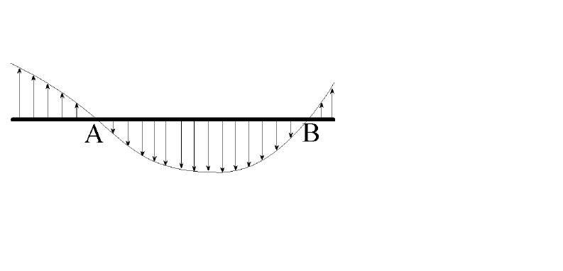
Consider real numbers . Denote by the point
, denote by the point
.
Definition 4
The points and are called conjuate
along the geodesic
if there exists a non-zero Jacobi vector field along
the geodesic
such that . (Figure 1)
Figure 1:
The point can coincide with the point
. It happens if the geodesic is closed
or self-intersecting. In the first case the point is called self-conjugate along the
geodesic .
1.2. Jacobi vector fields as the projection of invariant
vector fields from the co-tangent space.
The metric allows to identify canonically the tangent
and co-tangent bundles of the
surface
. Therefore we have a scalar product and a norm on every
co-tangent plane. For example,
suppose
in coordinates
reads . Then the scalar product on
is given by the formula
.
Definition 5
Geodesic flow of the metric is called the Hamiltonian system
on with
the Hamiltonian , where is momentum and
is the norm.
In particular, the Hamiltonian of the geodesic flow of the metric
is given by the formula
.
It is known that the trajectories of the geodesic
flow projects onto the geodesics.
Definition 6
An imbeded into surface
is called invariant
if the vector field of the geodesic flow is tangent to .
Definition 7
Let be the solution of the geodesic flow.
The vector field along the curve is called invariant
if
it is invariant with respect to the the geodesic flow.
In other words, consider the one parametric family
of mappings . The mapping
moves a point
along the trajectory of the geodesic flow
during the time .
The vector field is called invariant
if for any the differential
takes the vector field to itself.
In §2 we will show that a
geodesic variation allows to canonically construct
an invariant surface;
a Jacobi vector field allows to canonically construct
an invariant vector field;
the projection of the
invariant vector field is the Jacobi vector field and
the composition of the projection and an
imbedding of the invarant surface is the geodesic variation.
1.3. Jacobi vector fields of integrable geodesic flows.
A geodesic flow is
called integrable if it
is integrable as a Hamiltonian system.
That is there exists a smooth function
such that
1)
is constant on the trajectories of the geodesic flow
2)
the differentials and are linear independent
almost everywhere.
The function is called an integral.
Note that the geodesic flow preserves the vector field
.
Since that, the projection of the vector field
is a Jacobi vector field.
Using this, we can construct a number of pairs of conjugate points.
Let be a Louville torus of an integrable geodesic flow.
Restrict the natural projection to the torus .
A connected component of the set of
critical points of is called
a caustic. It is known ( see, for example, [3])
that a caustic
is a smooth simple curve and can not intersect other caustic.
RemarkSometimes caustics are called
the projection of the set of
critical points of the mapping
.
According to our definition,
caustics are curves in the
fase space .
Suppose the intersection of the trajectory
with the caustics includes
points
and .
We prove that the projections
and
are conjugate along the
geodesic . Indeed,
consider the restriction of
the vector field
to the Liouville
torus . Consider
the projection
.
Since the rank of
the projection
is less than 2 in the points
and , we see that
the projections of the vector fields
and
are parallel in the points.
Therefore the normal component of the vector field
equals zero in the points and . Thus points
and are conjugte.
1.4. Jacobi vector fields for a hyperbolic geodesic.
Definition 8
A closed geodesic is
called em hyperbolic if
the corresponding trajectory of
the geodesic flow is hyperbolic.
That is if we restrict the geodesic flow to the
isoenergy surface (we denote isoenergy surface by )
then the multipliers
of
the trajectory not lie
on the
unit circle.
It is known that
in a regular neighborhood of a
hyperbolic trajectory there exists
a pair of invariant two-dimensional surfaces
( and ). The intersection of the
surfaces coincides with
(See, for example, [4]).
An invariant surface allows to construct
a solution of the Jacobi-Hill equation.
In §3 we will show that the
solutions that correspond to the surfaces and
are
not proportional.
Therefore we have a fundamental solution
of the Jacobi-Hill equation .
Assume that the geodesic flow is integrable, and the integral is a Bott function.
That is the restriction of the integral to the isoenergy
surface satisfies the following properties (we denote the restriction by ):
1.
The critical manifolds of are compact sets.
2.
If is an arbitrary
2-disk that is transversal with critical manifolds,
then the restriction
is a Morse function.
Suppose a connected component of the set of
critical points is homeomorphic to
the circle. Consider a transversal disk.
The
dimension of the transversal disk
equals 2. The restriction of the function
to the transversal disk
has Morse singularity of index 0,2, or 1.
In the last case the connected component
of the critical set is called a saddle circle.
Hyperbolic trajectories of a Bott integrable geodesic flow
are saddle circles.
Remark Let a trajectory of a
Bott integrable
Hamiltonian system be
a hyperbolic trajectory.
Then it is a saddle circle.
The reverse statement is not true.
There exist saddle circles that are
not hyperbolic trajectories.
Consider the Liouville fiber that contains a saddle circle.
In a neighborhood of a point of the saddle circle the Liouville fiber is
homeomorphic to a pair of intersecting surfaces.
Recall that a saddle circle is called
nonorientable if the intersection
of the Liouille
fiber with a regular neigborhood of the saddle circle
is homeomorphic to the self-intersecting
Möbius band.
A saddle circle is called orientable
the intersection of the Liouville fiber with a saddle neighborhood
is homeomorphic to two intersecting annuli.
Consider a closed geodesic .
Let a point be self-conjugate
along the geodesic. Consider the set of points
conjugate to .
Denote by the number of elements in the set.
It is known that does not depend on the
choice of the initial point .
If for the point there are no conjugate points
along , then
by defintion put .
Theorem 1
Suppose is an orientable surface,
the geodesic flow of a metric
is integrable, and is a saddle circle.
Then
•
if the circle is nonorientable, then
is odd number,
•
if the circle is orientable,
then
is even nuber.
The statement of the result for nonorientable saddle circles
were proved by
A. Wittek.
Proof. Let a saddle circle be orientable.
Consider the Liouville fiber that contains .
By definition, a regular
neighborhood of the Liouville fiber
is homeomorphic to a pair of intersecting annuli.
Denote by oe of the annuli.
Consider a
vector field that is invariant and that is tangent
to
.
Denote by the projection of the vector field
.
Using the theorem of the existence and
uniqueness
of the solution of a differential equation, we have
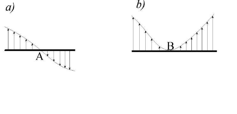
that in a
neighborhood of a zero point a normal Jacobi vector
field behaves as it is shown on
Diagramm 2(a) (the situation of Diagramm 2(b) is forbidden).
That is, the frame (velocity vector of the geodesic,
Jacobi vector field)
has different orientation at different sides of the
geodesic .
Figure 2:
Since has no zero points, we see that the frame
(the velocity vector of , )
has the same orientation with respect
to the invariant surface in every point of the geodesic.
Hence the vector field has the same direction after and before
the circuit along the geodesic. Hence, the number
of zeros of is an even number.
Proved.
1.6. Jacobi vector fields along hyperbolic geodesics
of quadratically integrable geodesic flows.
Definition 9
A geodesic flow is called linear integrable if it admits an integral
such that in a neighborhood of any point the integral
is given by the formula
, where are coordinates
on the surface,
are the corresponding momenta,
and are smooth functions of two variables.
Definition 10
A geodesic flow is called
quadratically integrable,
if it is not linear integrable and if
it admits an integral such that in a neighborhood of any
point the integral is given by the formula
, where
are smooth
functions of two variables.
Quadratically and linear integrable geodesic flows on closed surfaces
are comletely described. In [6] V.V. Kozlov proved that there are no
linear and quadratic integrable geodesic flows on the surfaces of genus .
Linear and quadratically integrable geodesic flows on the sphere
were described by V.N. Kolokolzov in [8].
Quadratically integrable geodesic flows on the torus were described
by I.K. Babenko and N.N. Nekhoroshev in [10] (see, also, [13]).
In §5 we describe hyperbolic trajectories
and invariant surfaces of
quadratically inegrable geodesic flows and obtain
fundamental solutions of the Jacobi-Hill equation
along hyperbolic geodesics.
§2. Canonical frame on .
Commutative relations for it.
Let be a Riemannian metric on the oriented surface .
Consider the tangent bundle .
The space of non-zero vectors of
is denoted by .
The aim of this section is to canonically construct
a frame (the vectors of the
frame will be denoted by ) in
every point of
. Since the metric allows to identify the
tangent and co-tangent
bundles of the surface , we will
have the canonic frame in every point of .
2.1. The frame. Let be an arbitrary point
of the surface ,
let be a tangent vector at the point .
The vector is a point of .
Denote by the vector at the point
such that
, the angle between and is equal to , and
the frame is positive. In other words,
rotates a vector by the angle .
Consider the vector
at the point .
Denote by the vector field .
By definition, put
Consider the so-called ”Liouville vector field” ([2]).
Recall, that the vector field is defined in the following way.
Consider the one-parameter group of self-diffeomorphisms .
. Put by definition
.
Direct calculations show that for the
vectors are linear independent.
Therefore the quadruple is a frame.
2.2. Commutative relations for the vectors of the frame.
Denote by the function . The function
is a smooth function on
.
Lemma 1
where , is the Gaussian
curvature of the metric
on the surface .
The first three relations follows from [7].
The last three relations were proved in [2].
Consider a geodesic trajectory . Consider an invariant
vector field
along . Let
Since the vector field is invariant, we have .
Using lemma 1, we obtain the following system:
(1)
If the length of the vector equals 1, then from
the first two equations it follows Jacobi-Hills
equation .
Note, that in this case
is normal component
of the vector field .
Projection of the vector field is the horizontal component
of the vector field . Hence the projection of the vector field
is equal to , where
is the normal vector (to the geodesic) of length 1.
We shall prove that for every Jacobi vector field there exists
an invariant vector field such that .
Consider a Jacobi vector field along the geodesic .
Denote by
the normal component of the vector field , denote by
the horizontal component of the vector field .
By definition, , where
is a geodesic variation of the geodesic
. Consider
the vector field along the
trajectory .
Evidently the vector field is invariant. Indeed,
.
Moreover, we see that the vector field
equals
where , are smooth functions,
is the normal component of the Jacobi vector field , and
is the horizontal component of
the Jacobi vector field .
§3. Fundamental solution of the
Jacobi-Hill equation
for hyperbolic geodesics.
Consider a geodesic trajectory .
Denote by the geodesic .
Suppose we have an 1-dimension subspace in every tangent
space at the points of the
geodesic trajectory.
Suppose the set of the subspaces
is invariant with respect ot the geodesic
flow.
Consider the projection of every subspace along the plane
to the plane . Denote the projection by
.
Consider the mapping . Then
is 1-dimensional
subspase in the tangent planes at
the points of the geodesic. Using Lemma 1, we see that
the set of is invariant with respect to
the geodesic flow.
Since the vector projects to , and since
the projection of
is orthogonal to the geodesic , we have that
is orthogonal to the geodesic .
Consider a direction vector field
of the set .
Let an invariant vector field be parallel to .
Then equals ,
where is
a smooth function.
Suppose the coordinates of the vector field
in the frame are equal to
.
(Since lies in the plane , we see that
the second and the fourth coordinates must be equal to .)
is invariant with respect to the geodesic flow, and the projection
of it is a Jacobi vector field.
In particular, the function
(3)
satisfies the Jacobi-Hill equation
.
Suppose a geodesic
is hyperbolic. Then we have
two invariant intersecting surfaces in a regular neighborhood of .
Consider the subspaces that are tangent to these surfaces.
Since the intersecting surfaces are
invariant then the tangent subspaces
are invariant, too. Then the projection of the surfaces to the planes
along the planes
is two families of invariant 1-dimension subspace.
Arguing as above, we can construct
two Jacobi vector fields. The Jacobi vector field are nonproportional.
Hence they define a fundamental solution of the Jacobi-Hill equation.
Remark It is easy to find the coordinates .
Let the metric has the form
. Let a field equals
. The coefficients
are functions of . Then,
(4)
(5)
Remark Now let the projection of an invariant set of subspaces
is not orthogonal to the geodesic.
Consider the projection of every subspace along the plane
to the plane . Denote the projection by
.
Let be a direction vector field of the subspaces , denote by
the
projection of the vector field along the plane
to the plane .
Suppose that in the coordinate system vector fields
, are equal to ,
, respectively. Then,
Now let the curve is a geodesic.
We do not
require the parameter to be natural or natural,
multipling by a constant. Let the cordinates
be isothermal.
That is the metric has the form
. Suppose a geodesic trajectory
projects into the geodesic
. Let be the length of the
velocity vector of the geodesic in the parameter .
Consider the functions as the functions of the
new parameter .
Lemma 2
Let be the connection between the
parameter and the parameter .
Consider the function
Then the function is
a solution of the Jacobi-Hill equation.
The proof is by direct calculation.
§4. Quadratically integrble geodesic flows
on the torus and on the sphere.
4.1. Quadratically integrable geodesic flows on the torus.
Let be a positive number.
Denote by the circle with a smooth parameter .
Definition 11
A metric on the torus is called Liouville
if for an appropriate positive and for appropriate
nonconstant positive functions , there exist
a diffeomorphism that takes the metric
to the metric , where are
parameters on , respectively.
Definition 12
A metric on the torus is called pseudo-liouville
if there exists a Liouville metric on the torus and
a covering such that .
RemarkSince the identity mapping is a 1-sheet covering
a Liouville metric is a pseudo-liouville metric.
The geodesic flow of a metric on the torus is quadratically
integrable iff the metric is pseudo-liouville.
4.2. Quadratically integrable geodesic flows on the sphere.
Consider the torus . Let for smooth functions
,
the following conditions hold
1
The functions , are nonnegative.
The function equals
zero only in the points 0 and
;
The function equals
zero only in the points 0 and
;
2
.
3
For any , and
.
Consider the involution ,
. The fixed points of are:
, ,
and .
Consider the factorspace
.
is homeomorphic to
the sphere. Consider the following structure of a smooth 2-dimensional
manifold on .
Denote by
the dual to the involution
mapping. In other words, the mapping
takes a point
to the point
.
Consider smooth structure on such that the mapping
is a smooth branched covering
with branch points
of the branch
index 1.
Obviously, the smooth structure exists.
Note, that the mapping
in the appropriate coordinates is
the Weierstrass -function with half-periods and
.
Consider the degenerate metric
on the torus
. The form
is positive definite everywhere exept of at the
points
,
,
, and
.
Since the function is preserved by the involution
, we see that the metric
induces a metric on the sphere
without branch points.
The conditions on the functions , allow to complement the
metric in the branch points. Denote by
the complemented metric.
Definition 13
A metric on the sphere is called a Kolokoltzov metric
if for an appropriate positive number and for appropriate
functions , there exists a diffeomorphism
that takes the metric to the metric
.
The geodesic flow of a metric
on the sphere is quadratically integrable
iff the metric is a Kolokoltzov metric.
RemarkIf the functions and are smooth functions,
then the metric
is smooth on without the branch points.
The metric
is -smooth in a branch point iff the following condition holds.
In the branch point Taylor series of the function as the function of
coincides till -member
with Taylor series of the function as the function of (see [9]).
In other words, the metric
is -smooth in a branch point
if for any natural .
4.3. Hyperbolic trajectories of the quadratically integrable
geodesic flows on the torus.
Consider the isoenergy surface
Following the paper [11] we describe the set of critical circles of
the geodesic flow. For simplicity suppose are Morse functions.
Denote by ( ) the set of critical points of the function
(respetively, ).
In [11], E. Selivanova proved that the set of critical points
of the metric is the union of the sets
Besides, the circle
is a saddle
circle iff the point is a nodegenerate critical point of the
Morse index .
It is possible to prove that the saddle circles of quadratically
integrable geodesic
flow on the torus are hyperbolic
trajectories.
4.4. Saddle circles of the quadratically integrable geodesic flow on the
sphere.
Suppose the functions , satisfy the conditions
1,2,3 from section 4.2. Consider the torus
with the (degenerate) metric
Consider the torus without
the points
,
,
,
. Then is a metric.
Using the previous section, we have that the saddle circles of the
metric are the circles
and
The involution rerrange
pairs of circles. Since that, any
pair factorize to a saddle circle. Such saddle circles are called
simple. If the projection of the saddle circle of the geodesic flow
does not contain the point from the set
,
,
,
, then the circle is simple.
There exist two nonsimple saddle
circles
(we denote them by ,
) of the geodesic
flow of a Kolokoltzov metric.
Consider the segments
The segments factorize to the circle ( denoted
by ),
Since the restriction of the integral to the transversal disk to
an intervals has a singularity of Morse
index 1, we see that
is a saddle circle.
Note, that the simple saddle circles of the geodesic flow
of a Kolokoltzov metric are hyperbolic trajectories.
There exist examples of the Kolokoltzov metric such that
the saddle circles
(, ) are not hyperbolic trajectories.
§5. Fundamental solution of the Jacobi equation for the hyperbolic geodesics
of quadratically integrable geodesic flows.
The formulas (3–5) allows to construct a fundamental solution of
the Jacobi-Hill equation for saddle circles of the quadratically
integrable geodesic flows.
5.1. Torus.
Without loss of generality it can be assumed that
a saddle circle as the set of points coincides with the set
, and that
.
Consider the Liouville fiber, which contains the saddle circle.
The Liouville fiber is the set
.
It is easy to see that the vectors
are
1)
tangential to
the Liouville fiber
and
2)
lie in the planes .
Therefore the vectors
are direction vectors
of two families of invariant 1-subspases.
Using Lemma 2, we get the following equations for
, .
(6)
(7)
Combining (6, 7) with the formula for ,
we get a fundamental solution
of the Jacobi-Hill equation:
(8)
Remark Since the function increase and since
the function
decrease, we see that there are no conjugate points
along the hyperbolic geodesics
of a quadratically integrable geodesic flow on the torus.
5.2. Sphere. For a simple geodesic
the answer coinsides with the answer for
the torus.
Consider the nonsimple saddle circle .
The circle can be represented as four glued segments
, , , . Using (8), we see that
the pair of functions
(9)
is a fundamental solution on the segments
.
Arguing as above,
the pair of functions
(10)
is a fundamental solution on the segments , .
We shall glue the fundamental solutions of the Jacobi-Hill eqution
in the points
,
,
.
Consider the point . We have to find constants
,
,
,
such that
Therefore,
(11)
(12)
Arguing as above, we can
glue the fundamential solutions in the points
,
,
,
. We obtain a fundamental solution
of the Jacobi-Hill equation along the geodesic line
.
Consider a point
. Using the Sturm-Liouville theorem, we see that there exists a
point
that is conjugate to the point .
Using (11-12), we get the following equation for :
(13)
References
[1]B.A. Dubrovin, C.P. Novikov, A.T. Fomenko
Modern grometry. Methods and applications.// Nauka:
Moscow. 1979.
English transl. Springer-Verlag:New York Berlin Heidelberg, Grad. Texts Math, 93, 1984.
[2]Besse Manifolds all of whose geodesics are closed.//Springer-Verlag Berlin Heidelberg. 1978
[3]M.L. Bialy, L.V. Poltervich
Lagrangian singularities of invariant tori of Hamiltonian systems with
two degrees of freedom. //Invent. Math. 97, pp.291–303. 1989.
[4] Editor – D.V.
Anosov Smooth dynamic systems// Itogi Nauki i Techniki, sovremennye problemy matematiki. Fundameentalnye napravleniya, vol. 2, 1974.
[5]A.T. Fomenko The topology of the surfaces of the constant energy in integrable Hamiltonian systems and the obstructions to the integrability. // Izv. Akad. Nauk Sintegrals of geodesic flows on compact surfaces.//
. ̵ᮨ SSR 287 No. 5, 1986. English transl.:
Math. USSR, Izv. 29, No. 3, pp 629–659. 1987.
[6]V.V. Kozlov
Topological obstructions for integrability of natural mechanic systems.
//Doklady AN SSSR , 1979. Vol. 249,N6, .1299–1302.
[7]S. Kobayashi, K. Nomizu Foundations of the
Differential Geometry.// Wiley-Interscience, New York, 1969.
[8]V.N. Kolokoltzov Geodesic flows with an additional polynomial in velocities integral on two-dimensional manifolds.// Izv. AN SSSR, ser. matem., 1982. 46, No. 5. pp 994–1010.
[9]V.N. Kolokoltzov Polynomial integreals of geodesic flows on the compact sufaces.// Ph.D. Theses, Moscow State University, 1984.
[10]I.K. Babenko, N.N. Nekhorochev On the complex structures on two-dimensional tori that admit metrics with nontrivial quadratic integral.
// Mat. Zametki, 58, No. 5, pp 643–652. 1995.
[11]E.N. Selivanova Classification of the geodesic flows of the Liouville metrics up to topological equivalence// Mat. Sbornik 183, No. 4, pp
69–86. 1992.
[12]E.N. Selivanova Trajectory isomorphisms of Liouville systems on the two-dimensional torus.// Mat. Sbornik 186, No.10, 1995.
[13]V.S. Matveev Quadratically integrable geodesic flows on the
torus and on the Klein bottle. //Regular and chaotic dynamics. N1. Vol.2. 1997.
[14]V.S. Matveev , P.J. Topalov Conjugate points
of the hyperbolic trajectories of the quadatic integrable geodesic flows.//
Vestn. MGU. Ser. mat., mech. 1997.