Morse theory on the loop space of flat tori and symplectic Floer theory

Abstract.

We use closed geodesics to construct and compute Bott-type Morse homology groups for the energy functional on the loop space of flat $n$-dimensional tori, $n\geq 1$, and Bott-type Floer cohomology groups for their cotangent bundles equipped with the natural symplectic structure. Both objects are isomorpic to the singular homology of the loop space. In an appendix we perturb the equations in order to eliminate degeneracies and to get to a situation with nondegenerate critical points only. The (co)homology groups turn out to be invariant under the perturbation.

1. Introduction

We are going to use the set of critical points of the symplectic action functional

(1) $${\cal A}_{H_{0}}\;:\;\Lambda T^{*}T^{n} \rightarrow {\mathbb{R}}$$

$$z \mapsto \int_{{\mathbb{R}}/{\mathbb{Z}}}z^{*}\Theta-\int_{0}^{1}H_{0}(z{\scriptstyle(}t{\scriptstyle)})\>dt\;,$$

to construct an algebraic chain complex whose homology represents the singular homology of the free loop space of $T^{n}$. In (1) $\Theta$ is the Liouville form on $T^{*}T^{n}$ and the Hamiltonian $H_{0}\>:\>T^{*}T^{n}\rightarrow{\mathbb{R}}$ is given by $z\mapsto\frac{1}{2}|z|^{2}$, where the metric $g$ on $T^{n}\subset{\mathbb{C}}^{n}$ is induced by the real part of the hermitian inner product on ${\mathbb{C}}^{n}$. In our construction of the chain complex we follow the ideas in [RT] and [AB]. Because $H_{0}$ is time independent, the set $Crit\>{\cal A}_{H_{0}}$ of critical points of ${\cal A}_{H_{0}}$ cannot be discrete: Assume a critical point $z$ is a nonconstant loop, then $S^{1}\ni\tau\mapsto z(\cdot+\tau)$ produces a $S^{1}$-family of critical points. Therefore standard nondegenerate Floer theory does not apply. We have to take into account the singular [RT] or de Rham [AB] (co)homology of $Crit\>{\cal A}_{H_{0}}$ leading to a double complex.

In the general case the $L^{2}$-gradient flow lines of ${\cal A}_{H_{0}}$ between different connected components $Crit\>{\cal A}_{H_{0}}$ will enter the construction, but here they cannot exist as different components lie in different connected components of $\Lambda T^{*}T^{n}$. Therefore the Bott-type Floer complex reduces to the singular chain complex of the critical manifolds, whose components are diffeomorphic to $T^{n}$, and so

(2) $$HF^{-i}_{a,Bott}(T^{*}T^{n},H_{0},g;{\mathbb{Z}})=\begin{cases}\bigoplus_{l\in{\mathbb{Z}}^{n},|l|\leq|k|}{\mathbb{Z}}^{\binom{n}{i}}&,-i=-n,\ldots,0\\ 0&,\text{else}\end{cases}$$

where $a=2\pi^{2}|k|^{2}$ indicates that we consider only loops in $T^{*}T^{n}$ whose symplectic action is less or equal to $a$. This set is denoted by $\Lambda^{a}T^{*}T^{n}$. The direct sum in (2) parametrizes the connected components of $\Lambda^{a}T^{*}T^{n}$. The grading $-i$ is provided by a generalized Conley-Zehnder index associated to any element of $Crit\>{\cal A}_{H_{0}}$ plus half the local dimension of $Crit\>{\cal A}_{H_{0}}$.

On the other hand one can perturb $H_{0}$ by a time dependent function (potential) $V$ on $T^{n}$, such that $Crit\>{\cal A}_{H_{0}+V}$ consists of isolated critical points and in this case standard Floer theory applies (this is the approach in [SW] and [W99]). The grading then is given by the standard Conley-Zehnder index [CZ] and the trajectories of the negative gradient flow of ${\cal A}_{H_{0}+V}$ connect critical points of increasing nonpositive indices. That is why the cohomology notation is used.

It is known that the Hamiltonian flow on $T^{*}T^{n}$ generated by $H_{0}$ gives rise to geodesics of $(T^{n},g)$ when projected to the base $T^{n}$. In this way $Crit\>{\cal A}_{H_{0}}$ corresponds precisely to the set of closed geodesics of $(T^{n},g)$, which are the critical points of the classical action functional on the free loop space of $T^{n}$ (called energy functional in Riemannian geometry)

(3) $${\mathcal{I}}_{0}\;:\;\Lambda T^{n} \rightarrow {\mathbb{R}}$$

$$\gamma \mapsto {\scriptstyle\frac{1}{2}}\int_{0}^{1}|\dot{\gamma}(t)|^{2}\>dt\;.$$

As the critical points of the symplectic and the classical action are naturally identified we denote them simply by $Crit$. Observe that on $Crit$ both functionals agree. This continues to hold in the presence of a time-dependent perturbation term. We use closed geodesics $\gamma$ with ${\mathcal{I}}_{0}(\gamma)\leq a$ to construct Bott-type Morse chain groups graded by the Morse index. The resulting homology groups $HM_{i}^{a,Bott}(\Lambda T^{n},{\mathcal{I}}_{0},g;{\mathbb{Z}})$ turn out to be isomorphic to $HF^{-i}_{a,Bott}(T^{*}T^{n},H_{0},g;{\mathbb{Z}})$ as well as to the $i^{th}$ singular integral homology groups of

$$\Lambda^{a}T^{n}=\{\gamma\in\Lambda T^{n}\mid{\mathcal{I}}_{0}(\gamma)\leq a\},$$

which we compute using classical Morse theory [Kl].

Recently Viterbo [Vi] as well as Salamon and the present author [SW], [W99] proved that singular homology of the loop space of a compact oriented Riemannian manifold is isomorphic to Floer cohomology of its cotangent bundle, hence the homology groups calculated in appendix A do in fact not depend on the metric or the potential. The former proof uses generating function homology, whereas in the second proof one defines integral Morse homology of the classical action functional, which is isomorphic to singular homology of the free loop space, and then constructs a natural isomorphism to integral Floer homology of the cotangent bundle by showing a 1-1 correspondence of flow trajectories.

One consequence of the perturbation of $H_{0}$ by the time dependent potential $V$ is that the critical points of ${\mathcal{I}}_{V}$ cannot be interpreted as closed geodesics any more. However, the corresponding homology groups should generally be the same. Following [CFHW] we construct such a perturbation in the case of the $1$-sphere $S^{1}$ explicitly. As one expects we’ll see that a connected component of $Crit\>{\cal A}_{H_{0}}$ resp. $Crit\>{\mathcal{I}}_{0}$ splits in a number of isolated critical points (depending on the perturbation) of Conley-Zehnder index $-1$ and $0$ resp. Morse index $1$ and $0$, such that the corresponding local homology groups are isomorphic to $H_{*}^{sing}(S^{1};{\mathbb{Z}}_{2})$. The case of more general critical manifolds as $S^{1}$ will be subject of future research. In what follows we denote $H_{0}$ by $H$, ${\mathcal{I}}_{0}$ by ${\mathcal{I}}$ and ${\cal A}_{H}$ by ${\cal A}$. Moreover, we will use throughout Einstein’s summation convention.

Acknowledgements I would like to thank Helmut Hofer for drawing my attention to this field. For valuable discussions and support I thank my friend and colleague Kai Cieliebak as well as my advisor Ruedi Seiler. I am grateful to Graduiertenkolleg “Geometrie und nichtlineare Analysis” at Humboldt-Universität zu Berlin for financial support.

2. Bott-type Morse theory on the loop space

Let $S^{1}$ be embedded in ${\mathbb{C}}$ as the unit circle and $i:T^{n}=S^{1}\times\ldots\times S^{1}\hookrightarrow{\mathbb{C}}^{n}$. By $g$ we denote the flat riemannian metric on $T^{n}$ inherited from the real part of the hermitian inner product $\langle x,y\rangle_{{\mathbb{C}}^{n}}=\sum_{j=1}^{n}\bar{x}_{j}y_{j}$ on ${\mathbb{C}}^{n}$; $\nabla$ denotes the Levi-Civita connection of $g$. With respect to the natural parametrization $\psi^{-1}:{\mathbb{R}}^{n}/{\mathbb{Z}}^{n}\rightarrow T^{n}\subset{\mathbb{C}}^{n}$, $(u^{1},\ldots,u^{n})\mapsto(e^{2\pi iu^{1}},\ldots,e^{2\pi iu^{n}})$, $g$ is given by $g=g_{jk}\>du^{j}\otimes du^{k}=(2\pi)^{2}\delta_{jk}\>du^{j}\otimes du^{k}$ and the volume element by $vol_{g}=(2\pi)^{n}\>du^{1}\ldots du^{n}$.

The free loop space $\Lambda T^{n}=H^{1}({\mathbb{R}}/{\mathbb{Z}},T^{n})$ is defined to be the completion of $C^{\infty}({\mathbb{R}}/{\mathbb{Z}},T^{n})$ with respect to the norm on $C^{\infty}({\mathbb{R}}/{\mathbb{Z}},{\mathbb{C}}^{n})$

$$\|\gamma\|_{1,2}^{2}=\int_{0}^{1}\langle\gamma(t),\gamma(t)\rangle_{{\mathbb{C}}^{n}}dt+\int_{0}^{1}\langle\partial_{t}\gamma(t),\partial_{t}\gamma(t)\rangle_{{\mathbb{C}}^{n}}dt.$$

Note that for $\gamma=(e^{2\pi i\gamma^{1}},\ldots,e^{2\pi i\gamma^{n}}),\tilde{\gamma}\in C^{\infty}({\mathbb{R}}/{\mathbb{Z}},T^{n})$ it turns out

$$\begin{split}\|\gamma-\tilde{\gamma}\|_{1,2}^{2}&=2\int_{0}^{1}\Bigl{(}n-\sum_{j=1}^{n}\cos 2\pi(\gamma^{j}-\tilde{\gamma}^{j})\Bigr{)}dt\\ &\quad+(2\pi)^{2}\int_{0}^{1}\sum_{j=1}^{n}\Bigl{(}(\dot{\gamma}^{j})^{2}+(\dot{\tilde{\gamma}}^{j})^{2}-2\dot{\gamma}^{j}\dot{\tilde{\gamma}}^{j}\cos 2\pi(\gamma^{j}-\tilde{\gamma}^{j})\Bigr{)}dt.\end{split}$$

By the Sobolev embedding theorem $\Lambda T^{n}$ embedds into $C^{0}({\mathbb{R}}/{\mathbb{Z}},T^{n})$. In what follows we occasionally identify $T^{n}$ with ${\mathbb{R}}^{n}/{\mathbb{Z}}^{n}$.

Lemma 2.1.

(cf. [Jo] Se. 5.4) The energy functional ${\mathcal{I}}$ is continuously differentiable.

Lemma 2.2.

(cf. [Jo] Lemma 7.2.1 & Se. 5.4, [Kl] Thm. 1.3.11) The critical points of ${\mathcal{I}}$ in $\Lambda T^{n}$ are precisely the closed geodesics of $(T^{n},g)$.

The Christoffel symbols of $\nabla$ vanish because the matrix elements $g_{jk}$ are constant and so $(\gamma^{1},\ldots,\gamma^{n})\in C^{\infty}({\mathbb{R}}/{\mathbb{Z}},{\mathbb{R}}^{n}/{\mathbb{Z}}^{n})$ is a closed geodesic, if and only if for $j=1,\ldots,n$

(4) $${\textstyle\frac{d^{2}}{dt^{2}}}\gamma^{j}(t)=0.$$

Now $\gamma^{j}$ considered as element of $C^{\infty}({\mathbb{R}},{\mathbb{R}})$ is a solution of (4) if and only if

$$\gamma^{j}(t)=v^{j}t+q^{j}.$$

The condition $\gamma^{j}(t+1)=\gamma^{j}(t)\pmod{1}$ implies $v^{j}=k^{j}\in{\mathbb{Z}}$, therefore

$$Crit\>{\mathcal{I}}=\{\gamma_{k,q}(t)=kt+q\mid k\in{\mathbb{Z}}^{n},q\in{\mathbb{R}}^{n}/{\mathbb{Z}}^{n}\}.$$

There is a grading on $Crit\>{\mathcal{I}}$ given by the Morse index.

Lemma 2.3.

(cf. [Jo] Thm. 4.1.1 & Se. 5.4) Let $\gamma\in Crit\>{\mathcal{I}}$ and $X,Y\in C^{\infty}({\mathbb{R}}/{\mathbb{Z}},{\mathbb{R}}^{n})$, i.e. smooth vector fields along $\gamma$, then

$$d^{2}{\mathcal{I}}(\gamma)\ (X,Y)=\int_{0}^{1}g(\dot{X}(t),\dot{Y}(t))\ dt\ .$$

The associated selfadjoint operator is the Jacobi operator

$$L=L_{\gamma}:L^{2}({\mathbb{R}}/{\mathbb{Z}},{\mathbb{R}}^{n})\supset H^{2}({\mathbb{R}}/{\mathbb{Z}},{\mathbb{R}}^{n}) \to L^{2}({\mathbb{R}}/{\mathbb{Z}},{\mathbb{R}}^{n})$$

$$X \mapsto -{\textstyle\frac{d^{2}}{dt^{2}}}X.$$

For $j=1,\ldots,n$ the solution of

(5) $$-{\textstyle\frac{d^{2}}{dt^{2}}}X^{j}(t)=0$$

is, as an element of $C^{\infty}({\mathbb{R}},{\mathbb{R}})$, given by $X^{j}(t)=v^{j}t+\xi^{j}$, with $v^{j},\xi^{j}\in{\mathbb{R}}$, but now the periodicity condition $X^{j}(t+1)=X^{j}(t)$ implies $v^{j}=0$ and so

$$ker\>L\simeq\{X(t)=\xi\mid\xi\in{\mathbb{R}}^{n}\}\simeq{\mathbb{R}}^{n}.$$

Remark 2.4.

Note that for any Riemannian manifold $(M,g)$ if $\gamma$ is a closed geodesic, then $\dot{\gamma}\in Ker\>L$. Therefore the kernel of the Hessian $d^{2}{\mathcal{I}}(\gamma)$ is always at least 1-dimensional. In order to get a trivial kernel one has to introduce a time-dependent perturbation of ${\mathcal{I}}$. This will be carried out in section A.

Next we are interested in the negative eigenvalues of $L$. These do not exist, because the operator $-d^{2}/dt^{2}$ is positive semidefinite on $C^{\infty}({\mathbb{R}}/{\mathbb{Z}},{\mathbb{R}})$. The reason is the periodicity of the domain ${\mathbb{R}}/{\mathbb{Z}}$. To see this Fourier decompose $X(t)$ and apply $-d^{2}/dt^{2}$ to each summand. More generally, this follows by partial integration and the closedness of the manifold.

Definition 2.5.

For $\gamma\in Crit\>{\mathcal{I}}$ we define its Morse index and nullity to be the number of negative eigenvalues of $L$ (counted with multiplicities) and the dimension of its kernel, respectively.

So in our case we have $Ind_{{\mathcal{I}}}(\gamma)=0$ and $Null_{{\mathcal{I}}}(\gamma)=n$ for all $\gamma\in Crit\>{\mathcal{I}}$ and the results derived so far may be summarized as follows.

Lemma 2.6.

For $(T^{n},g=\iota^{*}\langle\cdot,\cdot\rangle_{{\mathbb{C}}^{n}})$ as above we have

$$\begin{gathered}Crit\>{\mathcal{I}}=\bigsqcup_{k\in{\mathbb{Z}}^{n}}G^{k}\;,\\ G^{k}=\{\gamma_{k,q}(t)=(e^{2\pi i(k^{1}t+q^{1})},\ldots,e^{2\pi i(k^{n}t+q^{n})})\mid q\in{\mathbb{R}}^{n}/{\mathbb{Z}}^{n}\}\;,\end{gathered}$$

i.e. $G^{k}$ is a submanifold of $\Lambda T^{n}$ diffeomorphic to $T^{n}$. $G^{k}$ is a nondegenerate critical submanifold in the sense of Bott, i.e. $d^{2}{\mathcal{I}}(\gamma)$ restricted to the normal bundle $N_{\gamma}G^{k}$ is nondegenerate for any $\gamma\in G^{k}$.

The last statement follows, because one can canonically identify $ker\>L_{\gamma}\simeq ker\>d^{2}{\mathcal{I}}(\gamma)$ with $T_{\gamma}G^{k}$ by

$$X(t)=\xi\mapsto\xi={\textstyle\left.\frac{d}{dt}\right|_{t=0}}(kt+q+\tau\xi).$$

The critical submanifolds generate an algebraic chain complex as follows: The $i^{th}$ Bott-type Morse chain group is defined to be the $i^{th}$ singular chain group of $Crit^{a}=Crit\>{\mathcal{I}}\cap\Lambda^{a}T^{n}$, $a=2\pi^{2}|k|^{2}$, with coefficients in ${\mathbb{Z}}$

$$CM_{i}^{a,Bott}(\Lambda T^{n},{\mathcal{I}},g;{\mathbb{Z}})=\begin{cases}C^{sing}_{i}\left(\bigsqcup_{l\in{\mathbb{Z}}^{n},|l|\leq|k|}G^{l};{\mathbb{Z}}\right)&,\>i\in{\mathbb{N}}_{0}\>,\\ 0&,\>i\in{\mathbb{Z}}\setminus{\mathbb{N}}_{0}\>.\end{cases}$$

If $k\not=j$, then $G^{k}$ and $G^{j}$ lie in different connected components of $\Lambda T^{n}$, so we cannot expect to have any connecting orbit (in the sense of Morse/Floer theory) between $G^{k}$ and $G^{j}$. Therefore we may define the Bott-type Morse boundary operator $d_{i}^{M}$ simply to be the singular boundary operator $\partial_{i}^{sing}$ on the singular chains of our critical manifolds

$$d_{i}^{M}:CM_{i}^{a,Bott}(\Lambda T^{n},{\mathcal{I}},g;{\mathbb{Z}}) \to CM_{i-1}^{a,Bott}(\Lambda T^{n},{\mathcal{I}},g;{\mathbb{Z}})\;,$$

$$x \mapsto \partial_{i}^{sing}x\>.$$

The chain complex property $d^{M}_{i-1}\circ d^{M}_{i}=0$ for all $i\in{\mathbb{Z}}$ then follows trivially from the one of the singular chain complex and so we may define the Bott-type Morse homology groups to be

$$HM_{i}^{a,Bott}(\Lambda T^{n},{\mathcal{I}},g;{\mathbb{Z}})=\frac{ker\;d^{M}_{i}}{im\;d^{M}_{i+1}},\;i\in{\mathbb{Z}}\;.$$

For $i=0,\ldots,n$ a simple computation gives (the groups are $0$ else)

(6) $$HM_{i}^{a,Bott}(\Lambda T^{n},{\mathcal{I}},g;{\mathbb{Z}})=H_{i}^{sing}(\bigsqcup\nolimits_{l\in{\mathbb{Z}}^{n},|l|\leq|k|}G^{l};{\mathbb{Z}})$$

(7) $$\;\;\;\;\;\;\;\;\;=H_{i}^{sing}(\bigsqcup\nolimits_{l\in{\mathbb{Z}}^{n},|l|\leq|k|}T^{n};{\mathbb{Z}})=\bigoplus_{l\in{\mathbb{Z}}^{n},|l|\leq|k|}{\mathbb{Z}}^{\binom{n}{i}}.$$

3. Singular homology of the loop space

By [Kl] Thm. 1.2.10 the inclusion $\Lambda T^{n}=H^{1}({\mathbb{R}}/{\mathbb{Z}},T^{n})\hookrightarrow C^{0}({\mathbb{R}}/{\mathbb{Z}},T^{n})$ is a homotopy equivalence, hence

$$H_{*}^{sing}(\Lambda T^{n};{\mathbb{Z}})\simeq H_{*}^{sing}(C^{0}({\mathbb{R}}/{\mathbb{Z}},T^{n});{\mathbb{Z}})\;.$$

The set $\pi_{1}(T^{n})$ of free homotopy classes of continuous maps equals ${\mathbb{Z}}^{n}$. A homotopy $F_{s}$, $s\in[0,1]$, between $\gamma,\tilde{\gamma}\in C^{0}({\mathbb{R}}/{\mathbb{Z}},T^{n})$, may be considered as a path in $C^{0}({\mathbb{R}}/{\mathbb{Z}},T^{n})$ from $\gamma$ to $\tilde{\gamma}$. Hence the homotopy classes $\pi_{1}(T^{n})$ correspond precisely to the pathwise connected components of $C^{0}({\mathbb{R}}/{\mathbb{Z}},T^{n})$. On the other hand to any pathwise connected component of $C^{0}({\mathbb{R}}/{\mathbb{Z}},T^{n})$ corresponds a generator of $H_{0}^{sing}(C^{0}({\mathbb{R}}/{\mathbb{Z}},T^{n});{\mathbb{Z}})$, therefore

$$H_{0}^{sing}(\Lambda T^{n};{\mathbb{Z}})\simeq H_{0}^{sing}(C^{0}({\mathbb{R}}/{\mathbb{Z}},T^{n});{\mathbb{Z}})=\bigoplus_{\alpha\in\pi_{1}(T^{n})}{\mathbb{Z}}=\bigoplus_{k\in{\mathbb{Z}}^{n}}{\mathbb{Z}}\;.$$

We are going to compute the higher homology groups via classical Morse theory of the energy functional ${\mathcal{I}}$ on the loop space $\Lambda T^{n}$. As we have seen in the former section the critical submanifolds $G^{k}$ of $\Lambda T^{n}$ with respect to ${\mathcal{I}}$ are nondegenerate in the sense of Bott, they have Morse index $0$ and they are diffeomorphic to $T^{n}$. $G^{0}$ corresponds to the trivial (constant) geodesics and for any element of $G^{k}$

$$\gamma_{k,q}=(e^{2\pi i(k^{1}t+q^{1})},\ldots,e^{2\pi i(k^{n}t+q^{n})})$$

we compute

$${\mathcal{I}}(\gamma_{k,q})={\textstyle\frac{1}{2}}\int_{0}^{1}\langle\partial_{t}\gamma_{k,q},\partial_{t}\gamma_{k,q}\rangle_{{\mathbb{C}}^{n}}dt=2\pi^{2}|k|^{2}.$$

Theorem 3.1.

(cf. [Kl], Thm. 2.4.10) Let $(M,g)$ be a compact Riemannian manifold and assume that the set of critical points of ${\mathcal{I}}$ in ${\mathcal{I}}^{-1}(a)$ is a nondegenerate critical submanifold $B$ of $\Lambda M$. Then there exists $\epsilon>0$, such that $\Lambda^{a+\epsilon}M$ is (equivariantly) diffeomorphic to $\Lambda^{a-\epsilon}M$ with closed disk bundle of type $D\mu^{-}\oplus D\mu^{+}$ attached. $\mu$ denotes the normal bundle of $B$ and $\mu=\mu^{-}\oplus\mu^{+}$ is the decomposition in the negative and positive subbundle (w.r.t. the Hessian of ${\mathcal{I}}$, i.e. $rk\>\mu^{-}=Ind_{\mathcal{I}}(\gamma)$ for $\gamma\in B$).

In our case all critical submanifolds have Morse index $0$ and this implies that for $\epsilon>0$ sufficiently small

$$\Lambda^{2\pi^{2}|k|^{2}+\epsilon}T^{n}\simeq\bigsqcup_{l\in{\mathbb{Z}}^{n},|l|\leq|k|}D\mu_{l}^{+}\;.$$

Any of the bundles $D\mu_{l}^{+}\rightarrow G^{l}$ is contractible on $G^{l}$, hence

$$\begin{split}HM_{i}^{sing}(\Lambda^{2\pi^{2}|k|^{2}+\epsilon}T^{n};{\mathbb{Z}})&\simeq H_{i}^{sing}(\bigsqcup\nolimits_{l\in{\mathbb{Z}}^{n},|l|\leq|k|}T^{n};{\mathbb{Z}})\\ &=\begin{cases}\bigoplus_{l\in{\mathbb{Z}}^{n},|l|\leq|k|}{\mathbb{Z}}^{\binom{n}{i}}&,i=0,\ldots,n\\ 0&,\text{else}\>.\end{cases}\end{split}$$

4. Bott-type Floer homology of the cotangent bundle

Let $(T^{n}\subset{\mathbb{C}}^{n},g)$ be as above, then the parametrization $\psi:{\mathbb{C}}^{n}\supset T^{n}\to{\mathbb{R}}^{n}/{\mathbb{Z}}^{n}$, $(e^{2\pi iu^{1}},\ldots,e^{2\pi iu^{n}})\mapsto(u^{1},\ldots,u^{n})$ induces natural coordinates on $TT^{n}$ and $T^{*}T^{n}$

$$\begin{split}d\psi:{\mathbb{C}}^{n}\times{\mathbb{C}}^{n}\supset TT^{n}&\to({\mathbb{R}}^{n}/{\mathbb{Z}}^{n})\times{\mathbb{R}}^{n}\\ (e^{2\pi iu^{1}},\ldots,e^{2\pi iu^{n}},2\pi iv^{1}e^{2\pi iu^{1}},\ldots,2\pi iv^{n}e^{2\pi iu^{n}})&\mapsto(u^{1},\ldots,u^{n},v^{1},\ldots,v^{n})\end{split}$$

and

$$\begin{split}{d\psi^{*}}^{-1}:{\mathbb{C}}^{n}\times{{\mathbb{C}}^{n}}^{*}\supset T^{*}T^{n}&\to({\mathbb{R}}^{n}/{\mathbb{Z}}^{n})\times{{\mathbb{R}}^{n}}^{*}\\ (e^{2\pi iu^{1}},\ldots,{\textstyle\frac{-i}{2\pi}}v_{1}e^{-2\pi iu^{1}},\ldots)&\mapsto(u^{1},\ldots,u^{n},v_{1},\ldots,v_{n})=(u,v).\end{split}$$

Note that $\partial/\partial u^{j}$ is identified with $2\pi ie^{2\pi iu^{j}}e^{j}$ and $du^{j}$ with $\frac{-i}{2\pi}e^{-2\pi iu^{j}}e^{j}$, where $e_{j},e^{j}$ are elements of the standard bases of ${\mathbb{C}}^{n}$ and ${{\mathbb{C}}^{n}}^{*}$ respectively.

The free loop space $\Lambda T^{*}T^{n}=H^{1}({\mathbb{R}}/{\mathbb{Z}},T^{*}T^{n})$ is defined to be the completion of $C^{\infty}({\mathbb{R}}/{\mathbb{Z}},T^{*}T^{n})$ with respect to the norm on $C^{\infty}({\mathbb{R}}/{\mathbb{Z}},{\mathbb{C}}^{n}\times{{\mathbb{C}}^{n}}^{*})$

$$\begin{split}\|z\|_{1,2}^{2}&=\|(x,y)\|_{1,2}^{2}=\|(x,y)\|_{2}^{2}+\|\partial_{t}(x,y)\|_{2}^{2}\\ &=\int_{0}^{1}\Bigl{(}\langle x(t),x(t)\rangle_{{\mathbb{C}}^{n}}+\langle y(t),y(t)\rangle_{{{\mathbb{C}}^{n}}^{*}}\Bigr{)}dt\\ &\quad+\int_{0}^{1}\Bigl{(}\langle\dot{x}(t),\dot{x}(t)\rangle_{{\mathbb{C}}^{n}}+\langle\dot{y}(t),\dot{y}(t)\rangle_{{{\mathbb{C}}^{n}}^{*}}\Bigr{)}dt.\end{split}$$

Denote by $\tau_{M}:TM\rightarrow M$ the tangent – and by $\tau_{M}^{*}:T^{*}M\rightarrow M$ the cotangent bundle of a manifold $M$. The Liouville form $\Theta:TT^{*}T^{n}\rightarrow{\mathbb{R}}$ is defined by

$$\Theta(\zeta)=(\tau_{T^{*}T^{n}}\zeta)\>(T\tau^{*}_{T^{n}}\zeta),$$

i.e. in our local coordinates $(u,v)$ we have $\Theta\mid_{(u,v)}=v_{j}\>du^{j}$. The canonical symplectic form on $T^{*}T^{n}$ is $\Omega=-d\Theta$, i.e.

$$\Omega\mid_{(u,v)}(\cdot,\cdot)=(du^{j}\wedge dv_{j})\>(\cdot,\cdot).$$

Therefore $\Omega$ is represented by the standard symplectic form on ${\mathbb{R}}^{2n}$

(8) $$\Omega_{0}\>:{\mathbb{R}}^{2n}\times{\mathbb{R}}^{2n} \rightarrow {\mathbb{R}}$$

$$(x,\tilde{x}) \mapsto (J_{0}x)^{T}\tilde{x},$$

where

$$J_{0}=\begin{pmatrix}0&-{{\mathchoice{\rm 1\mskip-4.0mul}{\rm 1\mskip-4.0mul}{\rm 1\mskip-4.5mul}{\rm 1\mskip-5.0mul}}}\\ {{\mathchoice{\rm 1\mskip-4.0mul}{\rm 1\mskip-4.0mul}{\rm 1\mskip-4.5mul}{\rm 1\mskip-5.0mul}}}&0\end{pmatrix}$$

is the standard complex structure on ${\mathbb{R}}^{2n}$.

To our Hamiltonian $H$ we assign the Hamiltonian vector field $X_{H}$ by setting

(9) $$dH(\cdot)=\Omega(X_{H},\cdot).$$

We are interested in the critical points of the action functional ${\cal A}$ because they are related to ${\cal P}er\>H$, the time-$1$-periodic integral curves of the Hamiltonian vector field $X_{H}$, as follows

$$Crit\>{\cal A}=\{x\in C^{\infty}({\mathbb{R}}/{\mathbb{Z}},T^{*}T^{n})\>|\>\dot{x}=X_{H}(x)\}={\cal P}er\>H\>.$$

The differential of $H(u,v)=\frac{1}{2}|v|_{g}^{2}=\frac{1}{2}v_{j}v_{k}\delta^{jk}/(2\pi)^{2}$ is given by

$$dH(u,v)={\textstyle\frac{1}{(2\pi)^{2}}}\>v_{j}\>dv_{j}={\textstyle\frac{1}{(2\pi)^{2}}}\begin{pmatrix}0\\ v\end{pmatrix}\;.$$

The Hamiltonian vector field $X_{H}\>:\>T^{*}T^{n}\to TT^{*}T^{n}$ is computed via its defining equation (9): The lhs has been just calculated and the rhs will be determined by using the Ansatz $X_{H}(u,v)=(u,v;r^{j}{\scriptstyle(}u,v{\scriptstyle)}\partial_{u^{j}}+s^{k}{\scriptstyle(}u,v{\scriptstyle)}\partial_{v_{k}})\;$. By (8) the quantity $\Omega_{(u,v)}(X_{H}{\scriptstyle(}u,v{\scriptstyle)},\cdot)$ is represented by

$$(J_{0}X_{H}{\scriptstyle(}u,v{\scriptstyle)})^{T}=(-s{\scriptstyle(}u,v{\scriptstyle)},r{\scriptstyle(}u,v{\scriptstyle)})\>.$$

Comparing lhs and rhs of (9) gives

$$s(u,v)=0\;,\;r(u,v)=v/(2\pi)^{2}\;,\;\text{hence}\;X_{H}(u,v)={\textstyle\frac{1}{(2\pi)^{2}}}\begin{pmatrix}v\\ 0\end{pmatrix}\;.$$

The time-$1$-periodic trajectories of the Hamiltonian vector field $X_{H}$ are exactly the solutions to the initial value problem

(10) $$\begin{pmatrix}\dot{u}(t)\\ \dot{v}(t)\end{pmatrix}={\textstyle\frac{1}{(2\pi)^{2}}}\begin{pmatrix}v(t)\\ 0\end{pmatrix}\;\;,\;\;\begin{pmatrix}u(0)\\ v(0)\end{pmatrix}=\begin{pmatrix}u_{0}\\ v^{0}\end{pmatrix}.$$

The Ansatz

$$x(t)=\begin{pmatrix}u(t)\\ v(t)\end{pmatrix}=\begin{pmatrix}\frac{v_{0}}{(2\pi)^{2}}t+u_{0}\\ v^{0}\end{pmatrix}$$

solves (10) for $x\in C^{\infty}({\mathbb{R}},{\mathbb{R}}^{2n})$. The condition $u\in C^{\infty}({\mathbb{R}}/{\mathbb{Z}},{\mathbb{R}}^{n}/{\mathbb{Z}}^{n})$ , i.e. $u(t+1)=u(t)\pmod{1}$, implies $v^{0}/(2\pi)^{2}=k\in{\mathbb{Z}}^{n}$, hence

$${\cal C} = \{x\in C^{\infty}({\mathbb{R}}/{\mathbb{Z}},T^{*}T^{n})|\dot{x}=X_{H}(x)\}$$

$$\simeq \{x_{u_{0},k}(t)=\begin{pmatrix}{\scriptstyle kt+u_{0}}\\ {\scriptstyle(2\pi)^{2}k}\end{pmatrix}|\>k\in{\mathbb{Z}}^{n},u_{0}\in{\mathbb{R}}^{n}/{\mathbb{Z}}^{n}\}\;.$$

Now in Floer theory one assigns an integer $\mu_{CZ}$, called Conley-Zehnder index (cf. [CZ],[SZ]), to any element $x=x_{u^{0},k}\in{\cal C}$. Linearizing $\phi_{t}:{\mathbb{R}}^{n}/{\mathbb{Z}}^{n}\times{\mathbb{R}}^{n}\rightarrow{\mathbb{R}}^{n}/{\mathbb{Z}}^{n}\times{\mathbb{R}}^{n}$, the time-$t$-map associated to $X_{H}$, leads to a path $A$ in $Sp(2n,{\mathbb{R}})$

$$\phi_{t}\begin{pmatrix}u_{0}\\ v^{0}\end{pmatrix}=x_{u_{0},k}(t)=\begin{pmatrix}kt+u_{0}\\ (2\pi)^{2}k\end{pmatrix}\;,\;A(t)=d\phi_{t}|_{(u_{0},v^{0})}=\begin{pmatrix}{{\mathchoice{\rm 1\mskip-4.0mul}{\rm 1\mskip-4.0mul}{\rm 1\mskip-4.5mul}{\rm 1\mskip-5.0mul}}}&\frac{t}{(2\pi)^{2}}{{\mathchoice{\rm 1\mskip-4.0mul}{\rm 1\mskip-4.0mul}{\rm 1\mskip-4.5mul}{\rm 1\mskip-5.0mul}}}\\ 0&{{\mathchoice{\rm 1\mskip-4.0mul}{\rm 1\mskip-4.0mul}{\rm 1\mskip-4.5mul}{\rm 1\mskip-5.0mul}}}\end{pmatrix}\;.$$

As $A(0)={{\mathchoice{\rm 1\mskip-4.0mul}{\rm 1\mskip-4.0mul}{\rm 1\mskip-4.5mul}{\rm 1\mskip-5.0mul}}}$, but $A(1)\notin Sp^{*}=\{M\in Sp(2n,{\mathbb{R}})\mid 1\notin spec(M)\}$, the usual definition of the Conley-Zehnder index does not apply. On the other hand for paths $\Psi$ starting at ${{\mathchoice{\rm 1\mskip-4.0mul}{\rm 1\mskip-4.0mul}{\rm 1\mskip-4.5mul}{\rm 1\mskip-5.0mul}}}$ and ending outside the Maslov cycle ${\cal C_{+}}=Sp(2n,{\mathbb{R}})\setminus Sp^{*}$ it is shown in [RS] remark 5.4 that

(12) $$\mu_{CZ}(\Psi)=\mu_{Lag}(Graph\>\Psi,\Delta)$$

where $\Delta\subset{\mathbb{R}}^{2n}\times{\mathbb{R}}^{2n}$ denotes the diagonal and $\mu_{Lag}$ is the Maslov index for any continuous path of Lagrangian planes in $({\mathbb{R}}^{2n}\times{\mathbb{R}}^{2n},-\omega_{0}\oplus\omega_{0})$.

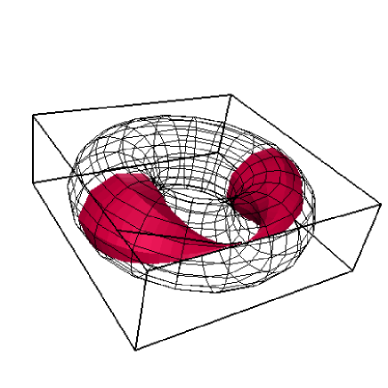
Figure 1. The Maslov cycle $\cal C_{+}$ inside $Sp(2,{\mathbb{R}})$

This index is invariant under homotopies of paths as long as the endpoints do not leave their stratum. It is therefore natural to define the generalized Conley-Zehnder index for any continuous path $\Psi$ in $Sp(2n,{\mathbb{R}})$ by the right hand side of (12)

(13) $$\mu_{CZ}^{g}(\Psi)=\mu_{Lag}(Graph\>\Psi,\Delta).$$

To show that $\mu_{CZ}^{g}(A)=-n/2$ it suffices – in view of the product property of $\mu_{lag}$ – to consider the case

$$a(t)=\begin{pmatrix}1&\frac{t}{4\pi^{2}}\\ 0&1\end{pmatrix}.$$

This path is shown in figure 1 for $t\in[0,200]$ together with the Maslov cycle (the codimension $1$ algebraic variety with one singular point, which corresponds to ${{\mathchoice{\rm 1\mskip-4.0mul}{\rm 1\mskip-4.0mul}{\rm 1\mskip-4.5mul}{\rm 1\mskip-5.0mul}}}$). Here $Sp(2,{\mathbb{R}})$ is identified with the open full torus using an explicit homeomorphism from [GL]. Full details along with more pictures may be found in [W98], [W99].

To calculate $\mu_{CZ}^{g}(a)$ we use its homotopy invariance. The polar decomposition $a(t)=S(t)R(t)$ gives a unitary path $R(t)=e^{2\pi it}$ homotopic to $a$, where $a(0)={{\mathchoice{\rm 1\mskip-4.0mul}{\rm 1\mskip-4.0mul}{\rm 1\mskip-4.5mul}{\rm 1\mskip-5.0mul}}}$ is preserved. Then connect $R(1)$ to $a(1)$ by a path $B(s)$ without intersecting $\cal C_{+}$ except for the endpoint $B(1)=a(1)$. Following first $R$ and then $B$ represents a path homotopic to $a$ with fixed endpoints. Near $a(1)$ the Maslov cycle is an embedding and we may use the intersection number interpretation of $\mu_{CZ}$ to get a contribution $+1$. At the singular point $a(0)={{\mathchoice{\rm 1\mskip-4.0mul}{\rm 1\mskip-4.0mul}{\rm 1\mskip-4.5mul}{\rm 1\mskip-5.0mul}}}$ of $\cal C_{+}$ we compute the signature of the corresponding crossing form of the path $R$, cf. [RS], which turns out to be $-2$. As both endpoints lie in the Maslov cycle they are weighted by a factor $1/2$ and so

$$\mu_{CZ}^{g}(a)=\frac{1}{2}(-2+1)=-\frac{1}{2}.$$

As it should be, perturbing $a$ to a path $\tilde{a}$ on the other side of $\cal C_{+}$ leads to the same number

$$\mu_{CZ}^{g}(\tilde{a})=\frac{1}{2}(0-1)=-\frac{1}{2}.$$

So all elements of $Crit\>{\cal A}$ do have the same generalized Conley-Zehnder index $-n/2$ (note that this implies that there are no nonconstant trajectories of the negative gradient flow of $\cal A$ between critical points). Moreover, addition of $\frac{1}{2}dim\>Crit\>{\cal A}=\frac{n}{2}$ to $\mu_{CZ}^{g}$ yields the Morse index $0$ of the underlying closed geodesics. Let the Bott-type Floer cochain groups be given by the singular chains in $Crit\>{\cal A}$, where the grading is minus the singular grading

$$CF^{-i}_{a,Bott}(T^{*}T^{n},H,g;{\mathbb{Z}})\;=\;\begin{cases}C_{i}^{sing}(Crit_{a}\>{\cal A})&,-i=-n,\ldots,0\\ 0&,\mbox{else}\end{cases}$$

where $a=2\pi^{2}|k|^{2}={\cal A}(x_{u_{0},k})$. This choice of grading is motivated by the nondegenerate case, cf. appendix A and [W99], [SW]. The coboundary operator $\delta_{F}^{-i}$ is defined to be the singular boundary operator $\partial_{i}^{sing}$ and so the Bott-type Floer cohomology groups

$$HF^{-i}_{a,Bott}(T^{*}T^{n},H,g;{\mathbb{Z}}) = \frac{ker\>\delta^{-i}_{F}}{im\>\delta^{-i-1}_{F}}\;,\;i\in{\mathbb{Z}}\;.$$

are given by

$$HF^{-i}_{a,Bott}(T^{*}T^{n},H,g;{\mathbb{Z}})=H_{i}^{sing}(Crit_{a}\>{\cal A})$$

$$\qquad\qquad=H_{i}^{sing}\left(\bigsqcup\nolimits_{l\in{\mathbb{Z}}^{n},|l|\leq|k|}T^{n};{\mathbb{Z}}_{2}\right)$$

$$\qquad\qquad=\begin{cases}\bigoplus_{l\in{\mathbb{Z}}^{n},|l|\leq|k|}{\mathbb{Z}}^{\binom{n}{i}}&,\;-i=-n,\ldots,0\\ 0&,\;\text{else}\>.\end{cases}$$

Appendix A Perturbations

For simplicity let us consider the case $n=1$ only. The general case then follows by taking product manifolds and direct sums of Morse functions. Moreover, we restrict to the $k^{th}$ connected component $\Lambda_{k}S^{1}$ resp. $\Lambda_{k}T^{*}S^{1}$ of the loop space consisting of loops of winding number $k$. This restriction will be clear from our method of perturbation, which does not work uniformly for all components.

First we are going to destroy the circle degeneracy of a closed geodesic $\gamma_{k,q_{0}}(t)=kt+q_{0}$ (represented as a map from ${\mathbb{R}}/{\mathbb{Z}}$ to itself). We follow the beautiful construction in [CFHW]. The strategy is as follows: Choose a Morse-function $h$ on $\gamma_{k,q_{0}}({\mathbb{R}}/{\mathbb{Z}})={\mathbb{R}}/{\mathbb{Z}}$, e.g. $h(y)=-\cos 2\pi y$, define a time-dependent potential $V$ on $\gamma_{k,q_{0}}({\mathbb{R}}/{\mathbb{Z}})$

$$V(t,\gamma_{k,q_{0}}{\scriptstyle(}s{\scriptstyle)}):=h(ks-kt)=-\cos 2\pi(\gamma_{k,q_{0}}{\scriptstyle(}s{\scriptstyle)}-kt-q_{0})\;.$$

The critical points of the perturbed classical action functional ${\cal I}_{V}(\gamma)=\int_{0}^{1}\frac{1}{2}\mid\dot{\gamma}\mid^{2}-V(t,\gamma)\>dt$ are solutions of

$$0 = -\stackrel{{\scriptstyle\cdot\cdot}}{{\gamma}}(t)-\nabla V(t,\gamma{\scriptstyle(}t{\scriptstyle)})=-\stackrel{{\scriptstyle\cdot\cdot}}{{\gamma}}(t)-\frac{1}{4\pi^{2}}\frac{\partial V}{\partial\gamma}(t,\gamma{\scriptstyle(}t{\scriptstyle)})$$

$$= -\stackrel{{\scriptstyle\cdot\cdot}}{{\gamma}}(t)-\frac{1}{2\pi}\sin 2\pi(\gamma{\scriptstyle(}t{\scriptstyle)}-kt-q_{0})\;.$$

We observe that

$$\gamma^{-}(t) = \gamma_{k,q_{0}}(t)=kt+q_{0}$$

$$\gamma^{+}(t) = \gamma_{k,q_{0}}(t+\frac{1}{2k})=kt+q_{0}+\frac{1}{2}$$

are solutions of (A) corresponding to the minimum and maximum of $h$. Equation (A) may be interpreted as describing a mathematical pendulum with gravity, where the observer rotates with angular velocity $k$. The obvious equilibrium states for $k=0$ ’pendulum up’ (unstable) and ’pendulum down’ (stable) correspond to $\gamma^{-}$ and $\gamma^{+}$. This also holds for general $k$. For the rotating observer however these equilibrium states now appear as rotations. A short calculation shows that ${\cal I}_{V}(\gamma^{-})=2\pi^{2}k^{2}+1$, ${\cal I}_{V}(\gamma^{+})=2\pi^{2}k^{2}-1$ and the Morse index of $\gamma^{-}$ resp. $\gamma^{+}$ (regarded as critical points of ${\cal I}_{V}$) is $1$ resp. $0$: The eigenvalues of the perturbed Jacobi operator acting on $C^{\infty}({\mathbb{R}}/{\mathbb{Z}},{\mathbb{R}})$

$$L_{V}^{\mp}\xi=-\stackrel{{\scriptstyle\cdot\cdot}}{{\xi}}-\frac{1}{4\pi^{2}}\frac{\partial^{2}V}{\partial u^{2}}(t,u=\gamma^{\mp})\xi=-\stackrel{{\scriptstyle\cdot\cdot}}{{\xi}}\mp\xi=\lambda_{l}^{\mp}\xi$$

are given by

$$\lambda_{l}^{\mp}=4\pi^{2}l^{2}\mp 1\;,\;l\in{\mathbb{N}}_{0}\;.$$

Hence $L_{V}^{+}$ has only strictly positive eigenvalues, whereas $L_{V}^{-}$ has exactly one negative eigenvalue of multiplicity one, namely $\lambda_{0}^{-}=-1$. Proposition 2.2 in [CFHW] states that $\gamma^{\mp}$ are the only solutions of (A) in $\Lambda_{k}S^{1}$, i.e. $Crit\>{\cal I}_{V}=\{\gamma^{-},\gamma^{+}\}$ is discrete. Therefore the Bott-type Morse complex reduces to the Morse-Witten complex (cf. [Sch],citeW93,[W95])

$$CM_{i}(\Lambda_{k}S^{1},{\cal I}_{V},g;{\mathbb{Z}}_{2}) = \begin{cases}{\mathbb{Z}}_{2}<\gamma^{+}>&,\;i=0\>,\\ {\mathbb{Z}}_{2}<\gamma^{-}>&,\;i=1\>,\\ 0&,\text{else}\>.\end{cases}$$

The only a priori nontrivial matrix element has the coefficient $n_{2}(\gamma^{-},\gamma^{+})$, which is defined to be the number of connecting orbits modulo $2$, i.e. solutions $w\in C^{\infty}({\mathbb{R}}\times{\mathbb{R}}/{\mathbb{Z}},{\mathbb{R}})$ of

(15) $$\partial_{s}w-\partial_{t}\partial_{t}w-\nabla V(t,w)=0\;,\;w(s,\cdot)\stackrel{{\scriptstyle s\rightarrow\mp\infty}}{{\longrightarrow}}\gamma^{\mp}(\cdot)\;.$$

Here we identify two solutions $w,\tilde{w}$, if there exists $\tau\in{\mathbb{R}}$ such that $w(s+\tau,t)=\tilde{w}(s,t)$ for all $s,t$. The Ansatz $w(s,t)=kt+q_{0}+\chi(s)$, where $\chi\in C^{\infty}({\mathbb{R}},{\mathbb{R}}/{\mathbb{Z}})$, leads to the ODE

(16) $$\chi^{\prime}(s)={\scriptstyle\frac{1}{2\pi}}\sin 2\pi\chi(s)\;,$$

which has stationary solutions for the initial values

$$\chi_{0}=\chi(s_{0}=0)={\scriptstyle\frac{1}{2}}\; : \;\chi(s)\equiv{\scriptstyle\frac{1}{2}}\;,$$

$$\chi_{0}=\chi(s_{0}=0)=0\; : \;\chi(s)\equiv 0\;.$$

Choosing initial values $\chi_{0}\in(0,{\scriptstyle\frac{1}{2}})$ resp. $\chi_{0}\in({\scriptstyle\frac{1}{2}},1)$ $\chi(s)$ behaves as follows

$$\chi(s)\stackrel{{\scriptstyle s\rightarrow-\infty}}{{\longrightarrow}}0\;,\;\chi(s)\stackrel{{\scriptstyle s\rightarrow+\infty}}{{\longrightarrow}}{\scriptstyle\frac{1}{2}}\;,$$

resp.

$$\chi(s)\stackrel{{\scriptstyle s\rightarrow-\infty}}{{\longrightarrow}}1\;,\;\chi(s)\stackrel{{\scriptstyle s\rightarrow+\infty}}{{\longrightarrow}}{\scriptstyle\frac{1}{2}}\;,$$

showing that our Ansatz yields two connecting orbits between $\gamma^{-}$ and $\gamma^{+}$. As $Ind_{{\cal I}_{V}}\>(\gamma^{-})=1$ there are no others. As a consequence $n_{2}(\gamma^{-},\gamma^{+})=0$ and the generators of the chain complex coincide with the ones of the corresponding homology groups. Note that equation (16) coincides modulo a factor with the gradient flow equation of the Morse function $h$ on ${\mathbb{R}}/{\mathbb{Z}}$. For general $n$ the (nondegenerate) Morse homology groups coincide with (6).

Now we treat the case of Floer homology of $T^{*}S^{1}$ by perturbing the free Hamiltonian by the time-dependent potential $V$ as above:

$$H(t,u,v)={\scriptstyle\frac{1}{2}}({\scriptstyle\frac{v}{2\pi}})^{2}-\cos 2\pi(u-kt-u^{0})\;$$

We fix a solution $x_{k,x^{0}}(t)=(u_{k,u^{0}}{\scriptstyle(}t{\scriptstyle)},v^{0})=(kt+u^{0},4\pi^{2}k)$ of the unperturbed problem (10). Our equation of interest now reads

$$\begin{pmatrix}\dot{u}(t)\\ \dot{v}(t)\end{pmatrix} = \dot{x}(t)=X_{H}(x{\scriptstyle(}t{\scriptstyle)})$$

$$= \begin{pmatrix}v(t)/(2\pi)^{2}\\ -\frac{\partial V}{\partial u}(t,u{\scriptstyle(}t{\scriptstyle)})\end{pmatrix}=\begin{pmatrix}v(t)/(2\pi)^{2}\\ -2\pi\sin 2\pi(u{\scriptstyle(}t{\scriptstyle)}-kt-u^{0})\end{pmatrix}\;.$$

We have two solutions

$$x^{-}(t)=x_{k,x^{0}}(t)=\begin{pmatrix}kt+u^{0}\\ 4\pi^{2}k\end{pmatrix}\;,\;x^{+}(t)=x_{k,x^{0}}(t+\frac{1}{2k})=\begin{pmatrix}kt+u^{0}+\frac{1}{2}\\ 4\pi^{2}k\end{pmatrix}\;,\;$$

which according to [CFHW] Proposition 2.2 are the only ones. Linearizing (A) at $x^{\mp}$ yields

(18) $$\dot{\xi}(t)=-J\nabla_{\xi(t)}\nabla H(x^{\mp})=-JS^{\mp}\xi(t)\;,$$

where

$$S^{\mp}=\begin{pmatrix}\frac{1}{4\pi^{2}}\frac{\partial^{2}H}{\partial u^{2}}(t,x^{\mp})&\frac{1}{4\pi^{2}}\frac{\partial^{2}H}{\partial u\partial v}(t,x^{\mp})\\ 4\pi^{2}\frac{\partial^{2}H}{\partial v\partial u}(t,x^{\mp})&4\pi^{2}\frac{\partial^{2}H}{\partial v^{2}}(t,x^{\mp})\end{pmatrix}=\begin{pmatrix}\pm 1&0\\ 0&1\end{pmatrix}$$

and

$$J=\begin{pmatrix}0&-g^{11}\\ g_{11}&0\end{pmatrix}=\begin{pmatrix}0&\frac{-1}{4\pi^{2}}\\ 4\pi^{2}&0\end{pmatrix}\;.$$

The flow given by (18) is a path $\Phi^{\mp}:[0,1]\rightarrow Sp(2,{\mathbb{R}})$ starting at the identity: $\Phi^{\mp}(t)=e^{-tJS^{\mp}}$. By [SZ] Theorem 3.3 (iv) the Conley-Zehnder index of $\Phi^{\mp}$ is given by

$$\mu_{CZ}(x^{i})=\mu_{CZ}(\Phi^{i})=\nu(S^{i})-n=\begin{cases}-1&,\;i=-\>,\\ 0&,\;i=+\>,\end{cases}$$

where $\nu^{-}(S^{i})$ denotes the number of negative eigenvalues of $S^{i}$ and $n=1$. Therefore

$$\mu_{CZ}(x^{\mp})=-Ind_{{\cal I}_{V}}\>(\gamma^{\mp});$$

a result which has been established in [W99] in the general nondegenerate case. The construction of the Floer cochain complex proceeds as above. Note that it is graded by minus the Morse index and its cohomology has one generator in dimension $-1$ and one in dimension $0$. For general $n$ the Floer cohomology coincides with (2).

References

[AB] Austin D.M., Braam P.J., Morse-Bott theory and equivariant
cohomology in The Floer memorial volume, PM 133, Birkhäuser 1995.
[CFHW] Cieliebak K., Floer A., Hofer H., Wysocki C.,
Applications of symplectic homology II: stability of the action spectrum,
preprint ETH Zürich.
[CZ] Conley C., Zehnder E., Morse type index theory for flows
and periodic solutions for Hamiltonian equations, Comm. Pure Appl. Math.
XXXVII (1984), 207-253.
[Fl] Floer A., Symplectic fixed points and holomorphic
spheres, Comm. Math. Phys. 120 (1989), 575-611.
[GL] Gelfand I.M., Lidskii V.B., On the structure
of the regions of stability of linear canonical systems of differential
equations with periodic coefficients,
Translations A.M.S. (2) 8 (1958), 143-181.
[Kl] Klingenberg W., Lectures on closed geodesics,
Grundlehren der mathematischen Wissenschaften 230, Springer-Verlag 1978.
[RS] Robbin J., Salamon D., The Maslov index for paths,
Topology 32 (1993), 827-844.
[RT] Ruan Y., Tian G., Bott-type symplectic Floer cohomology
and its multiplication structures, Math. Res. Letters 2 (1995), 203–219.
[Sch] Schwarz M., Morse homology, PM 111, Birkhäuser 1993.
[SW] Salamon D., Weber J., -holomorphic curves in cotangent
bundles and Morse theory on the loop space, in preparation.
[SZ] Salamon D., Zehnder E., Morse theory for periodic solutions
of Hamiltonian systems and the Maslov index, Comm. Pure Appl. Math. XLV
(1992), 1303-1360.
[Vi] Viterbo C., Functors and computations in Floer homology with
applications – part II, preprint October 1996.
[W93] Weber J., Der Morse-Witten Komplex, Diplomarbeit am FB Mathematik
der TU Berlin, Februar 1993.
[W95] Weber J., Morse-Ungleichungen, Supersymmetrie und quasiklassischer
Limes, Diplomarbeit am FB Physik der TU Berlin, Februar 1995.
[W98] Weber J., Topology of and the Conley-
Zehnder index, preprint University of Warwick 51/1998.
[W99] Weber J., -holomorphic curves in cotangent bundles
and the heat flow, PhD-thesis TU Berlin 1999.