Fast Hierarchical Clustering and Other Applications of Dynamic Closest Pairs

Abstract

We develop data structures for dynamic closest pair problems with arbitrary distance functions, that do not necessarily come from any geometric structure on the objects. Based on a technique previously used by the author for Euclidean closest pairs, we show how to insert and delete objects from an $n$-object set, maintaining the closest pair, in $O(n\log^{2}n)$ time per update and $O(n)$ space. With quadratic space, we can instead use a quadtree-like structure to achieve an optimal time bound, $O(n)$ per update. We apply these data structures to hierarchical clustering, greedy matching, and TSP heuristics, and discuss other potential applications in machine learning, Gröbner bases, and local improvement algorithms for partition and placement problems. Experiments show our new methods to be faster in practice than previously used heuristics.

[b]  A preliminary version of this paper appeared at the 9th ACM-SIAM Symp. on Discrete Algorithms, San Francisco, 1998, pp. 619-628. Work supported in part by NSF grant CCR-9258355 and by matching funds from Xerox Corp.

Address: Department of Information and Computer Science, University of California, Irvine, CA 92697-3425, eppstein@ics.uci.edu

1 Introduction

Hierarchical clustering has long been a mainstay of statistical analysis, and clustering based methods have attracted attention in other fields: computational biology (reconstruction of evolutionary trees; tree-based multiple sequence alignment), scientific simulation ($n$-body problems), theoretical computer science (network design and nearest neighbor searching) and of course the web (hierarchical indices such as Yahoo). Many clustering methods have been devised and used in these applications, but less effort has gone into algorithmic speedups of these methods.

In this paper we identify and demonstrate speedups for a key subroutine used in several clustering algorithms, that of maintaining closest pairs in a dynamic set of objects. We also describe several other applications or potential applications of the same subroutine, to TSP heuristics, greedy matching, machine learning, Gröbner basis computation, and local optimization methods.

Although dynamic closest pair data structures have been studied in low-dimensional geometric spaces [?; ?; ?; ?; ?; ?; ?], there has been little work on analogous structures in non-geometric spaces, or in spaces where the dimension is so high as to make taking advantage of the geometry difficult. However, there are several obvious approaches to this dynamic closest pair problem. It can be solved by brute force (trivial recomputation) in time $O(n^{2})$ per update with space $O(n)$, or by a priority queue of distances in time $O(n\log n)$ per update and space $O(n^{2})$. If we maintain the closest distance itself, and recompute all distances when we delete one of the two objects forming this distance, we can even achieve average-case time $O(n)$ per update, in a model in which any deletion is equally likely. However, the applications we describe typically repeatedly delete the closest pair, making the performance of this naive algorithm much worse than its average case.

Of these naive methods, brute force recomputation may be most commonly used, due to its low space requirements and ease of implementation. Three hierarchical clustering codes we examined, Zupan’s [?], CLUSTAL W [?], and PHYLIP [?] use brute force. (Indeed, they do not even save space by doing so, since they all store the distance matrix.) Pazzani’s learning code [?] also uses brute force (M. Pazzani, personal communication), as does Mathematica’s Gröbner basis code (D. Lichtblau, personal communication). The clustering code listed by Anderberg [?] is perhaps more interesting: he uses a “nearest neighbor heuristic” in which one stores the index of each row minimum of the distance matrix (the nearest neighbor to each point), and only updates these indices when these minima change. However, this method may still require $O(n^{2})$ time per update in the worst case. Hartigan [?] describes the same nearest-neighbor heuristic, but resorts to brute force in the associated code listing.

The purpose of this paper is to show that much better bounds are possible, using data structures that are simple and likely to be practical. We adapt and simplify a geometric closest pair data structure of the author [?] to apply in our non-geometric setting, and show that it achieves nearly the best time and space bounds above: $O(n\log^{2}n)$ time per update and space $O(n)$. If linear space is required, this represents an order-of-magnitude speedup over known solutions. Further, with quadratic space, we can also improve significantly on the priority queue; we give an algorithm based on a quadtree-like structure in the distance matrix, with time $O(n)$ per update. This last bound is optimal, since in our model any algorithm needs to examine all $n-1$ distances involving each newly inserted object. It remains open whether quadratic space is required to achieve linear time per update.

Along with these theoretical results, we present experimental results on these data structures and some simple modifications of them. In all our experiments, all our new data structures are preferable to brute force, and one (“FastPair”) is always preferable to the nearest-neighbor heuristic. The choice between it and the other new data structures depends on problem type and available memory.

For recent geometric applications of similar closest pair data structures, in problems of dynamic collision detection, offset curve construction, and skeletonization, see [?].

2 Model of Computation

We assume a model in which we maintain a set of objects subject to insertions or deletions. We are also given a bivariate function $d(s,t)$ measuring the distance between objects. This function need not satisfy the triangle inequality or other common properties of distances; indeed, in the Gröbner basis application below the distances are not numbers. We assume only that function values are totally ordered. The task of our data structures is to maintain the pair $s,t$ having the minimum value $d(s,t)$ among all objects in the set. If two pairs have the same minimum value, our algorithms may return either pair.

We assume that each object is stored in constant space, that the distance function can be evaluated in constant time, and that any two distances can be compared in constant time. These assumptions are not necessarily valid for all applications; for instance Cheng and Wallace [?] describe an application of clustering to meteorology, in which the objects consist of very high dimensional vectors. In computational biology applications, objects may consist of long sequences of symbols, and distance evaluations may consist of complicated dynamic programming routines. In these cases our time bounds can be interpreted as numbers of evaluations; alternatively, with an additional $O(n^{2})$ space, we can precompute and store the entire distance matrix.

For the clustering applications we describe, we also assume some means of treating clusters (sets of objects) as objects themselves, and of computing distances between clusters. There is much freedom in determining distances between clusters. These distances need not be the same as the distances between objects, even for clusters consisting of single objects. Zupan [?] describes seven different definitions of distance between clusters, each of which applies to arbitrary objects and distance functions, and each of which can be computed in constant time (with quadratic space to store all cluster distances) by a formula combining the distances between pairs of subclusters. For biological sequence data, distances between clusters may be computed by a multiple sequence alignment that respects previously computed alignments within each cluster [?; ?]. Alternatively, distances may be defined by selecting a cluster member as a representative object or by combining objects to form a representative in some application-specific way (e.g., centroids for vector data; consensus sequences for biological sequence data). The distance between clusters would then be defined to be the distance between their representative objects. The multiple fragment heuristic for traveling salesman tours involves a similar idea in which each cluster is represented by two objects (at either end of the fragment) with the distance between clusters equal to the minimum of four distances between representative objects.

3 Conga Line Data Structure

We now describe the dynamic closest pair data structure from [?], simplified somewhat by maintaining one set of objects instead of two sets, using a naive nearest neighbor searching technique in place of geometric range searching data structures, and relaxing size restrictions on subsets in a partition of the input.

Our data structure consists of a partition of the dynamic set $S$ into $k\leq\log n$ subsets $S_{1}$, $S_{2}$, …, $S_{k}$, together with a digraph $G_{i}$ for each set $S_{i}$. Each digraph $G_{i}$ will consist of the union of a set of directed paths. Initially all objects will be in $S_{1}$ and $G_{1}$ will have $n-1$ edges. $G_{i}$ may contain edges with neither endpoint in $S_{i}$; if the number of edges in all graphs grows to $2n$ we rebuild the data structure by moving all points to $S_{1}$ and recomputing $G_{1}$. As we will show below, the closest pair will be represented by an edge in some $G_{i}$, so we can find this pair by scanning the edges in all graphs. As we modify $S$, we create and merge these subsets $S_{i}$ and associated graphs $G_{i}$. This involves the following steps:

Create $G_{i}$ for a new partition $S_{i}$.

When created, $G_{i}$ will consist of a single path. We choose the first vertex of the path to be any object in $S_{i}$. Then, we extend the path one edge at a time. When the last vertex in the partially created path $P$ belongs to $S_{i}$, we choose the next vertex to be its nearest neighbor in $S\setminus P$, and when the last vertex belongs to $S\setminus S_{i}$, we choose the next vertex to be its nearest neighbor in $S_{i}\setminus P$. We continue until the path can no longer be extended because $S\setminus P$ or $S_{i}\setminus P$ is empty.

Merge partitions.

The update operations described below can cause $k$ to be too large relative to $n$. If so, we choose subsets $S_{i}$ and $S_{j}$ as close to equal in size as possible: more precisely, if $|S_{i}|\leq|S_{j}|$, we choose these two subsets to minimize the size ratio $|S_{j}|/|S_{i}|$. We then merge these two subsets into a single set and create the graph $G_{i}$ for the merged subset as above.

The construction of $G_{i}$ is essentially the nearest neighbor TSP heuristic, however we are using it for a different purpose. The nearest neighbor searches performed when creating $G_{i}$ can be done by a naive algorithm that tests all objects in $S$ or in $S_{i}$. Improvements can be made in geometric applications by applying more sophisticated range search techniques [?; ?]. We are now ready to describe the update operations in this data structure.

To initialize the data structure

Create a new subset $S_{1}$ containing all the initial objects, and create $G_{1}$.

To insert $x$

Create a new subset $S_{k+1}=\{x\}$ in the partition of $S$, create $G_{k+1}$, and merge partitions as necessary until $k\leq\log n$.

To delete $x$

Create a new subset $S_{k+1}$ consisting of all objects $y$ such that $(y,x)$ is a directed edge in some $G_{i}$. Remove $x$ and all its adjacent edges from all the graphs $G_{i}$. Create the graph $G_{k+1}$ for $S_{k+1}$, and merge partitions as necessary until $k\leq\log n$.

Lemma 1

The data structure described above correctly maintains the closest pair in $S$.

Proof 3.1.

Let $(s,t)$ be a closest pair, where $s$ belongs to a subset $S_{i}$ created more recently than the subset containing $t$. Then when $G_{i}$ was created, it contained $s$, so it contained at least one of $(s,t)$. Then if $s$ was the first of two vertices added to the path, it must have chosen as its neighbor either $t$ or a vertex $x$ at least as close to $s$. If it chose $t$, edge $(s,t)$ exists in $G_{i}$. If it chose some $x$, then $x$ can not have been deleted, since that would have caused $s$ to move to a newer $S_{j}$, so $(s,x)$ is at least as good as $(s,t)$ and still exists in $G_{i}$. Similarly if $t$ were chosen first then it would have formed edge $(t,s)$ in $G_{i}$ or $(t,x)$ for some vertex $x$ at least as close to $t$. Again, $x$ could not have been deleted because that would cause $t$ to move to a subset $S_{j}$ created more recently than $S_{i}$. So in all cases $G_{i}$ contains a closest pair.

Lemma 3.2.

The data structure above uses space $O(n)$.

Proof 3.3.

By construction, the graphs together have at most $2n$ edges (we rebuild the data structure if this bound is reached), so they take linear space to store. The partition is also easily maintained in linear space.

Theorem 3.4.

The data structure above maintains the closest pair in $S$ in $O(n)$ space, amortized time $O(n\log n)$ per insertion, and amortized time $O(n\log^{2}n)$ per deletion.

Proof 3.5.

The correctness and space complexity have already been proven above; it remains to prove the time bounds. First, let us analyze the time for a sequence of updates that do not involve rebuilds to the data structure.

We use a potential function argument. Define the potential of set $S_{i}$ to be $n|S_{i}|\log|S_{i}|$, and the potential of the whole data structure to be the sum of the potentials of each subset. This potential is at most $n^{2}\log n$ (the value it would take for a partition consisting of a single set). The amortized time per operation is $T+B-\Delta$, where $T$ is the actual time used, $B$ is the increase in the upper bound $O(n^{2}\log n)$ on the potential, and $\Delta$ is the increase in the potential. Over the course of a sequence of operations, starting from a situation in which the potential equals $B$, the $B$ and $\Delta$ terms in this formula telescope, so the total amortized time for the sequence is at most the total actual time; therefore this method provides a valid bound on amortized time.

Each time we merge two subsets $S_{i}$ and $S_{j}$, the potential increases by

$$\Delta=n|S_{i}|\log{|S_{i}|+|S_{j}|\over|S_{i}|}+n|S_{j}|\log{|S_{i}|+|S_{j}|\over|S_{j}|}.$$

Since $|S_{i}|$ and $|S_{j}|$ must be within a factor of two of each other, the two logarithmic terms are constant and this simplifies to $\Theta(n(|S_{i}|+|S_{j}|))$. Since the path constructed from the merged subsets has size $O(|S_{i}|+|S_{j}|)$, and each edge in the path can be found in linear time, the total time for the merge is $O(n(|S_{i}|+|S_{j}|))$. Therefore any time spent performing merges can be balanced against an increase in the potential function.

Each time we perform an insertion, we create a new set $S_{k+1}$ with zero potential, and perform $O(n)$ work not counting mergers. However, the bound $O(n^{2}\log n)$ on the total potential increases by $O(n\log n)$, and the amortized time for each insertion must also include this potential increase, so the total amortized time per insertion is $O(n\log n)$.

Each time we perform a deletion, we perform $O(n\log n)$ work creating a new subset of at most $\log n$ objects. This work is balanced by a decrease of $O(n\log n)$ in the upper bound on the total potential. Further, the new set $S_{k+1}$ has some positive potential (up to $O(n\log n\log\log n)$). However, When we move these $\log n$ objects to a new set, the potential of each set $S_{i}$ decreases by $\Theta(n\log|S_{i}|)$ per object, and this potential decrease dominates the amortized time bound for each deletion, which is therefore $O(n\log^{2}n)$.

To complete this analysis, we estimate the time spent rebuilding the data structure. Define the excess of graph $G_{i}$ to be $|G_{i}|-2|S_{i}|$. Initially, all points are in $S_{1}$ with a total excess of $-n$. Each time we merge two subsets, the merged graph’s excess becomes nonpositive. The only way to create a positive excess is to move a point out of some $S_{i}$, by deleting some other point sharing an edge with the moved point. Each deletion moves $O(\log n)$ points and thus increases the total excess by $O(\log n)$. Therefore, $O(n/\log n)$ deletions need to be performed before each rebuild and the amortized time per rebuild step is $O(n\log n)$.

4 Quadtree Data Structure

We now describe a simple technique for maintaining the closest pair even more efficiently, if quadratic space is available.

In a nutshell, we recursively subdivide the distance matrix into a quadtree, and maintain the smallest distance within each quadtree square. Each update affects $O(n)$ squares along a row and column of the distance matrix, and we update the distances within each square by looking at each of its four children.

In more detail, assume the objects are numbered $x_{0}$, $x_{1}$, $\ldots$, $x_{n-1}$. To maintain this numbering, when we insert a new object we give it the next highest number. When we delete an object $x_{i}$ we renumber $x_{n-1}$ to have number $i$, so the numbers stay consecutive. (In practice, it may be possible to combine a deletion with a subsequent insertion, and avoid this renumbering step.)

Define subsets consisting of a number of consecutive objects equal to a power of two: $S(i,j)=\{x_{i2^{j}},x_{i2^{j}+1},\ldots,x_{(i+1)2^{j}-1}\}$. Equivalently, let $S(i,0)=\{x_{i}\}$ and define $S(i,j)$ for $j>0$ to be the disjoint union of $S(2i,j-1)$ and $S(2i+1,j-1)$.

Lemma 4.6.

A set of $n$ objects determines at most $2n-1$ distinct sets $S(i,j)$.

Lemma 4.7.

There are $n$ sets $S(i,0)$, each consisting of a single object. Since each $S(i,j)$ is the disjoint union of two smaller sets, the number of sets $S(i,j)$ with cardinality $2^{j}$ is at most half the number of sets with cardinality $2^{j-1}$, so the total number of sets is at most $n+n/2+n/4+\cdots=2n-1$.

Define $D(i,j,k)$ to be the minimum distance between a point in $S(i,j)$ and a point in $S(k,j)$. By the same reasoning as in the proof of the lemma above, the number of these values is at most $n^{2}/2+n^{2}/8+n^{2}/32+\cdots=2n^{2}/3$.

Lemma 4.8.

Each insertion or deletion to the set of objects causes $O(n)$ values $D(i,j,k)$ to change.

Proof 4.9.

We first consider insertion of a new object. This causes $D(i,j,k)$ to change only when one of $S(i,j)$ or $S(k,j)$ contains the inserted object. Since for any $j$ there is exactly one $S(k,j)$ containing the inserted object, the changed values are in one-to-one correspondence with the sets $S(i,j)$ not containing the inserted object. The result follows from Lemma 4.7. The argument for deletions is similar, except that the deletion of one object and renumbering of another causes roughly twice as many changes to $D(i,j,k)$.

Theorem 4.10.

We can maintain the closest pair among a set of $n$ objects in time $O(n)$ per insertion or deletion, and $O(n^{2})$ space.

Proof 4.11.

As shown above, each update causes $O(n)$ changes to the values $D(i,j,k)$ stored by the data structure. Each changed value can be recomputed in constant time, using the formula

$$D(i,j,k)=\min\{D(2i,j-1,2k),D(2i+1,j-1,2k),D(2i,j-1,2k+1),D(2i+1,j-1,2k+1)\},$$

if we perform the recomputation for smaller values of $j$ before larger ones. The closest pair we seek is $D(0,\lceil\log n\rceil,0)$.

5 Hierarchical Clustering Application

Hierarchical clustering is the process of forming a maximal collection of subsets of objects (called clusters), with the property that any two clusters are either disjoint or nested. Equivalently, it can be viewed as forming a rooted binary tree having the objects as its leaves; the clusters then correspond to the leaves of subtrees. See [?; ?; ?; ?] for surveys of the extensive clustering literature. Although top-down [?], incremental [?], and numerical [?] hierarchical clustering methods are known, hierarchical clustering is often performed by a bottom up agglomerative approach. In agglomerative clustering, one defines a distance between pairs of clusters based on the distance between objects; then, starting with $n$ single-object clusters, one repeatedly forms new clusters by merging the closest pair of clusters.

Many variants of agglomerative clustering are known, largely differing in the definition of cluster distances. This issue was discussed in more detail in our section on models of computation. For single-linkage distance, in which the distance between clusters is formed by the closest pair of objects, agglomerative clustering reduces to Kruskal’s minimum spanning tree algorithm, and can be performed in $O(n^{2})$ time and $O(n)$ space by instead applying Prim’s or Boruvka’s algorithm and sorting the MST edges. There has been some recent work on clustering in low-dimensional spaces [?] or with Hamming distances on binary data [?]. But for cluster distances other than single linkage in more general data sets, no such speedups are known to the merging process defined above. Our data structures improve these clustering algorithms by allowing the nearest pair of clusters to be found quickly.

Theorem 5.12.

We can perform bottom-up hierarchical clustering, for any cluster distance function computable in constant time from the distances between subclusters, in total time $O(n^{2})$. We can perform median, centroid, Ward’s, or other bottom-up clustering methods in which clusters are represented by objects, in time $O(n^{2}\log^{2}n)$ and space $O(n)$.

Proof 5.13.

Each step in these clustering algorithms can be performed by finding the closest pair of clusters, deleting these two clusters from the set of objects represented by our closest pair data structure, and inserting a new object representing the new merged cluster.

6 Traveling Salesman Heuristic Application

Since the traveling salesman problem is NP-complete, but has many applications, a number of heuristics have been devised to approximately solve it. Some, such as the nearest neighbor heuristic (discussed above in connection with our low-space closest pair data structure) and the double minimum spanning tree heuristic, can be solved easily in quadratic time and linear space (optimal in our non-geometric model of computation). However, Bentley [?] has shown that these simple techniques are outperformed by other, seemingly harder to compute methods, such as the multiple fragment heuristic: consider all edges one at a time in sorted order, and include an edge if it connects the endpoints of two fragments of tours (connected components of previously added edges).

Theorem 6.14.

We can implement the multiple-fragment heuristic in time $O(n^{2})$ or in time $O(n^{2}\log^{2}n)$ and space $O(n)$.

Proof 6.15.

This can be seen as a type of hierarchical clustering, in which clusters correspond to fragments, and the distance between two clusters is the length of the shortest edge connecting their endpoints. The sequence of edges added by the hierarchical clustering algorithm of Theorem 5.12 is then exactly the same as the sequence added in the multiple fragment method.

Alternatively, instead of maintaining the closest pair among a set of clusters, maintain the set of fragment endpoints, with distance $+\infty$ between endpoints of the same fragment. Each step of the algorithm then consists of selecting the closest pair, deleting one or both of these endpoints (if they belong to nontrivial fragments) and modifying the distance between the endpoints of the combined fragment.

Another TSP heuristic, cheapest insertion [?], maintains a tour of a subset of the sites, and at each step adds a site by replacing an edge of the tour by two edges through the new site. Each successive insertion is chosen as the one causing the least additional length in the augmented tour.

Theorem 6.16.

We can implement the cheapest insertion heuristic in time $O(n^{2})$ or in time $O(n^{2}\log^{2}n)$ and space $O(n)$.

Proof 6.17.

We use our data structures to maintain a set of $n$ objects: the $k$ edges in the tour after the $k$th insertion, and the $n-k$ remaining uninserted sites. The distance between an edge and a site is defined to be the increase in length that would be caused by the corresponding insertion; all other distances are $+\infty$. In this way each successive insertion can be found as the closest pair in this set.

For sites in a vector space or other set for which the distance between sites and edges is well defined, we can similarly implement nearest insertion [?], which inserts the object closest to the current tour. How efficiently we can implement the farthest insertion heuristic remains unclear.

7 Greedy Matching Application

The greedy matching of a set of points, with some distance function, is found by repeatedly selecting and removing the pair of points with minimum or maximum distance, depending on whether one wants a minimum- or maximum-weight matching. This technique was introduced by Reingold and Tarjan [?], who noted that greedy matchings could be constructed in $O(n^{2}\log n)$ time by sorting the set of distances. Since that paper there has been no improvement in the time bounds for greedy matching.

Greedy matching is not a particularly good approximation to the minimum weight matching [?], even in the average case for one-dimensional points [?]. However, for maximum weight matching with non-negative inter-object distances, greedy matching comes within a factor of two of optimal, and may provide a good starting point for augmenting-path based techniques for finding optimal matchings.

Greedy matching may also be appropriate for non-numeric distances for which addition is undefined, since it lexicographically minimizes or maximizes the set of edge weights in the matching.

Theorem 7.18.

We can perform greedy matching in time $O(n^{2}\log^{2}n)$ and space $O(n)$, or in time $O(n^{2})$.

Proof 7.19.

We use the data structures defined above to repeatedly find and delete the closest pair.

8 Other Applications

We now discuss some other potential applications of our data structures, in which the savings they achieve are less easy to quantify.

8.1 Gröbner Bases

We first consider the problem of computing Gröbner bases for polynomial ideals. Buchberger’s Gröbner basis algorithm is a key component of many symbolic algebra systems and has found a large number of applications including computational geometry and robotics [?], automated deduction [?], and combinatorial enumeration [?]. This algorithm takes as input a set $B=\{f_{1},f_{2},\ldots\}$ of polynomials and a term ordering for comparing monomials, and proceeds to modify $B$ in a sequence of steps, in which $S$-polynomials $S(f_{i},f_{j})$ are constructed and added to $B$, and polynomials in $B$ are simplified by subtracting multiples of each other. As the algorithm proceeds, $B$ can grow very large, so space efficiency is crucial. Further, the choice of which $S$-polynomial to form can make a large difference in the algorithm’s efficiency. For this reason, many implementations follow a suggestion of Buchberger to use the normal selection strategy (e.g. see [?, p. 130]): select $f_{i}$ and $f_{j}$ for which the least common multiple of the leading terms of $f_{i}$ and $f_{j}$ is as small as possible in the term ordering. (Other selection strategies have also been proposed [?; ?] and it seems likely that our methods apply as well to them.)

We can easily apply our closest pair data structures to maintain the set $B$ and select the appropriate pair $f_{i}$, $f_{j}$. Distances between members of $B$ can be measured by least common multiples of leading terms; these values, although non-numeric, can be compared by the term ordering. One complication arises, however: once we have processed $S(f_{i},f_{j})$, we do not want to select the same pair again. So, some data structure such as a hash table should be used so we can test whether this $S(f_{i},f_{j})$ has already been computed, and if so modify the distance between $f_{i}$ and $f_{j}$ to $+\infty$. Such a modification can performed as efficiently as an insertion in our linear-space data structure: simply move $f_{i}$ and $f_{j}$ to a new subset in the partition of the objects maintained by the data structure. In our quadtree data structure, no hash table is needed and modification of a single distance is even easier, taking time $O(\log n)$.

However, pair selection forms a small part of the runtime of Buchberger’s algorithm (D. Lichtblau, personal communication) so improvements would likely have to be made elsewhere to make it worthwhile to implement our data structures for this application.

It may also be of interest to consider applying our techniques to other pair-combination methods of automated deduction such as resolution-based theorem proving.

8.2 Constructive Induction

A second potential application arises in machine learning. Constructive induction is a technique for synthesizing new attributes for multi-attribute data, by combining pairs of attributes. This method can be used to enhance learning methods that can not represent such combinations directly, or that are based on an assumption of attribute independence that may not hold in the actual input. For example, Pazzani [?] forms new attributes from Cartesian products of pairs of discrete-valued attributes, and demonstrates improvements to the learning abilities of Bayesian and nearest-neighbor classification systems. In Pazzani’s experiments, each new product attribute is chosen greedily, as the one that leads to the biggest improvement as measured by leave-one-out cross-validation. Such greedy pairwise combination again seems a natural application for our data structures, but we can only apply them if the quality of an attribute combination stays stable while we insert or delete unrelated attributes. According to Pazzani (personal communication), this stability does hold in practice.

8.3 Non-Hierarchical Clustering

Duran and Odell [?, p. 23] describe a non-hierarchical clustering procedure due to Ball and Hall [?], to which our methods may also apply. In this procedure, a clustering is improved by repeatedly merging the closest pair of clusters (measured by average squared distance) and splitting the cluster with the highest variance. Clearly, our data structures can be used for the merge step, but it is not clear whether this is a significant part of the overall complexity of the algorithm, which also includes “$K$-means”-like phases in which clusters are reconstructed by moving objects to the nearest cluster centroid.

8.4 Local Optimization

Local search procedures such as two-optimization are a common method for improvement of heuristic solutions to optimization problems such as parts placement, traveling salesman tours, or graph partitioning. In these procedures, one modifies a suboptimal solution by moving a small number of objects; the “two-” in two-optimization refers to the number of objects moved. So, for instance, in graph partitioning, one maintains a correct partition while improving the number of crossing edges, by swapping one vertex on one side of the partition for a vertex on the other side; in the traveling salesman problem, one maintains a correct tour while improving its length by removing two edges and replacing them by two other edges connecting the same four vertices. Our methods can likely be used in some of these problems, to maintain the pair of objects the replacement of which leads to the greatest improvement in the objective function.

However, in practice, local optimization is often combined with techniques such as simulated annealing, which randomly selects local changes and allows the objective function to become worse in an attempt to escape local minima. It is not clear how techniques for maintaining the best local improvement should be combined with this simulated annealing approach. Further, application of our ideas to e.g. TSP two-optimization is complicated by the fact that only one of the two ways of replacing a pair of edges will lead to another valid tour; it is not clear whether our data structure can be modified to deal with this additional complication, or with similar complications arising in other problems.

9 Implementation and Experiments

9.1 Algorithms Implemented

In order to test our data structures, we implemented them in a testbed of four algorithms: greedy matching, the multi-fragment TSP heuristic, the cheapest insertion TSP heuristic, and hierarchical clustering by unweighted medians (UPGMA).

We implemented several methods for generating random objects: uniformly distributed vectors with various distance functions (including dot product as well as the more familiar $L_{1}$, $L_{2}$, and $L_{\infty}$ metrics), hierarchically clustered points (via a generalization of the Sierpinski tetrahedron fractal), random leaves of a large binary tree, and random distance matrices. Each object generator allowed all distances to be negated, forming a maximization rather than minimization problem.

The data structures we implemented included our own conga line and quadtree methods, brute force , and the “nearest neighbor heuristic” suggested by authors including Anderberg [?]. In this method, we store each point’s nearest neighbor; closest pairs can be found by scanning this list of neighbors. Insertions can be performed in $O(n)$ time by computing the nearest neighbor to the inserted point and testing whether it should become the nearest neighbor of any other point. However, when a point is deleted, any other point for which it is nearest neighbor must find a new neighbor; if the deleted point was neighbor to $k$ other points, the neighbor heuristic takes time $O(kn)$. If deletions are random or the points belong to a low dimensional metric space, $k=O(1)$ and the time per update is $O(n)$, but it is not hard to find examples in which the worst case time per update is $\Theta(n^{2})$. We did not implement the priority queue method due to its complexity, high space usage and expected poor performance.

In all the methods we implemented, nearest neighbors were computed by a naive sequential scan through all points. In many applications, nearest neighbors can be computed more quickly by heuristics such as spiral search; however we did not implement this due to its complexity. We believe that faster searching would equally speed up brute force, the neighbor heuristic, and our conga line based methods, so adding such heuristics should not change our overall experimental conclusions except possibly by making the quadtree method (which can not use fast neighbor-finding methods) appear worse.

Fig. 1: Hierarchical clustering in ${\bf R}^{20}$. Points were placed uniformly at random in the unit hypercube and clustered by unweighted medians.

Fig. 2: Hierarchical clustering in a 31-dimensional fractal. Points were placed uniformly at random in a generalized Sierpinski tetrahedron formed by choosing 5 random binary values and taking bitwise exclusive ors of each nonempty subset, and clustered by unweighted medians.

Fig. 3: Greedy matching of points placed uniformly at random in the unit hypercube in ${\bf R}^{20}$.

Fig. 4: Greedy matching of points with pseudorandom distances. The distance between two points was computed by using their indices to modify the seed for the drand48 random number generator.

Fig. 5: Greedy maximum-weight matching of points placed uniformly at random in the unit square, with the $L_{1}$ metric.

Fig. 6: Cheapest insertion heuristic for TSP of points placed uniformly at random in a 20-dimensional hypercube.

Fig. 7: Most expensive insertion heuristic for MAXTSP of points placed uniformly at random in the unit square, with the $L_{1}$ metric.

Fig. 8: Multifragment heuristic for TSP of points placed uniformly at random in the unit hypercube in ${\bf R}^{20}$.

Fig. 9: Multifragment heuristic for MAXTSP of points placed uniformly at random in the unit square, with the $L_{1}$ metric.

9.2 Simplified Data Structures: MultiConga

Our conga line implementation includes a parameter $k$ for the number of subsets into which to partition the objects. For best results in our theoretical analysis, $k$ should be $\Theta(\log n)$; our implementation’s default is $k=\log_{2}n$. Our initial expectation was that multiplying this default by a small constant might lead to small improvements, but that non-logarithmic values would cause the time to blow up. To our surprise, the data structure became faster as $k$ grew very large, until the number of distance computations stabilized but the overhead of maintaining many subsets slowed down the structure.

In retrospect, we can explain this heuristically: if $k$ is large, we do few merges of existing subsets, reducing the amortized time per insertion. Although the worst case number of points moved to a new subset by each deletion is $k$, the expected number (if any deletion is equally likely) is $O(1)$ regardless of the number of subsets, so increasing $k$ could typically cause less harm than our worst case analysis would suggest.

With this experience and heuristic justification, we decided to try a modified version of the conga line structure, which we call the “multiple-subset conga line” or “MultiConga” for short. In this structure, we simply never merge subsets $S_{i}$; instead, whenever an insertion or deletion creates a new subset we let the total number of subsets grow. More formally, we modify the conga line data structure operations as follows.

To initialize the data structure

Create a new subset $S_{1}$ containing all the initial objects, and create $G_{1}$.

To insert $x$

Create a new subset $S_{i}=\{x\}$ in the partition of $S$, and create $G_{i}$ (consisting of a single edge from $x$ to its nearest neighbor).

To delete $x$

Create a new subset $S_{i}$ consisting of all objects $y$ such that $(y,x)$ is a directed edge in some $G_{j}$. Remove $x$ and all its adjacent edges from all the graphs $G_{j}$. Create the graph $G_{i}$ for $S_{i}$.

In our experiments, this variant of our closest pair data structure was usually faster than the original conga line data structure, sometimes much faster than the neighbor heuristic, and only rarely slightly slower than the neighbor heuristic. We can provide theoretical evidence for its speed:

Theorem 9.20.

The MultiConga method described above correctly maintains the closest pair in amortized time $O(n)$ per insertion and $O(n^{3/2})$ per deletion.

Proof 9.21.

Correctness follows from the correctness of the conga line data structure. To prove the time bound, we use a potential function $\varphi=\sum_{i}|S_{i}|^{2}n^{1/2}.$ Each insertion changes this potential by $n^{1/2}$ and takes time $O(n)$. Each deletion in which $k$ points are moved to a new subset takes time $O(kn)$, but increases $\varphi$ by $k^{2}n^{1/2}-O(n^{3/2})$. For any $k$, the amortized time (actual time minus difference in $\varphi$) is $O(kn-k^{2}n^{1/2}+n^{3/2})=O(n^{3/2})$.

Although one can concoct examples in which this worst-case bound is tight, we did not find any natural problem for which this method achieved its worst case.

9.3 Simplified Data Structures: FastPair

Since the expected number of points moved into a cluster on each deletion is small, we decided to try a further simplification. In the “FastPair” method, like MultiConga, we never merge subsets. But further, in the case that a deletion would cause $k$ points to move from their current subsets to a new subset, we instead form $k$ singleton subsets. More formally, we have the following two operations:

To initialize the data structure

Create a new subset $S_{1}$ containing all the initial objects, and create $G_{1}$.

To insert $x$

Create a new subset $S_{i}=\{x\}$ in the partition of $S$, and create $G_{i}$ (consisting of a single edge from $x$ to its nearest neighbor).

To delete $x$

Create a separate new subset $S_{i}=\{y\}$ for each object $y$ such that $(y,x)$ is a directed edge in some $G_{j}$. Remove $x$ and all its adjacent edges from all the graphs $G_{j}$. Create the graph $G_{i}$ for each newly created subset $S_{i}$.

The advantage of this data structure compared to the previous ones is that each object $x$ has an outgoing edge to a neighbor only within the set to which it belongs. Therefore, the actual data stored in the structure need only consist of the weight of this outgoing edge and the identity of the neighbor it points to. The partition of the objets into subsets $S_{i}$ does not need to be stored explicitly, as it is not used by the update operations. In addition, the number of edges in the structure is always at most $n$, so we need not worry about rebuilding when the number of edges grows too large.

This FastPair data structure closely resembles the nearest neighbor heuristic, in which again each point remembers a single neighbor. However in the FastPair heuristic the stored neighbor may not always be nearest. In the initial construction of the data structure, instead of computing nearest neighbors for each point, we construct a single conga line, in order to maintain some control over the number of incoming edges per object. And, when inserting a new point, we compute its nearest neighbor as before, but we do not change the stored neighbors of other points even if the newly inserted point is nearer than these stored neighbors. Like the nearest neighbor heuristic, the FastPair method takes linear expected time for random deletions, but has a quadratic worst case. In our experiments, FastPair was always faster than the neighbor heuristic.

9.4 Experimental Results

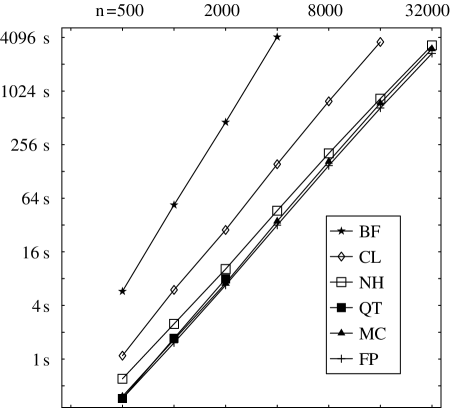
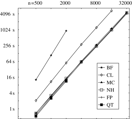
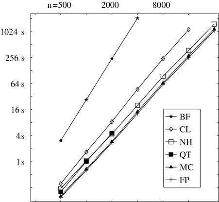
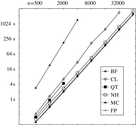
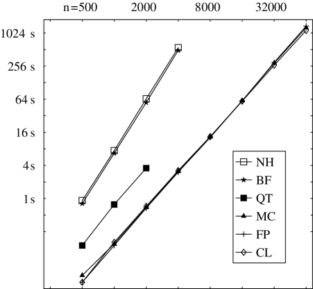
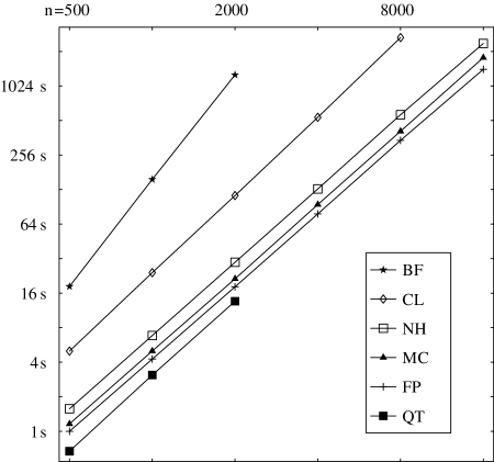
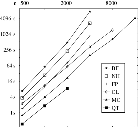
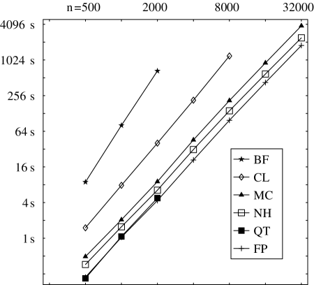
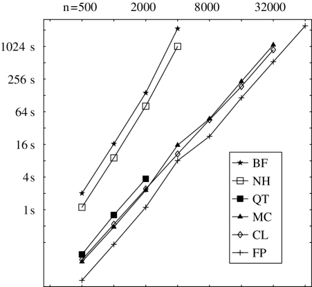
Log-log charts of timing results from our computational experiments are presented in Figures 1–9. In the figures, “BF” stands for the brute force method, “NH” for the neighbor heuristic, “QT” for our quadtree method, “CL” for the basic conga line method, “MC” for MultiConga, and “FP” for FastPair. The times include only the construction of the closest pair data structure and algorithm execution (not initial point placement) and are averages over ten runs. The algorithms were implemented in C$\mathord{+}\mathord{+}$, compiled and optimized by Metrowerks Codewarrior 10, and run on a 200MHz PowerPC 603e processor (Apple Powerbook 3400c). The quadtree data structure was limited to 1000 points by its high memory requirements; other data structures were tested up to the point where a larger input would not fit comfortably into an overnight test run.

We ran one representative application (greedy matching) using a variety of distance functions, and ran a selection of other applications on two distance functions for which our data structures exhibited strikingly different qualitative behavior (Euclidean closest pairs for uniformly generated points in ${\bf R}^{20}$, and rectilinear farthest pairs for uniformly generated points in the unit square). For hierarchical clustering, we also ran a further test on a point set with a fractal structure, to test whether the behavior we observed on uniform points could be assumed to hold also for more realistic clustered data.

Each application performed linearly many updates, so linear time per update translates to quadratic total time in our tests, and quadratic time per update translates to cubic total time. Asymptotic runtime can be estimated by examining the change in running time when doubling the problem size; if the time increases by a factor of four, it can be estimated as quadratic or nearly quadratic, while if the time increases by a factor of eight, it can be estimated as cubic. Due to caching and other issues, it was common for times to increase by factors larger than the theoretical worst case bound, but in general all experiments gave results consistent with cubic or quadratic runtimes.

As expected, brute force always gave cubic runtimes. The neighbor heuristic was often quadratic, but on some problems was cubic, even sometimes slower than brute force. FastPair was also sometimes quadratic, and sometimes cubic; however it was the only method to consistently run faster than the neighbor heuristic (sometimes by a linear factor). The remaining methods always exhibited quadratic behavior (although MultiConga could theoretically have a slower worst case) but sometimes differed by factors of three or more in total runtime. The quadtree method was surprisingly slow; although it performed few distance computations, it was generally only faster than other methods for problems with expensive distance computations. The basic conga line method was often slower by a factor of three to five than its simplifications, and on some problems this factor seemed to be increasing with $n$, perhaps showing that the logarithmic factors in its theoretical time bound were active in practice.

Our conclusion would be to use the quadtree method for problems with few points and slow distance computations; to use FastPair for most applications (after testing to verify that it behaves well for the given application) and to use MultiConga or occasionally the original Conga Line structure when FastPair is known to behave poorly or when a more robustly fast method is required.

The problem of caching remains interesting. The methods we tested involve sequential scans through memory, a behavior known to reduce the effectiveness of cached memory. Some effects of this appear in our data; for instance the last two rows of the brute force data structure for most expensive rectilinear insertion exhibit a jump in runtime by a factor of 15, much higher than the factor of 8 indicated by the asymptotic analysis. We believe that this jump is due to exceeding the limits of the 32Kbyte level I cache on the 603e processor; other jumps can be attributed to exceeding the Powerbook 3400’s 256K level II cache.

The fact that the original Conga Line data structure is slower than MultiConga and FastPair for rectilinear greedy maximum matching with moderate input sizes, even though it performs fewer distance computations, may be due to its higher space usage causing poor caching behavior; note that the other two methods become slower than it only on problem sizes at which they too exceed the cache. Perhaps the relatively poor performance of the quadtree method is also due to its high memory usage. It would be of interest to develop more cache-efficient closest pair data structures which take better advantage of modern computer memory systems.

References

- Adams and Loustaunau (1994) Adams, W. W. and Loustaunau, P. 1994. An Introduction to Gröbner Bases. Number 3 in Graduate Studes in Mathematics. AMS.
- Agarwala et al. (1998) Agarwala, R., Bafna, V., Farach, M., Narayanan, B., Paterson, M. S., and Thorup, M. 1998. On the approximability of numerical taxonomy (fitting distances by tree metrics). SIAM J. Computing 28, 3, 1073–1085.
- Aichholzer (1997) Aichholzer, O. 1997. Combinatorial & Computational Properties of the Hypercube – New Results on Covering, Slicing, Clustering and Searching on the Hypercube. Ph. D. thesis, Tech. Univ. Graz.
- Anderberg (1973) Anderberg, M. R. 1973. Cluster Analysis for Applications. Number 19 in Probability and Mathematical Statistics. Academic Press, New York.
- Ball and Hall (1965) Ball, G. H. and Hall, D. J. 1965. ISODATA, a novel method of data analysis and pattern classification. Technical report, Stanford Research Inst.
- Bentley (1990) Bentley, J. L. 1990. Experiments on traveling salesman heuristics. In Proc. 1st Symp. Discrete Algorithms (January 1990), pp. 91–99. ACM and SIAM.
- Buchberger (1987) Buchberger, B. 1987. Applications of Gröbner bases in non-linear computational geometry. In R. Janßen Ed., Proc. Int. Symp. Trends in Computer Algebra, Number 296 in Lecture Notes in Computer Science (Berlin, May 1987), pp. 52–66. Springer-Verlag.
- Cheng and Wallace (1993) Cheng, X. and Wallace, J. M. 1993. Cluster analysis of the northern hemisphere wintertime 500-hPa height field: spatial patterns. J. Atmospheric Sciences 50, 16 (August), 2674–2696.
- Clegg et al. (1996) Clegg, M., Edmonds, J., and Impagliazzo, R. 1996. Using the Groebner basis algorithm to find proofs of unsatisfiability. In Proc. 28th Symp. Theory of Computing (May 1996), pp. 174–183. ACM.
- Corpet (1988) Corpet, F. 1988. Multiple sequence alignment with hierarchical clustering. Nucleic Acids Research 16, 22, 10881–10890.
- Czapor (1991) Czapor, S. 1991. A heuristic selection strategy for lexicographic Gröbner bases? In Proc. Int. Symp. Symbolic & Algebraic Computation (July 1991), pp. 39–48. ACM.
- Dobkin and Suri (1991) Dobkin, D. and Suri, S. 1991. Maintenance of geometric extrema. J. ACM 38, 275–298.
- Duran and Odell (1974) Duran, B. S. and Odell, P. L. 1974. Cluster Analysis: A Survey. Number 100 in Lecture Notes in Economics and Mathematical Systems. Springer-Verlag, Berlin.
- Eppstein (1995) Eppstein, D. 1995. Dynamic Euclidean minimum spanning trees and extrema of binary functions. Discrete & Computational Geometry 13, 1 (January), 111–122.
- Eppstein and Erickson (1999) Eppstein, D. and Erickson, J. 1999. Raising roofs, crashing cycles, and playing pool: applications of a data structure for finding pairwise interactions. Discrete & Computational Geometry 22, 4, 569–592.
- Felsenstein (1995) Felsenstein, J. 1995. PHYLIP (Phylogeny Inference Package) version 3.572c. Distributed by the author.
- Frieze et al. (1990) Frieze, A., McDiarmid, C., and Reed, B. 1990. Greedy matching on the line. SIAM J. Computing 19, 4 (August), 666–672.
- Giovini et al. (1991) Giovini, A., Mora, T., Niesi, G., Robbiano, L., and Traverso, C. 1991. ‘One sugar cube, please’ or selection strategies in the Buchberger algorithm. In Proc. Int. Symp. Symbolic & Algebraic Computation (July 1991), pp. 49–54. ACM.
- Golin et al. (1998) Golin, M., Raman, R., Schwarz, C., and Smid, M. 1998. Randomized data structures for the dynamic closest-pair problem. SIAM J. Computing 27, 4 (August), 1036–1072.
- Gotoh (1994) Gotoh, O. 1994. Further improvements in methods of group-to-group sequence alignment with generalized profile operations. CABIOS 10, 4, 379–387.
- Hartigan (1975) Hartigan, J. A. 1975. Clustering Algorithms. John Wiley & Sons, New York.
- Krznaric and Levcopoulos (1998) Krznaric, D. and Levcopoulos, C. 1998. Fast algorithms for complete linkage clustering. Discrete & Computational Geometry 19, 1 (January), 131–145.
- Matias (1993) Matias, Y. 1993. Semi-dynamic closest-pair algorithms. In Proc. 5th Canad. Conf. Computational Geometry (August 1993), pp. 264–271.
- Pazzani (1997) Pazzani, M. J. 1997. Constructive induction of Cartesian product attributes. Manuscript.
- Reingold and Tarjan (1981) Reingold, E. M. and Tarjan, R. E. 1981. On a greedy heuristic for complete matching. SIAM J. Computing 10, 4 (November), 676–681.
- Rosenkrantz et al. (1977) Rosenkrantz, D. H., Stearns, R. E., and Lewis, P. M., II. 1977. An analysis of several heuristics for the traveling salesman problem. SIAM J. Computing 6, 3 (September), 563–581.
- Schwarz et al. (1994) Schwarz, C., Smid, M., and Snoeyink, J. 1994. An optimal algorithm for the on-line closest pair problem. Algorithmica 12, 1 (July), 18–29.
- Smid (1992) Smid, M. 1992. Maintaining the minimal distance of a point set in polylogarithmic time. Discrete & Computational Geometry 7, 415–431.
- Sturmfels (1996) Sturmfels, B. 1996. Gröbner Bases and Convex Polytopes. Number 8 in University Lecture Ser. AMS.
- Supowit (1990) Supowit, K. J. 1990. New techniques for some dynamic closest-point and farthest-point problems. In Proc. 1st Symp. Discrete Algorithms (1990), pp. 84–90. ACM and SIAM.
- Thompson et al. (1994) Thompson, J. D., Higgins, D. G., and Gibson, T. J. 1994. CLUSTAL W: improving the sensitivity of progressive multiple sequence alignment through sequence weighting, positions-specific gap penalties and weight matrix choice. Nucleic Acids Research 22, 4673–4680.
- Yianilos (1993) Yianilos, P. N. 1993. Data structures and algorithms for nearest neighbor search in general metric spaces. In Proc. 4th Symp. Discrete Algorithms (January 1993), pp. 311–321. ACM and SIAM.
- Zupan (1982) Zupan, J. 1982. Clustering of Large Data Sets. Chemometrics Research Studies Ser. Research Studies Press, Chichester.