Abstract

We solve the subgraph isomorphism problem in planar graphs in linear time, for any pattern of constant size. Our results are based on a technique of partitioning the planar graph into pieces of small tree-width, and applying dynamic programming within each piece. The same methods can be used to solve other planar graph problems including connectivity, diameter, girth, induced subgraph isomorphism, and shortest paths.

Communicated by Roberto Tamassia: submitted December 1995, revised November 1999.

Work supported in part by NSF grant CCR-9258355 and by matching funds from Xerox Corp.

1 Introduction

Subgraph isomorphism is an important and very general form of exact pattern matching. Subgraph isomorphism is a common generalization of many important graph problems including finding Hamiltonian paths, cliques, matchings, girth, and shortest paths. Variations of subgraph isomorphism have also been used to model such varied practical problems as molecular structure comparison [2], integrated circuit testing [10], microprogrammed controller optimization [26], prior-art avoidance in genetic evolution of circuits [33], analysis of Chinese ideographs [27], robot motion planning [34], semantic network retrieval [36], and polyhedral object recognition [44].

In the subgraph isomorphism problem, given a “text” $G$ and a “pattern” $H$, one must either detect an occurrence of $H$ as a subgraph of $G$, or list all occurrences. For certain choices of $G$ and $H$ there can be exponentially many occurrences, so listing all occurrences can not be solved in subexponential time. Further, the decision problem is NP-complete. However for any fixed pattern $H$ with $\ell$ vertices, both the enumeration and decision problems can easily be solved in polynomial $O(n^{\ell})$ time, and for some patterns an even better bound might be possible. Thus one is led to the problem of determining the algorithmic complexity of subgraph isomorphism for a fixed pattern.

Here we consider the special case in which $G$ (and therefore $H$) are planar graphs, a restriction naturally occurring in many applications. We show that for any fixed pattern, planar subgraph isomorphism can be solved in linear time. Our results extend to some other problems including vertex connectivity, induced subgraph isomorphism and shortest paths.

Our algorithm uses a graph decomposition method similar to one used by Baker [6] to approximate various NP-complete problems on planar graphs. Her method involves removing vertices from the graph leaving a disjoint collection of subgraphs of small tree-width; in contrast we find a collection of non-disjoint subgraphs of small tree-width covering the neighborhood of every vertex.

We assume throughout that all planar graphs are simple, so that the number of edges is at most $O(n)$; this simplifies our time bounds as we need not include the dependence on this number. The only problems for which this assumption makes a difference are induced subgraph isomorphism, $h$-clustering, and edge connectivity; for those, one can assume without loss of generality that the graph has bounded edge multiplicity, so again $m=O(n)$.

2 New Results

We prove the following results. The time dependence on $H$ is omitted from these bounds. In general it is exponential (necessarily so, unless P=NP, since planar subgraph isomorphism is NP-complete) but see Theorem 3 for situations in which it can be improved.

• We can test whether any fixed pattern $H$ is a subgraph of a planar graph $G$, or count the number of occurrences of $H$ as a subgraph of $G$, in time $O(n)$.

• If connected pattern $H$ has $k$ occurrences as a subgraph of a planar graph $G$, we can list all occurrences in time $O(n+k)$. If $H$ is 3-connected, then $k=O(n)$ [16], and we can list all occurrences in time $O(n)$.

• We can count the number of induced subgraphs of a planar graph $G$ isomorphic to any fixed connected pattern $H$ in time $O(n)$, and if there are $k$ occurrences we can list them in time $O(n+k)$.

• For any planar graph $G$ for which we know a constant bound on the diameter, we can compute the exact diameter in time $O(n)$.

• For any constant $h$ we can solve the $h$-clustering and connected $h$-clustering problems [30] in planar graphs in time $O(n)$.

• For any planar graph $G$ for which we know a constant bound on the girth, we can compute the exact girth in time $O(n)$. The same bound holds if instead of girth we ask for the shortest separating cycle or for the shortest nonfacial cycle in a given plane embedding of the graph.

• For any planar graph $G$, we can compute the vertex connectivity and edge connectivity of $G$ in time $O(n)$. (For planar multigraphs, we can test $k$-edge-connectivity for any fixed $k$ in time $O(n)$.)

• For any planar graph $G$ and any constant $\ell$, we construct in time $O(n)$ a linear-space routing data structure which can test for any pair of vertices whether their distance is at most $\ell$, and if so find a shortest path between them, in time $O(\log n)$.

3 Related Work

For general subgraph isomorphism, nothing better than the naive exponential $O(n^{|H|})$ bound is known. Plehn and Voigt [41] give an algorithm for subgraph isomorphism which in planar graphs takes time $|H|^{O(|H|)}n^{O(\sqrt{|H|})}$ (since improved by Alon et al. [1] to $2^{O(|H|)}n^{O(\sqrt{|H|})}$), but this is still much larger than the linear bound we achieve.

Several papers have studied planar subgraph isomorphism with restricted patterns. It has long been known that if the pattern $H$ is either $K_{3}$ or $K_{4}$, then there can be at most $O(n)$ instances of $H$ as a subgraph of a planar graph $G$, and that these instances can be listed in linear time [7, 28, 40], a fact which has been used in algorithms to test connectivity [35], to approximate maximum independent sets [7], and to test inscribability [14]. Linear time and instance bounds for $K_{3}$ and $K_{4}$ can be shown to follow solely from the sparsity properties of planar graphs [12, 13], and similar methods also generalize to problems of finding $K_{2,2}$ and other complete bipartite subgraphs [12, 17]. Richards [42] gives $O(n\log n)$ algorithms for finding $C_{5}$ and $C_{6}$ subgraphs in planar graphs, and leaves open the question for larger cycle lengths; Alon et al. [1] gave $O(n\log n)$ deterministic and $O(n)$ randomized algorithms for larger cycles. In [16], we showed how to list all cycles of a given fixed length in outerplanar graphs, in linear time (see also [37, 38, 39, 45] for similar variants of outerplanar subgraph isomorphism). We used our outerplanar cycle result to find any wheel of a given fixed size in planar graphs, in linear time. Itai and Rodeh [28] discuss the problem of finding the girth of a general graph, or equivalently that of finding short cycles. The problem of finding cycles in planar graphs was discussed above. Fellows and Langston [20] discuss the related problem of finding a path or cycle longer than some given length in a general graph, which they solve in linear time for a given fixed length bound. The planar dual to the shortest separating cycle problem has been related by Bayer and Eisenbud [8] to the Clifford index of certain algebraic curves. Our results here generalize and unify this collection of previously isolated results, and also give improved dependence on the pattern size in certain cases.

Recently we were able to characterize the graphs that can occur at most $O(n)$ times as a subgraph isomorph in an $n$-vertex planar graph: they are exactly the 3-connected planar graphs [16]. However our proof does not lead to an efficient algorithm for 3-connected planar subgraph isomorphism. In this paper we use different techniques which do not depend on high-order connectivity.

Laumond [35] gave a linear time algorithm for finding the vertex connectivity of maximal planar graphs. Eppstein et al. [19] give an $O(n)$ time algorithm for testing $k$-edge-connectivity for $k\leq 4$ and $k$-vertex-connectivity for $k\leq 3$. For general graphs, testing $k$-edge-connectivity for fixed $k$ takes time $O(m+n\log n)$ [25]. 4-vertex-connectivity in general graphs can be tested in time $O(n\alpha(n)+m)$ [29]. However planar graphs can be as much as 5-vertex-connected, and nothing even close to linear was known for testing planar 5-connectivity.

Our shortest path data structure combines our methods of bounded tree-width decomposition with a separator-based divide and conquer technique due to Frederickson [21]. Obviously all pairs shortest paths can be computed in time $O(nm)$ after which the queries we describe can be answered in time $O(1)$, but some faster algorithms are known for approximate planar shortest paths [23, 24, 31]. Our data structure answers shortest path queries exactly, in less preprocessing time than the other known results, but can only find paths of constant length.

A final note of caution is in order. One should not be confused by the superficial similarity between the subgraph isomorphism problems posed here and the graph minor problems studied extensively by Robertson, Seymour, and others [43]. One can recognize path subgraphs by minor testing, but such tricks do not work for most other subgraph isomorphism problems. The absence of a fixed minor imposes severe structural constraints on a graph, whereas this is much less the case when a fixed subgraph is not present. Although minor testing can be done in time polynomial in the text graph size, the constant factors are typically much higher than those for our subgraph isomorphism algorithm.

4 Bounded Tree-Width Subgraph Isomorphism

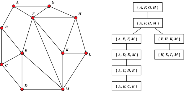
Figure 1: Tree decomposition of a planar graph.

As a subroutine, we need to perform subgraph isomorphism testing in graphs of bounded tree-width. This can be done by a standard dynamic programming technique [9, 46]. The exact statement of the problem we solve is complicated by the requirement that we count or list each subgraph isomorph exactly once. For simplicity, we state the bounds for this problem with one parameter measuring both the tree-width of the text and the size of the pattern.

Definition 1

A tree decomposition of a graph $G$ consists of a tree $T$, in which each node $N\in T$ has a label $L(N)\subset V(G)$, such that the set of tree nodes whose labels contain any particular vertex of $G$ forms a contiguous subtree of $T$, and such that any edge of $G$ connects two vertices belonging to the same label $L(N)$ for at least one node $N$ of $T$. The width of the tree decomposition is one less than the size of the largest label set in $T$. The tree-width of $G$ is the minimum width of any tree decomposition of $G$.

We can assume without loss of generality (by splitting high-degree nodes into multiple nodes with the same label) that each node in $T$ has at most three neighbors and that there are $O(n)$ nodes in the tree. We will assign our tree decomposition an arbitrary orientation, by rooting it at one of its leaves, so that $T$ becomes a binary tree. Figure 1 shows a planar graph, with a tree decomposition of width three. In fact, the graph shown has no tree decomposition of width two, so its tree-width is three.

Define the subtree rooted at a node $N$ to consist of $N$ and all its descendants. Each such subtree is associated with an induced subgraph of $G$, having vertices contained in labels of nodes in the subtree.

Lemma 1

The subtree rooted at $N$ provides a tree decomposition of the associated induced subgraph of $G$.

Proof: The only property of a tree decomposition that does not follow immediately is the requirement that each edge connect two vertices contained in the label of some node. Since this is true of $G$ and $T$, any induced subgraph edge $(u,v)$ must have $\{u,v\}\subset L(N^{\prime})$ for some $N^{\prime}$, but $N^{\prime}$ may not be a descendant of $N$. However, if not, $u$ belongs to both $L(N^{\prime})$ and (by assumption) $L(N^{\prime\prime})$ where $N^{\prime\prime}$ is a descendant of $N$. Therefore, by contiguity, $u\in L(N)$, and similarly $v\in L(N)$, so in this case $(u,v)$ still both belong to the label of at least one node in the subtree. $\Box$

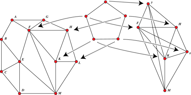
Figure 2: Partial isomorph of a pentagon in the induced subgraph associated with node $\{F,H,K,M\}$, and corresponding partial isomorph boundary mapping the pentagon to $G^{\prime}_{N}$.

Lemma 2

Assume we are given graph $G$ with $n$ vertices along with a tree decomposition $T$ of $G$ with width $w$. Let $S$ be a subset of the vertices of $G$, and let $H$ be a fixed graph with at most $w$ vertices. Then in time $2^{O(w\log w)}n$ we can count all isomorphs of $H$ in $G$ that include some vertex in $S$. We can list all such isomorphs in time $2^{O(w\log w)}n+O(kw)$, where $k$ denotes the number of isomorphs and the term $kw$ represents the total output size.

Proof: We perform dynamic programming in tree $T$. Let a partial isomorph at a node $N$ of the tree be an isomorphism between an induced subgraph $H^{\prime}$ of the pattern $H$ and the induced subgraph of $G$ associated with the subtree rooted at $N$.

We let $G^{\prime}_{N}$ be formed by adding two additional vertices $x$, $y$ to the subgraph of $G$ induced by vertex set $L(N)$. We connect each of the two additional vertices to all vertices in $L(n)$, and each of the two additional vertices also is given a self-loop. Then from any partial isomorph at $N$ we can derive a graph homomorphism from all of $H$ to $G^{\prime}$, which is one-to-one on vertices in $L(N)$, maps the rest of $H^{\prime}$ to $x$, and maps $H-H^{\prime}$ to $y$. Let a partial isomorph boundary be such a map; Figure 2 illustrates a partial isomorph and the corresponding boundary. Since a partial isomorph boundary consists of a map from a set of at most $w$ objects to a set of at most $w+3$ objects, there are at most $w^{w+3}=2^{O(w\log w)}$ possible partial isomorph boundaries for a given node.

Suppose that node $N$ has children $N_{1}$ and $N_{2}$ We say that two partial isomorph boundaries $B:H\mapsto G^{\prime}_{N}$ and $B_{1}:H\mapsto G^{\prime}_{N_{1}}$ are consistent if the following conditions all hold:

• For each vertex $v\in H$, if $B(v)\in L(N_{1})$ or $B_{1}(v)\in L(N)$, then $B(v)=B_{1}(v)$.

• For each vertex $v\in H$, if $B(v)\neq x$ then $B_{1}(v)\in L(N)\cup\{y\}$.

• At least one vertex $v\in H$ has $B_{1}(v)\not\in L(N)\cup\{y\}$.

We say that two partial isomorph boundaries $B_{1}:H\mapsto G^{\prime}_{N_{1}}$ and $B_{2}:H\mapsto G^{\prime}_{N_{2}}$ form a compatible triple with $B$ if the following conditions both hold:

• $B_{1}$ and $B_{2}$ are both consistent with $B$.

• For each $v$ with $B(v)=x$, exactly one of $B_{1}(v)$ and $B_{2}(v)$ is equal to $y$.

For each partial isomorph boundary $B:H\mapsto G^{\prime}_{N}$, let $X_{1}(B)$ be the number of partial isomorphs which give rise to that boundary, and include a vertex of $S$. Let $X_{2}(B)$ be the number of partial isomorphs which give rise to that boundary, and do not include a vertex of $S$. These values can be computed in a bottom-up fashion as follows:

• If there is no $v$ for which $B(v)=x$, then all partial isomorphs having boundary $B$ involve only vertices in $L(N)$, and can be enumerated by brute force in time $2^{O(w\log w)}$.

• Otherwise, we initialize $X_{1}(B)$ and $X_{2}(B)$ to zero. Then, for each partial boundary $B_{1}$ that is consistent with $B$, and such that there is no $v$ with $B(v)=x$ and $B_{1}(v)=y$, we increment $X_{1}(B)$ by $X_{1}(B_{1})$ and increment $X_{2}(B)$ by $X_{2}(B_{1})$. Finally, for each compatible triple $B,B_{1},B_{2}$ we increment $X_{1}(B)$ by $X_{1}(B_{1})\cdot X_{1}(B_{2})+X_{1}(B_{1})\cdot X_{2}(B_{2})+X_{2}(B_{1})\cdot X_{1}(B_{2})$ and increment $X_{2}(B)$ by $X_{2}(B_{1})\cdot X_{2}(B_{2})$.

The total time for testing all triples for compatibility and performing the above computation is $O(w^{3(w+3)+1}=2^{O(w\log w)}$.

At the root node of the tree, we compute the number of isomorphs involving $S$ simply by summing the values $X_{2}(B)$ over all partial isomorph boundaries for which $B(v)\neq y$ for all $v$. $\Box$

Lemma 3

Assume we are given graph $G$ with $n$ vertices along with a tree decomposition $T$ of $G$ with width $w$. Let $S$ be a subset of the vertices of $G$, and let $H$ be a fixed graph with at most $w$ vertices. Then we can list all isomorphs of $H$ in $G$ that include some vertex in $S$ in time $2^{O(w\log w)}n+O(kw)$, where $k$ denotes the number of isomorphs and the term $kw$ represents the total output size.

Proof: We first follow the above dynamic programming procedure, to compute the values $X_{1}$ and $X_{2}$ for each partial isomorph boundary. We then compute top-down in the tree the set of pairs $(B,X)$ where $B$ is a partial isomorph boundary and $X$ is either $X_{1}$ or $X_{2}$, such that the value $X(B)$ contributes to the final count of subgraph isomorphs. These pairs can be identified as the ones such that $X(B)$ was included in the computation of some pair higher in the tree that has been previously identified as contributing to the total, and that caused a nonzero increment in this computation. Finally, we compute bottom-up again, listing for each contributing pair $(B,X)$ the partial subgraph isomorphs counted in the value $X(B)$. This step can be performed by mimicking the initial computation of $X(B)$ described in the previous lemma, restricted to the boundaries known to contribute to the overall total, replacing each increment by a concatenation of lists, and replacing each multiplication with the construction of partial isomorphs from a Cartesian product of two previously-computed lists.

The number of steps for this computation is proportional to the number of steps in the previous algorithm, together with the added time for each combination of a pair of partial isomorphs. Each such combination can be charged to a subgraph isomorph included in the output, and each output isomorph is formed by a binary tree of combinations that takes $O(w)$ time to perform, so the total added time is $O(kw)$. $\Box$

The same dynamic programming techniques also lead to similar results for counting or listing induced subgraphs isomorphic to $H$. To do this, we need only modify the algorithms above to restrict attention to partial isomorph boundaries $B:H\mapsto G^{\prime}_{N}$ in which all edges between vertices of $L(N)$ are covered by the image of some edge in $H$.

5 Neighborhood Covers

We have seen above that we can perform subgraph isomorphism quickly in graphs of bounded tree-width. The connection with planar graphs is the following:

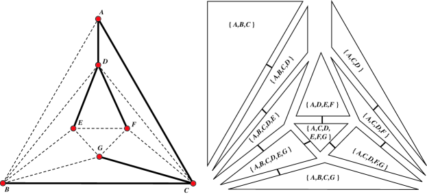
Figure 3: Triangulated planar graph, with depth two tree $T$ rooted at $A$ (shown by heavy solid lines), and tree decomposition with nodes corresponding to faces of the graph and edges complementary to $T$.

Lemma 4 (Baker [6])

Let planar graph $G$ have a rooted spanning tree $T$ in which the longest path has length $\ell$. Then a tree decomposition of $G$ with width at most $3\ell$ can be found in time $O(\ell n)$.

Proof: Without loss of generality (by adding edges if necessary) we can assume $G$ is embedded in the plane with all faces triangles (including the outer face). Form a tree with one node per triangle, and an edge connecting any two nodes whenever the corresponding triangles share an edge that is not in $T$ (Figure 3). Label each node with the set of vertices on the paths connecting each corner of the triangle to the root of the tree. Then each edge’s endpoints are part of some label set (namely, the sets of the two triangles containing the edge), and the labels containing any vertex form a contiguous subtree (namely, the path of triangles connecting the two triangles containing the edge from the vertex to its parent, and any other triangles enclosed in the embedding by this path). Therefore, this gives us a tree decomposition of $G$. The number of nodes in any label set is at most $3\ell+1$, so the width of the decomposition is at most $3\ell$. $\Box$

In particular, any planar graph with diameter $D$ has tree-width $O(D)$.

If an isomorph of a connected pattern $H$ uses vertex $v$ in $G$, it is contained in the portion of $G$ within distance $|H|$ of $v$. By Lemma 4 this $|H|$-neighborhood of $v$ has tree-width at most $3|H|$. Therefore we can cover $G$ by the collection of all such neighborhoods, and use Lemma 3 to find the copies of $H$ within each neighborhood. However such a cover is not efficient: the total size of all subgraphs is $O(n^{2})$, so this would give us a subgraph isomorphism algorithm with quadratic runtime. We speed this up to linear by using more efficient covers.

Awerbuch et al. [3, 5] have introduced the very similar concept of a neighborhood cover, which is a covering of a graph by a collection of subgraphs, with the properties that the neighborhood of every vertex is contained in some subgraph, and that every subgraph has small diameter. They showed that for any (possibly nonplanar) graph, and any given value $w$, there is a $w$-neighborhood cover in which the diameter of each subgraph is $O(w\log n)$, and in which the total size of all subgraphs is $O(m\log n)$; such a cover can be computed in time $O(m\log n+n\log^{2}n)$ [4]. Because of Lemma 4, such a neighborhood cover is also almost exactly what we want to speed up our subgraph isomorphism algorithm. However there are two problems. First, the size and construction time of neighborhood covers are higher than we want (albeit only by polylogarithmic factors). Second, and more importantly, the diameter of each subgraph is logarithmic, so we are unable to use dynamic programming directly in the subgraphs of the cover. We would instead be forced to use some additional techniques such as separator-based divide and conquer, introducing more unwanted logarithmic factors.

Instead, we use a technique similar to that of Baker [6] to form a cover that has the properties we want directly: any connected $w$-vertex subgraph of $G$ is included in some member of the cover, and each vertex of $G$ is included in few members of the cover (so the total size of the cover is $O(n)$). Unlike the techniques cited above, the diameter of the subgraphs will not be bounded, however we will still be able to use Lemma 4 on an auxiliary graph to show that each covering subgraph has tree-width $O(w)$. Because of the exponential dependence of our overall algorithms on the tree-width of the covering subgraphs, we concentrate our efforts on reducing this width as much as possible, at the expense of increasing the total size of the cover by an $O(w)$ factor over the minimum possible.

Lemma 5

Let $G$ be a planar graph, and $w$ be a given integer parameter. Then we can find a collection of subgraphs $G_{i}$ and a partition of the vertices of $G$ into subsets $S_{i}$ with the following properties:

• Every vertex of $G$ is included in at most $w$ subgraphs $G_{i}$.

• We can find a tree decomposition of each subgraph $G_{i}$ with tree-width at most $3w-1$.

• If $H$ is a connected $w$-vertex subgraph of $G$, and $i$ is the smallest value for which $H\cap S_{i}$ is nonempty, then $H$ is a subgraph of $G_{i}$ but is not a subgraph of any $G_{j}$ with $j>i$.

• The total time for performing the partition and computing the tree decompositions is $O(w^{2}n)$.

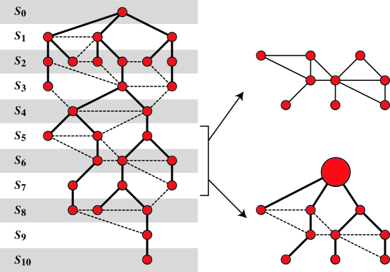
Figure 4: Planar graph with breadth first spanning tree (heavy edges), partition into layers $S_{i}$, subgraph $G_{i}$ (for $w=3$, $i=5$), and minor $G^{\prime}_{i}$ (with large supervertex and contracted breadth first spanning tree).

Proof: We choose an arbitrary starting vertex $v_{0}$, and let $S_{i}$ consist of the vertices at distance $i$ from $v_{0}$. We then let $G_{i}$ be the graph induced by the vertex set $\bigcup_{j=i}^{i+w-1}S_{j}$, as shown in Figure 4. Clearly, the sets $S_{i}$ form a partition of the vertices of $G$, and each vertex is in at most $w$ subgraphs $G_{i}$.

Then for $i=0$, $G_{i}$ consists of the vertices at distance at most $w-1$ from $v_{0}$, so by applying Lemma 4 to its breadth first spanning tree we can find a tree decomposition with width at most $3(w-1)$. To show that each $G_{i}$ with $i>0$ has low tree-width, form an auxiliary graph $G^{\prime}_{i}$ from $G$ by collapsing into a single supervertex all the vertices at distance less than $i$ from $v_{0}$, and deleting all the vertices with distance at least $i+w$. $G^{\prime}_{i}$ is a minor of the planar graph $G$ and is therefore also planar. Then similarly collapsing a breadth first spanning tree of $G$ gives a spanning tree of $G^{\prime}_{i}$ with depth at most $w$, so $G^{\prime}_{i}$ has a tree decomposition with width at most $3w$, in which each node of the decomposition includes the collapsed supervertex in its label. $G_{i}$ is formed by deleting this supervertex from $G^{\prime}_{i}$, so we can form a tree decomposition of $G_{i}$ with width at most $3w-1$ by removing the supervertex from the decomposition of $G^{\prime}_{i}$.

Next, we need to show that any connected subgraph $H$ of $G$ with $|H|\leq w$ is contained in $G_{i}$, where $i$ is the smallest value such that $H\cap S_{i}\neq\emptyset$. But $G_{i}$ is formed from $G$ simply by removing the sets $S_{j}$ where $j<i$ or $j\geq i+w$. No $S_{j}$ with $j<i$ can contain a vertex of $H$, or else $i$ would have been smaller. And no $S_{j}$ with $j\geq i+w$ can contain a vertex $v$ of $H$, or else we could find a path of length at most $i+w-1$ from $v_{0}$ to $v$ by concatenating a path in $H$ from some vertex $v_{i}\in S_{i}\cap H$ to $v$ (which has length at most $|H|-1\leq w-1$) with the breadth first tree path from $v_{0}$ to $v_{i}$ (which has length $i$), contradicting the placement of $v$ in $S_{j}$. Therefore, none of the vertices that were deleted from $G$ can belong to $H$, so $H$ remains a subgraph of $G_{i}$.

Finally, the condition that $H$ can not be a subgraph for $G_{j}$ where $j>i$ is clearly true, since no such $G_{j}$ can include any vertex of $S_{i}$.

The time bound is dominated by the time to perform the tree decompositions on the graphs $G^{\prime}_{i}$, which by Lemma 4 is $\sum O(wG_{i})=wO(\sum G_{i})=w(wn)$. $\Box$

6 The Subgraph Isomorphism Algorithm

We first describe the result for the special case of connected patterns.

Theorem 1

We can count the isomorphs or induced isomorphs of a given connected pattern $H$, having $w$ vertices, in a planar text graph $G$ with $n$ vertices, in time $2^{O(w\log w)}n$. If there are $k$ such isomorphs we can list them all in time $2^{O(w\log w)}n+O(wk)$.

Proof: The algorithm consists of the following steps:

1. Apply the method of Lemma 5 to find a partition of the vertices into sets $S_{i}$ associated with graphs $G_{i}$ having low width tree decompositions.

2. For each $i\geq 0$, count or list the subgraph isomorphs of $H$ in $G_{i}$ that involve at least one vertex of $S_{i}$, using the algorithm of Lemma 2 or Lemma 3 respectively.

3. Sum all the counts or concatenate the lists, to get a count or list of the isomorphs in $G$.

By Lemma 5, each isomorph of $H$ in $G$ occurs in exactly one way as an isomorph in $H_{i}$ that involves at least one vertex of $S_{i}$, so the algorithm produces the correct total count or list. The time for the first step is $O(w^{2}n)$, and the time for the last step is $O(n)$, both dominated by the time for the second step which is $\sum 2^{O(w\log w)}|G_{i}|+O(k_{i}w)$, where the $2^{O(w\log w)}$ factor arises by plugging the $3w-1$ treewidth bound of Lemma 5 into the analysis in Lemmas 2 and 3. This can be simplified to $2^{O(w\log w)}(\sum|G_{i}|)+O(\sum k_{i}w)=2^{O(w\log w)}\cdot O(wn)+O(kw)=2^{O(w\log w)}n+O(kw)$. $\Box$

The method so far requires that the pattern be connected. We now describe a general method for handling disconnected patterns. The technique will let us count the number of matching patterns, after which some sort of separator-based divide and conquer can likely be used to find an instance of a matching pattern, but we have been unable to extend this technique to the problem of listing all subgraph isomorphs of a disconnected pattern.

Theorem 2

We can count the isomorphs of any (possibly disconnected) pattern $H$ having at most $w$ of vertices, in a planar text graph $G$ with $n$ vertices, in time $2^{O(w\log w)}n$.

Proof: Let $\#_{G}(H)$ denote the number of isomorphs of $H$ in $G$. Rather than counting the isomorphs of a single pattern, we count the isomorphs of all planar graphs having at most $w$ vertices. There are only $2^{O(w)}$ such graphs [47], so this factor does not change the overall form of our time bound. We order these graphs by the number of connected components, so that when we are processing a particular graph $H$ we can assume we already know the values of $\#_{G}(H^{\prime})$ for every $H^{\prime}$ with fewer components.

Our algorithm them performs the following steps on each graph $H$:

1. If $H$ is connected, compute $\#_{G}(H)$ using the algorithm of Theorem 1.

2. Otherwise, let $H$ be the disjoint union of two subgraphs $H^{\prime}$ and $H^{\prime\prime}$, and let $\#_{G}(H)=\#_{G}(H^{\prime})\cdot\#_{G}(H^{\prime\prime})-\sum k_{i}\#_{G}(H_{i})$, where the sum is over all graphs $H_{i}$ with fewer components than $H$, and $k_{i}$ denotes the number of different ways $H_{i}$ can be formed as the union of $H_{1}$ and $H_{2}$.

The product $\#_{G}(H^{\prime})\cdot\#_{G}(H^{\prime\prime})$ counts the number of ways of mapping $H$ into $G$ such that both $H^{\prime}$ and $H^{\prime\prime}$ are isomorphically mapped but their instances may overlap. The term $\sum k_{i}\#_{G}(H_{i})$ corrects for these overlaps by subtracting the number of overlapped occurrences of each possible type.

The coefficients $k_{i}$ may be computed by brute force enumeration of all possible ways of marking a vertex of $H_{i}$ as coming from $H^{\prime}$, $H^{\prime\prime}$, or both, combined with a planar graph isomorphism algorithm, in time $2^{O(w)}$. Therefore, the overall time taken in the second step of the algorithm is $2^{O(w)}$, independent of $n$, and the total time is dominated by the first step, in which we apply Theorem 1 to $2^{O(w)}$ connected graphs, taking time $2^{O(w\log w)}n$. $\Box$

7 Further Improvements

For certain patterns, such as the wheels, our results can be further improved to reduce the time dependence on $|H|$. Let ${\rm diam}(H)$ denote the diameter of $H$ (i.e., the longest distance between any two nodes), and let $K_{x}(H)$ denote the maximum number of connected components that can be formed by removing at most $x$ nodes from $H$. Note that if the diameter ${\rm diam}(H)$ is small, we can use that value instead of $|H|$ in our neighborhood cover of $G$, reducing the tree-width of the subgraphs $G_{i}$ to $O({\rm diam}(H))$.

Lemma 6

Let $H$ be a given pattern graph, and $N$ be a node of a tree decomposition of graph $G$. Then there are at most $2^{K_{|L(N)|}(H)+|L(N)|\log(|H|+1)}$ different possible partial isomorph boundaries $B:H\mapsto G^{\prime}_{N}$ (as defined in the proof of Lemma 2).

Proof: The map $B$ can be defined by specifying which (if any) vertex of $H$ maps to each vertex in $L(N)$ (using $\log(|H|+1)$ bits per vertex of $L(N)$ to specify this information) and also specifying which of the remaining vertices in $H$ map to the vertex $x$ in $G^{\prime}_{N}$ and which ones map to the vertex $y$. However, it is not possible for the boundary to come from an actual subgraph isomorphism unless each connected component of $H\setminus B^{-1}(L(N))$ is mapped consistently either to $x$ or to $y$, since any path from $x$ to $y$ must pass through a vertex of $L(N)$. So, to finish specifying the boundary, we need only add this single bit of information per component of $H\setminus B^{-1}(L(N))$, and by definition there are at most $K_{|L(N)|}(H)$ such components. $\Box$

As a consequence, the analysis in Lemma 2 can be tightened to show that the dynamic program takes time $2^{O(K_{O(diam(H))}(H)+{\rm diam}(H)\log|H|)}n$.

Lemma 7

Suppose that planar graph $H$ is Hamiltonian, or is 3-connected, or is connected and has bounded degree. Then for any set $S$ of vertices of $H$, $H-S$ has $O(|S|)$ connected components.

Proof: For Hamiltonian graphs and bounded degree graphs this is straightforward. For 3-connected graphs, assume without loss of generality that no edge can be added to $H$ connecting two vertices in $S$; then each component of $H-S$ must occupy a distinct face in the planar embedding of $S$ induced by the unique embedding of $H$. $\Box$

Theorem 3

If a given pattern $H$ is Hamiltonian, 3-connected, or connected of bounded degree, we can count the isomorphs of $H$ in a planar text graph $G$ with $n$ vertices in time $2^{O({\rm diam}(H)\log|H|)}n$.

Proof: The proof consists simply of plugging the improved analysis of Lemma 6 into the algorithm of Theorem 1. $\Box$

For instance we can count the isomorphs of a wheel $W_{k}$ in a planar text graph $G$ with $n$ vertices, in time $O(nk^{O(1)})$. In fact in this case it is not difficult to come up with an $O(nk^{2})$ algorithm:

Theorem 4

We can count the isomorphs of any wheel $W_{k}$ in a planar text graph $G$ with $n$ vertices in time $O(nk^{2})$.

Proof: For each vertex $v$, we count the number of cycles of length $k$ in the neighbors of $v$. The sum of the sizes of all neighborhoods in $G$ is $O(n)$. Each neighborhood has treewidth at most 2 by Lemma 4. Any partial isomorphism of a $k$-cycle in a node $N$ of this decomposition can only consist of a single path of at most $k-1$ vertices, which starts and ends at some two of the at most three vertices in $L(N)$ and may or may not involve the third vertex; therefore we need only keep track of $O(k)$ different partial isomorph boundaries at each node. A careful analysis of the steps in the algorithm of Lemma 2 then shows that the most expensive step (finding compatible triples) can be performed in time $O(k^{2})$ per node, giving an overall running time of $O(k^{2}n)$. $\Box$

8 Variations and Applications

We now describe briefly how to use our subgraph isomorphism algorithm to solve certain other related graph problems. For instance, we can find the girth (shortest cycle), or smallest nonfacial cycle (for some particular embedding) simply by searching for isomorphs of small cycles:

Theorem 5

We can find the girth $g$ of any planar graph $G$, or find a smallest nonfacial cycle $C$ for an embedded planar graph, in time $2^{O(g\log g)}n$ or $2^{O(|C|\log|C|)}n$ respectively.

Proof: We test for each integer $i=3,4,5\ldots$ whether there is a cycle (or nonfacial cycle) of length $i$. To test if there is a nonfacial cycle, we count the total number of cycles of length $i$ in the graph and subtract the number of faces of length $i$. The total time for this procedure is $\sum_{i\leq g}2^{O(i\log i)}n=2^{O(g\log g)}n$. For the nonfacial cycle problem, once the length of the cycle is known, we can find a single such cycle by performing our subgraph isomorph listing algorithm, stopping once $k+1$ cycles are generated, where $k=O(n)$ is the number of faces of the given length. By radix sorting the list of cycles (in lexicographic order by their sequences of vertex indices) we can then test in linear time which of the generated cycles are nonfacial. $\Box$

Theorem 6

We can find a shortest separating cycle $C$ in a planar graph, in time $2^{O(|C|\log|C|)}n$.

Proof: We describe how to test for the existence of a separating cycle of length $i$; the shortest such cycle can then be found by a sequential search similar to the computation of the girth.

We first modify the construction of the graphs $G_{i}$ in Lemma 5, by including in $G_{i}$ not only all the vertices in layers $S_{i}$ through $S_{i+w-1}$ but also a single supervertex for each connected component of the graph induced by the vertices in layers $S_{j}$, $j\geq i+w$, and a supervertex for the (single) connected component of the vertices in layers $S_{j}$, $j<i$. Then a cycle that uses only vertices in layers $S_{i}$ through $S_{i+w-1}$ (and does not use any of the supervertices) is separating in the modified $G_{i}$ if and only if the corresponding cycle is separating in $G$. Note that the added supervertices only add one level to the breadth first search tree of $G_{i}$ and hence the tree-width is still $O(w)$.

Then we need merely modify the dynamic program of Lemma 2, to use a definition of a partial isomorph boundary that, in addition to the map $B:H\mapsto G^{\prime}_{N}$, specifies which of the remaining unmapped vertices of $G^{\prime}_{N}$ are in each of the two subsets of $G$ separated by the cycle, enforcing the requirement that no vertex in one subset be adjacent to a vertex in the other subset. This modification multiplies the number of boundaries by $2^{O(w)}$, but this increase is swamped by the $2^{O(w\log w})$ terms from our previous analysis. $\Box$

We next consider the application of our techniques to certain graph clustering problems.

Definition 2 (Keil and Brecht [30])

The $h$-clustering problem is that of approximating the maximum clique by finding a set of $h$ vertices inducing as many edges as possible. The connected $h$-clustering problem adds the restriction that the induced subgraph be connected.

Keil and Brecht [30] study these problems, and show that even though cliques are easy to find in planar graphs [40], the connected $h$-clustering problem is NP-complete for planar graphs. See [32] for approximate $h$-clustering algorithms in general graphs.

Theorem 7

For any $h$ we can solve the planar $h$-clustering and connected $h$-clustering problems in time $2^{O(h\log h)}n$.

Proof: We simply to test subgraph isomorphism for all possible planar graphs on $h$ vertices, and return the subgraph isomorph with the most edges. $\Box$

We now describe two applications to connectivity that, unlike the previous applications, are linear without an exponential dependence on a separate parameter.

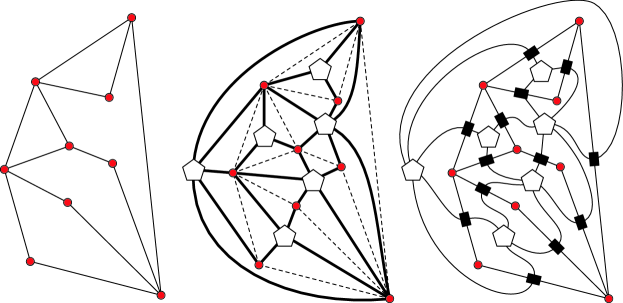
Figure 5: An embedded planar graph $G$, the vertex connectivity substitute graph $G^{\prime}$ (with edges drawn as heavy curves), and the edge connectivity substitute graph $G^{\prime\prime}$.

The vertex connectivity of $G$ is the minimum number of vertices such that their deletion leaves a disconnected subgraph. Since every planar graph has a vertex of degree at most five, the vertex connectivity is at most five. We now use a method of Nishizeki (personal communication) to transform the vertex connectivity problem into one of finding short cycles, similar to those discussed at the start of this section. We choose some plane embedding of $G$, and construct a new graph $G^{\prime}$ having $n+f$ vertices: the $n$ original vertices of $G$ and $f$ new face-vertices corresponding to the faces of $G$. We place an edge in $G^{\prime}$ between an original vertex and a face-vertex whenever the corresponding vertex and face are incident in $G$. Then $G^{\prime}$ is a bipartite plane-embedded graph. This construction is illustrated in the center of Figure 5.

Lemma 8

Any minimal set $S\subset G$ of vertices the deletion of which would disconnect $G$ corresponds to a cycle $C\subset G^{\prime}$ of the same original vertices and an equal number of face-vertices in $G^{\prime}$, such that $G^{\prime}\setminus C$ has at least two connected components each containing at least one original vertex. Conversely if $C$ is any cycle such that $G^{\prime}\setminus C$ has at least two connected components each containing at least one original vertex, then the original vertices in $C$ form a cutset in $G$.

Proof: Let $A$ be a connected component of $G\setminus S$, let $G_{A}$ be formed from $G$ by contracting $A$ into a supervertex, and let $S^{\prime}$ be the set of faces and vertices adjacent to the contracted supervertex. Then (since it is just the neighborhood of a vertex) $S^{\prime}$ has the structure of a cycle in $G^{\prime}$, and separates $A$ from $G\setminus\{A\cup S\}$. If $S$ is minimal, then it must consist of exactly the original vertices in $S^{\prime}$. The converse is immediate, since no edge in the embedding of $G$ can cross a face or vertex in $C$. $\Box$

Theorem 8

We can compute the vertex connectivity of a planar graph in $O(n)$ time.

Proof: We can assume without loss of generality that $G$ is two-connected, so the graph $G^{\prime}$ described in Lemma 8 has no multiple adjacencies. We form $G^{\prime}$ as above and find the shortest cycle in $G^{\prime}$ that separates two original vertices. As with the shortest separating cycle problem (Theorem 6) this can be done by a slight modification to our dynamic programming method that decorates the dynamic programming states with $O(1)$ bits of additional information regarding the separated vertices. Since any planar graph has a vertex of degree at most five by Euler’s formula, the shortest cycle in $G^{\prime}$ must have length at most ten, so the algorithm takes time $O(n)$. $\Box$

The edge connectivity of a graph is similarly defined as the minimum number of edges the removal of which disconnects the graph. For simple graphs, this can again be at most five but for multigraphs it can be higher.

Theorem 9

We can compute the edge connectivity of a simple planar graph in $O(n)$ time.

Proof: Assume without loss of generality that $G$ is two-edge-connected. Embed $G$, and form a graph $G^{\prime\prime}$ by subdividing each edge of $G$ and connecting the resulting subdivision points to new vertices in each adjacent face; this construction is illustrated in the right of Figure 5. Then $G^{\prime\prime}$ is a planar graph with $n$ original vertices, $e$ edge-vertices on each edge of $G$, and $f$ face-vertices in each face of $G$, so its total complexity is $O(n)$. By the assumption of two-edge-connectivity, $G^{\prime\prime}$ is simple. One can use an argument similar to the one in Lemma 8, in which we delete a cutset from $G$, contract a connected component, and examine the neighborhood in $G$ of the contracted supervertex, to show that $G$ is $k$-edge-connected iff there is no cycle of fewer than $2k$ edge- and face-vertices in $G^{\prime\prime}$, which separates two original vertices. As before, the degree bound on a planar graph imposes a limit of ten on the length of the shortest such cycle, and as before this cycle can be found by a minor modification to our dynamic programming algorithm. $\Box$

The same methods extend easily enough to multigraphs, but now the edge connectivity can not be bounded a priori, so we need to include the connectivity in our time bound.

Theorem 10

For any fixed $k$, we can test $k$-edge-connectivity of a planar multigraph in time $2^{O(k\log k)}n$.

Proof: Without loss of generality, the multiplicity of any edge is at most $k$, as higher multiplicities can not improve the overall connectivity. After the edge subdivision step in the construction of $G^{\prime\prime}$, the resulting graph is a simple planar graph with $O(kn)$ vertices, after which we can proceed as in the remainder of Theorem 9. $\Box$

9 Shortest Path Data Structure

We next describe a technique for finding shortest paths in planar graphs. Let a parameter $\ell$ be given (typically, a fixed constant). We wish to test, for any two vertices $u$ and $v$, whether there is a path from $u$ to $v$ of distance at most $\ell$, and if so return the shortest such path.

Since we wish to use an amount of space independent of $\ell$, we need a variant of Lemma 5 in which the total size of the subgraphs is not so large.

Lemma 9

Let $G$ be a planar graph, and $w$ be a given integer parameter. Then we can find a collection of subgraphs $G_{i}$ and a partition of the vertices of $G$ into subsets $S_{i}$ with the following properties:

• Every vertex of $G$ is included in at most two subgraphs $G_{i}$.

• We can find a tree decomposition of each subgraph $G_{i}$ with tree-width $O(w)$.

• $G_{i}$ contains the $\ell$-neighborhood of every vertex in $S_{i}$.

• The total time for performing the partition and computing the tree decompositions is $O(wn)$.

Proof: As in Lemma 5, we compute the distances of each vertex from some arbitrary starting vertex $v_{0}$. We then let $S_{i}$ consist of those vertices with distance at least $2iw$ and at most $(2i+2)w-1$ from $v_{0}$, and we let $G_{i}$ be the graph induced by the set of vertices with distances at least $(2i-1)w$ and at most $(2i+3)w-1$ from $v_{0}$. The proof that these graphs have treewidth $O(w)$ and that each $G_{i}$ contains the $\ell$-neighborhood of $S_{i}$ is essentially the same as that of Lemma 5. $\Box$

As before, by introducing dummy nodes, we can assume without loss of generality that each node in the tree decomposition of $G_{i}$ has at most three neighbors. We warm up with a data structure for our shortest path queries that uses more space than necessary, but for which queries are very fast.

Theorem 11

Given a planar graph $G$, and any value $\ell$, we can in time and space $O(\ell n\log n)$ build a data structure that can, given a query pair of vertices, either return the distance between the pair or determine that the distance is greater than $\ell$, in time $O(\ell)$ per query.

Proof: By performing the decomposition of Lemma 9 we can assume without loss of generality that we have a tree decomposition $T$ for $G$ of width $O(\ell)$. As with any tree, we can find a node $N$ the removal of which disconnects $T$ into subtrees of size at most $|T|/2$. Our primary data structure consists of the distances $d(x,z)$ from each vertex $x\in G$ to each vertex $z\in L(N)$, together with a recursively constructed data structure in each subtree.

To answer a query pair $x,y$ where the two vertices belong to different subtrees of $T$, we can simply try each of the $O(D)$ values $d(x,z)+d(z,y)$ where $z$ ranges over all the members of $L(N)$. To answer a query where the two vertices belong to the same subtree, we can use the recursively defined structure in that subtree.

It remains to show how we quickly determine which node $N$ is eventually used to answer each query. To do this, define the level of a node to be the stage in the recursive subdivision process at which the node was chosen, and define the superior of a node $N$ to be the node chosen at the next earlier level in the subtree containing $N$. The links from a node to its superior define a tree structure $T^{\prime}$ different from the original decomposition tree $T$. Further, define the home node of a vertex $v$ to be the node with the earliest level with $v\in L(N)$. Note that, because of the requirements that the labels containing $v$ are contiguous, the home node is uniquely defined. Then, the node to be used in answering a query pair $x,y$ is simply the least common ancestor in $T^{\prime}$ of the home nodes of $x$ and $y$. $\Box$

To return the actual shortest path, rather than simply the distance between a pair of nodes, we can store a single-source shortest path tree for each member of $L(N)$, and return the path in the tree for the member of $L(N)$ giving the smallest distance.

We next show how to reduce the space to linear, at the expense of increasing the query time.

Theorem 12

Given a planar graph $G$, and any value $\ell$, we can build a data structure of size $O(\ell n)$ that can, given a query pair of vertices, either return the distance between the pair or determine that the distance is greater than $\ell$, in time $O(\ell^{2}\log n)$ per query.

Proof: As above, we can assume $G$ has a tree decomposition of width $O(\ell)$, which we assume has the form of a rooted binary tree. Define levels in this tree and home nodes of vertices as above, except that we terminate the recursive subdivision process when we reach subtrees with fewer than $\ell$ nodes (which we call small subtrees). If the node labels containing a vertex $v$ belong only to nodes in a small subtree $S$, then $v$ does not have a home node, instead we say that $S$ is $v$’s home subtree.

Define a pair of nodes in $T$ to be related if there is no node between them with an earlier level than both. Then, each node $N$ is related to $O(1)$ nodes at each level: one node at an earlier level than $N$, and at most one node in each later level in each of the at most three subtrees formed by removing $N$ from $T$. Therefore, there are $O(n/\ell)$ pairs of related nodes.

Our data structure then consists of the matrix of distances from vertices in $L(N_{1})$ to vertices in $L(N_{2})$, for each pair $N1,N2$ of related nodes. The space for this data structure is $O(n\ell)$. It can either be built as a subset of the data structure of Theorem 11, in time $O(n\ell\log n)$, or bottom-up (using hierarchical clustering techniques of Frederickson [22] to construct the level structure in $T$, and then computing each distance matrix from two previously-computed distance matrices in time $O(\ell^{3})$) in total time $O(n\ell^{2})$; we omit the details.

To answer a query, we form chains of related pairs connecting the home nodes (or small subtrees) of the query vertices to their common ancestor in $T^{\prime}$. The levels of the nodes in these two chains becomes earlier at each step towards the common ancestor, so the total number of pairs in the chain is $O(\log n)$. We then build a graph, in which we include an edge between each pair of vertices in the labels of a related pair of nodes, labeled with the distance stored in the matrix for that pair. We also include in that graph the edges of $G$ belonging to the small subtrees containing the query vertices, if they belong to small subtrees. The query can then be answered by finding a shortest path in this graph, which has $O(\ell\log n+\ell^{2})$ vertices and $O(\ell^{2}\log n)$ edges. $\Box$

The following theorem on computing diameter improves the naive $O(n^{2})$ bound for all pairs shortest paths when the diameter is small. Note that diameter is not a subgraph isomorphism problem but it succumbs to similar techniques.

Theorem 13

We can compute the diameter $D$ of a planar graph $G$, in time $O(2^{O(D\log D)}n)$.

Proof: We begin by performing a breadth first search from an arbitrary vertex. This will produce a tree of height at most $D$, so by Lemma 4 we can find a tree decomposition of width $O(D)$, which as usual we can assume has the form of a rooted binary tree. We first perform a bottom-up sweep of this tree to compute for every node $N$ the distances between every pair of vertices in $L(N)$, in the graph associated with the subtree rooted at $N$. These $O(D^{2})$ distances can be found by combining the distance matrices of the two children of $N$, in time $O(D^{3})$, so this phase takes time $O(D^{3}n)$. We then sweep the decomposition top down, computing for every node $N$ the distances between every pair of vertices in $L(N)$, in the whole graph $G$. The first pass correctly computed these distances at the root of the tree, and at any other node $N$ the distances can be computed by combining the distance matrices of the parent of $N$ (previously computed in the top-down sweep) and its two children (computed in the bottom-up sweep), again in time $O(D^{3})$ per node.

We finally sweep through the tree decomposition bottom up, keeping at each node $N$ a subset $S$ of the vertices seen so far in the subtree rooted at $N$, together with the distances from each member of $S$ to each member of $L(N)$. When we process a node $N$, we perform the following steps:

1. Let the set $S$ for node $N$ consist of the union of the corresponding sets $S_{1}$ and $S_{2}$ for its children $N_{1}$ and $N_{2}$, together with $L(N)$.

2. Compute the distances from each member of $S$ to each member of $L(N)$, by combining the previously computed distances to $L(N_{1})$ or $L(N_{2})$ with the distances within $L(N_{1})\cup L(N_{2})$.

3. Compute the distance between each pair of nodes $x,y$ where $x\in S_{1}\setminus L(N)$ and $y\in S_{2}\setminus L(N)$, by testing the distances through all $O(D)$ possible intermediate nodes in $L(N)$.

4. Radix sort the members of $S$ according to the lexicographic ordering of their $O(D)$-tuples of distances to $L(N)$, and eliminate all but one member for each distinct tuple.

The value returned as the diameter is then the maximum of the distances from $S$ to $L(N)$ computed in the second step, and the distances of pairs $x,y$ comuted in the third step

If any eliminated member $x$ of a tuple belongs to a diametral pair $x,y$, where $y$ is not in the subgraph associated with $N$, then the uneliminated member $x^{\prime}$ with the same tuple would have the same distance to $y$, and would form another diametral pair. Therefore, the algorithm above will correctly find and report a diametral pair.

The number of distinct $O(D)$-tuples of integers in the range from $0$ to $D$ is $2^{O(D\log D)}$, hence this gives a bound on the size of each set $S$. The time to compute distances between pairs $x,y$ is $O(D)$ times the square of this quantity, which is still $2^{O(D\log D)}$. $\Box$

10 Other Graph Families

Our results for planar graphs use the assumption of planarity in two ways. First, in the bound relating tree-width to diameter (Lemma 4), the proof is based on the existence of a planar embedding of the graph, and in fact there is no similar bound in general for nonplanar graphs; for instance the complete graph $K_{n}$ has diameter one but tree-width $n-1$. Second, in the cover of $G$ by low-treewidth subgraphs described in Lemma 5, we needed the fact that planar graphs are closed under minors to show that the graph $G^{\prime}_{i}$ is planar, allowing us to apply Lemma 4 to it.

This naturally raises the question, for which other minor-closed graph families can we prove a bound relating diameter to tree-width, similar to Lemma 4? Such a result would then let us apply our subgraph isomorphism techniques unchanged to any such families. In the conference version of this paper [18], we announced an exact characterization of these families, which are detailed in a separate journal paper [15] and which we now summarize:

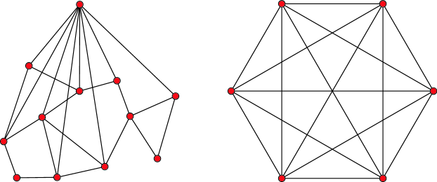
Figure 6: The graph on the left is an apex graph; the topmost vertex is one of the possible choices for its apex. The graph on the right is not an apex graph.

Definition 3

Define a family $\cal F$ of graphs to have the diameter-treewidth property if there is some function $f(D)$ such that every graph in $\cal F$ with diameter at most $D$ has treewidth at most $f(D)$.

Definition 4

An apex graph is a graph $G$ such that for some vertex $v$ (the apex), $G\setminus\{v\}$ is planar (Figure 6).

Theorem 14 ([15])

Let $\cal F$ be a minor-closed family of graphs. Then $\cal F$ has the diameter-treewidth property iff $\cal F$ does not contain all apex graphs.

Corollary 1

Let $\cal F$ be a minor-closed family of graphs, such that some apex graph is not in $\cal F$. Let $H$ be a fixed graph in $\cal F$. Then there is a linear time algorithm for testing whether $H$ is a subgraph of a given graph $G\in\cal F$.

Note that the bound on tree-width from Theorem 14 is much higher than the linear bound in Lemma 4, so the dependence on $|H|$ of the time bound of the algorithm implied by Corollary 1 is much greater than in our planar graph algorithms. However, for certain important minor-closed graph families (such as bounded genus graphs) we were able to prove a better dependence of tree-width on diameter [15], leading to less impractical algorithms.

11 Conclusions and Open Problems

We have shown how to solve planar subgraph isomorphism for any pattern in time $O(n)$. We have also solved certain related problems in similar time bounds. A number of generalizations of the problem remain open:

• We have shown that we can solve planar subgraph isomorphism even for disconnected patterns in time $O(n)$. Can we list all occurrences of a disconnected pattern in time $O(n+k)$?

• Bui and Peck [11] describe an algorithm for finding the smallest set of edges partitioning a planar graph into two sets of vertices with specified sizes; if the edge set has bounded size their algorithm has cubic running time. Can we use our methods to find such a partition more quickly?

• It seems possible that the recently discovered randomized coloring technique of Alon et al. [1] can improve the dependence on the size of the pattern from $2^{O(w\log w)}$ to $2^{O(w)}$, but only for the decision problem of subgraph isomorphism. Can we achieve similar improvements for the counting and listing versions of the subgraph isomorphism problem?

References

- [1] N. Alon, R. Yuster, and U. Zwick. Color-coding. J. Assoc. Comput. Mach. 42(4):844–856, July 1995.
- [2] P. J. Artymiuk, P. A. Bath, H. M. Grindley, C. A. Pepperrell, A. R. Poirrette, D. W. Rice, D. A. Thorner, D. J. Wild, P. Willett, F. H. Allen, and R. Taylor. Similarity searching in databases of three-dimensional molecules and macromolecules. J. Chemical Information and Computer Sciences 32:617–630, 1992.
- [3] B. Awerbuch, B. Berger, L. Cowen, and D. Peleg. Low-diameter graph decomposition is in NC. 3rd Scand. Worksh. Algorithm Theory (SWAT), vol. 621, pp. 83–93. Springer-Verlag Lecture Notes in Computer Science, 1992.
- [4] B. Awerbuch, B. Berger, L. Cowen, and D. Peleg. Near-linear time construction of sparse neighborhood covers. SIAM J. Computing 28(1):263–277, 1998.
- [5] B. Awerbuch and D. Peleg. Sparse partitions. Proc. 31st IEEE Symp. Foundations of Computer Science, pp. 503–513, 1990.
- [6] B. S. Baker. Approximation algorithms for NP-complete problems on planar graphs. J. Assoc. Comput. Mach. 41:153–180, 1994.
- [7] R. Bar-Yehuda and S. Even. On approximating a vertex cover for planar graphs. Proc. 14th Symp. Theory of Computing, pp. 303–309. Assoc. Comput. Mach., 1982.
- [8] D. Bayer and D. Eisenbud. Graph curves. Advances in Math. 86:1–40, 1991.
- [9] M. W. Bern, E. L. Lawler, and A. L. Wong. Linear-time computation of optimal subgraphs of decomposable graphs. J. Algorithms 8:216–235, 1987.
- [10] A. D. Brown and P. R. Thomas. Goal-oriented subgraph isomorphism technique for IC device recognition. IEE Proceedings I (Solid-State and Electron Devices) 135:141–150, 1988.
- [11] T. N. Bui and A. Peck. Partitioning planar graphs. SIAM J. Computing 21:203–215, 1992.
- [12] N. Chiba and T. Nishizeki. Arboricity and subgraph listing algorithms. SIAM J. Computing 14:210–223, 1985.
- [13] M. Chrobak and D. Eppstein. Planar orientations with low out-degree and compaction of adjacency matrices. Theoretical Computer Science 86:243–266, 1991.
- [14] M. B. Dillencourt and W. D. Smith. A linear-time algorithm for testing the inscribability of trivalent polyhedra. Proc. 8th Symp. Computational Geometry, pp. 177–185. Assoc. Comput. Mach., 1992.
- [15] D. Eppstein. Diameter and treewidth in minor-closed graph families. To appear in Algorithmica, math.CO/9907126.
- [16] D. Eppstein. Connectivity, graph minors, and subgraph multiplicity. J. Graph Theory 17:409–416, 1993.
- [17] D. Eppstein. Arboricity and bipartite subgraph listing algorithms. Information Processing Letters 51:207–211, 1994.
- [18] D. Eppstein. Subgraph isomorphism in planar graphs and related problems. Proc. 6th Symp. Discrete Algorithms, pp. 632–640. Assoc. Comput. Mach. and Soc. Industrial & Applied Math., 1995.
- [19] D. Eppstein, Z. Galil, G. F. Italiano, and T. H. Spencer. Separator based sparsification II: edge and vertex connectivity. SIAM J. Computing 28(1):341–381, 1999.
- [20] M. R. Fellows and M. A. Langston. On search, decision and the efficiency of polynomial-time algorithms. Proc. 21st Symp. Theory of Computing, pp. 501–512. Assoc. Comput. Mach., 1989.
- [21] G. N. Frederickson. Fast algorithms for shortest paths in planar graphs, with applications. SIAM J. Computing 16:1004–1022, 1987.
- [22] G. N. Frederickson. Ambivalent data structures for dynamic 2-edge-connectivity and smallest spanning trees. SIAM J. Comput. 26(2):484–538, April 1997.
- [23] G. N. Frederickson and R. Janardan. Efficient message routing in planar networks. SIAM J. Computing 18:843–857, 1989.
- [24] G. N. Frederickson and R. Janardan. Space-efficient message routing in -decomposable networks. SIAM J. Computing 19:14–30, 1990.
- [25] H. N. Gabow. A matroid approach to finding edge connectivity and packing arborescences. J. Computer & System Sciences 50:259–273, 1995.
- [26] A. Guha. Optimizing codes for concurrent fault detection in microprogrammed controllers. Proc. Int. Conf. Computer Design: VLSI in Computers and Processors (ICCD ’87), pp. 486–489. Inst. Electrical & Electronics Engineers, 1987.
- [27] D. Hong, Y. Wu, and X. Ding. An ARG representation for Chinese characters and a radical extraction based on the representation. Proc. 9th Int. Conf. Pattern Recognition, vol. 2, pp. 920–922. Inst. Electrical & Electronics Engineers, 1988.
- [28] A. Itai and M. Rodeh. Finding a minimum circuit in a graph. SIAM J. Computing 7:413–423, 1978.
- [29] A. Kanevsky, R. Tamassia, G. Di Battista, and J. Chen. On-line maintenance of the four-connected components of a graph. Proc. 32nd IEEE Symp. Foundations of Computer Science, pp. 793–801, 1991.
- [30] J. M. Keil and T. B. Brecht. The complexity of clustering in planar graphs. J. Combinatorial Mathematics and Combinatorial Computing 9:155–159, 1991.
- [31] P. N. Klein and S. Sairam. Fully dynamic approximation schemes for shortest path problems in planar graphs. Algorithmica 22(3):235–249, November 1998.
- [32] G. Kortsarz and D. Peleg. On choosing a dense subgraph. Proc. 34th Symp. Foundations of Computer Science, pp. 692–703. Inst. Electrical & Electronics Engineers, 1993.
- [33] J. R. Koza, F. H. Bennett, III, and O. Stiffelman. Genetic programming as a Darwinian invention machine. Proc. 2nd Worksh. Genetic Programming (EuroGP ’99). Springer-Verlag, Lecture Notes in Computer Science 1598, 1999, http://www.genetic-programming.com/EUROGP99.ps.
- [34] S. Y. T. Lang and A. K. C. Wong. A sensor model registration technique for mobile robot localization. Proc. Int. Symp. Intelligent Control, pp. 298–305. Inst. Electrical & Electronics Engineers, 1991.
- [35] J.-P. Laumond. Connectivity of plane triangulations. Information Processing Letters 34:87–96, 1990.
- [36] R. Levinson. Pattern associativity and the retrieval of semantic networks. Computers and Mathematics with Applications 23:573–600, 1992.
- [37] A. Lingas. Subgraph isomorphism for biconnected outerplanar graphs in cubic time. Theoretical Computer Science 63:295–302, 1989.
- [38] A. Lingas and A. Proskurowski. On parallel complexity of the subgraph homeomorphism and the subgraph isomorphism problem for classes of planar graphs. Theoretical Computer Science 68:155–173, 1989.
- [39] A. Lingas and M. M. Sysło. A polynomial-time algorithm for subgraph isomorphism of two-connected series-parallel graphs. Proc. 15th Int. Colloq. Automata, Languages and Programming, pp. 394–409. Springer-Verlag, Lecture Notes in Computer Science 317, 1988.
- [40] C. H. Papadimitriou and M. Yannakakis. The clique problem for planar graphs. Information Processing Letters 13:131–133, 1981.
- [41] J. Plehn and B. Voigt. Finding minimally weighted subgraphs. Proc. 16th Int. Worksh. Graph-Theoretic Concepts in Computer Science, pp. 18–29. Springer-Verlag, Lecture Notes in Computer Science 484, 1991.
- [42] D. Richards. Finding short cycles in planar graphs using separators. J. Algorithms 7:382–394, 1986.
- [43] N. Robertson and P. D. Seymour. Graph Structure Theory: Proc. Joint Summer Res. Conf. Graph Minors. Contemporary Mathematics 147. Amer. Math. Soc., 1991.
- [44] T. Stahs and F. M. Wahl. Recognition of polyhedral objects under perspective views. Computers and Artificial Intelligence 11:155–172, 1992.
- [45] M. M. Sysło. The subgraph isomorphism problem for outerplanar graphs. Theoretical Computer Science 17:91–97, 1982.
- [46] K. Takamizawa, T. Nishizeki, and N. Saito. Linear-time computability of combinatorial problems on series-parallel graphs. J. Assoc. Comput. Mach. 29:623–641, 1982.
- [47] G. Turán. On the succinct representation of graphs. Discrete Applied Mathematics 8(3):289–294, 1984.