Finite-Resolution Hidden Surface Removal

Abstract

We propose a hybrid image-space/object-space solution to the classical hidden surface removal problem: Given $n$ disjoint triangles in $\mathrm{I\!R}^{3}$ and $p$ sample points (“pixels”) in the $xy$-plane, determine the first triangle directly behind each pixel. Our algorithm constructs the sampled visibility map of the triangles with respect to the pixels, which is the subset of the trapezoids in a trapezoidal decomposition of the analytic visibility map that contain at least one pixel. The sampled visibility map adapts to local changes in image complexity, and its complexity is bounded both by the number of pixels and by the complexity of the analytic visibility map. Our algorithm runs in time $O(n^{1+\varepsilon}+n^{2/3+\varepsilon}t^{2/3}+p)$, where $t$ is the output size. This is nearly optimal in the worst case and compares favorably with the best output-sensitive algorithms for both ray casting and analytic hidden surface removal. In the special case where the pixels form a regular grid, a sweepline variant of our algorithm runs in time $O(n^{1+\varepsilon}+n^{2/3+\varepsilon}t^{2/3}+t\log p)$, which is usually sublinear in the number of pixels.

1 Introduction

Hidden surface removal is one of the oldest and most important problems in computer graphics. Informally, the problem is to compute the portions of a given collection of geometric objects, typically composed of triangles, that are visible from a given camera position and orientation in $\mathrm{I\!R}^{3}$. In order to simplify calculation (and explanation), a projective transformation is applied so that the camera is at $-\infty$ on the $z$-axis and all vertices have positive $z$-coordinates, so that the desired image is the orthographic projection of the objects onto the $xy$-plane. We will follow the computer graphics convention that the $y$-axis is vertical, the $x$- and $z$-axes are horizontal, and the positive $z$-axis points into the image, directly away from the camera.

Historically, there are two different approaches to solving the hidden surface removal problem: object space and image space [46]. Object-space (or analytic) hidden surface removal algorithms compute which object is visible at every point in the image plane. Image-space algorithms, on the other hand, compute only the object visible at a finite number of sample points. We will refer to the sample points themselves as “pixels”, since usually there is one sample point per pixel in the final finite-resolution output image. (Image-space algorithms that compute sub-pixel features do so by sampling a small constant number of points within each pixel area [20].)

The output of an object-space hidden surface removal algorithm is the projection of the forward envelope of the objects onto the image plane. The resulting planar decomposition is called the visibility map of the objects. Each face of the visibility map is a maximal connected region in which a particular triangle, or no triangle, is visible. McKenna [38] described the first algorithm to compute visibility maps in $\Theta(n^{2})$ time, where $n$ is the number of input triangles; see also [15]. This is optimal in the worst-case. Unfortunately, McKenna’s algorithm always uses $\Theta(n^{2})$ time and space, even when the visibility map is much simpler. This shortcoming led to the development of several output-sensitive algorithms, whose running time depends not only on $n$, the number of triangles, but also on $v$, the number of vertices of the visibility map. The fastest algorithm currently known, an improvement by Agarwal and Matoušek [2] of an algorithm of de Berg et al. [6], runs in time $O(n^{1+\varepsilon}+n^{2/3+\varepsilon}v^{2/3})$. For more details on these and other object-space algorithms, see the comprehensive survey by Dorward [17].

The primary disadvantage of the object-space approach is the potentially high complexity of the visibility map, which may be much larger than the number of pixels in the desired output image, even for reasonable input sizes. Even when the visibility map is not overly complex, it may contain features that are significantly smaller than the area of a pixel and thus do not contribute to the final image. This is especially problematic for applications of hidden-surface removal such as form-factor calculation, where the desired output image may have very low resolution [45].

For image-space algorithms, on the other hand, the ultimate goal is to compute, for each pixel in the finite-resolution output image, which triangle is visible at that pixel. The most common image-space approach is the $z$-buffer algorithm introduced by Catmull [9]. This algorithm loops through the triangles, determining the pixels that each triangle covers in the image plane; each pixel maintains the smallest $z$-coordinate of any triangle covering that pixel. While this algorithm can be implemented cheaply in hardware, it can still be quite slow when the number of triangles and number of pixels are both large.

Another common image-space approach is ray casting (also known as ray tracing and ray shooting): Shoot a ray from each pixel in the positive $z$-direction and compute the first triangle it hits. Using using the best known unidirectional ray-shooting data structure, due to Agarwal and Sharir [3], we obtain an algorithm with running time $O((n+n^{2/3}p^{2/3}+p)\log^{3}n)$, where $n$ is the number of triangles and $p$ is the number of pixels. Erickson’s lower bound for Hopcroft’s problem [18] suggests that this algorithm is close to optimal in the worst case, even for the simpler problem of deciding whether any ray hits a triangle. In practice, ray-shooting queries are answered by walking through a decomposition of space determined by the triangles, such as an octtree [21], triangulation [4], or binary space partition [40, 42]. See [4, 29] for related theoretical results.

Neither $z$-buffers nor ray casting exploit spatial coherence in the image. If the visible triangles are fairly large, then the same triangle is likely to be visible through several pixels; however, both algorithms compute the triangle behind each pixel independently. Spatial coherence is exploited to some extent by more complex techniques such as Warnock’s subdivision algorithm [49], hierarchical $z$-buffers [23], hierarchical coverage masks [24], and frustum casting [48], which construct a recursive quadtree-like decomposition of the image. However, this decomposition can be much more complex than the visibility map if, for example, the image contains several long diagonal lines. In particular, if the pixels lie in a regular $\sqrt{p}\times\sqrt{p}$ grid, the decomposition can have complexity $\Theta(v\sqrt{p})$.

A few hidden surface removal algorithms work simultaneously in both image and object space [28, 50]. The basic idea for these algorithms is to traverse the objects in order from front to back (i.e., by increasing “distance” from the camera), decomposing the image plane using the boundaries of the objects and reverting to ray casting when any region of the image plane contains only a single pixel. Of course, there are sets of triangles do not have a consistent depth order, and these algorithms will produce incorrect output if such as set is given as input. While a depth order can always be guaranteed by first decomposing the triangles with a binary-space partition tree, this could produce $\Theta(n^{2})$ triangle fragments in the worst case [42]. One exception to the depth-order requirement is Weiler and Atherton’s algorithm [50], which decomposes the image plane into regions within which the triangles can be depth-ordered; this algorithm can also produce a quadratic number of fragments. The image decompositions produced by these algorithms produce cannot be analyzed either in terms of the complexity of the visibility map, since they can decompose triangles even when all depth cycles are invisible, or in terms of the number of pixels, since they can produce many fragments that do not contain a pixel at all.

In this paper, we propose another hybrid approach to hidden surface removal that exploits both spatial coherence and finite precision. In Section 2, we define the sampled visibility map of a set of triangles with respect to a set of pixels. Like other image-decomposition schemes, the sampled visibility map adapts to local changes in the image complexity, but unlike previous approaches its complexity is easily bounded both by the complexity of the analytic visibility map and by the number of pixels.

We describe an output-sensitive algorithm to construct the sampled visibility map in Section 4. Our algorithm runs in time ${O(n^{1+\varepsilon}+n^{2/3+\varepsilon}t^{2/3}+p)}$, where $t$ is the number of trapezoids in the output. This matches the performance of Agarwal and Matoušek’s visibility map algorithm when $t=\Theta(v)$, and almost matches Agarwal and Sharir’s ray-casting algorithm when $t=\Theta(p)$. Our algorithm does not require the triangles to have a consistent depth order, nor does it decompose the triangles into orderable fragments. A variant of our algorithm allows a sequence of pixels to be specified online, at an additional amortized cost of $O(\log t)$ time per pixel.

The algorithms presented in Section 4 assume that the pixels are just arbitrary points in the $xy$-plane. In Section 5, we describe a faster algorithm for the common special case where the pixels are the vertices of a rectangular grid. The running time of our improved algorithm is $O(n^{1+\varepsilon}+n^{2/3+\varepsilon}t^{2/3}+t\log p)$, which is sublinear in the number of pixels unless the output is very large.

Finally, in Section 6, we discuss some other applications of our techniques and suggest directions for further research.

2 Definitions

Let $\Delta$ be a set of $n$ disjoint triangles in $\mathrm{I\!R}^{3}$, where every vertex has positive $z$-coordinate. We say that a triangle $\triangle\in\Delta$ is visible at a point $\pi$ in the $xy$-plane if a ray from $\pi$ in the positive $z$-direction hits $\triangle$ before any other triangle in $\Delta$. The visibility map $Vis(\Delta)$ is a planar straight-line graph, each face of which is a maximal connected region in which a particular triangle in $\Delta$, or no triangle, is visible. See Figure 1(a). Let $v$ denote the number of vertices of $Vis(\Delta)$.

The trapezoidal decomposition of $Vis(\Delta)$, denoted $Trap(Vis(\Delta))$, is obtained by decomposing each face into (possibly degenerate) trapezoids, two of whose edges are vertical (i.e., parallel to the $y$-axis). The vertical edges are defined by casting segments up and/or down from each vertex into the face, stopping when the segment reaches another edge of the face. Faces are decomposed individually, so only one vertical edge is added at a “T” vertex where one visible edge appears to overlap another. See Figure 1(b).

Finally, let $P$ be a set of $p$ points in the $xy$-plane, called “pixels”. The sampled visibility map of $\Delta$ with respect to $P$, denoted ${Vis(\Delta\mid\nobreak P)}$, is the subset of trapezoids in $Trap(Vis(\Delta))$ that contain at least one pixel in $P$. See Figure 1(d). Let $t$ denote the number of trapezoids in ${Vis(\Delta\mid\nobreak P)}$. Clearly $t\leq p$, since every trapezoid in ${Vis(\Delta\mid\nobreak P)}$ contains at least one pixel. Moreover, since $Trap(Vis(\Delta))$ contains at most $2v$ trapezoids, ${t\leq 2v}$.

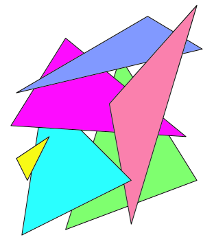
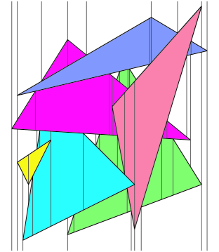
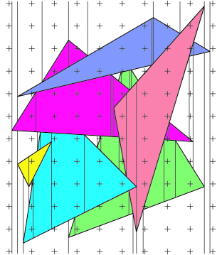
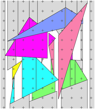
(a) (b) (c) (d)

Figure 1: (a) The visibility map $Vis(\Delta)$ of a set $\Delta$ of triangles, (b) its trapezoidal decomposition $Trap(Vis(\Delta))$, (c) with a grid of pixels $P$, and (d) the resulting sampled visibility map ${Vis(\Delta\mid\nobreak P)}$.

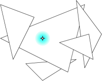
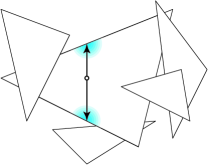
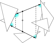
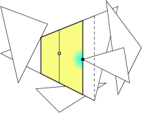
(a) (b) (c) (d)

Figure 2: Building one trapezoid in ${Vis(\Delta\mid\nobreak P)}$. (a) Shoot a ray into the scene through the pixel to the first triangle. (b) Drag rays up and down to find the top and bottom edges. (c) Drag rays along the top and bottom edges to find their (potential) endpoints. (d) Narrow the trapezoid by locating the nearest visible vertices on either side.

3 Building One Trapezoid in ${Vis(\Delta\mid\nobreak P)}$

A naïve algorithm for constructing the sampled visibility map would start by constructing $Vis(\Delta)$. While this approach leads to an algorithm that is nearly optimal in the worst case, it cannot give an output-sensitive algorithm. To obtain output-sensitivity, we construct ${Vis(\Delta\mid\nobreak P)}$ one trapezoid at a time. Specifically, for each pixel $\pi\in P$, if it is unmarked, we determine the trapezoid $\tau_{\pi}\in Trap(Vis(\Delta))$ that contains it and then mark all the pixels contained in $\tau_{\pi}$. We construct each trapezoid in four stages, which are illustrated in Figure 2.

Stage 1. Forward Ray Shooting. The first stage in constructing the trapezoid $\tau_{\pi}$ is to determine the triangle visible at $\pi$; see Figure 2(a). This is done by answering a unidirectional ray-shooting query, exactly as in the standard ray-casting algorithm. Agarwal and Sharir [3] describe a data structure that can answer such queries in time $O((n/\sqrt{s})\log^{3}n)$ using a data structure of size $O(s\log^{2}n)$, where $s$ can be chosen anywhere between $n$ and $n^{2}$. The preprocessing time needed to construct this data structure is $O(s\log^{3}n)$.

Agarwal and Sharir’s data structure is actually designed to answer point stabbing queries for a set of triangles in the plane—How many triangles contain the query point? Like most geometric range searching structures, their data structure defines a number of canonical subsets of the set of triangles. For any point $\pi$, the set of triangles that contain $\pi$ can be expressed as the disjoint union of $O((n/\sqrt{s})\log^{3}n)$ canonical subsets; in particular, this implies that the triangles in any canonical subset have a common intersection. Their data structure stores the size of each canonical subset, and a stabbing query is answered by summing up the sizes of the relevant canonical subsets. To obtain a unidirectional ray-shooting data structure for our three-dimensional triangles $\Delta$, it suffices to build Agarwal and Sharir’s point-stabbing structure for the $xy$-projection of $\Delta$. Now the triangles in any canonical subset have a consistent front-to-back ordering, and the triangle visible through $\pi$ can be computed by comparing the front-most triangles in the relevant canonical subsets.

Stage 2. Vertical Ray Dragging. The second stage in our algorithm finds the top and bottom edges of $\tau_{\pi}$. Intuitively, these edges are computed by dragging the ray through $\pi$ parallel to the $y$-axis until the triangle hit by the ray changes. See Figure 2(b). Let $\triangle_{\pi}\in\Delta$ be the triangle visible at $\pi$, and let $\bar{\pi}$ be the point on $\triangle_{\pi}$ with the same $x$- and $y$-coordinates as $\pi$. (To avoid the case where no triangle is visible at $\pi$, we can assume that there is a large “background” triangle.) Let the curtain of a triangle edge be the set of points on or directly behind that edge; each curtain is a three-sided unbounded polygonal slab, two of whose sides are parallel to the $z$-axis [6]. We can find the top (resp. bottom) edge of $\tau_{\pi}$ by shooting a ray from $\bar{\pi}$ along the surface of $\triangle_{\pi}$ in the positive (resp. negative) $y$-direction. In each case, the desired edge is determined either by an edge of $\triangle_{\pi}$ or by the first curtain hit by the ray. Agarwal and Matoušek [2] describe a data structure of size $O(sn^{\varepsilon})$, where $s$ can be chosen anywhere between $n$ and $n^{2}$, that can answer ray shooting queries in a set of $n$ curtains in time $O(n^{1+\varepsilon}/\sqrt{s})$, after $O(sn^{\varepsilon})$ preprocessing time.

Stage 3. Oblique Ray Dragging. Each vertical trapezoid edge in $Trap(Vis(\Delta))$ is defined either by a vertex of $Vis(\Delta)$ at its top or bottom endpoint, or by a projected visible vertex of some triangle, which could lie anywhere in the edge. The third stage looks for the nearest vertices of $Vis(\Delta)$ along the top and bottom edges of $\tau_{\pi}$. Let $\hat{e}$ and $\check{e}$ be triangle edges whose projections lie directly above and below $\pi$, respectively, and let $\hat{\pi}\in\hat{e}$ and $\check{\pi}\in\check{e}$ be the points with the same $x$-coordinate as $\pi$. Intuitively, we drag rays to the left and right along $\hat{e}$ (resp. $\check{e}$), starting at $\hat{\pi}$ (resp. $\check{\pi}$), stopping when each ray either hits another edge or hits an endpoint of $\hat{e}$ (resp. $\check{e}$); see Figure 2(c). Just as in the previous stage, each ray-dragging queries can be answered by performing a ray-shooting query in the set of curtains in time $O(n^{1+\varepsilon}/\sqrt{s})$, using Agarwal and Matoušek’s data structure [2].

Stage 4. Swath Sweeping. In the final stage, we search for the visible triangle vertices whose projections lie beneath the top edge and above the bottom edge of $\tau_{\pi}$, and whose $x$-coordinates are closest to that of the pixel $\pi$. Since we know that $\triangle_{\pi}$ is the only triangle visible in $\tau_{\pi}$, it suffices to consider only triangle vertices in front of the plane containing $\triangle_{\pi}$, and we can assume that all such vertices are visible. Intuitively, we take the vertical swath of rays swept in Stage 2, and sweep it to the left and right until it hits such a vertex.

We will describe only the leftward sweep; the rightward sweep is completely symmetric. It suffices to build a data structure storing only the rightmost vertex of each triangle, i.e., the vertex with largest $x$-coordinate. To answer a swath-sweep query, we perform a binary search over the $x$-coordinates of the rightmost vertices, looking for the left edge of $\tau_{\pi}$. At each step in the binary search, we determine whether a particular query trapezoid $\tau$ contains the projection of any visible triangle vertex. Intuitively, at each step, we cast a trapezoidal beam forward into the triangles and ask whether it encounters any triangle vertex before it hits $\triangle_{\pi}$. In fact, since the trapezoid $\tau$ lies entirely inside the projection of $\triangle_{\pi}$, it suffices to check whether the beam hits a vertex before the plane containing $\triangle_{\pi}$.

We answer this trapezoidal beam query using a multi-level data structure. Multi-level data structures allow us to decompose complicated queries into simpler components and devise independent data structures for each component. The size (resp. query time) of a multi-level structure is the size (resp. query time) of its largest (resp. slowest) component, times an additional factor of $O(\log n)$ per “level”. See [1, 37] for detailed descriptions of this standard technique.

We decompose trapezoidal beam queries by observing that the beam through a trapezoid $\tau$ contains a visible vertex $v$ if and only if

• the $x$-coordinate of $v$ is between the left and right $x$-coordinates of $\tau$,

• the $xy$-projection of $v$ is below the top edge of $\tau$,

• the $xy$-projection of $v$ is above the bottom edge of $\tau$, and

• $v$ is in front of the plane containing $\triangle_{\pi}$.

The first level of our data structure is a range tree [5] over the $x$-coordinates of the triangle vertices, which lets us (implicitly) find the vertices between the left and right sides of $\tau$ in $O(\log n)$ time. This level requires $O(n)$ space and $O(n\log n)$ preprocessing time.

The next two levels let us (implicitly) find all the vertices whose $xy$-projections lie in the wedge determined by the top and bottom edges of $\tau$. One level finds the points below the top edge; the other finds the points above the bottom edge. For each level, we can use a two-dimensional halfplane query structure of Agarwal and Sharir [3], which answers queries in time $O((n/\sqrt{s})\log n)$ using space $O(s)$ and preprocessing time $O(s\log n)$, for any $s$ between $n$ and $n^{2}$.

Finally, in the last level, we need to determine whether any vertex lies in front of the plane containing $\triangle_{\pi}$. We can answer this three-dimensional halfspace emptiness query in $O(\log n)$ time, $O(n)$ space, and $O(n\log n)$ preprocessing time using (for example) a Dobkin-Kirkpatrick hierarchy [16].

Combining all four levels, we obtain a data structure of size $O(s\log^{3}n)$, with preprocessing time $O(s\log^{4}n)$, that can answer any trapezoidal beam query in time $O((n/\sqrt{s})\log^{4}n)$, for any ${n\leq s\leq n^{2}}$. Thus, the overall time to answer a swath-sweep query is $O((n/\sqrt{s})\log^{4}n)$.

Putting all four stages together, we obtain the following result. The time and space bounds are dominated by the curtain ray-shooting data structure in the second and third stages.

Lemma 3.1

Let $\Delta$ be a set of $n$ disjoint triangles in $\mathrm{I\!R}^{3}$, and let $s$ be a parameter between $n$ and $n^{2}$. We can build a data structure of size $O(sn^{\varepsilon})$ in time $O(sn^{\varepsilon})$, so that for any point $\pi$ in the $xy$-plane, we can construct the trapezoid $\tau_{\pi}\in Trap(Vis(\Delta))$ containing $\pi$ in time $O(n^{1+\varepsilon}/\sqrt{s})$.

4 All Trapezoids

4.1 Guessing the Output Size

Lemma 3.1 implies that for any positive integer $t$, the total time to build our data structure and construct $t$ trapezoids is

$$O\left(\left(s+\frac{tn}{\sqrt{s}}\right)n^{\varepsilon}\right).$$

If we know the number of trapezoids in advance, we can minimize the total running time by setting $s=\max(n,t^{2/3}n^{2/3})$; the resulting time bound is $O(n^{1+\varepsilon}+t^{2/3}n^{2/3+\varepsilon})$

In our application, however, $t$ is the number of trapezoids in ${Vis(\Delta\mid\nobreak P)}$, which is not known in advance. We can obtain the same overall running time in this case using the following standard doubling trick, previously used in several output-sensitive analytic hidden surface removal algorithms [41, 3, 6]. Our algorithm runs in several phases. In the $i$th phase, we build the data structures from scratch with $s=2^{2i/3}n$, and then construct the next $2^{i}\sqrt{n}$ trapezoids. The time for the $i$th phase is $O(2^{2i/3}n^{1+\varepsilon})$, and the algorithm goes through $\lceil\log_{2}(t/\sqrt{n})\rceil$ phases before it builds all $t$ trapezoids.

4.2 Avoiding Redundant Queries

To construct the entire collection of trapezoids ${Vis(\Delta\mid\nobreak P)}$, we loop through the pixels, constructing the trapezoid containing each pixel. Of course, if we have already built the trapezoid containing a pixel, we want to avoid building it again. There are at least two methods for avoiding this redundancy.

In one method, after we construct each new trapezoid, we search for and mark all the pixels it contains. This can be done in $O((n/\sqrt{s})\log^{3}n+k)$ time using a two-dimensional range searching data structure similar to the one used in the last stage of our trapezoid-construction algorithm [3]. Here, $s$ is as usual an arbitrary parameter between $n$ and $n^{2}$, and $k$ is the number of pixels marked. Since the leading term is dominated by the time to construct the trapezoid in the first place, this approach adds only an $O(p)$ term to the overall running time of our hidden-surface removal algorithm.

Theorem 4.1

Let $\Delta$ be a set of $n$ disjoint triangles in $\mathrm{I\!R}^{3}$, and let $P$ be a set of of $p$ points in the $xy$-plane. We can construct ${Vis(\Delta\mid\nobreak P)}$ in time $O(n^{1+\varepsilon}+t^{2/3}n^{2/3+\varepsilon}+p)$, where $t$ is the number of trapezoids in ${Vis(\Delta\mid\nobreak P)}$.

Alternately, before querying a new pixel, we could first check whether it is contained in an earlier trapezoid by performing a point location query. We can maintain a semi-dynamic set of $t$ interior-disjoint vertical trapezoids and answer point-location queries in $O(\log t)$ time per query and $O(\log t)$ amortized time per insertion, using a data structure of size $O(t\log t)$ based on a segment tree with fractional cascading [10, 11, 39]. This approach adds $O(p\log t)$ to the overall running time of our hidden-surface removal algorithm; the total insertion time $O(t\log t)$ is dominated by other terms. Although this approach is slower than pixel-marking, it can be used when the set of pixels is presented online instead of being fixed in advance.

Theorem 4.2

Let $\Delta$ be a set of $n$ disjoint triangles in $\mathrm{I\!R}^{3}$, and let $P$ be a sequence of $p$ points in the $xy$-plane. We can maintain ${Vis(\Delta\mid\nobreak P)}$ as points in $P$ are inserted, in total time $O(n^{1+\varepsilon}+t^{2/3}n^{2/3+\varepsilon}+p\log t)$, where $t$ is the number of trapezoids in ${Vis(\Delta\mid\nobreak P)}$.

5 A Faster Sweepline Algorithm
(“Traps and Gaps”)

The algorithms described in the previous section work for arbitrary sets of pixels. However, in most applications of hidden surface removal, the pixels form a regular integer grid. In this case, we can improve the performance of our algorithm using the following sweep-line approach, suggested by Pavan Desikan and Sariel Har-Peled[14].

Without loss of generality, we assume that the pixel lattice is aligned with the coordinate axes. Our improved algorithm sweeps a vertical line $\ell$ across the image plane from left to right. At any position, $\ell$ intersects several trapezoids in ${Vis(\Delta\mid\nobreak P)}$. Between any pair of such trapezoids is a gap, which is a possibly unbounded, possibly empty triangle bounded on the left by $\ell$, bounded above by the line through the bottom edge of the higher trapezoid, and bounded below by the line though the top edge of the lower trapezoid. Gaps can intersect each other, as well as other trapezoids that hit $\ell$. See Figure 3 (a).

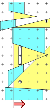
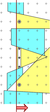
(a) (b)

Figure 3: (a) Just before and (b) just after the sweepline crosses the right edge of a trapezoid and its neighboring gaps are merged. Leftmost pixels in each gap, if any, are circled.

We store the traps and gaps in two data structures: a balanced binary search tree and a priority queue. The binary tree stores the traps and gaps in sorted order from top to bottom along $\ell$. For the priority queue, the priority of a trap is the $x$-coordinate of its right edge, and the priority of a gap is the $x$-coordinate of the leftmost pixel(s) inside the gap, or $\infty$ if the gap contains no pixels. Since the sweepline clearly crosses at most $t$ trapezoids, the cost of inserting or deleting a trap or gap from the sweep structures is $O(\log t)$. Note that this is bounded by both $O(\log p)$ and $O(\log n)$.

To find the leftmost pixel inside a gap, we use the following two-dimensional integer programming result of Kanamaru et al. [31]; see also [32, 19]. For related results on enumerating integer points in convex polygons, see [34, 35, 26, 27].

Lemma 5.1 (Kanamaru et al. [31])

Given a convex $m$-gon $\Pi$, we can find the lowest leftmost integer point in $\Pi$, or determine that $\Pi$ contains no integer points, in time $O(m+\log\delta)$, where $\delta$ is the length of the shortest edge of the axis-aligned bounding box of $\Pi$.

Corollary 5.2

We can find a leftmost pixel in any gap, or determine that there is no such pixel, in $O(\log p)$ time.

We do not require that the sweepline structures always contain every trapezoid in ${Vis(\Delta\mid\nobreak P)}$ that intersects $\ell$. Instead we maintain the following weaker invariant: whenever $\ell$ reaches a pixel $\pi$, the trapezoid $\tau_{\pi}\in{Vis(\Delta\mid\nobreak P)}$ containing $\pi$ must be stored in the sweepline structures. We initialize the sweep structure with a single gap that contains the entire pixel grid.

When the sweepline $\ell$ reaches the right edge of a trap $\tau$, we delete it from the sweep structure. We also delete the gaps immediately above and below $\tau$ and insert the new larger gap. Manipulating the sweep structure requires $O(\log t)$ time, and finding a leftmost pixel in the new gap requires $O(\log p)$ time, so the total time required to kill a single trap is $O(\log p)$.

When $\ell$ reaches a leftmost pixel $\pi$ in a gap $\gamma$, we perform a trapezoid query to find the trap $\tau_{\pi}\in{Vis(\Delta\mid\nobreak P)}$ containing $\pi$. We then delete $\gamma$ from the sweep structure, insert $\tau_{\pi}$, and insert the two smaller gaps $\gamma^{+}$ and $\gamma^{-}$ immediately above and below $\tau_{\pi}$. The new trap $\tau_{\pi}$ may not contain all the leftmost pixels in $\gamma$; any omitted pixels will now be a leftmost pixel in either $\gamma^{+}$ or $\gamma^{-}$. If some new gap contains a leftmost pixel of $\gamma$, it will be (recursively) filled before the sweepline moves again. (We can avoid creating such “transient” gaps by storing the highest and lowest leftmost pixels in each gap $\gamma$, at an additional cost of $O(1)$ time when $\gamma$ is created, but this improves the running time of our algorithm by at most a constant factor.) For each new trap inserted, our algorithm spends $O(\log p)$ time and creates at most two new gaps.

Every gap except the initial one is created when a trap is inserted or deleted. We can charge at most three gaps to each trap: the gaps immediately above and below when the trap is inserted, and the gap left behind when the trap is deleted. The total number of gaps created over the entire algorithm is therefore at most $3t+1$. It follows that the total time spent finding leftmost pixels is $O(t\log p)$, and the total time spent manipulating the sweep structures is $O(t\log t)$. All the remaining time is spent on trapezoid queries, as in our earlier algorithms.

Theorem 5.3

Let $\Delta$ be a set of $n$ disjoint triangles in $\mathrm{I\!R}^{3}$, and let $P$ be a regular lattice of $p$ points in the $xy$-plane. We can construct ${Vis(\Delta\mid\nobreak P)}$ in time $O(n^{1+\varepsilon}+t^{2/3}n^{2/3+\varepsilon}+t\log p)$, where $t$ is the number of trapezoids in ${Vis(\Delta\mid\nobreak P)}$.

Note that this time bound is sublinear in $p$ unless $t=\Omega(p/\log p)$. Moreover, the $O(t\log p)$ term is dominated by other terms unless either $t$ is nearly quadratic in $n$ or $p=2^{\Omega(n^{c})}$ for some positive constant $c$.

6 Discussion and Open Problems

One interesting special case of hidden-surface removal is the so-called window rendering problem, where the objects are axis-aligned horizontal rectangles. A simple modification of our algorithm solves this problem in time $O(n\log^{2}n+t\log n+p)$ which compares favorably with the best analytic solutions [8, 22]. If the pixels form a regular grid, we can improve the running time to $O(n\log^{2}n+t\log n)$ using the sweepline approach. (Note that this time bound does not depend at all on the number of pixels!) Similar improvements can be made for $c$-oriented polyhedra [7]. It seems likely that our techniques can also be extended to other special cases of hidden surface removal with faster analytic solutions, such a polyhedral terrains [43] and objects whose union has small complexity [33, 25].

Perhaps the most interesting open question is whether sampled visibility maps, or some other similar image decomposition, can be constructed efficiently in practice. As we mentioned in the introduction, ray-shooting queries are already answered in practice by walking through a spatial decomposition defined by the input objects. The same spatial decomposition can also be used to answer ray-dragging queries [40] and trapezoidal beam queries. Since curved models are often polygonalized (and complex polyhedral models are often simplified) so that each polygonal facet covers only a few pixels, a practical implementation may require the sampled visibility map to be redefined in terms of higher-level objects, such as convex polyhedra or algebraic surface patches, instead of triangles.

A practical implementation of our ideas would have other interesting applications. By changing the order in which our algorithm processes pixels, we can make it suitable for progressive rendering, where the quality of the image improves smoothly over time as finer and finer details are computed, or foveated rendering, where fine details are more important in certain areas of the image than others. Another possible application is occlusion culling [12, 13, 30, 36, 47]. By sampling the visibility map at a small number of random points, we can quickly establish a set of simple occluders that can be used for conservative visibility tests. The occlusion tests themselves would be slightly simpler than in earlier approaches: A triangle is invisible if its projection is contained in some trapezoid.

Sampled visibility maps exploit spatial coherence well in a global sense; the number of regions is never much larger than the size of the visibility map. In a more local sense, however, there is clearly room for improvement. Consider an image that contains mostly empty space, except for a large number of small triangles near the boundary. The sampled visibility map consists of several tall thin trapezoids, but a better decomposition would have a single region covering most of the image. It would be interesting to develop decompositions with better local behavior—perhaps where the expected size of the component containing a random pixel is maximized, or where the size of a component is tied to the local feature size [44] of the visibility map near that component—but with the same global properties as sampled visibility maps.

Acknowledgment.

I thank Pavan Desikan and Sariel Har-Peled for suggesting the sweep-line approach described in Section 5 and pointing out several relevant references [26, 27, 34].

References

- [1] P. K. Agarwal and J. Erickson. Geometric range searching and its relatives. Advances in Discrete and Computational Geometry, pp. 1–56. Contemporary Mathematics 223, AMS Press, 1999.
- [2] P. K. Agarwal and J. Matoušek. Ray shooting and parametric search. SIAM J. Comput. 22(4):794–806, 1993.
- [3] P. K. Agarwal and M. Sharir. Applications of a new space-partitioning technique. Discrete Comput. Geom. 9:11–38, 1993.
- [4] B. Aronov and S. Fortune. Average-case ray shooting and minimum weight triangulations. Proc. 13th Annu. ACM Sympos. Comput. Geom., pp. 203–211. 1997.
- [5] J. L. Bentley. Multidimensional divide-and-conquer. Commun. ACM 23(4):214–229, 1980.
- [6] M. de Berg, D. Halperin, M. Overmars, J. Snoeyink, and M. van Kreveld. Efficient ray shooting and hidden surface removal. Algorithmica 12(1):30–53, 1994.
- [7] M. de Berg and M. Overmars. Hidden surface removal for -oriented polyhedra. Comput. Geom. Theory Appl. 1(5):247–268, 1992.
- [8] M. Bern. Hidden surface removal for rectangles. J. Comput. Syst. Sci. 40:49–69, 1990.
- [9] E. E. Catmull. A Subdivision Algorithm for Computer Display of Curved Surfaces. Ph.D. Thesis, Univ. Utah, Salt Lake City, UT, December 1974. Tech. Rep. UTEC-CSc-74-133.
- [10] B. Chazelle and L. J. Guibas. Fractional cascading: I. A data structuring technique. Algorithmica 1(3):133–162, 1986.
- [11] B. Chazelle and L. J. Guibas. Fractional cascading: II. Applications. Algorithmica 1:163–191, 1986.
- [12] D. Cohen-Or, G. Fibich, D. Halperin, and E. Zadicario. Conservative visibility and strong occlusion for viewspace partitioning of densely occluded scenes. Comput. Graph. Forum 17:243–253, 1998.
- [13] S. Coorg and S. Teller. Real-time occlusion culling for models with large occluders. Proc. 1997 Sympos. Interactive 3D Graphics, pp. 83–90. 1997.
- [14] P. Desikan and S. Har-Peled. Personal communication, 1999.
- [15] F. Dévai. Quadratic bounds for hidden line elimination. Proc. 2nd Annu. ACM Sympos. Comput. Geom., pp. 269–275. 1986.
- [16] D. Dobkin, J. Hershberger, D. Kirkpatrick, and S. Suri. Implicitly searching convolutions and computing depth of collision. Proc. 1st Annu. SIGAL Internat. Sympos. Algorithms, pp. 165–180. Lecture Notes Comput. Sci. 450, Springer-Verlag, 1990.
- [17] S. E. Dorward. A survey of object-space hidden surface removal. Internat. J. Comput. Geom. Appl. 4:325–362, 1994.
- [18] J. Erickson. New lower bounds for Hopcroft’s problem. Discrete Comput. Geom. 16:389–418, 1996.
- [19] S. D. Feit. A fast algorithm for the two-variable integer programming problem. J. Assoc. Comput. Mach. 31(1):99–113, 1984.
- [20] J. D. Foley, A. van Dam, S. K. Feiner, and J. F. Hughes. Computer Graphics: Principles and Practice. Addison-Wesley, Reading, MA, 1990. second edition.
- [21] A. S. Glassner. Space subdivision for fast ray tracing. IEEE Comput. Graph. Appl. 4(10):15–22, Oct. 1984.
- [22] M. T. Goodrich, M. J. Atallah, and M. H. Overmars. Output-sensitive methods for rectilinear hidden surface removal. Inform. Comput. 107:1–24, 1993.
- [23] N. Greene, M. Kass, and G. Miller. Hierachical Z-buffer visibility. Proc. SIGGRAPH ’93, pp. 273–278, 1993.
- [24] N. Greene. Heirarchical polygon tiling with coverage masks. Proc. SIGGRAPH ’96, pp. 65–74. 1996.
- [25] D. Halperin and M. H. Overmars. Spheres, molecules, and hidden surface removal. Proc. 10th Annu. ACM Sympos. Comput. Geom., pp. 113–122. 1994.
- [26] S. Har-Peled. An output sensitive algorithm for discrete convex hulls. Comput. Geom. Theory Appl. 10:125–138, 1998.
- [27] W. Harvey. Computing two-dimensional integer hulls. SIAM J. Comput. 28(6):2285–2299, 1999.
- [28] P. S. Heckbert and P. Hanrahan. Beam tracing polygonal objects. Comput. Graph. 18(3):119–127, 1984. Proc. SIGGRAPH ’84.
- [29] J. Hershberger and S. Suri. A pedestrian approach to ray shooting: Shoot a ray, take a walk. J. Algorithms 18:403–431, 1995.
- [30] T. Hudson, D. Manocha, J. Cohen, M. Lin, K. Hoff, and H. Zhang. Accelerated occlusion culling using shadow frustra. Proc. 13th Annu. ACM Sympos. Comput. Geom., pp. 1–10. 1997.
- [31] N. Kanamaru, T. Nishizeki, and T. Asano. Efficient enumeration of grid points in a polygon and its application to integer programming. Internat. J. Comput. Geom. Appl. 4:69–85, 1994.
- [32] R. Kannan. A polynomial algorithm for the two-variable integer programming problem. J. Assoc. Comput. Mach. 27(1):118–122, 1980.
- [33] M. J. Katz, M. H. Overmars, and M. Sharir. Efficient hidden surface removal for objects with small union size. Comput. Geom. Theory Appl. 2:223–234, 1992.
- [34] H. S. Lee and R. C. Chang. Approximating vertices of a convex polygon with grid points in the polygon. Proc. 3rd Annu. Internat. Sympos. Algorithms Comput., pp. 269–278. Lecture Notes Comput. Sci. 650, Springer-Verlag, 1992.
- [35] H. S. Lee and R. C. Chang. Regular enumeration of grid points in a convex polygon. Internat. J. Comput. Geom. Appl. 3:305–322, 1993.
- [36] D. Luebke and C. Georges. Portals and mirrors: Simple, fast evaluation of potentially v isible sets. Proc. ACM Interactive 3D Graphics Conf., pp. 105–106. 1995.
- [37] J. Matoušek. Range searching with efficient hierarchical cuttings. Discrete Comput. Geom. 10(2):157–182, 1993.
- [38] M. McKenna. Worst-case optimal hidden-surface removal. ACM Trans. Graph. 6:19–28, 1987.
- [39] K. Mehlhorn and S. Näher. Dynamic fractional cascading. Algorithmica 5:215–241, 1990.
- [40] T. M. Murali. Efficient Hidden-Surface Removal in Theory and in Practice. Ph.D. Thesis, Brown Univ., Providence, RI, June 1998. http://robotics.stanford.edu/~murali/papers/thesis/.
- [41] M. H. Overmars and M. Sharir. An improved technique for output-sensitive hidden surface removal. Algorithmica 11(5):469–484, 1994.
- [42] M. S. Paterson and F. F. Yao. Efficient binary space partitions for hidden-surface removal and solid modeling. Discrete Comput. Geom. 5:485–503, 1990.
- [43] J. H. Reif and S. Sen. An efficient output-sensitive hidden-surface removal algorithms and its parallelization. Proc. 4th Annu. ACM Sympos. Comput. Geom., pp. 193–200. 1988.
- [44] J. Ruppert. A Delaunay refinement algorithm for quality 2-dimensional mesh generation. J. Algorithms 18(3):548–585, 1995.
- [45] F. Sillion and C. Puech. Radiosity and Global Illumination. Morgan Kauffmann, 1994.
- [46] I. E. Sutherland, R. F. Sproull, and R. A. Schumacker. A characterization of ten hidden-surface algorithms. ACM Comput. Surv. 6(1):1–55, 1974.
- [47] S. J. Teller. Visibility Computations in Densely Occluded Polyhedral Environments. Ph.D. thesis, Comput. Sci. Div., Univ. California, Berkeley, 1992.
- [48] S. Teller and J. Alex. Frustum casting for progressive, interactive rendering. Tech. Rep. MIT LCS TR-740, MIT Lab. Comput. Sci., January 1998.
- [49] J. Warnock. A hidden-surface algorithm for computer generated half-tone pictures. Tech. Rep. 4-15, NTIS AD-733 671, Comput. Sci. Dept., Univ. Utah, 1969.
- [50] K. Weiler and P. Atherton. Hidden surface removal using polygon area sorting. Comput. Graph. 11(2):214–222, 1977. Proc. SIGGRAPH ’77.