Processor Verification Using Efficient Reductions
of the Logic of Uninterpreted Functions
to Propositional Logic.

Abstract

The logic of equality with uninterpreted functions (EUF) provides a means of abstracting the manipulation of data by a processor when verifying the correctness of its control logic. By reducing formulas in this logic to propositional formulas, we can apply Boolean methods such as Ordered Binary Decision Diagrams (BDDs) and Boolean satisfiability checkers to perform the verification.

We can exploit characteristics of the formulas describing the verification conditions to greatly simplify the propositional formulas generated. We identify a class of terms we call “p-terms” for which equality comparisons can only be used in monotonically positive formulas. By applying suitable abstractions to the hardware model, we can express the functionality of data values and instruction addresses flowing through an instruction pipeline with p-terms. A decision procedure can exploit the restricted uses of p-terms by considering only “maximally diverse” interpretations of the associated function symbols, where every function application yields a different value except when constrained by functional consistency.

We present two methods to translate formulas in EUF into propositional logic. The first interprets the formula over a domain of fixed-length bit vectors and uses vectors of propositional variables to encode domain variables. The second generates formulas encoding the conditions under which pairs of terms have equal valuations, introducing propositional variables to encode the equality relations between pairs of terms. Both of these approaches can exploit maximal diversity to greatly reduce the number of propositional variables that need to be introduced and to reduce the overall formula sizes.

We present experimental results demonstrating the efficiency of this approach when verifying pipelined processors using the method proposed by Burch and Dill. Exploiting positive equality allows us to overcome the exponential blow-up experienced previously [VB98] when verifying microprocessors with load, store, and branch instructions.

Keywords: Formal verification, Processor verification, Uninterpreted functions, Decision procedures

1 Introduction

For automatically reasoning about pipelined processors, Burch and Dill demonstrated the value of using propositional logic, extended with uninterpreted functions, uninterpreted predicates, and the testing of equality [BD94]. Their approach involves abstracting the data path as a collection of registers and memories storing data, units such as ALUs operating on the data, and various connections and multiplexors providing methods for data to be transferred and selected. The initial state of each register is represented by a domain variable indicating an arbitrary data value. The operation of units that transform data is abstracted as blocks computing functions with no specified properties other than functional consistency, i.e., that applications of a function to equal arguments yield equal results: $x=y\Rightarrow f(x)=f(y)$. The state of a register at any point in the computation can be represented by a symbolic term, an expression consisting of a combination of domain variables, function and predicate applications, and Boolean operations. Verifying that a pipelined processor has behavior matching that of an unpipelined instruction set reference model can be performed by constructing a formula in this logic that compares for equality the terms describing the results produced by the two models and then proving the validity of this formula.

In their 1994 paper, Burch and Dill also described the implementation of a decision procedure for this logic based on theorem proving search methods. Their procedure builds on ones originally described by Shostak [Sho79] and by Nelson and Oppen [NO80], using combinatorial search coupled with algorithms for maintaining a partitioning of the terms into equivalence classes based on the equalities that hold at a given step of the search. More details of their decision procedure are given in [JDB95].

Burch and Dill’s work has generated considerable interest in the use of uninterpreted functions to abstract data operations in processor verification. A common theme has been to adopt Boolean methods, either to allow integration of uninterpreted functions into symbolic model checkers [DPR98, BBCZ98], or to allow the use of Binary Decision Diagrams (BDDs) [Bry86] in the decision procedure [HKGB97, GSZAS98, VB98]. Boolean methods allow a more direct modeling of the control logic of hardware designs and thus can be applied to actual processor designs rather than highly abstracted models. In addition to BDD-based decision procedures, Boolean methods could use some of the recently developed satisfiability procedures for propositional logic. In principle, Boolean methods could outperform decision procedures based on theorem proving search methods, especially when verifying processors with more complex control logic, e.g., due to superscalar or out-of-order operation.

Boolean methods can be used to decide the validity of a formula containing terms and uninterpreted functions by interpreting the formula over a domain of fixed-length bit vectors. Such an approach exploits the property that a given formula contains a limited number of function applications and therefore can be proved to be universally valid by considering its interpretation over a sufficiently large, but finite domain [Ack54]. If a formula contains a total of $m$ function applications, then the set of all bit vectors of length $k$ forms an adequate domain for $k\geq\log_{2}m$. The formula to be verified can be translated into one in propositional logic, using vectors of propositional variables to encode the possible values generated by function applications [HKGB97]. Our implementation of such an approach [VB98] as part of a BDD-based symbolic simulation system was successful at verifying simple pipelined data paths. We found, however, that the computational resources grew exponentially as we increased the pipeline depth. Modeling the interactions between successive instructions flowing through the pipeline, as well as the functional consistency of the ALU results, precludes having an ordering of the variables encoding term values that yields compact BDDs. Similarly, we found that extending the data path to a complete processor by adding either load and store instructions or instruction fetch logic supporting jumps and conditional branches led to impossible BDD variable ordering requirements.

Goel et al.  [GSZAS98] present an alternate approach to using BDDs to decide the validity of formulas in the logic of equality with uninterpreted functions. In their formulation they introduce a propositional variable $e_{i,j}$ for each pair of function application terms $T_{i}$ and $T_{j}$, expressing the conditions under which the two terms are equal. They add constraints expressing both functional consistency and the transitivity of equality among the terms. Their experimental results were also somewhat disappointing. For all previous methods of reducing EUF to propositional logic, Boolean methods have not lived up to their promise of outperforming ones based on theorem proving search.

In this paper, we show that the characteristics of the formulas generated when modeling processor pipelines can be exploited to greatly reduce the number of propositional variables that are introduced when translating the formula into propositional logic. We distinguish a class of terms we call p-terms for which equality comparisons can be used only in monotonically positive formulas. Such formulas are suitable for describing the top-level correctness condition, but not for modeling any control decisions in the hardware. By applying suitable abstractions to the hardware model, we can express the functionality of data values and instruction addresses with p-terms.

A decision procedure can exploit the restricted uses of p-terms by considering only “maximally diverse” interpretations of the associated “p-function” symbols, where every function application yields a different value except when constrained by functional consistency. We present a method of transforming a formula containing function applications into one containing only domain variables that differs from the commonly-used method described by Ackermann [Ack54]. Our method allows a translation into propositional logic that uses vectors with fixed bit patterns rather than propositional variables to encode domain variables introduced while eliminating p-function applications. This reduction in propositional variables greatly simplifies the BDDs generated when checking tautology, often avoiding the exponential blow-up experienced by other procedures. Alternatively, we can use a encoding scheme similar to Goel et al.  [GSZAS98], but with many of the $e_{i,j}$ values set to ${\bf false}$ rather than to Boolean variables.

Others have recognized the value of restricting the testing of equality when modeling the flow of data in pipelines. Berezin et al.  [BBCZ98] generate a model of an execution unit suitable for symbolic model checking in which the data values and operations are kept abstract. In our terminology, their functional terms are all p-terms. They use fixed bit patterns to represent the initial states of registers, much as we replace p-term domain variables by fixed bit patterns. To model the outcome of each program operation, they generate an entry in a “reference file” and refer to the result by a pointer to this file. These pointers are similar to the bit patterns we generate to denote the p-function application outcomes. This paper provides an alternate, and somewhat more general view of the efficiency gains allowed by p-terms.

Damm et al.  consider an even more restricted logic such that in the terms describing the computed result, no function symbol is applied to a term that already contains the same symbol. As a consequence, they can guarantee that an equality between two terms holds universally if it holds holds over the domain $\{0,1\}$ and with function symbols having four possible interpretations: constant functions 0 or 1, and projection functions selecting the first or second argument. They can therefore argue that verifying an execution unit in which the data path width is reduced to a single bit and in which the functional units implement only four functions suffices to prove its correctness for all possible widths and functionalities. Their work imposes far greater restrictions than we place on p-terms, but it allows them to bound the domain that must be considered to determine universal validity independently from the formula size.

In comparison to both of these other efforts, we maintain the full generality of the unrestricted terms of Burch and Dill while exploiting the efficiency gains possible with p-terms. In our processor model, we can abstract register identifiers as unrestricted terms, while modeling program data and instruction data as p-terms. As a result, our verifications cover designs with arbitrarily many registers. In contrast, both [BBCZ98] and [DPR98] used bit encodings of register identifiers and were unable to scale their verifications to a realistic number of registers.

In a recent paper, Pnueli, et al. [PRSS99] also propose a method to exploit the polarity of the equations in a formula containing uninterpreted functions with equality. They describe an algorithm to generate a small domain for each domain variable such that the universal validity of the formula can be determined by considering only interpretations in which the variables range over their restricted domains. A key difference of their work is that they examine the equation structure after replacing all function application terms with domain variables and introducing functional consistency constraints as described by Ackermann [Ack54]. These consistency constraints typically contain large numbers of equations—far more than occur in the original formula—that mask the original p-term structure. As an example, comparing the top and bottom parts of Figure 6 illustrates the large number of equations that may be generated when applying Ackermann’s method. By contrast, our method is based on the original formula structure. In addition, we use a new method of replacing function application terms with domain variables. Our scheme allows us to exploit maximal diversity by assigning fixed values to the domain variables generated while expanding p-function application terms. Quite possibly, a variant of their method could be used to generate a small domain for each of the other variables in the formula.

The remainder of the paper is organized as follows. We define the syntax and semantics of our logic by extending that of Burch and Dill’s. We describe a simple procedure for automatically converting a formula from Burch and Dill’s logic to ours. We prove our central result concerning the need to consider only maximally diverse interpretations when deciding the validity of formulas in our logic. As a first step in transforming our logic into propositional logic, we describe a new method of eliminating function application terms in a formula. Building on this, we describe two methods of translating formulas into propositional logic and show how these methods can exploit the properties of p-terms. We discuss the abstractions required to model processor pipelines in our logic. Finally, we present experimental results showing our ability to verify a simple, but complete pipelined processor. More complete details on an implementation that has successfully verified several superscalar processor designs are presented in [VB99].

2 Logic of Equality with Uninterpreted Functions (EUF)

term $$\mathrel{::=} \mbox{{\rm{\it ITE}}}(\mbox{{\rm{\it formula}}},\mbox{{\rm{\it term}}},\mbox{{\rm{\it term}}})$$

$$|\;\mbox{{\rm{\it function-symbol}}}(\mbox{{\rm{\it term}}},\ldots,\mbox{{\rm{\it term}}})$$

formula $$\mathrel{::=} {\bf true}\mathbin{|}{\bf false}\mathbin{|}\neg\mbox{{\rm{\it formula}}}$$

$$|\;(\mbox{{\rm{\it formula}}}\land\mbox{{\rm{\it formula}}})\mathbin{|}(\mbox{{\rm{\it formula}}}\lor\mbox{{\rm{\it formula}}})$$

$$|\;(\mbox{{\rm{\it term}}}\!=\!\mbox{{\rm{\it term}}})$$

$$|\;\mbox{{\rm{\it predicate-symbol}}}(\mbox{{\rm{\it term}}},\ldots,\mbox{{\rm{\it term}}})$$

Figure 1: Syntax Rules for the Logic of Equality with Uninterpreted Functions (EUF)

The logic of Equality with Uninterpreted Functions (EUF) presented by Burch and Dill [BD94] can be expressed by the syntax given in Figure 1. In this logic, formulas have truth values while terms have values from some arbitrary domain. Terms are formed by application of uninterpreted function symbols and by applications of the ITE (for “if-then-else”) operator. The ITE operator chooses between two terms based on a Boolean control value, i.e., $\mbox{{\rm{\it ITE}}}({\bf true},x_{1},x_{2})$ yields $x_{1}$ while $\mbox{{\rm{\it ITE}}}({\bf false},x_{1},x_{2})$ yields $x_{2}$. Formulas are formed by comparing two terms with equality, by applying an uninterpreted predicate symbol to a list of terms, and by combining formulas using Boolean connectives. A formula expressing equality between two terms is called an equation. We use expression to refer to either a term or a formula.

Every function symbol $f$ has an associated order, denoted ${\it ord}(f)$, indicating the number of terms it takes as arguments. Function symbols of order zero are referred to as domain variables. We use the shortened form $v$ rather than $v()$ to denote an instance of a domain variable. Similarly, every predicate $p$ has an associated order ${\it ord}(p)$. Predicates of order zero are referred to as propositional variables, and can be written $a$ rather than $a()$.

Form $E$	Valuation $I[E]$
true	true
false	false
$\neg F$	$\neg I[F]$
$F_{1}\land F_{2}$	$I[F_{1}]\land I[F_{2}]$
$p(T_{1},\ldots,T_{k})$	$I(p)(I[T_{1}],\ldots,I[T_{k}])$
$T_{1}\!=\!T_{2}$	$I[T_{1}]\!=\!I[T_{2}]$
$\mbox{{\rm{\it ITE}}}(F,T_{1},T_{2})$	$\mbox{{\rm{\it ITE}}}(I[F],I[T_{1}],I[T_{2}])$
$f(T_{1},\ldots,T_{k})$	$I(f)(I[T_{1}],\ldots,I[T_{k}])$

Table 1: Evaluation of EUF Formulas and Terms

The truth of a formula is defined relative to a nonempty domain ${\cal D}$ of values and an interpretation $I$ of the function and predicate symbols. Interpretation $I$ assigns to each function symbol of order $k$ a function from ${\cal D}^{k}$ to ${\cal D}$, and to each predicate symbol of order $k$ a function from ${\cal D}^{k}$ to $\{{\bf true},{\bf false}\}$. For the special case of order 0 symbols, i.e., domain (respectively, propositional) variables, the interpretation assigns an element of ${\cal D}$ (resp., $\{{\bf true},{\bf false}\}$.) Given an interpretation $I$ of the function and predicate symbols and an expression $E$, we can define the valuation of $E$ under $I$, denoted $I[E]$, according to its syntactic structure. The valuation is defined recursively, as shown in Table 1. $I[E]$ will be an element of the domain when $E$ is a term, and a truth value when $E$ is a formula.

A formula $F$ is said to be true under interpretation $I$ when $I[F]={\bf true}$. It is said to be valid over domain ${\cal D}$ when it is true over domain ${\cal D}$ for all interpretations of the symbols in $F$. $F$ is said to be universally valid when it is valid over all domains. A basic property of validity is that a given formula is valid over a domain ${\cal D}$ iff it is valid over all domains having the same cardinality as ${\cal D}$. This follows from the fact that a given formula has the same truth value in any two isomorphic interpretations of the symbols in the formula. Another property of the logic, which can be readily shown, is that if $F$ is valid over a suitably large domain, then it is universally valid [Ack54]. In particular, it suffices to have a domain as large as the number of syntactically distinct function application terms occurring in $F$. We are interested in decision procedures that determine whether or not a formula is universally valid; we will show how to do this by dynamically constructing a sufficiently large domain as the formula is being analyzed.

3 Positive Equality with Uninterpreted Functions (PEUF)

g-term $$\mathrel{::=} \mbox{{\rm{\it ITE}}}(\mbox{{\rm{\it g-formula}}},\mbox{{\rm{\it g-term}}},\mbox{{\rm{\it g-term}}})$$

$$|\;\mbox{{\rm{\it g-function-symbol}}}(\mbox{{\rm{\it p-term}}},\ldots,\mbox{{\rm{\it p-term}}})$$

p-term $$\mathrel{::=}$$ g-term

$$|\;\mbox{{\rm{\it ITE}}}(\mbox{{\rm{\it g-formula}}},\mbox{{\rm{\it p-term}}},\mbox{{\rm{\it p-term}}})$$

$$|\;\mbox{{\rm{\it p-function-symbol}}}(\mbox{{\rm{\it p-term}}},\ldots,\mbox{{\rm{\it p-term}}})$$

g-formula $$\mathrel{::=} {\bf true}\mathbin{|}{\bf false}\mathbin{|}\neg\mbox{{\rm{\it g-formula}}}$$

$$|\;(\mbox{{\rm{\it g-formula}}}\land\mbox{{\rm{\it g-formula}}})\mathbin{|}(\mbox{{\rm{\it g-formula}}}\lor\mbox{{\rm{\it g-formula}}})$$

$$|\;(\mbox{{\rm{\it g-term}}}\!=\!\mbox{{\rm{\it g-term}}})$$

$$|\;\mbox{{\rm{\it predicate-symbol}}}(\mbox{{\rm{\it p-term}}},\ldots,\mbox{{\rm{\it p-term}}})$$

p-formula $$\mathrel{::=}$$ g-formula

$$|\;(\mbox{{\rm{\it p-formula}}}\land\mbox{{\rm{\it p-formula}}})\mathbin{|}(\mbox{{\rm{\it p-formula}}}\lor\mbox{{\rm{\it p-formula}}})$$

$$|\;(\mbox{{\rm{\it p-term}}}\!=\!\mbox{{\rm{\it p-term}}})$$

Figure 2: Syntax Rules for the Logic of Positive Equality with Uninterpreted Functions (PEUF)

We can improve the efficiency of validity checking by treating positive and negative equations differently when reducing EUF to propositional logic. Informally, an equation is positive if it does not appear negated in a formula. In particular, a positive equation cannot appear as the formula that controls the value of an ITE term; such formulas are considered to appear both positively and negatively.

3.1 Syntax

PEUF is an extended logic based on EUF; its syntax is shown in Figure 2. The main idea is that there are two disjoint classes of function symbols, called p-function symbols and g-function symbols, and two classes of terms.

General terms, or g-terms, correspond to terms in EUF. Syntactically, a g-term is a g-function application or an ITE term in which the two result terms are hereditarily built from g-function applications and ITEs.

The new class of terms is called positive terms, or p-terms. P-terms may not appear in negated equations, i.e., equations within the scope of a logical negation. Since p-terms can contain p-function symbols, the syntax is restricted in a way that prevents p-terms from appearing in negative equations. When two p-terms are compared for equality, the result is a special, restricted kind of formula called a p-formula.

Note that our syntax allows any g-term to be “promoted” to a p-term. Throughout the syntax definition, we require function and predicate symbols to take p-terms as arguments. However, since g-terms can be promoted, the requirement to use p-terms as arguments does not restrict the use of g-function symbols or g-terms. In essence, g-function symbols may be used as freely in our logic as in EUF, but the p-function symbols are restricted. To maintain the restriction on p-function symbols, the syntax does not permit a p-term to be promoted to a g-term.

A g-formula is a Boolean combination of equations on g-terms and applications of predicate symbols. G-formulas in our logic serve as Boolean control expressions in ITE terms. A g-formula can contain negation, and ITE implicitly negates its Boolean control, so only g-terms are allowed in equations in g-formulas.

Finally, the syntactic class p-formula is the class for which we develop validity checking methods. p-formulas are built up using only the monotonically positive Boolean operations $\land$ and $\lor$. P-formulas may not be placed under a negation sign and cannot be used as the control for an ITE operation. As described in later sections, our validity checking methods will take advantage of the assumption that in p-formulas, the p-terms cannot appear in negative equations.

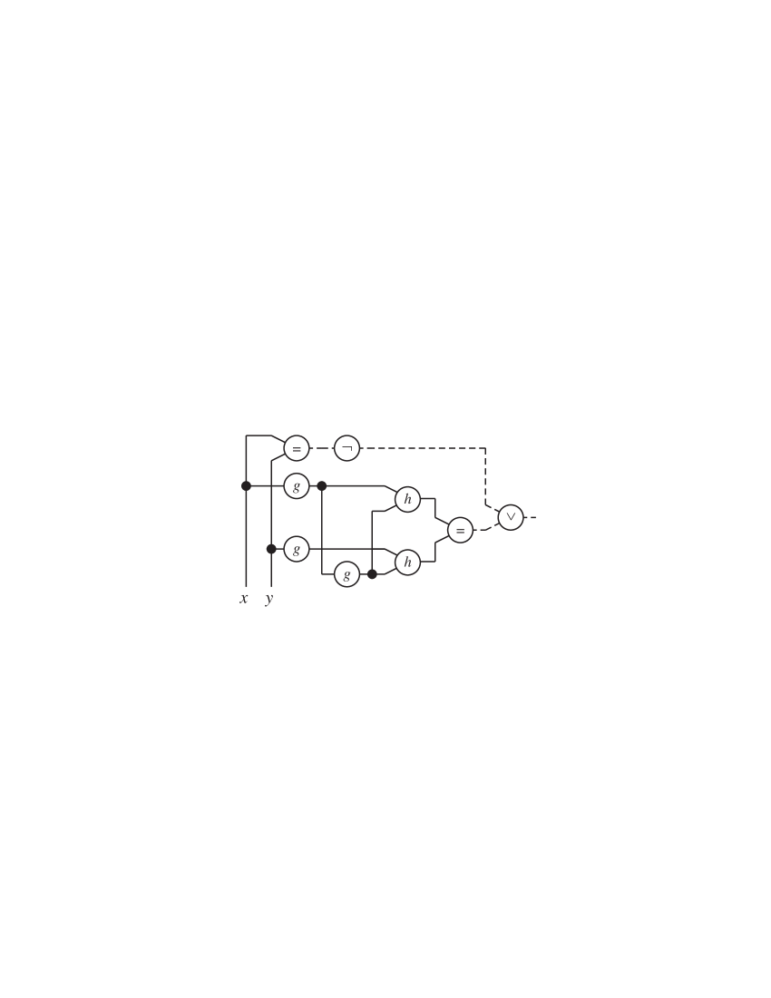
Figure 3: Schematic Representation of $F_{\rm eg}$. Domain values are shown as solid lines, while truth values are shown as dashed lines.

As a running example for this paper, we consider the formula $x\!=\!y\Rightarrow h(g(x),g(g(x)))\!=\!h(g(y),g(g(x)))$, which would be transformed into a p-formula $F_{\rm eg}$ by eliminating the implication:

$$F_{\rm eg} = \neg(x\!=\!y)\;\;\lor\;\;h(g(x),g(g(x)))\!=\!h(g(y),g(g(x)))$$ (1)

Domain variables $x$ and $y$ must be g-function symbols so that we can consider the equation $x\!=\!y$ to be a g-formula, and hence it can be negated to give g-formula $\neg(x\!=\!y)$. We can promote the g-terms $x$ and $y$ to p-terms, and we can consider function symbols $g$ and $h$ to be p-function symbols, giving p-terms $g(x)$, $g(y)$, $g(g(x))$, $h(g(x),g(g(x)))$, and $h(g(y),g(g(x)))$. Thus, the equation $h(g(x),g(g(x)))\!=\!h(g(y),g(g(x)))$ is a p-formula. We form the disjunction of this p-formula with the p-formula obtained by promoting $\neg(x\!=\!y)$ giving p-formula $F_{\rm eg}$.

Figure 3 shows a schematic representation of $F_{\rm eg}$, using drawing conventions similar to those found in hardware designs. That is, we view domain variables as inputs (shown along bottom) to a network of operators. Domain values are denoted with solid lines, while truth values are denoted with dashed lines. The top-level formula then becomes the network output, shown on the right. The operators in the network are shared whenever possible. This representation is isomorphic to the traditional directed acyclic graph (DAG) representation of an expression, with maximal sharing of common subexpressions.

3.2 Extracting PEUF from EUF

Observe that PEUF does not extend the expressive power of EUF—we could translate any PEUF expression into EUF by considering both the p-terms and g-terms to be terms and both the p-formulas and g-formulas to be formulas. Instead, the benefit of PEUF is that by distinguishing some portion of a formula as satisfying a restricted set of properties, we can radically reduce the number of different interpretations we must consider when proving that a p-formula is universally valid.

In fact, we can automatically extract the PEUF syntax from an EUF formula by the following process, and hence our decision procedure can be viewed as one that automatically exploits the polarity structure of equations in an arbitrary EUF formula $F_{\mbox{top}}$. The main task is to classify the function symbols as either p-function or g-function symbols.

We assume our EUF formula $F_{\mbox{top}}$ is in negation-normal form, meaning that the negation operation $\neg$ is applied only to equations and predicate applications. We can convert an arbitrary formula into negation-normal form by applying the following syntactic transformations:

$$\neg{\bf true} \rightarrow {\bf false}$$

$$\neg{\bf false} \rightarrow {\bf true}$$

$$\neg\neg F \rightarrow F$$

$$\neg(F_{1}\land F_{2}) \rightarrow \neg F_{1}\lor\neg F_{2}$$

$$\neg(F_{1}\lor F_{2}) \rightarrow \neg F_{1}\land\neg F_{2}$$

To formalize the relationship between EUF expressions and PEUF expressions, we introduce a tree representation of EUF expressions. The rules for the tree representation are as follows:

1. If $E$ is an EUF expression having no proper subexpressions (${\bf true}$, ${\bf false}$, a domain variable, or a propositional variable), then $E$ is represented by a tree consisting of a single node labelled with $E$.

2. If $E$ is an EUF expression having $n$ proper subexpressions, then $E$ is represented by a tree whose root node is labelled with the main operator ($=$, ITE, $\land$, $\lor$, $\neg$, predicate symbol, function symbol). Attached to the root node are $n$ subtrees, where the $i$th subtree represents the $i$th proper subexpression.

We define a parsing of an EUF expression as a PEUF expression. Let $t$ be a tree representing an EUF expression $E$. A parsing of $E$ as a PEUF expression is a function that assigns to each node of $t$ a set of syntax classes in the formal syntax of PEUF, such that the syntax rules of PEUF (Figure 2) are satisfied. Note that this definition allows multiple syntax classes to be assigned to a given tree node. This multiplicity arises due to the two syntax rules: $\mbox{{\rm{\it p-formula}}}\mathrel{::=}\mbox{{\rm{\it g-formula}}}$, and $\mbox{{\rm{\it p-term}}}\mathrel{::=}\mbox{{\rm{\it g-term}}}$. That is, every tree node that can be classified as a g-formula (respectively, g-term) can also be classified as a p-formula (resp., p-term).

We say there is a parsing of an EUF expression $E$ as a PEUF expression of a given syntax class cl, if there is a parsing of a tree representing $E$ that satisfies the PEUF syntax rules, and cl is in the set of syntax classes assigned to the root node of the tree.

To state the main result of this section about parsing, we first define several sets of expressions. Let $\Phi$ (respectively $\Theta$) be the set of all syntactically-distinct formulas (resp., terms) occurring in $F_{\mbox{top}}$. We define the set $\Phi^{-}\subseteq\Phi$ of negative formulas to be the smallest set of formulas satisfying the following conditions:

1. For every formula $\neg F$ in $\Phi$, formula $F$ is in $\Phi^{-}$.

2. For every term $\mbox{{\rm{\it ITE}}}(F,T_{1},T_{2})$ in $\Theta$, formula $F$ is in $\Phi^{-}$.

3. For every formula $F_{1}\land F_{2}$ in $\Phi^{-}$, formulas $F_{1}$ and $F_{2}$ are in $\Phi^{-}$.

4. For every formula $F_{1}\lor F_{2}$ in $\Phi^{-}$, formulas $F_{1}$ and $F_{2}$ are in $\Phi^{-}$.

We define the set $\Theta^{-}\subseteq\Theta$ of negative terms to be the smallest set of terms satisfying:

1. For every equation $T_{1}\!=\!T_{2}$ in $\Phi^{-}$, terms $T_{1}$ and $T_{2}$ are in $\Theta^{-}$.

2. For every term $\mbox{{\rm{\it ITE}}}(F,T_{1},T_{2})$ in $\Theta^{-}$, terms $T_{1}$ and $T_{2}$ are in $\Theta^{-}$.

Finally, we partition the set of all function symbols ${\cal F}$ into disjoint sets ${\cal F}_{g}$ and ${\cal F}_{p}$ as follows. If there is some term in $\Theta^{-}$ of the form $f(T_{1},\ldots,T_{k})$, then $f$ is in ${\cal F}_{g}$. If there is no such term, then $f$ is in ${\cal F}_{p}$.

Theorem 1

For any negation-normal EUF formula $F_{\mbox{top}}$, there is a parsing of $F_{\mbox{top}}$ as a PEUF p-formula such that each function symbol in ${\cal F}_{g}$ is a g-function symbol, and each function symbol in ${\cal F}_{p}$ is a p-function symbol.

Proof:

For the remainder of this proof, we consider a fixed EUF formula $F_{\mbox{top}}$. We will only consider a function to be a parsing if it is a parsing when the set of g-function symbols is ${\cal F}_{g}$ and the set of p-function symbols is ${\cal F}_{p}$.

We prove this theorem by induction on the syntactic structure of $F_{\mbox{top}}$. Our induction hypothesis consists of four assertions, two for terms and two for formulas:

1. For $T\in\Theta$ such that $T\in\Theta^{-}$ or $T$ is a function application with a function symbol in ${\cal F}_{g}$, there is a parsing of $T$ as a g-term.

2. For $T\in\Theta$, there is a parsing of $T$ as a p-term.

3. For $F\in\Phi$ satisfying one of the following conditions:

   1. $F$ is ${\bf true}$ or ${\bf false}$,

   2. $F$ is a formula of the form $\neg F_{1}$,

   3. $F$ is a predicate application,

   4. $F$ is in $\Phi^{-}$,

   there is a parsing of $F$ as a g-formula.

4. For $F\in\Phi$, there is a parsing of $F$ as a p-formula.

Recall that the syntax of PEUF allows any g-formula to be promoted to a p-formula, and any g-term to be promoted to a p-term. These promotion rules will be used several times in the proof.

For the base cases, we consider expressions having no proper subexpressions:

1. For a domain variable $v$, if $v\in\Theta^{-}$, then $v\in{\cal F}_{g}$, so there is a parsing of $v$ as a g-term and a parsing as a p-term.

2. For a domain variable $v\in\Theta-\Theta^{-}$, $v$ is in ${\cal F}_{p}$, so there is a parsing of $v$ as a p-term.

3. EUF formulas ${\bf true}{}$ and ${\bf false}{}$ can be parsed as either g-formulas or p-formulas.

4. For a propositional variable $p$, there is a parsing of $p$ as a g-formula or as a p-formula.

For the inductive argument, we prove the following cases for EUF expressions, assuming that all proper subexpressions obey the induction hypothesis.

1. Terms in $\Theta$:

   1. Consider $T\doteq\mbox{{\rm{\it ITE}}}(F,T_{1},T_{2})$. If $T\in\Theta^{-}$, then by definition, $F\in\Phi^{-}$ and $T_{1},T_{2}\in\Theta^{-}$. Thus, by the inductive hypothesis, there are parsings of $F$ as a g-formula and of $T_{1}$ and $T_{2}$ as g-terms. This means there is a parsing of $T$ as a g-term.

      If $T\in\Theta$, then by the inductive hypothesis, there are parsings of $F$ as a g-formula and of $T_{1}$ and $T_{2}$ as p-terms. Thus there is a parsing of $T$ as a p-term.

   2. Consider $T\doteq f(T_{1},\ldots,T_{k})$. By the inductive hypothesis, there are parsings of $T_{1},\ldots,T_{k}$ as p-terms. When $f\in{\cal F}_{g}$, there are parsings of $T$ as a g-term and, by promotion, as a p-term. When $f\in{\cal F}_{p}$, there is a parsing of $T$ as a p-term. Thus, there is a parsing of $T$ as a p-term in either case. In addition, when $T\in\Theta^{-}$, we must have $f\in{\cal F}_{g}$, and hence there is also a parsing of $T$ as a g-term.

2. Formulas in $\Phi$:

   1. Consider $F\doteq\neg F_{1}$. We have $F_{1}\in\Phi^{-}$, so there is a parsing of $F_{1}$ as a g-formula. Hence $F$ can be parsed as a g-formula or a p-formula.

   2. Consider $F\doteq F_{1}\land F_{2}$. If $F$ is in $\Phi^{-}$, then $F_{1},F_{2}$ are in $\Phi^{-}$, so $F_{1},F_{2}$ can be parsed as g-formulas and $F$ can be parsed as a g-formula or as a p-formula.

      If $F$ is in $\Phi$, then $F_{1},F_{2}$ can be parsed as p-formulas, so $F$ can be parsed as a p-formula.

   3. Consider $F\doteq F_{1}\lor F_{2}$. Similar to previous case.

   4. Consider $F\doteq T_{1}\!=\!T_{2}$. If $F\in\Phi^{-}$, then $T_{1},T_{2}\in\Theta^{-}$ and hence $T_{1}$ and $T_{2}$ can be parsed as g-terms, so $F$ can be parsed as a g-formula or as a p-formula.

      If $F\in\Phi$, then $T_{1}$ and $T_{2}$ can be parsed as p-terms, so $F$ can be parsed as a p-formula.

   5. Consider $F\doteq p(T_{1},\ldots,T_{k})$. By the inductive hypothesis, there are parsings of $T_{1},\ldots,T_{k}$ as p-terms. Thus there is a parsing of $F$ as a g-formula, and by promotion, as a p-formula.

The theorem follows directly from the induction hypothesis. $\Box$

3.3 Diverse Interpretations

Let ${\cal T}$ be a set of terms, where a term may be either a g-term or a p-term. We consider two terms to be distinct only if they differ syntactically. An expression may therefore contain multiple instances of a single term. We classify terms as either p-function applications, g-function applications, or ITE terms, according to their top-level operation. The first two categories are collectively referred to as function application terms. For any g-formula or p-formula $F$, define ${\cal T}(F)$ as the set of all function application terms occurring in $F$.

An interpretation $I$ partitions a term set ${\cal T}$ into a set of equivalence classes, where terms $T_{1}$ and $T_{2}$ are equivalent under $I$, written $T_{1}\mathrel{\approx_{I}}T_{2}$ when $I[T_{1}]=I[T_{2}]$. Interpretation $I^{\prime}$ is said to be a refinement of $I$ for term set ${\cal T}$ when $T_{1}\mathrel{\approx_{I^{\prime}}}T_{2}\Rightarrow T_{1}\mathrel{\approx_{I}}T_{2}$ for every pair of terms $T_{1}$ and $T_{2}$ in ${\cal T}$. $I^{\prime}$ is a proper refinement of $I$ for ${\cal T}$ when it is a refinement and there is at least one pair of terms $T_{1},T_{2}\in{\cal T}$ such that $T_{1}\mathrel{\approx_{I}}T_{2}$, but $T_{1}\mathrel{\not\approx_{I^{\prime}}}T_{2}$.

Let $\Sigma$ denote a subset of the function symbols in p-formula $F$. An interpretation $I$ is said to be diverse for $F$ with respect to $\Sigma$ when it provides a maximal partitioning of the function application terms in ${\cal T}(F)$ having a top-level function symbol from $\Sigma$ relative to each other and to the other function application terms, but subject to the constraints of functional consistency. That is, for $T_{1}$ of the form $f(T_{1,1},\ldots,T_{1,k})$, where $f\in\Sigma$, an interpretation $I$ is diverse with respect to $\Sigma$ if $I$ has $T_{1}\mathrel{\approx_{I}}T_{2}$ only in the case where $T_{2}$ is also a term of the form $f(T_{2,1},\ldots,T_{2,k})$, and $T_{1,i}\mathrel{\approx_{I}}T_{2,i}$ for all $i$ such that $1\leq i\leq k$. If we let $\Sigma_{p}(F)$ denote the set of all p-function symbols in $F$, then interpretation $I$ is said to be maximally diverse when it is diverse with respect to $\Sigma_{p}(F)$. Note that in a maximally diverse interpretation, the p-function application terms for a given function symbol must be in separate equivalence classes from those for any other p-function or g-function symbol.

I1	$\{x,y\},\{g_{1}\}\{g_{2}\},\{g_{3}\},\{h_{1}\},\{h_{2}\}$	Inconsistent
I2	$\{x\},\{y\},\{g_{1},g_{2}\},\{g_{3}\},\{h_{1}\},\{h_{2}\}$	Inconsistent
C1	$\{x\},\{y\},\{g_{1},g_{2}\},\{g_{3}\},\{h_{1},h_{2}\}$	Diverse w.r.t. $x$,$y$,$h$
C2	$\{x,g_{3}\},\{y\},\{g_{1}\},\{g_{2}\},\{h_{1}\},\{h_{2}\}$	Diverse w.r.t. $y$, $h$
D1	$\{x\},\{y\},\{g_{1}\},\{g_{2}\},\{g_{3}\},\{h_{1}\},\{h_{2}\}$	Diverse w.r.t. $x$, $y$, $g$, $h$
D2	$\{x,y\},\{g_{1},g_{2}\},\{g_{3}\},\{h_{1},h_{2}\}$	Diverse w.r.t. $g$, $h$

Table 2: Example Partitionings of Terms $x$, $y$, $g_{1}\doteq g(x)$, $g_{2}\doteq g(y)$, $g_{3}\doteq g(g(x))$, $h_{1}\doteq h(g(x),g(g(x)))$, and $h_{2}\doteq h(g(y),g(g(x)))$.

As an example, consider the p-formula $F_{\rm eg}$ given in Equation 1. There are seven distinct function application terms identified as follows:

$x$	$y$	$g_{1}$	$g_{2}$	$g_{3}$	$h_{1}$	$h_{2}$
$x$	$y$	$g(x)$	$g(y)$	$g(g(x))$	$h(g(x),g(g(x)))$	$h(g(y),g(g(x)))$

Table 2 shows 6 of the 877 different ways to partition seven objects into equivalence classes. Many of these violate functional consistency. For example, the partitioning I1 describes a case where $x$ and $y$ are equal, but $g(x)$ and $g(y)$ are not. Similarly, partitioning I2 describes a case where $g(x)$ and $g(y)$ are equal, but $h(g(x),g(g(x)))$ and $h(g(y),g(g(x)))$ are not.

Eliminating the inconsistent cases gives 384 partitionings. Many of these do not arise from maximally diverse interpretations, however. For example, partitioning C1 arises from an interpretation that is not diverse with respect to $g$, while partitioning C2 arises from an interpretation that is not diverse with respect to $h$. In fact, there are only two partitionings: D1 and D2 that arise from maximally diverse interpretations. Partition D1 corresponds to an interpretation that is diverse with respect to all of its function symbols. Partition D2 is diverse with respect to both $g$ and $h$, even though terms $g_{1}$ and $g_{2}$ are in the same class, as are $h_{1}$ and $h_{2}$. Both of these groupings are forced by functional consistency: having $x=y$ forces $g(x)=g(y)$, which in turn forces $h(g(x),g(g(x)))=h(g(y),g(g(x)))$. Since $g$ and $h$ are the only p-function symbols, D2 is maximally diverse.

The following is the central result of the paper.

Theorem 2

A p-formula $F$ is universally valid if and only if it is true in all maximally diverse interpretations.

First, it is clear that if $F$ is universally valid, $F$ is true in all maximally diverse interpretations. We prove via the following two lemmas that if $F$ is true in all maximally diverse interpretations it is universally valid.

Lemma 1

If interpretation $J$ is not maximally diverse for p-formula $F$, then there is an interpretation $J^{\prime}$ that is a proper refinement of $J$ such that $J^{\prime}[F]\Rightarrow J[F]$.

Proof: Let $T_{1}$ be a term occurring in $F$ of the form $f_{1}(T_{1,1},\ldots,T_{1,k_{1}})$, where $f_{1}$ is a p-function symbol. Let $T_{2}$ be a term occurring in $F$ of the form $f_{2}(T_{2,1},\ldots,T_{2,k_{2}})$, where $f_{2}$ may be either a p-function or a g-function symbol. Assume furthermore that $J[T_{1}]$ and $J[T_{2}]$ both equal $z$, but that either symbols $f_{1}$ and $f_{2}$ differ, or $J[T_{1,i}]\not=J[T_{2,i}]$ for some value of $i$.

Let $z^{\prime}$ be a value not in ${\cal D}$, and define a new domain ${\cal D}^{\prime}\doteq{\cal D}\cup\{z^{\prime}\}$. Our strategy is to construct an interpretation $J^{\prime}$ over ${\cal D}^{\prime}$ that partitions the terms in ${\cal T}(F)$ in the same way as $J$, except that it splits the class containing terms $T_{1}$ and $T_{2}$ into two parts—one containing $T_{1}$ and evaluating to $z^{\prime}$, and the other containing $T_{2}$ and evaluating to $z$.

Define function $\tau\colon{\cal D}^{\prime}\rightarrow{\cal D}$ to map elements of ${\cal D}^{\prime}$ back to their counterparts in ${\cal D}$, i.e., $\tau(z^{\prime})=z$, while all other values of $x$ give $\tau(x)$ equal to $x$.

For p-function symbol $f_{1}$, define $J^{\prime}(f_{1})$ as:

$$J^{\prime}(f_{1})(x_{1},\ldots,x_{k_{1}}) \doteq \left\{\begin{array}[]{ll}z^{\prime},&\tau(x_{i})=J[T_{1,i}],\;1\leq i\leq k_{1}\\ J(f_{1})(\tau(x_{1}),\ldots,\tau(x_{k_{1}})),&\mbox{otherwise}\end{array}\right.$$

For other function and predicate symbols, $J^{\prime}$ is defined to preserve the functionality of interpretation $J$, while also treating argument values of $z^{\prime}$ the same as $z$. That is, $J^{\prime}(f)$ for function symbol $f$ having ${\it ord}(f)$ equal to $k$ is defined such that $J^{\prime}(f)(x_{1},\ldots,x_{k})=J(f)(\tau(x_{1}),\ldots,\tau(x_{k}))$. Similarly, $J^{\prime}(p)$ for predicate symbol $p$ having ${\it ord}(p)$ equal to $k$ is defined such that $J^{\prime}(p)(x_{1},\ldots,x_{k})=J(p)(\tau(x_{1}),\ldots,\tau(x_{k}))$.

We claim the following properties for the different forms of subexpressions occurring in $F$:

1. For every g-formula $G$: $J^{\prime}[G]=J[G]$

2. For every g-term $T$: $J^{\prime}[T]=J[T]$

3. For every p-term $T$: $\tau(J^{\prime}[T])=J[T]$

4. For every p-formula $G$: $J^{\prime}[G]\Rightarrow J[G]$

5. $J^{\prime}[T_{1}]=z^{\prime}$ and $J^{\prime}[T_{2}]=z$.

Informally, interpretation $J^{\prime}$ maintains the values of all g-terms and g-formulas as occur under interpretation $J$. It also maintains the values of all p-terms, except those in the class containing terms $T_{1}$ and $T_{2}$. These p-terms are split into some having valuation $z$ and others having valuation $z^{\prime}$. With respect to p-formulas, consider first an equation of the form $S_{1}\!=\!S_{2}$ where $S_{1}$ and $S_{2}$ are p-terms. The equation will yield the same value under both interpretations except under the condition that $S_{1}$ and $S_{2}$ are split into different parts of the class that originally evaluated to $z$, in which case the equation will yield ${\bf true}$ under $J$, but ${\bf false}$ under $J^{\prime}$. Thus, although this equation can yield different values under the two interpretations, we always have that $J^{\prime}[S_{1}\!=\!S_{2}]\Rightarrow J[S_{1}\!=\!S_{2}]$. This implication relation is preserved by conjunctions and disjunctions of p-formulas, due to the monotonicity of these operations.

We will now present this argument formally. Most of the cases are straightforward; we indicate those that are “interesting.” We prove hypotheses 1 to 4 above by simultaneous induction on the expression structures.

For the base cases, we have:

1. G-formula: $J^{\prime}[{\bf true}]=J[{\bf true}]$, $J^{\prime}[{\bf false}]=J[{\bf false}]$, and $J^{\prime}[a]=J[a]$ for any propositional variable $a$.

2. G-term: If $v$ is a g-function symbol of zero order, then $J^{\prime}(v)=J(v)$.

3. P-term: If $v$ is a p-function symbol of zero order, then by the definition of $J^{\prime}$, $\tau(J^{\prime}(v))=J(v)$.

4. P-formula: same as g-formula.

For the inductive step, we prove that hypotheses 1 through 4 hold for an expression given that they hold for all of its subexpressions.

1. G-formula: There are several cases, depending on the form of $G$.

   1. Suppose $G$ has one of the forms $\neg G_{1}$, $G_{1}\land G_{2}$, $G_{1}\lor G_{2}$, where $G_{1}$ and $G_{2}$ are g-formulas. By the inductive hypothesis, $J^{\prime}[G_{1}]=J[G_{1}]$, and $J^{\prime}[G_{2}]=J[G_{2}]$. It follows that $J^{\prime}[\neg G_{1}]=J[\neg G_{1}]$, $J^{\prime}[G_{1}\land G_{2}]=J[G_{1}\land G_{2}]$, and $J^{\prime}[G_{1}\lor G_{2}]=J[G_{1}\lor G_{2}]$.

   2. Suppose $G$ has the form $S_{1}\!=\!S_{2}$, where $S_{1},S_{2}$ are g-terms. By the inductive hypothesis on g-terms, $J^{\prime}[S_{1}]=J[S_{1}]$, and $J^{\prime}[S_{2}]=J[S_{2}]$. It follows that $J^{\prime}[S_{1}\!=\!S_{2}]=J[S_{1}\!=\!S_{2}]$.

   3. The remaining case is that $G$ is a predicate application of the form $p(S_{1},\ldots,S_{k})$, where $p$ is a predicate symbol of order $k$, and $S_{1},\ldots,S_{k}$, are p-terms. By the inductive hypothesis for p-terms, we have $\tau(J^{\prime}[S_{i}])=J[S_{i}]$, for $i=1\ldots k$. By the definition of $J^{\prime}$,

      $$\begin{array}[]{rcl}J^{\prime}[p(S_{1},\ldots,S_{k})]&=&J^{\prime}(p)(J^{\prime}[S_{1}],\ldots,J^{\prime}[S_{k}])\\ &=&J(p)(\tau(J^{\prime}[S_{1}]),\ldots,\tau(J^{\prime}[S_{k}]))\\ &=&J(p)(J[S_{1}],\ldots,J[S_{k}])\\ &=&J[p(S_{1},\ldots,S_{k})].\end{array}$$

2. G-term: There are two cases.

   1. Suppose $T$ has the form $\mbox{{\rm{\it ITE}}}(G,S_{1},S_{2})$, where $G$ is a g-formula, and $S_{1}$ and $S_{2}$ are g-terms. By the inductive hypothesis, we have $J^{\prime}[G]=J[G]$, $J^{\prime}[S_{1}]=J[S_{1}]$, and $J^{\prime}[S_{2}]=J[S_{2}]$. Then $J^{\prime}[\mbox{{\rm{\it ITE}}}(G,S_{1},S_{2})]=J[\mbox{{\rm{\it ITE}}}(G,S_{1},S_{2})]$.

   2. Suppose $T$ has the form $f(S_{1},\ldots,S_{k})$, where $f$ is a g-function symbol of order $k$ and $S_{1},\ldots,S_{k}$ are p-terms. By the inductive hypothesis, $\tau(J^{\prime}[S_{i}])=J[S_{i}]$, for $i=1,\ldots,k$. Then we have,

      $$\begin{array}[]{rcl}J^{\prime}[f(S_{1},\ldots,S_{k})]&=&J^{\prime}(f)(J^{\prime}[S_{1}],\ldots,J^{\prime}[S_{k}])\\ &=&J(f)(\tau(J^{\prime}[S_{1}]),\ldots,\tau(J^{\prime}[S_{k}]))\\ &=&J(f)(J[S_{1}],\ldots,J[S_{k}])\\ &=&J[f(S_{1},\ldots,S_{k})].\end{array}$$

3. P-term: There are three cases.

   1. Suppose $T$ is a g-term. By the inductive hypothesis, $J^{\prime}[T]=J[T]$. Since $J[T]$ cannot be equal to $z^{\prime}$, it must be the case that $\tau(J^{\prime}[T])=J[T]$.

   2. Suppose $T$ has the form $\mbox{{\rm{\it ITE}}}(G,S_{1},S_{2})$, where $G$ is a g-formula, and $S_{1}$ and $S_{2}$ are p-terms. By the inductive hypothesis, $J^{\prime}[G]=J[G]$, $\tau(J^{\prime}[S_{1}])=J[S_{1}]$, and $\tau(J^{\prime}[S_{2}]=J[S_{2}])$. It follows that

      $$\begin{array}[]{rcl}\tau(J^{\prime}[\mbox{{\rm{\it ITE}}}(G,S_{1},S_{2})])&=&{\rm\ if\ }J^{\prime}[G]{\rm\ then\ }\tau(J^{\prime}[S_{1}]){\rm\ else\ }\tau(J^{\prime}[S_{2}])\\ &=&{\rm\ if\ }J[G]{\rm\ then\ }J[S_{1}]{\rm\ else\ }J[S_{2}]\\ &=&J[\mbox{{\rm{\it ITE}}}(G,S_{1},S_{2})].\end{array}$$

   3. [Important case:] Suppose that $T$ has the form $f(S_{1},\ldots,S_{k})$, where $f$ is a p-function symbol of order $k$ and $S_{1},\ldots,S_{k}$ are p-terms. Here, we have to consider two cases. The first case is that the following two conditions hold: (1) $f$ is the function symbol $f_{1}$, i.e., the function symbol of the term $T_{1}$ mentioned at the beginning of the proof of this lemma, and (2) $\tau(S_{i})=J[T_{1,i}]$, for $1\leq i\leq k$. If these two conditions hold, then by the definition of $J^{\prime}$, $J^{\prime}[f_{1}(S_{1},\ldots,S_{k})]=z^{\prime}$, while $J[f_{1}(S_{1},\ldots,S_{k})]=z$. Since $\tau(z^{\prime})=z$, we have $\tau(J^{\prime}[f_{1}(S_{1},\ldots,S_{k})])=J[f_{1}(S_{1},\ldots,S_{k})]$.

      The second case is when one of the two conditions mentioned above does not hold. The proof of this case is identical to the proof of case 2(b) above.

4. P-formula: There are three cases.

   1. If the p-formula $G$ is a g-formula, then by the inductive hypothesis, $J^{\prime}[G]=J[G]$, so $J^{\prime}[G]\Rightarrow J[G]$.

   2. Suppose $G$ has one of the forms $G_{1}\land G_{2}$, or $G_{1}\lor G_{2}$, where $G_{1},G_{2}$ are p-formulas. By the inductive hypothesis, $J^{\prime}[G_{1}]\Rightarrow J[G_{1}]$, and $J^{\prime}[G_{2}]\Rightarrow J[G_{2}]$. Thus we have

      $$\begin{array}[]{rl}J^{\prime}[G_{1}\land G_{2}]&=J^{\prime}[G_{1}]\land J^{\prime}[G_{2}]\\ &\Rightarrow J[G_{1}]\land J[G_{2}]\\ &=J[G_{1}\land G_{2}],\end{array}$$

      so $J^{\prime}[G_{1}\land G_{2}]\Rightarrow J[G_{1}\land G_{2}]$. The proof for $G_{1}\lor G_{2}$ is the same.

   3. [Important case:] Finally, we consider the case that $G$ is a p-formula of the form $S_{1}\!=\!S_{2}$, where $S_{1}$ and $S_{2}$, are p-terms. By the inductive hypothesis, we have that if $J^{\prime}[S_{i}]=z^{\prime}$, then $J[S_{i}]=z$, for $i=1,2$. Also, by the definition of $h$, we have that if $J^{\prime}[S_{i}]$ does not equal $z^{\prime}$, then $J^{\prime}[S_{i}]=J[S_{i}]$. Now, we consider cases depending on whether $J^{\prime}[S_{1}]$ or $J^{\prime}[S_{2}]$ are equal to $z^{\prime}$. If both terms are equal to $z^{\prime}$ in $J^{\prime}$, then both $J[S_{1}]$ and $J[S_{2}]$ must be equal to $z$, so the equation is true in both $J^{\prime}$ and $J$. If neither $J^{\prime}[S_{1}]$ nor $J^{\prime}[S_{2}]$ is equal to $z^{\prime}$, then $J^{\prime}[S_{1}]=J[S_{1}]$ and $J^{\prime}[S_{2}]=J[S_{2}]$, so the equation has the same truth value in $J^{\prime}$ and $J$. The last case is that exactly one of the p-terms is equal to $z^{\prime}$ in $J^{\prime}$. In this case, the equation is false in $J^{\prime}$, so we have $J^{\prime}[G]\Rightarrow J[G]$. This completes the inductive proof.

Property 5 above, which implies that $J^{\prime}$ is a proper refinement, is a consequence of the definition of $J^{\prime}$ and the inductive properties 2 and 3. First, we show that $J^{\prime}[T_{1}]=z^{\prime}$. By definition, $J^{\prime}[T_{1}]=J^{\prime}(f_{1})(J^{\prime}[T_{1,1}],\ldots,J^{\prime}[T_{1,k_{1}}])$. By property 3 on p-terms, we can assume $\tau(J^{\prime}[T_{1,i}])=J[T_{1,i}]$, for all $i$ in the range $1\leq i\leq k_{1}$. By the definition of $J^{\prime}(f_{1})$, we have $J^{\prime}(f_{1})(J^{\prime}[T_{1,1}],\ldots,J^{\prime}[T_{1,k_{1}}])=z^{\prime}$.

The proof that $J^{\prime}[T_{2}]=z$ is in two cases, depending on whether $T_{1}$ and $T_{2}$ are applications of the same function symbol.

1. First, consider the case that $T_{1}=f_{1}(T_{1,1},\ldots,T_{1,k_{1}})$ and $T_{2}=f_{2}(T_{2,1},\ldots,T_{2,k_{2}})$, where $f_{1}$ and $f_{2}$ are different function symbols. In this case,

   $$\begin{array}[]{rcl}J^{\prime}[T_{2}]&=&J^{\prime}(f_{2})(J^{\prime}[T_{2,1}],\ldots,J^{\prime}[T_{2,k_{2}}])\\ &=&J(f_{2})(\tau(J^{\prime}[T_{2,1}]),\ldots,\tau(J^{\prime}[T_{2,k_{2}}])),\mbox{by the definition of $J^{\prime}(f_{2})$}\\ &=&J(f_{2})(J[T_{2,1}],\ldots,J[T_{2,k_{2}}]),\mbox{by the inductive hypothesis}\\ &=&J[f_{2}(T_{2,1},\ldots,T_{2,k_{2}})]\\ &=&z.\end{array}$$

2. Finally, we have the case that $f_{1}$ and $f_{2}$ are the same function symbol, and there is some value of $l$ with $1\leq l\leq k_{1}$, such that $J[T_{1,l}]$ does not equal $J[T_{2,l}]$. Here, we have:

   $$J^{\prime}[f_{1}(T_{2,1},\ldots,T_{2,k_{2}})]=J^{\prime}(f_{1})(J^{\prime}[T_{2,1}],\ldots,J^{\prime}[T_{2,k_{2}}])$$

   By property 3, $\tau(J^{\prime}[T_{2,i}])=J[T_{2,i}]$, for all $i$ such that $1\leq i\leq k_{1}$. Since $J[T_{1,l}]$ does not equal $J[T_{2,l}]$, the value of the above application of $J^{\prime}(f_{1})$ is:

   $$\begin{array}[]{rcl}J^{\prime}(f_{1})(J^{\prime}[T_{2,1}],\ldots,J^{\prime}[T_{2,k_{2}}])&=&J(f_{1})(\tau(J^{\prime}[T_{2,1}]),\ldots,\tau(J^{\prime}[T_{2,k_{2}}]))\\ &=&J(f_{1})(J[T_{2,1}],\ldots,J[T_{2,k_{2}}])\\ &=&J[f_{1}(T_{2,1},\ldots,T_{2,k_{2}})]\\ &=&z\end{array}$$

$\Box$

Lemma 2

For any interpretation $I$ and p-formula $F$, there is a maximally diverse interpretation $I^{*}$ for $F$ such that $I^{*}[F]\Rightarrow I[F]$.

Proof: Starting with interpretation $I_{0}$ equal to $I$, we define a sequence of interpretations $I_{0},I_{1},\ldots$ by repeatedly applying the construction of Lemma 1. That is, we derive each interpretation $I_{i+1}$ from its predecessor $I_{i}$ by letting $J=I_{i}$ and letting $I_{i+1}=J^{\prime}$. Interpretation $I_{i+1}$ is a proper refinement of its predecessor $I_{i}$ such that $I_{i+1}[F]\Rightarrow I_{i}[F]$. At some step $n$, we must reach a maximally diverse interpretation $I_{n}$, because our set ${\cal T}(F)$ is finite and therefore can be properly refined only a finite number of times. We then let $I^{*}$ be $I_{n}$. We can see that $I^{*}[F]=I_{n}[F]\Rightarrow\cdots\Rightarrow I_{0}[F]=I[F]$, and hence $I^{*}[F]\Rightarrow I[F]$. $\Box$

The completion of the proof of Theorem 2 follows directly from Lemma 2. That is, if we start with any interpretation $I$ for p-formula $F$, we can construct a maximally diverse interpretation $I^{*}$ such that $I^{*}[F]\Rightarrow I[F]$. Assuming $F$ is true under all maximally diverse interpretations, $I^{*}[F]$ must hold, and since $I^{*}[F]\Rightarrow I[F]$, $I[F]$ must hold as well.

3.4 Exploiting Positive Equality in a Decision Procedure

A decision procedure for PEUF must determine whether a given p-formula is universally valid. The procedure can significantly reduce the range of possible interpretations it must consider by exploiting the maximal diversity property. Theorem 2 shows that we can consider only interpretations in which the values produced by the application of any p-function symbol differ from those produced by the applications of any other p-function or g-function symbol. We can therefore consider the different p-function symbols to yield values over domains disjoint with one another and with the domain of g-function values. In addition, we can consider each application of a p-function symbol to yield a distinct value, except when its arguments match those of some other application.

4 Eliminating Function Applications

Most work on transforming EUF into propositional logic has used the method described by Ackermann to eliminate applications of functions of nonzero order [Ack54]. In this scheme, each function application term is replaced by a new domain variable and constraints are added to the formula expressing functional consistency. Our approach also introduces new domain variables, but it replaces each function application term with a nested ITE structure that directly captures the effects of functional consistency. As we will show, our approach can readily exploit the maximal diversity property, while Ackermann’s cannot.

In the presentation of our method for eliminating function and predicate applications, we initially consider formulas in EUF. We then show how our elimination method can exploit maximal diversity in PEUF formulas.

4.1 Function Application Elimination Example

Initial formula:

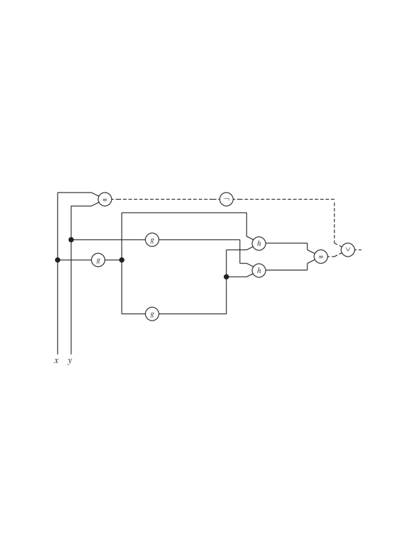
After removing applications of function symbol $g$:

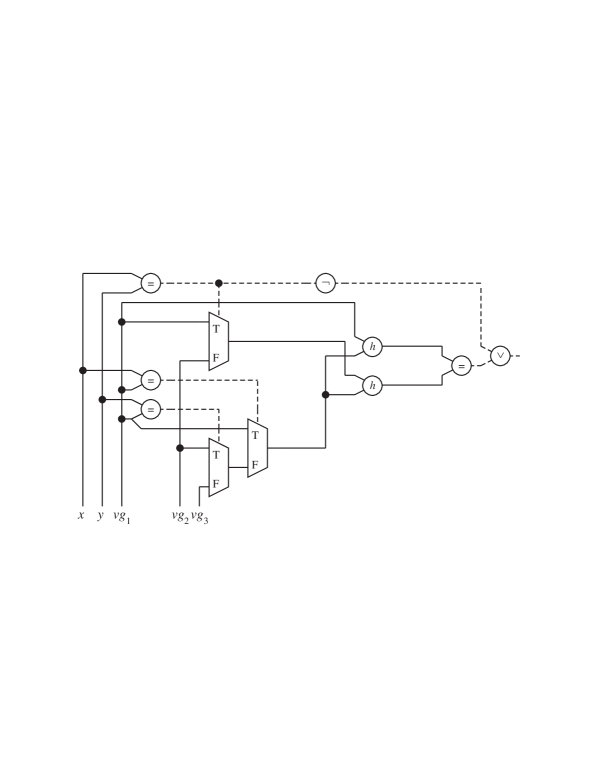
After removing applications of function symbol $h$:

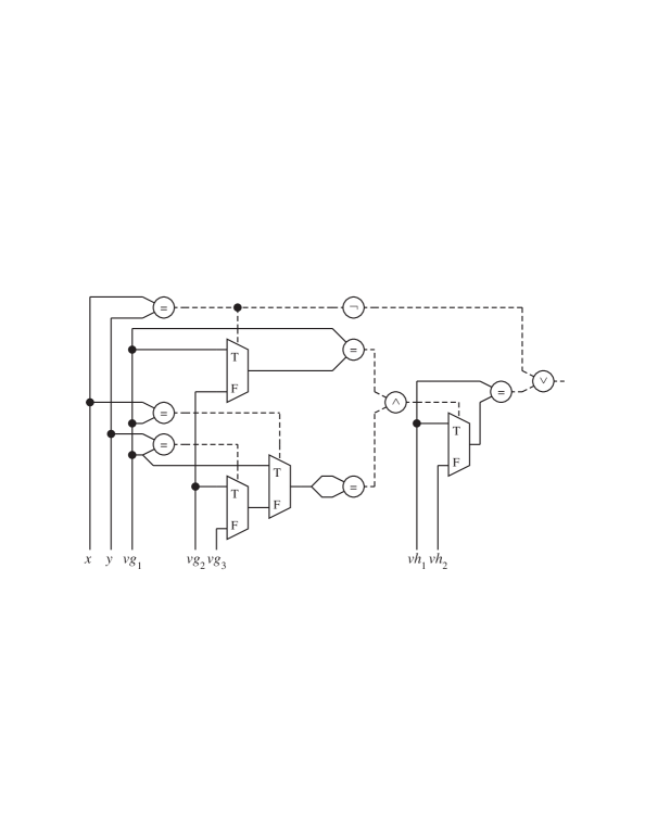
Figure 4: Removing Function Applications from $F_{\rm eg}$.

We demonstrate our technique for replacing function applications by domain variables using formula $F_{\rm eg}$ (Equation 1) as an example, as illustrated in Figure 4. First consider the three applications of function symbol $g$: $g(x)$, $g(y)$, and $g(g(x))$, which we identify as terms $T_{1}$, $T_{2}$, and $T_{3}$, respectively. Let ${\it vg}_{1}$, ${\it vg}_{2}$, and ${\it vg}_{3}$ be new domain variables. We generate new terms $U_{1}$, $U_{2}$, and $U_{3}$ as follows:

$$U_{1} \doteq {\it vg}_{1}$$ (3)

$$U_{2} \doteq \mbox{{\rm{\it ITE}}}(y\!=\!x,{\it vg}_{1},{\it vg}_{2})$$

$$U_{3} \doteq \mbox{{\rm{\it ITE}}}(vg_{1}\!=\!x,{\it vg}_{1},\mbox{{\rm{\it ITE}}}(vg_{1}\!=\!y,{\it vg}_{2},{\it vg}_{3}))$$

We use variable $vg_{1}$, the translation of $g(x)$, to represent the argument to the outer application of function symbol $g$ in the term $g(g(x))$. In general, we must always process nested applications of a given function symbol working from the innermost to the outermost. Given terms $U_{1}$, $U_{2}$, and $U_{3}$, we eliminate the function applications by replacing each instance of $T_{i}$ in the formula by $U_{i}$ for $1\leq i\leq 3$, as shown in the middle part of Figure 4. We use multiplexors in our schematic diagrams to represent ITE operations.

$\mathrel{\approx_{I^{\prime}}}$	$I^{\prime}[U_{1}]$	$I^{\prime}[U_{2}]$	$I^{\prime}[U_{3}]$
$\{x\},\{y\},\{g(x)\}$	$1$	$2$	$3$
$\{x,y\},\{g(x)\}$	$1$	$1$	$3$
$\{x\},\{y,g(x)\}$	$1$	$2$	$2$
$\{x,g(x)\},\{y\}$	$1$	$2$	$1$
$\{x,y,g(x)\}$	$1$	$1$	$1$

Table 3: Possible valuations of terms in Equation 3 when each variable ${\it vg}_{i}$ is assigned value $i$.

Observe that as we consider interpretations with different values for variables ${\it vg}_{1}$, ${\it vg}_{2}$, and ${\it vg}_{3}$ in Equation 3, we implicitly cover all values that an interpretation of function symbol $g$ in formula $F_{\rm eg}$ may yield for the three arguments. The nested ITE structure shown in Equation 3 enforces functional consistency. For example, consider an arbitrary interpretation $I$ of the symbols in $F_{\rm eg}$. Define interpretation $I^{\prime}$ to be identical to $I$ for the symbols in $F_{\rm eg}$ and in addition to assign values $1$, $2$, and $3$ to domain variables ${\it vg}_{1}$, ${\it vg}_{2}$, and ${\it vg}_{3}$, respectively. Table 3 shows the possible valuations of the three terms of Equation 3 under $I^{\prime}$. For each possible partitioning by $I^{*}$ of arguments $x$, $y$, and $g(x)$ into equivalence classes, we get $I^{\prime}[U_{i}]=I^{\prime}[U_{j}]$ if an only if the arguments to function application terms $T_{i}$ and $T_{j}$ are equal under $I$.

We remove the two applications of function symbol $h$ by a similar process. That is, we introduce two new domain variables $vh_{1}$ and $vh_{2}$. We replace the first application of $h$ by ${\it vh}_{1}$ and the second by an ITE term that compares the arguments of the two function applications, yielding $vh_{1}$ if they are equal and ${\it vh}_{2}$ if they are not. The final form is illustrated in the bottom part of Figure 4. The translation of predicate applications is similar, introducing a new propositional variable for each application. After removing all applications of function and predicate symbols of nonzero order, we are left with a formula $F_{\rm eg}^{*}$ containing only domain and propositional variables.

4.2 Algorithm for Eliminating Function and Predicate Applications

The general translation procedure follows the form shown for our example. It iterates through the function and predicate symbols of nonzero order. On each iteration it eliminates all occurrences of a given symbol. At the end we are left with a formula containing only domain and propositional variables.

Initial p-formula showing $f$-order contours:

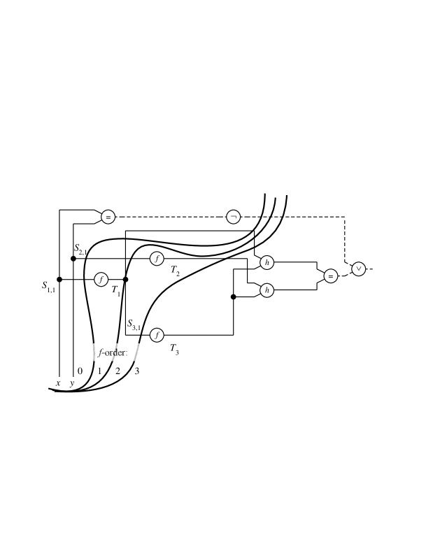
After removing applications of function symbol $f$:

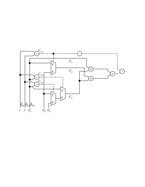
Figure 5: Illustration of Function Application Removal

The following is a detailed description of the process required to eliminate all instances of a single function symbol $f$ having order $k>0$ from a formula $G$. We use the variant of formula $F_{\rm eg}$ shown schematically at the top of Figure 5. In this variant, we have replaced function symbol $g$ with $f$. In the sequel, if $E$ is an expression and $T$ and $U$ are terms, we will write $E[T\leftarrow U]$ for the result of substituting $U$ for each instance of $T$ in $E$. Let $T_{1},\ldots,T_{n}$ denote the syntactically distinct terms occurring in formula $G$ having the application of $f$ as the top level operation. We refer to these as “$f$-application” terms. Let the arguments to $f$ in $f$-application term $T_{i}$ be the terms $S_{i,1},\ldots,S_{i,k}$, so that $T_{i}$ has the form $f(S_{i,1},\ldots,S_{i,k})$. Assume the terms $T_{1},\ldots,T_{n}$ are ordered such that if $T_{i}$ occurs as a subexpression of $T_{j}$ then $i<j$. In our example the $f$-application terms are: $T_{1}\doteq f(x)$, $T_{2}\doteq f(y)$ and $T_{3}\doteq f(f(x))$. These terms have arguments: $S_{1,1}\doteq x$, $S_{2,1}\doteq y$, and $S_{3,1}\doteq f(x)$.

The translation processes the $f$-application terms in order, such that on step $i$ it replaces all occurrences of the $i^{\mbox{\small th}}$ application of function symbol $f$ by a nested ITE term. Let ${\it vf}_{1},\ldots,{\it vf}_{n}$ be a new set of domain variables not occurring in $F$. We use these to encode the possible values returned by the $f$-application terms.

For any subexpression $E$ in $G$ define its integer-valued $f$-order, denoted $o_{f}(E)$, as the highest index $i$ of an $f$-application term $T_{i}$ occurring in $E$. If no $f$-application terms occur in $E$, its $f$-order is defined to be 0. By our ordering of the $f$-application terms, any argument $S_{i,l}$ to $f$-application term $T_{i}$ must have $o_{f}(S_{i,l})<o_{f}(T_{i})$, and therefore $o_{f}(T_{i})=i$. For example, the contour lines shown in Figure 5 partition the operators according to their $f$-order values.

The transformations performed in replacing applications of function symbol $f$ can be expressed by defining the following recurrence for any subexpression $E$ of $G$:

$$\begin{array}[]{rcll}E^{(0)}&\doteq&E\\ E^{(i)}&\doteq&E^{(i-1)}[T^{(i-1)}_{i}\leftarrow U_{i}],&1\leq i\leq n\\ \hat{E}&\doteq&E^{(m)},&\mbox{where}\;m=o_{f}(E)\\ \end{array}$$ (4)

In this equation, term $T^{(i-1)}_{i}$ is the form of the $i^{\mbox{\small th}}$ $f$-application term $T_{i}$ after all but the topmost application of $f$ have been eliminated. Term $U_{i}$ is a nested ITE structure encoding the possible values returned by $T_{i}$ while enforcing its consistency with earlier applications. $U_{i}$ does not contain any applications of function symbol $f$. For a subexpression $E$ with $o_{f}(E)=m$, its form $E^{(m)}$ will contain no applications of function symbol $f$. We denote this form as $\hat{E}$. Observe that for any $i>o_{f}(E)$, term $T^{(i-1)}_{i}$ does not occur in $E^{(i)}$, and hence $E^{(i)}=\hat{E}$ for all $i\geq o_{f}(E)$. Observe also that for $f$-application term $T_{i}$, we have $\hat{T}_{i}=T^{(i)}_{i}=U_{i}$.

$U_{i}$ is defined in terms of a recursively-defined term $V_{i,j}$ as follows:

$$\begin{array}[]{rcll}V_{i,i}&\doteq&{\it vf}_{i},&1\leq i\leq n\\ V_{i,j}&\doteq&\mbox{{\rm{\it ITE}}}(C_{i,j},{\it vf}_{j},V_{i,j+1}),&1\leq j<i\leq n\\ U_{i}&\doteq&V_{i,1},&1\leq i\leq n\\ \end{array}$$ (5)

where for each $j<i$, formula $C_{i,j}$ is true iff the (transformed) arguments to the top-level application of $f$ in the terms $T_{i}$ and $T_{j}$ have the same values:

$$C_{i,j}\;\;\;\doteq\;\;\;\bigwedge_{1\leq l\leq k}\hat{S}_{i,l}\!=\!\hat{S}_{j,l}$$ (6)

Observe that the recurrence of Equation 5 is well-defined, since for all argument terms of the form $S_{j,l}$ for $1\leq j\leq i$ and $1\leq l\leq k$, we have $o_{f}(S_{j,l})<i$, and hence terms of the form $\hat{S}_{j,l}$ and $\hat{S}_{i,l}$, as well as term $V_{i,j+1}$ are available when we define $V_{i,j}$.

The lower part of Figure 5 shows the result of removing the three applications of $f$ from our example formula. First, we have $U_{1}\doteq{\it vf}_{1}$, giving translated function arguments: $\hat{S}_{1,1}\doteq x$, $\hat{S}_{2,1}\doteq y$, and $\hat{S}_{3,1}\doteq{\it vf}_{1}$. The comparison formulas are then: $C_{2,1}\doteq(y\!=\!x)$, $C_{3,1}\doteq({\it vf}_{1}\!=\!x)$, and $C_{3,2}\doteq({\it vf}_{1}\!=\!y)$. From these we get translated terms:

$$U_{2} \doteq \mbox{{\rm{\it ITE}}}(y\!=\!x,{\it vf}_{1},{\it vf}_{2})$$

$$U_{3} \doteq \mbox{{\rm{\it ITE}}}({\it vf}_{1}\!=\!x,{\it vf}_{1},\mbox{{\rm{\it ITE}}}({\it vf}_{1}\!=\!y,{\it vf}_{2},{\it vf}_{3}))$$

We can see that formula $\hat{G}\doteq G^{(n)}$ will no longer contain any applications of function symbol $f$. We will show that $\hat{G}$ is universally valid if and only if $G$ is.

In the following correctness proofs, we will use a fundamental principle relating syntactic substitution and expression evaluation:

Proposition 1

For any expression $E$, pair of terms $T$, $U$, and interpretation $I$ of all of the symbols in $E$, $T$, and $U$, if $I[T]=I[U]$ then $I[E[T\leftarrow U]]=I[E]$.

We will also use the following characterization of Equation 5. For value $i$ such that $1\leq i\leq n$ and for interpretation $I$ of the symbols in $U_{i}$, we define the least matching value of $i$ under interpretation $I$, denoted ${\it lm}_{I}(i)$, as the minimum value $j$ in the range $1\leq j\leq i$ such that $I[\hat{S}_{j,l}]=I[\hat{S}_{i,l}]$ for all $l$ in the range $1\leq l\leq k$. Observe that this value is well defined, since $i$ forms a feasible value for $j$ in any case.

Lemma 3

For any interpretation $I$, $I[U_{i}]=I({\it vf}_{j})$, where $j={\it lm}_{I}(i)$.

Proof: For value $m$ in the range $1\leq m\leq i$ define ${\it lm}_{I}(m,i)$ as the minimum value of $j$ in the range $m\leq j\leq i$ such that $I[\hat{S}_{j,l}]=I[\hat{S}_{i,l}]$ for all $l$ in the range $1\leq l\leq k$. By this definition ${\it lm}_{I}(i)={\it lm}_{I}(1,i)$. Observe also that if $j={\it lm}_{I}(m,i)$ then $I[C_{i,j}]={\bf true}$. In addition, for any value $m^{\prime}$ in the range $m\leq m^{\prime}\leq i$, if ${\it lm}_{I}(m,i)\geq m^{\prime}$, then ${\it lm}_{I}(m,i)={\it lm}_{I}(m^{\prime},i)$.

We prove by induction on $m$ that $I[V_{i,m}]=I({\it vf}_{j})$, where $j={\it lm}_{I}(m,i)$. The base case of $m=i$ is trivial, since ${\it lm}_{I}(i,i)=i$, and $V_{i,i}={\it vf}_{i}$.

Assuming the property holds for $m+1$, we consider two possibilities. First, if ${\it lm}_{I}(m,i)=m$, we have $I[C_{i,m}]={\bf true}$, and hence the top-level ITE operation in $V_{i,m}$ (Equation 5) will select its first term argument ${\it vf}_{m}$, giving $I[V_{i,m}]=I({\it vf}_{m})$. On the other hand, if ${\it lm}_{I}(m,i)>m$, we must have $I[C_{i,m}]={\bf false}$, and hence the top-level ITE operation in $V_{i,m}$ will select its second term argument $V_{i,m+1}$, giving $I[V_{i,m}]=I[V_{i,m+1}]$, which by the inductive hypothesis equals $I({\it vf}_{j})$ for $j={\it lm}_{I}(m+1,i)$. Since ${\it lm}_{I}(m,i)\geq m+1$, we must also have ${\it lm}_{I}(m,i)={\it lm}_{I}(m+1,i)$, and hence $I[V_{i,m}]=I({\it vf}_{j})$, where $j={\it lm}_{I}(m,i)$.

Since $U_{i}$ is defined as $V_{i,1}$, our induction argument proves that $I[U_{i}]=I({\it vf}_{j})$ for $j={\it lm}_{I}(1,i)={\it lm}_{I}(i)$. $\Box$

Lemma 4

Any interpretation $J$ of the symbols in $G$ can be extended to an interpretation $\hat{J}$ of the symbols in both $G$ and $\hat{G}$ such that for every subexpression $E$ of $G$, $\hat{J}[\hat{E}]=\hat{J}[E]=J[E]$.

Proof: We provide a somewhat more general construction of $\hat{J}$ than is required for the proof of this lemma in anticipation of using this construction in the proof of Lemma 6. Given $J$ defined over domain ${\cal D}$, we define $\hat{J}$ over a domain $\hat{{\cal D}}$ such that $\hat{{\cal D}}\supseteq{\cal D}$.

We define $\hat{J}$ for the function and predicate symbols occurring in $G$ based on their definitions in $J$. For any function symbol $f$ in $G$ having ${\it ord}(f)=k$, and any argument values $x_{1},\ldots,x_{k}\in{\cal D}$, we define $\hat{J}(f)(x_{1},\ldots,x_{k})\doteq J(f)(x_{1},\ldots,x_{k})$. For argument values $x_{1},\ldots,x_{k}\in\hat{{\cal D}}$ such that for some $i$, $x_{i}\not\in{\cal D}$, we let $\hat{J}(f)(x_{1},\ldots,x_{k})$ be an arbitrary domain value. Similarly, for predicate symbol $p$, we define $\hat{J}(p)$ to yield the same value as $J(p)$ for arguments in ${\cal D}$ and to yield an arbitrary truth value when at least one argument is not in ${\cal D}$.

One can readily see that $\hat{J}[E]=J[E]$ for every subexpression $E$ of $G$. This takes care of the second equality in the statement of the lemma, and hence we can concentrate on the relation between $\hat{J}[\hat{E}]$ and $\hat{J}[E]$ for the remainder of the proof.

Recall that ${\it vf}_{1},\ldots,{\it vf}_{n}$ are the domain variables introduced when generating the nested ITE terms $U_{1},\ldots U_{n}$. Our strategy is to define interpretations of these variables such that each $U_{i}$ mimics the behavior of the original $f$-application term $T_{i}$ in $G$.

We consider two cases. For the case where ${\it lm}_{\hat{J}}(i)=i$, we define $\hat{J}({\it vf}_{i})=\hat{J}[T_{i}]$, i.e., the value of the $i^{\mbox{\small th}}$ $f$-application term in $G$ under $J$. Otherwise, we let $\hat{J}({\it vf}_{i})$ be an arbitrary domain value—we will show that its value does not affect the valuation of any expression $\hat{E}$ in $\hat{G}$ having a counterpart $E$ in $G$.

We argue by induction on $i$ that $\hat{J}[E^{(i)}]=\hat{J}[E]$ for any subexpression $E$ of $G$. For the case where $o_{f}(E)\leq i$, this hypothesis implies that $\hat{J}[\hat{E}]=\hat{J}[E]$. The base case of $i=0$ is trivial, since $E^{(0)}$ is defined to be $E$.

Suppose that for every $j$ in the range $1\leq j<i$ and every subexpression $D$ of $G$, we have $\hat{J}[{D}^{(j)}]=\hat{J}[D]$, and consequently that $\hat{J}[\hat{D}]=\hat{J}[D]$ for the case where $o_{f}(D)<i$. We must show that for every subexpression $E$ of $G$, we have $\hat{J}[E^{(i)}]=\hat{J}[E]$.

We first focus our attention on term $T_{i}$ in $G$ and its counterpart $U_{i}$ in $\hat{G}$, showing that $\hat{J}[U_{i}]=\hat{J}[T_{i}]$. The $f$-application terms for all $j$ such that $j<i$ have $o_{f}(T_{j})=j<i$, and hence we can assume that $\hat{J}[U_{j}]=\hat{J}[T_{j}]$ for these values of $j$. Furthermore, any argument $S_{j,l}$ to an $f$-application term for $j\leq i$ and $1\leq l\leq k$ has $o_{f}(S_{j,l})<j\leq i$, and hence we can assume $\hat{J}[\hat{S}_{j,l}]=\hat{J}[S_{j,l}]$.

We consider two cases: ${\it lm}_{\hat{J}}(i)=i$, and ${\it lm}_{\hat{J}}(i)<i$. In the former case, we have by Lemma 3 that $\hat{J}[U_{i}]=\hat{J}({\it vf}_{i})$. Our definition of $\hat{J}({\it vf}_{i})$ gives $\hat{J}[U_{i}]=\hat{J}({\it vf}_{i})=\hat{J}[T_{i}]$. Otherwise, suppose that ${\it lm}_{\hat{J}}(i)=j<i$. Lemma 3 shows that $\hat{J}[U_{i}]=\hat{J}({\it vf}_{j})$. We can see that ${\it lm}_{\hat{J}}(j)=j$, and hence $\hat{J}({\it vf}_{j})$ is defined to be $\hat{J}[T_{j}]$. By the definition of ${\it lm}$ we have $\hat{J}[\hat{S}_{j,l}]=\hat{J}[\hat{S}_{i,l}]$ for $1\leq l\leq k$. By the induction hypothesis we have $\hat{J}[\hat{S}_{j,l}]=\hat{J}[S_{j,l}]$, since $o_{f}(S_{j,l})<i$, and similarly that $\hat{J}[\hat{S}_{i,l}]=\hat{J}[S_{i,l}]$. By transitivity we have $\hat{J}[S_{j,l}]=\hat{J}[S_{i,l}]$ for all $l$ such that $1\leq l\leq k$, i.e., the arguments to $f$-application terms $T_{j}$ and $T_{i}$ have equal valuations under $J$. Function consistency requires that $\hat{J}[T_{j}]=\hat{J}[T_{i}]$. From this we can conclude that $\hat{J}[U_{i}]=\hat{J}[U_{j}]=\hat{J}[T_{j}]=\hat{J}[T_{i}]$. Combining these cases gives $\hat{J}[U_{i}]=\hat{J}[T_{i}]$.

For any subexpression $E$ its form $E^{(i)}$ differs from $E^{(i-1)}$ only in that all instances of term $T^{(i-1)}_{i}$ have been replaced by $U_{i}$. We have just argued that $\hat{J}[U_{i}]=\hat{J}[T_{i}]$, and by the induction hypothesis we have that $\hat{J}[T^{(i-1)}_{i}]=\hat{J}[T_{i}]$, giving by transitivity that $\hat{J}[T^{(i-1)}_{i}]=\hat{J}[U_{i}]$. Proposition 1 implies that $\hat{J}[E^{(i)}]=\hat{J}[E^{(i-1)}]$, and our induction hypothesis gives $\hat{J}[E^{(i-1)}]=\hat{J}[E]$. By transitivity we have $\hat{J}[E^{(i)}]=\hat{J}[E]$.

To complete the proof, we observe that our induction argument implies that for any subexpression $E$ of $G$, $\hat{J}[E^{(m)}]=\hat{J}[E]$, including for the case where $m=o_{f}(E)$, giving $\hat{J}[\hat{E}]=\hat{J}[E^{(m)}]=\hat{J}[E]$. $\Box$

Lemma 5

Any interpretation $\hat{J}$ of the symbols in $\hat{G}$ can be extended to an interpretation $J$ of the symbols in both $\hat{G}$ and $G$ such that for every subexpression $E$ of $G$, $J[E]=J[\hat{E}]=\hat{J}[\hat{E}]$ .

Proof: We define $J$ to be identical to $\hat{J}$ for any symbol occurring in $\hat{G}$. This implies that $J[\hat{E}]=\hat{J}[\hat{E}]$ for every subexpression $E$ of $G$. This takes care of the second equality in the statement of the lemma, and hence we can concentrate on the relation between $J[E]$ and $J[\hat{E}]$ for the remainder of the proof.

For function symbol $f$, we define $J(f)(x_{1},\ldots,x_{k})$ for domain elements $x_{1},\ldots,x_{k}$ as follows. Suppose there is some value $j$ such that $x_{l}=J[\hat{S}_{j,l}]$ for all $l$ such that $1\leq l\leq k$, and such that $j={\it lm}_{\hat{J}}(j)$. Then we define $J(f)(x_{1},\ldots,x_{k})$ to be $J({\it vf}_{j})$. If no such value of $j$ exists, we let $J(f)(x_{1},\ldots,x_{k})$ be some arbitrary domain value.

We argue by induction on $i$ that $J[E]=J[E^{(i)}]$ for any subexpression $E$ of $G$. For the case where $o_{f}(E)\leq i$, this hypothesis implies that $J[E]=J[\hat{E}]$. The base case of $i=0$ is trivial, since $E^{(0)}$ is defined to be $E$.

Suppose that for every $j$ in the range $1\leq j<i$ and every subexpression $D$ of $G$, we have $J[D]=J[{D}^{(i)}]$, and consequently that $J[D]=J[\hat{D}]$ for the case where $o_{f}(D)<i$. We must show that for every subexpression $E$ of $G$, we have $J[E]=J[E^{(i)}]$.

We focus initially on term $T_{i}$ in $G$ and its counterpart $U_{i}$ in $\hat{G}$, showing that $J[T_{i}]=J[U_{i}]$. Any $f$-application term $T_{j}$ for $j<i$ has $o_{f}(T_{j})=j<i$, and hence we can assume that $J[T_{j}]=J[\hat{T}_{j}]$. Furthermore, any argument $S_{j,l}$ to an $f$-application term for $j\leq i$ and $1\leq l\leq k$ has $o_{f}(S_{j,l})<j\leq i$, and hence we can assume that $J[S_{j,l}]=J[\hat{S}_{j,l}]$.

We consider two cases: ${\it lm}_{\hat{J}}(i)=i$, and ${\it lm}_{\hat{J}}(i)<i$. In the former case, we have by Lemma 3 that $J[U_{i}]=J({\it vf}_{i})$. In addition, $J(f)$ is defined such that $J[T_{i}]=J(f)(J[S_{i,1}],\ldots,J[S_{i,k}])=J(f)(J[\hat{S}_{i,1}],\ldots,J[\hat{S}_{i,k}])=J({\it vf}_{i})$, giving $J[T_{i}]=J({\it vf}_{i})=J[U_{i}]$. Otherwise, suppose that ${\it lm}_{J}(i)=j<i$. Lemma 3 shows that $J[U_{i}]=J({\it vf}_{j})$. We can see that ${\it lm}_{\hat{J}}(j)=j$, and hence $J(f)$ is defined such that $J(f)(J[\hat{S}_{j,1}],\ldots,J[\hat{S}_{j,k}])=J({\it vf}_{j})$. For any $l$ such that $1\leq l\leq k$, we also have by the definition of ${\it lm}$ that $J[\hat{S}_{j,l}]=J[\hat{S}_{i,l}]$. By the induction hypothesis we have $J[S_{j,l}]=J[\hat{S}_{j,l}]$, since $o_{f}(S_{j,l})<i$, and similarly that $J[S_{i,l}]=J[\hat{S}_{i,l}]$. By transitivity we have $J[S_{j,l}]=J[S_{i,l}]$, i.e., the arguments to $f$-application terms $T_{j}$ and $T_{i}$ have equal valuations under $J$. Functional consistency requires that $J[T_{j}]=J[T_{i}]$. Putting this together gives $J[T_{i}]=J[T_{j}]=J(f)(J[S_{j,1}],\ldots,J[S_{j,k}])=J(f)(J[\hat{S}_{j,1}],\ldots,J[\hat{S}_{j,k}])=J({\it vf}_{j})=J[U_{i}]$.

For any subexpression $E$ its form $E^{(i)}$ differs from $E^{(i-1)}$ only in that all instances of term $T^{(i-1)}_{i}$ have been replaced by $U_{i}$. We have just argued that $J[T_{i}]=J[U_{i}]$, and by the induction hypothesis we have that $J[T_{i}]=J[T^{(i-1)}_{i}]$, giving by transitivity that $J[T^{(i-1)}_{i}]=J[U_{i}]$. Proposition 1 implies that $J[E^{(i-1)}]=J[E^{(i)}]$, and our induction hypothesis gives $J[E]=J[E^{(i-1)}]$. By transitivity we have $J[E]=J[E^{(i)}]$.

To complete the proof, we observe that our induction argument implies that for any subexpression $E$ of $G$, $J[E]=J[E^{(m)}]$, including for the case where $m=o_{f}(E)$, giving $J[E]=J[E^{(m)}]=J[\hat{E}]$. $\Box$

An application of a predicate symbol having nonzero order can be removed by a similar process, using newly generated propositional variables to encode the possible values returned by the predicate applications. By an argument similar to that made in Lemma 4, we can extend an interpretation to include interpretations of the propositional variables such that the original and the transformed formulas have identical valuations. Conversely, by an argument similar to that made in Lemma 5, we can extend an interpretation to include an interpretation of the original predicate symbol such that the original and the transformed formulas have identical valuations.

Suppose formula $F$ contains applications $m$ different function and predicate symbols of nonzero order. Starting with $F_{0}\doteq F$, we can generate a sequence of formulas $F_{0},F_{1},\ldots,F_{m}$. Each formula $F_{i}$ is generated from its predecessor $F_{i-1}$ by letting $G=F_{i}$ and $F_{i+1}=\hat{G}$ in our technique to eliminate all instances of the $i^{\mbox{\small th}}$ function or predicate symbol. Let $F^{*}\doteq F_{m}$ denote the formula that will result once we have eliminated all applications of function and predicate symbols having nonzero order.

Theorem 3

For EUF formula $F$, the transformation process described above yields a formula $F^{*}$ such that $F$ is universally valid if and only if $F^{*}$ is universally valid.

Proof: If: Assume $F^{*}$ is universally valid, and consider any interpretation $I$ of the symbols in $F$. We construct a sequence of interpretations $I=I_{0},I_{1},\ldots,I_{m}$, where each interpretation $I_{i}$ is generated by extending its predecessor $I_{i-1}$ by letting $J=I_{i-1}$ and $I_{i}=\hat{J}$ in Lemma 4 or a similar one for predicate applications. The effect is to include in $I_{i}$ interpretations of the domain or propositional variables introduced when eliminating the $i^{\mbox{\small th}}$ function or predicate symbol. We then define interpretation $I^{*}$ to be identical to $I_{m}$ for every variable appearing in $F^{*}$. By induction, we have $I^{*}[F^{*}]=I[F]$. Since $F^{*}$ is universally valid, we have $I[F]=I^{*}[F^{*}]={\bf true}$. Since this construction can be performed for any interpretation $I$, $F$ must also be universally valid.

Only if: Assume $F$ is universally valid. Starting with an interpretation $I^{*}$ of the domain and propositional variables of $F^{*}$, we can define a sequence of interpretations $I^{*}=I_{m},I_{m-1},\ldots,I_{0}$, using the construction in the proof of Lemma 5 (or a similar one for predicate applications) to generate an interpretation of each function or predicate symbol in $F$. We then define interpretation $I$ to be identical to $I_{0}$ for every function or predicate symbol appearing in $F$. By induction, we have $I[F]=I^{*}[F^{*}]$. Since $F$ is universally valid, we have $I^{*}[F^{*}]=I[F]={\bf true}$. Since this construction can be performed for any interpretation $I^{*}$, $F^{*}$ must also be universally valid. $\Box$

4.3 Assigning Distinct Values to Variables Representing P-Function Applications

Suppose we are given a PEUF p-formula $F$. We can also consider this to be a formula in EUF and hence apply the function and predicate application elimination procedure just described to derive a formula $F^{*}$ containing only domain and propositional variables. For each function symbol $f$ in $F$, we will introduce a series of domain variables ${\it vf}_{1},\ldots,{\it vf}_{n}$. We will show that if $f$ is a p-function symbol, then our decision procedure can exploit maximal diversity by considering only interpretations that assign distinct values to the ${\it vf}_{1},\ldots,{\it vf}_{n}$. More precisely, we need only consider interpretations that are diverse for these variables when deciding the validity of $F$. This property holds even if the variables ${\it vf}_{1},\ldots,{\it vf}_{n}$ are not classified as p-function symbols in $F^{*}$.

For example, consider the formula created by eliminating function symbol $g$ from $F_{\rm eg}$, shown in the middle of Figure 4. By using an interpretation $I^{*}$ that assigns distinct values $1$, $2$, and $3$ to variables ${\it vg}_{1}$, ${\it vg}_{2}$, and ${\it vg}_{3}$ we generate distinct values for the terms $U_{1}$, $U_{2}$, and $U_{3}$ (Equation 3), except when there are matches between the arguments $x$, $y$, and ${\it vg}_{1}$. On the other hand, our encoding still considers the possibility that the arguments to the different applications of $g$ may match under some interpretations, in which case the function results should match as well. Observe that the equations $x\!=\!{\it vg}_{1}$ and $y\!=\!{\it vg}_{1}$ control ITEs in the transformed formula. Nonetheless, we will show that we can prove universal validity by considering only diverse interpretations of ${\it vg}_{1}$.

To show this formally, consider the effect of replacing all instances of a function symbol $f$ in a formula $G$ by nested ITE terms, as described earlier, yielding a formula $\hat{G}$ with new domain variables ${\it vf}_{1},\ldots,{\it vf}_{n}$. We first show that when we generate these variables while eliminating p-function applications, we can assume they have a diverse interpretation.

Lemma 6

Let $\Sigma$ be a subset of the symbols in $G$, and let $\hat{G}$ be the result of eliminating function symbol $f$ from $G$ by introducing new domain variables ${\it vf}_{1},\ldots,{\it vf}_{n}$. If $f\in\Sigma$, then for any interpretation $J$ that is diverse for $G$ with respect to $\Sigma$, there is an interpretation $\hat{J}$ that is diverse for $\hat{G}$ with respect to $\Sigma-\{f\}\cup\{{\it vf}_{1},\ldots,{\it vf}_{n}\}$ such that $\hat{J}[\hat{G}]=J[G]$.

Proof: Given interpretation $J$ defined over domain ${\cal D}$, we define interpretation $\hat{J}$ over a domain $\hat{{\cal D}}\doteq{\cal D}\cup\{z_{1},\ldots,z_{n}\}$. Each $z_{i}$ is a unique value, i.e., $z_{i}\not=z_{j}$ for any $i\not=j$, and $z_{i}\not\in{\cal D}$.

The proof of this lemma is based on a refinement of the proof of Lemma 4. Whereas the construction in the earlier proof assigned arbitrary values to the new domain variables in some cases, we select an assignment that is diverse in these variables. As in the construction in the proof of Lemma 4, we define $\hat{J}$ for any function or predicate symbol in $G$ to be identical to that of $J$ when the arguments are all elements of ${\cal D}$. When some argument is not in ${\cal D}$, we let the function (respectively, predicate) application yield an arbitrary domain (resp., truth) value.

For domain variable ${\it vf}_{i}$ introduced when generating term $U_{i}$, we consider two cases. For the case where ${\it lm}_{\hat{J}}(i)=i$, we define $\hat{J}({\it vf}_{i})=\hat{J}[T_{i}]$, i.e., the value of the $i^{\mbox{\small th}}$ $f$-application term in $G$ under $J$. For the case where ${\it lm}_{\hat{J}}(i)<i$, we define $\hat{J}({\it vf}_{i})=z_{i}$. We saw in the proof of Lemma 4 that we could assign arbitrary values in this latter case and still have $\hat{J}[\hat{G}]=J[G]$. In fact, for every subexpression $E$ of $G$, we have that its counterpart $\hat{E}$ in $\hat{G}$ satisfies $\hat{J}[\hat{E}]=J[E]$.

We must show that $\hat{J}$ is diverse for $\hat{G}$ with respect to $\Sigma-\{f\}\cup\{{\it vf}_{1},\ldots,{\it vf}_{n}\}$. We first observe that $\hat{J}$ is identical to $J$ for all function application terms in $G$, and hence $\hat{J}$ must be diverse with respect to $\Sigma$ for $G$. We also observe that $\hat{J}$ assigns to each variable ${\it vf}_{i}$ either a unique value $z_{i}$ or the value yielded by $f$-application term $T_{i}$ in $G$ under $\hat{J}$.

Suppose there were distinct variables ${\it vf}_{i}$ and ${\it vf}_{j}$ such that $\hat{J}[{\it vf}_{i}]=\hat{J}[{\it vf}_{j}]$. This could occur only for the case that $\hat{J}({\it vf}_{i})=\hat{J}[T_{i}]=\hat{J}[T_{j}]=\hat{J}({\it vf}_{j})$. Since $J$ is diverse, we can have $\hat{J}[T_{i}]=\hat{J}[T_{j}]$ only if ${\it lm}_{\hat{J}}(i)={\it lm}_{\hat{J}}(j)$. We cannot have both ${\it lm}_{\hat{J}}(i)=i$ and ${\it lm}_{\hat{J}}(j)=j$, and hence either ${\it vf}_{i}$ or ${\it vf}_{j}$ would have been assigned unique value $z_{i}$ or $z_{j}$, respectively. Thus, we can conclude that $\hat{J}[{\it vf}_{i}]\not=\hat{J}[{\it vf}_{j}]$ for distinct variables ${\it vf}_{i}$ and ${\it vf}_{j}$.

In addition, we must show that interpretation $\hat{J}$ does not create any matches between a new variable ${\it vf}_{i}$ and a function application term $T$ in $G$ that does not have $f$ as the topmost function symbol. Since $\hat{J}$ is diverse with respect to $\Sigma$ for $G$ and $f\in\Sigma$, any function application term $T$ in $G$ that does not have function symbol $f$ as its topmost symbol must have $\hat{J}[T]\not=\hat{J}[T_{i}]$ for all $1\leq i\leq n$. In addition, we have $\hat{J}[T]\not=z_{i}$ for all $1\leq i\leq n$. Hence, we must have $\hat{J}[T]\not=J({\it vf}_{i})$. $\Box$

We must also show that the variables introduced when eliminating g-function applications do not adversely affect the diversity of the other symbols.

Lemma 7

Let $\Sigma$ be a subset of the symbols in $G$, and let $\hat{G}$ be the result of eliminating function symbol $f$ from $G$ by introducing new domain variables ${\it vf}_{1},\ldots,{\it vf}_{n}$. If $f\not\in\Sigma$, then for any interpretation $J$ that is diverse for $G$ with respect to $\Sigma$, there is an interpretation $\hat{J}$ that is diverse for $\hat{G}$ with respect to $\Sigma$ such that $\hat{J}[\hat{G}]=J[G]$.

Proof: The proof of this lemma is based on a refinement of the proof of Lemma 4. Whereas the construction in the earlier proof assigned arbitrary values to some of the new domain variables, we select an assignment such that we do not inadvertently violate the diversity of the other function symbols.

We define $\hat{J}$ to be identical to $J$ for any symbol occurring in $G$. For each domain variable ${\it vf}_{i}$ introduced when generating term $U_{i}$, we define $\hat{J}({\it vf}_{i})=\hat{J}[T_{i}]$. This differs from the interpretation defined in the proof of Lemma 4 only in giving fixed interpretations of domain variables that could otherwise be arbitrary, and hence we have have $\hat{J}[\hat{G}]=J[G]$. In fact, for every subexpression $E$ of $G$, we have that its counterpart $\hat{E}$ in $\hat{G}$ satisfies $\hat{J}[\hat{E}]=J[E]$.

We must show that $\hat{J}$ is diverse for $\hat{G}$ with respect to $\Sigma$. We first observe that $\hat{J}$ is identical to $J$ for all function application terms in $G$, and hence $\hat{J}$ must be diverse for $G$ with respect to $\Sigma$. We also observe that $\hat{J}$ assigns to each variable ${\it vf}_{i}$ the value of $f$-application term $T_{i}$. For term $T$ having the application of function symbol $g\in\Sigma$ as the topmost operation, we must have $\hat{J}[\hat{T}]=\hat{J}[T]\not=\hat{J}[T_{i}]=J[{\it vf}_{i}]$. Hence, we are assured that the values assigned to the new variables under $\hat{J}$ do not violate the diversity of the interpretations of the symbols in $\Sigma$. $\Box$

Suppose we apply the transformation process of Theorem 3 to a p-formula $F$ to generate a formula $F^{*}$, and that in this process, we introduce a set of new domain variables $V$ to replace the applications of the p-function symbols. Let $\Sigma^{*}_{p}(F)$ be the union of the set of domain variables in $\Sigma_{p}(F)$ and $V$. That is, $\Sigma^{*}_{p}(F)$ consists of those domain variables in the original formula $F$ that were p-function symbols as well as the domain variables generated when replacing applications of p-function symbols. Let $\Sigma^{*}_{g}(F)$ be the domain variables in $F^{*}$ that are not in $\Sigma^{*}_{p}(F)$. These variables were either g-function symbols in $F$ or were generated when replacing g-function applications.

We observe that we can generate all maximally diverse interpretations of $F$ by considering only interpretations of the variables in $F^{*}$ that assign distinct values to the variables in $\Sigma^{*}_{p}(F)$:

Theorem 4

PEUF p-formula $F$ is universally valid if and only if its translation $F^{*}$ is true for every interpretation $I^{*}$ that is diverse over $\Sigma^{*}_{p}(F)$.

Proof: Only if: By Theorem 3, the universal validity of $F$ implies that of $F^{*}$, and hence it must be true for every interpretation.

If: The proof in the other direction follows by inducting on the number of function and predicate symbols in $F$ having nonzero order. For the induction step we use Lemma 6 when eliminating all applications of a p-function symbol, and Lemma 7 when eliminating all applications of a g-function symbol. When eliminating a predicate symbol, we do not introduce any new domain variables. $\Box$

4.3.1 Discussion

Initial formula:

After removing applications of function symbol $g$:

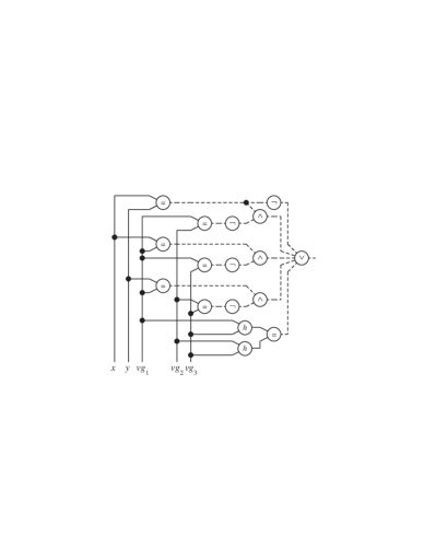
After removing applications of function symbol $h$:

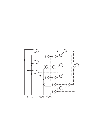
Figure 6: Ackermann’s Method for Replacing Function Applications in $F_{\rm eg}$.

Ackermann also describes a scheme for replacing function application terms by domain variables [Ack54]. His scheme simply replaces each instance of a function application by a newly-generated domain variable and then introduces constraints expressing functional consistency as antecedents to the modified formula. As an illustration, Figure 6 shows the result of applying his method to formula $F_{\rm eg}$ of Equation 1. First, we replace the three applications of function symbol $g$ with new domain variables ${\it vg}_{1}$, ${\it vg}_{2}$, and ${\it vg}_{3}$. To maintain functional consistency we add constraints

$$(x\!=\!y\Rightarrow{\it vg}_{1}\!=\!{\it vg}_{2})\land(x\!=\!{\it vg}_{1}\Rightarrow{\it vg}_{1}\!=\!{\it vg}_{3})\land(y\!=\!{\it vg}_{1}\Rightarrow{\it vg}_{2}\!=\!{\it vg}_{3})$$

as an antecedent to the modified g-formula. The result is shown in the middle of Figure 6, using Boolean connectives $\land$, $\lor$, and $\neg$ rather than $\Rightarrow$. In this diagram, the three constraints listed above form the middle three arguments of the final disjunction. A similar process is used to replace the applications of function symbol $h$, adding a fourth constraint ${\it vg}_{1}\!=\!{\it vg}_{2}\land{\it vg}_{3}\!=\!{\it vg}_{3}\Rightarrow{\it vh}_{1}\!=\!{\it vh}_{2}$. The result is shown at the bottom of Figure 6.

There is no clear way to exploit the maximal diversity with this translated form. For example, if we consider only diverse interpretations of variables ${\it vg}_{1}$, ${\it vg}_{2}$, and ${\it vg}_{3}$, we will fail to consider interpretations of the original g-formula for which $x$ equals $y$.

4.4 Using Fixed Interpretations of the Variables in $\Sigma^{*}_{p}(F)$

We can further simplify the task of determining universal validity by choosing particular domains of sufficient size and assigning fixed interpretations to the variables in $\Sigma^{*}_{p}(F)$. The next result follows from Theorem 4.

Corollary 1

Let ${\cal D}_{p}$ and ${\cal D}_{g}$ be disjoint subsets of domain ${\cal D}$ such that $|{\cal D}_{p}|\geq|\Sigma^{*}_{p}(F)|$ and $|{\cal D}_{g}|\geq|\Sigma^{*}_{g}(F)|$. Let $\alpha$ be any 1–1 mapping $\alpha\colon\Sigma^{*}_{p}(F)\rightarrow{\cal D}_{p}$. PEUF p-formula $F$ is universally valid if and only if its translation $F^{*}$ is true for every interpretation $I^{*}$ such that $I^{*}(v_{p})=\alpha(v_{p})$ for every variable $v_{p}\in\Sigma^{*}_{p}(F)$, and $I^{*}(v_{g})\in{\cal D}_{g}$ for every variable $v_{g}\in\Sigma^{*}_{g}(F)$.

Proof: Consider any interpretation $J^{*}$ of the variables in $\Sigma^{*}_{p}(F)\cup\Sigma^{*}_{g}(F)$ that is diverse over $\Sigma^{*}_{p}(F)$. We show that we can construct an isomorphic interpretation $I^{*}$ that satisfies the restrictions of the corollary.

Let ${\cal D}_{p}^{\prime}$ (respectively, ${\cal D}_{g}^{\prime}$) be the range of $J^{*}$ considering only variables in $\Sigma^{*}_{p}(F)$ (resp., $\Sigma^{*}_{g}(F)$). The function $J^{*}\colon\Sigma^{*}_{p}(F)\rightarrow{\cal D}_{p}^{\prime}$ must be a bijection and hence have an inverse ${J^{*}}^{-1}\colon{\cal D}_{p}^{\prime}\rightarrow\Sigma^{*}_{p}(F)$. Furthermore, we must have $|{\cal D}_{g}^{\prime}|\leq|\Sigma^{*}_{g}(F)|\leq|{\cal D}_{g}|$. Let $\sigma_{p}$ be the 1–1 mapping $\sigma_{p}\colon{\cal D}_{p}^{\prime}\rightarrow{\cal D}_{p}$ defined for any $z$ in ${\cal D}_{p}^{\prime}$, as $\sigma_{p}(z)=\alpha({J^{*}}^{-1}(z))$. Let $\sigma_{g}$ be an arbitrary 1–1 mapping $\sigma_{g}\colon{\cal D}_{g}^{\prime}\rightarrow{\cal D}_{g}$. We now define $I^{*}$ such that for any variable $v$ in $\Sigma^{*}_{p}(F)$ (respectively, $\Sigma^{*}_{g}(F)$) we have $I^{*}(v)$ equal to $\sigma_{p}(J^{*}(v))$ (resp., $\sigma_{g}(J^{*}(v))$). Finally, for any propositional variable $a$, we let $I^{*}(a)$ equal $J^{*}(a)$.

For any EUF formula, isomorphic interpretations will always yield identical valuations, giving $I^{*}[F^{*}]=J^{*}[F^{*}]$. Hence the set of interpretations satisfying the restrictions of the corollary form a sufficient set to prove the universal validity of $F^{*}$. $\Box$

5 Reductions to Propositional Logic

We present two different methods of translating a PEUF p-formula into a propositional formula that is tautological if and only if the original p-formula is universally valid. Both use the function and predicate elimination method described in the previous section so that the translation can be applied to a formula $F^{*}$ containing only domain and predicate variables. In addition, we assume that a subset of the domain variables $\Sigma^{*}_{p}(F)$ has been identified such that we need to encode only those interpretations that are diverse over these variables.

5.1 Translation Based on Bit Vector Interpretations

A formula such as $F^{*}$ containing only domain and propositional variables can readily be translated into one in propositional logic, using the set of bit vectors of some length $k$ greater than or equal to $\log_{2}m$ as the domain of interpretation for a formula containing $m$ domain variables [VB98]. Domain variables are represented with vectors of propositional variables. In this formulation, we represent a domain variable as a vector of propositional variables, where truth value ${\bf false}$ encodes bit value 0, and truth value ${\bf true}$ encodes bit value 1. In [VB98] we described an encoding scheme in which the $i^{\mbox{\small th}}$ domain variable is encoded as a bit vector of the form $\langle 0,\ldots,0,a_{i,k-1},\ldots,a_{i,0}\rangle$ where $k=\lceil\log_{2}i\rceil$, and each $a_{i,j}$ is a propositional variable. This scheme can be viewed as encoding interpretations of the domain variables over the integers where the $i^{\mbox{\small th}}$ domain variable ranges over the set $\{0,\ldots,i-1\}$ [PRSS99]. That is, it may equal any of its predecessors, or it may be distinct.

We then recursively translate $F^{*}$ using vectors of propositional formulas to represent terms. By this means we then reduce $F^{*}$ to a propositional formula that is tautological if and only if $F^{*}$, and consequently the original EUF formula $F$, is universally valid.

We can exploit positive equality by using fixed bit vectors, rather than vectors of propositional variables when encoding variables in $\Sigma^{*}_{p}(F)$. Furthermore, we can construct our bit encodings such that the vectors encoding variables in $\Sigma^{*}_{g}(F)$ never match the bit patterns encoding variables in $\Sigma^{*}_{p}(F)$. As an illustration, consider formula $F_{\rm eg}$ given by Equation 1 translated into formula $F_{\rm eg}^{*}$ as diagrammed at the bottom of Figure 4. We need encode only those interpretations of variables $x$, $y$, ${\it vg}_{1}$, ${\it vg}_{2}$, ${\it vg}_{3}$, ${\it vh}_{1}$, and ${\it vh}_{2}$ that are diverse respect to the last five variables. Therefore, we can assign 3-bit encodings to the seven variables as follows:

$x$	$\langle 0,0,0\rangle$
$y$	$\langle 0,0,a_{1,0}\rangle$
${\it vg}_{1}$	$\langle 0,1,0\rangle$
${\it vg}_{2}$	$\langle 0,1,1\rangle$
${\it vg}_{3}$	$\langle 1,0,0\rangle$
${\it vh}_{1}$	$\langle 1,0,1\rangle$
${\it vh}_{2}$	$\langle 1,1,0\rangle$

where $a_{1,0}$ is a propositional variable. This encoding uses the same scheme as [VB98] for the variables in $\Sigma^{*}_{g}(F)$ but uses fixed bit patterns for the variables in $\Sigma^{*}_{p}(F)$. As a consequence, we require just a single propositional variable to encode formula $F_{\rm eg}^{*}$.

As a further refinement, we could apply methods devised by Pnueli et al.  to reduce the size of the domains associated with each variable in $\Sigma^{*}_{g}(F)$ [PRSS99]. This will in turn allow us to reduce the number of propositional variables required to encode each domain variable in $\Sigma^{*}_{g}(F)$.

5.2 Translation Based on Pairwise Encodings of Term Equality

Goel et al.  [GSZAS98] describe a method for generating a propositional formula from an EUF formula, such that the propositional formula will be a tautology if and only if the EUF formula is universally valid. They first use Ackermann’s method to eliminate function applications of nonzero order [Ack54]. Then they introduce a propositional variable $e_{i,j}$ for each pair of domain variables $v_{i}$ and $v_{j}$ encoding the conditions under which the two variables have matching values. Finally, they generate a propositional formula in terms of the $e_{i,j}$ variables.

We provide a modified formulation of their approach that exploits the properties of p-formulas to encode only valuations under maximally diverse interpretations. As a consequence, we require $e_{i,j}$ variables only to express equality among those domain variables that represent g-term values in the original p-formula.

The propositional formula generated by either of these schemes does not enforce constraints among the $e_{i,j}$ variables due to the transitivity of equality, i.e., constraints of the form $e_{i,j}\land e_{j,k}\Rightarrow e_{i,k}$. As a result, in attempting to prove the formula is a tautology, a false “counterexamples” may be generated. We return to this issue later in this section

5.2.1 Construction of Propositional Formula

Starting with p-formula $F$, we apply our method of eliminating function applications to give a formula $F^{*}$ containing only domain and propositional variables. The domain variables in $F^{*}$ are partitioned into sets $\Sigma^{*}_{p}(F)$, corresponding to p-function applications in $F$, and $\Sigma^{*}_{g}(F)$ corresponding to g-function applications in $F$. Let us identify the variables in $\Sigma^{*}_{g}(F)$ as $\{v_{1},\ldots,v_{N}\}$, and the variables in $\Sigma^{*}_{p}(F)$ as $\{v_{N+1},\ldots,v_{N+M}\}$. We need encode only those interpretations that are diverse in this latter set of variables.

For values of $i$ and $j$ such that $1\leq i<j\leq N$, define propositional variables $e_{i,j}$ encoding the equality relation between variables $v_{i}$ and $v_{j}$. We require these propositional variables only for indices less than or equal to $N$. Higher indices correspond to variables in $\Sigma^{*}_{p}(F)$, and we can assume for any such variable $v_{i}$ that it will equal variable $v_{j}$ only when $i=j$.

For each term $T$ in $F^{*}$, and each $v_{i}$ with $1\leq i\leq N+M$, we generate formulas of the form ${\it enct}_{i}(T)$ for $1\leq i\leq N+M$ to encode the conditions under which the control g-formulas in the ITEs in term $T$ will be set so that value of $T$ becomes that of domain variable $v_{i}$. In addition, for each g-formula $G$ we define a propositional formula ${\it encf}(G)$ giving the encoded form of $G$. These formulas are defined by mutual recursion. The base cases are:

$$\begin{array}[]{rcll}{\it encf}({\bf true})&\doteq&{\bf true}\\ {\it encf}({\bf false})&\doteq&{\bf false}\\ {\it encf}(a)&\doteq&a,&\mbox{$a$ is a propositional variable}\\ {\it enct}_{i}(v_{i})&\doteq&{\bf true}\\ {\it enct}_{j}(v_{i})&\doteq&{\bf false},&\mbox{For $i\not=j$}\\ \end{array}$$

For the logical connectives, we define ${\it encf}$ in the obvious way:

$${\it encf}(\neg G_{1}) \doteq \neg{\it encf}(G_{1})$$

$${\it encf}(G_{1}\land G_{2}) \doteq {\it encf}(G_{1})\land{\it encf}(G_{2})$$

$${\it encf}(G_{1}\lor G_{2}) \doteq {\it encf}(G_{1})\lor{\it encf}(G_{2})$$

For ITE terms, we define ${\it enct}$ as:

$${\it enct}_{i}(\mbox{{\rm{\it ITE}}}(G,T_{1},T_{2})) \doteq {\it encf}(G)\land{\it enct}_{i}(T_{1})\;\;\lor\;\;\neg{\it encf}(G)\land{\it enct}_{i}(T_{2})$$

For equations, we define ${\it encf}(T_{1}\!=\!T_{2})$ to be

$${\it encf}(T_{1}\!=\!T_{2}) \doteq \bigvee_{1\leq i,j\leq N}{\it enct}_{i}(T_{1})\land e_{[i,j]}\land{\it enct}_{j}(T_{2})\;\;\lor\;\;\bigvee_{N+1\leq i\leq N+M}{\it enct}_{i}(T_{1})\land{\it enct}_{i}(T_{2})$$

where $e_{[i,j]}$ is defined for $1\leq i,j\leq N$ as:

$$e_{[i,j]} \doteq \left\{\begin{array}[]{ll}{\bf true}&i=j\\ e_{i,j}&i<j\\ e_{j,i}&i>j\end{array}\right.$$

Informally, Equation LABEL:equation-equation expresses the property that there are two ways for a pair of terms to be equal in an interpretation. The first way is if the two terms evaluate to the same variable, i.e., we have both ${\it enct}_{i}(T_{1})$ and ${\it enct}_{i}(T_{2})$ hold for some variable $v_{i}$. For $1\leq i\leq N$, the left hand part of Equation LABEL:equation-equation will hold since $e_{[i,i]}={\bf true}$. For $N+1\leq i\leq N$, the right hand part of Equation LABEL:equation-equation will hold. The second way is that two terms will be equal under some interpretation when they evaluate to two different variables $v_{i}$ and $v_{j}$ that have the same value. In this case we will have ${\it enct}_{i}(T_{1})$, ${\it enct}_{j}(T_{2})$, and $e_{[i,j]}$ hold, where $1\leq i,j\leq N$. Observe that Equation LABEL:equation-equation encodes only interpretations that are diverse over $\{v_{N+1},\ldots,v_{N+M}\}$. It makes use of the fact that when $N+1\leq i\leq N+M$, variable $v_{i}$ will equal variable $v_{j}$ only if $i=j$.

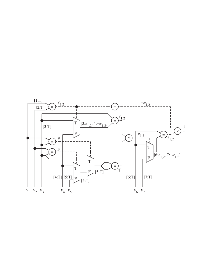
Figure 7: Encoding Example Formula in Propositional Logic. Each term $T$ is represented as a list giving the non-${\bf false}$ values of ${\it enct}_{i}(T)$.

As an example, Figure 7 shows an encoding of formula $F^{*}$ given in Figure 4, which was derived from the original formula $F$ shown in Figure 3. The variables in $\Sigma^{*}_{g}(F^{*})$ are $x$ and $y$. These are renamed as $v_{1}$ and $v_{2}$, giving $N=2$. The variables in $\Sigma^{*}_{p}(F^{*})$ are ${\it vg}_{1}$, ${\it vg}_{2}$, ${\it vg}_{3}$, ${\it vh}_{1}$, and ${\it vh}_{2}$. These are relabeled as $v_{3}$ through $v_{7}$, giving $M=5$. Each formula in the figure is annotated by a (simplified) propositional formula, while each term $T$ is annotated by a list with entries of the form $i\colon{\it enct}_{i}(T)$, for those entries such that ${\it enct}_{i}(T)\not={\bf false}$. We use the shorthand notation “T” for ${\bf true}$ and “F” for ${\bf false}$. Our encoding introduces a single propositional variable $e_{1,2}$. It can be seen that our method encodes only the interpretations for $F^{*}$ labeled as D1 and D2 in Table 2. When $e_{1,2}$ is false, we encode interpretation D2, in which $x\not=y$ and every function application term yields a distinct value. When $e_{1,2}$ is true, we encode interpretation D1, in which $x=y$ and hence we have $g(x)=g(y)$ and $h(g(x),g(g(x)))=h(g(y),g(g(y)))$.

In general, the final result of the recursive translation will be a propositional formula ${\it encf}(F^{*})$. The variables in this formula consist of the propositional variables that occur in $F^{*}$ as well as a subset of the variables of the form $e_{i,j}$. Nothing in this formula enforces the transitivity of equality. We will discuss in the next section how to impose transitivity constraints in a way that exploits the sparse structure of the equations. Other than transitivity, we claim that the translation ${\it encf}(F^{*})$ captures validity of $F^{*}$, and consequently the original p-formula $F$. For an interpretation $J$ over a set of propositional variables, including variables of the form $e_{i,j}$ for $1\leq i<j\leq N$, we say that $J$ obeys transitivity when for all $i$, $j$, and $k$ such that $1\leq i,j,k\leq N$ we have $J[e_{[i,j]}]\land J[e_{[j,k]}]\Rightarrow J[e_{[i,k]}]$.

To formalize the intuition behind the encoding, let $I^{*}$ be an interpretation of the variables in the translated formula $F^{*}$. For interpretation $I^{*}$, define ${\it sel}_{I^{*}}(T)$ to be a function mapping each term $T$ in $F^{*}$ to the index of the unique domain variable selected by the values of the ITE control g-formulas in $T$. That is, ${\it sel}_{I^{*}}(v_{i})\doteq i$, while ${\it sel}_{I^{*}}(\mbox{{\rm{\it ITE}}}(G,T_{1},T_{2}))$ is defined as ${\it sel}_{I^{*}}(T_{1})$ when $I^{*}[G]={\bf true}$ and as ${\it sel}_{I^{*}}(T_{2})$ when $I^{*}[G]={\bf false}$.

Proposition 2

For all interpretations $I^{*}$ of the variables in $F^{*}$ and any term $T$ occurring in $F^{*}$, if ${\it sel}_{I^{*}}(T)=i$, then $I^{*}[T]=I^{*}(v_{i})$.

Lemma 8

For any interpretation $I^{*}$ of the variables in $F^{*}$ that is diverse for $\Sigma^{*}_{p}(F)$, there is an interpretation $J$ of the variables in ${\it encf}(F^{*})$ that obeys transitivity and such that $J[{\it encf}(F^{*})]=I^{*}[F^{*}]$.

Proof: For each propositional variable $a$ occurring in $F^{*}$, we define $J(a)\doteq I^{*}(a)$. For each pair of variables $v_{i}$ and $v_{j}$ such that $1\leq i<j\leq N$, we define $J(e_{i,j})$ to be ${\bf true}$ iff $I^{*}(v_{i})=I^{*}(v_{j})$. We can see that $J$ must obey transitivity, because it is defined in terms of a transitive relation in $I^{*}$.

We prove the following hypothesis by induction on the expression depths:

1. For every formula $G$ in $F^{*}$: $J[{\it encf}(G)]=I^{*}[G]$.

2. For every term $T$ in $F^{*}$ and all $i$ such that $1\leq i\leq N+M$: $J[{\it enct}_{i}(T)]={\bf true}$ iff ${\it sel}_{I^{*}}(T)=i$.

The base cases hold as follows:

1. Formulas of the form ${\bf true}$, ${\bf false}$, and $a$ have ${\it encf}(G)=G$ and $J[G]=I^{*}[G]$.

2. Term $v_{j}$ has $J[{\it enct}_{i}(v_{j})]={\bf true}$ iff $j=i$, and ${\it sel}_{I^{*}}(v_{j})=i$ iff $j=i$.

Assuming the induction hypothesis holds for formulas $G_{1}$ and $G_{2}$, one can readily see that it will hold for formulas $\neg G_{1}$, $G_{1}\land G_{2}$, and $G_{1}\lor G_{2}$, by the definition of ${\it encf}$

Assuming the induction hypothesis holds for formula $G$ and for terms $T_{1}$ and $T_{2}$, consider term $T$ of the form $\mbox{{\rm{\it ITE}}}(G,T_{1},T_{2})$. For the case where $I^{*}[G]={\bf true}$, we have $I^{*}[T]=I^{*}[T_{1}]$, and also ${\it sel}_{I^{*}}(T)={\it sel}_{I^{*}}(T_{1})$. The induction hypotheses for $T_{1}$ gives $J[{\it enct}_{i}(T_{1})]={\bf true}$ iff ${\it sel}_{I^{*}}(T_{1})=i$. The induction hypothesis for $G$ gives $J[{\it encf}(G)]=I^{*}[G]={\bf true}$, and hence $J[{\it enct}_{i}(T)]=J[{\it enct}_{i}(T_{1})]$. From all this, we can conclude that $J[{\it enct}_{i}(T)]={\bf true}$ iff ${\it sel}_{I^{*}}(T)=i$. A similar argument holds when $I^{*}[G]={\bf false}$, but based on the induction hypothesis for $T_{2}$.

Finally, assuming the induction hypothesis holds for terms $T_{1}$ and $T_{2}$, consider the equation $T_{1}\!=\!T_{2}$. Suppose that ${\it sel}_{I^{*}}(T_{1})=i$ and ${\it sel}_{I^{*}}(T_{2})=j$. Our induction hypothesis for $T_{1}$ and $T_{2}$ give $J[{\it enct}_{i}(T_{1})]=J[{\it enct}_{j}(T_{2})]={\bf true}$. Suppose either $i>N$ or $j>N$. Then we will have $I^{*}(v_{i})=I^{*}(v_{j})$ iff $i=j$. In addition, the right hand part of Equation LABEL:equation-equation will hold under $J$ iff $i=j$. Otherwise, suppose that $1\leq i,j\leq N$. We will have $I^{*}(v_{i})=I^{*}(v_{j})$ iff $J[e_{[i,j]}]={\bf true}$. In addition, the left hand part of Equation LABEL:equation-equation will hold under $J$ iff $J[e_{[i,j]}]={\bf true}$ $\Box$

Lemma 9

For every interpretation $J$ of the variables in ${\it encf}(F^{*})$ that obeys transitivity, there is an interpretation $I^{*}$ of the variables in $F^{*}$ such that $I[F^{*}]=J[{\it encf}(F^{*})]$.

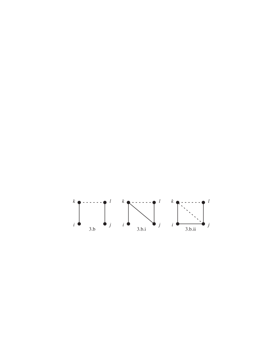
Figure 8: Case Analysis for Part 3b of Proof of Lemma 9. Solid lines denote equalities, while dashed lines denote inequalities.

Proof: We define interpretation $I^{*}$ over the domain of integers $\{1,\ldots,N+M\}$. For propositional variable $a$, we define $I^{*}(a)=J(a)$. For $1\leq j\leq N$ we let $I^{*}(v_{j})$ be the minimum value of $i$ such that $J[e_{[i,j]}]={\bf true}$. For $N<j\leq N+M$ we let $I^{*}(v_{j})=j$. Observe that this interpretation gives $I^{*}(v_{j})\leq j$ for all $j\leq N$, since $e_{[j,j]}={\bf true}$, and $I^{*}(v_{j})=j$ for $j>N$.

We claim that for $i\leq N$, if $I^{*}(v_{j})=i$, then we must have $I^{*}(v_{i})=i$ as well. If instead we had $I^{*}(v_{i})=k<i$, then we must have $J[e_{[k,i]}]={\bf true}$. Combining this with $J[e_{[i,j]}]={\bf true}$, the transitivity requirement would give $J[e_{[k,j]}]={\bf true}$, but this would imply that $I^{*}(v_{j})=k\not=i$.

We prove the following hypothesis by induction on the expression depths:

1. For every formula $G$ in $F^{*}$: $I^{*}[G]=J[{\it encf}(G)]$.

2. For every term $T$ in $F^{*}$ and all $i$ such that $1\leq i\leq N+M$: ${\it sel}_{I^{*}}(T)=i$ iff $J[{\it enct}_{i}(T)]={\bf true}$.

The base cases hold as follows:

1. Formulas of the form ${\bf true}$, ${\bf false}$, and $a$ have $G={\it encf}(G)$ and $I^{*}[G]=J[G]$.

2. Term $v_{j}$ has ${\it sel}_{I^{*}}(v_{j})=i$ iff $j=i$ and $J[{\it enct}_{i}(v_{j})]={\bf true}$ iff $j=i$.

Assuming the induction hypothesis holds for formula $G$ and for terms $T_{1}$ and $T_{2}$, consider term $T$ of the form $\mbox{{\rm{\it ITE}}}(G,T_{1},T_{2})$. For the case where $J[{\it encf}(G)]={\bf true}$, we have $J[{\it enct}_{i}(T)]=J[{\it enct}_{i}(T_{1})]$. The induction hypothesis for $T_{1}$ gives ${\it sel}_{I^{*}}(T_{1})=i$ iff $J[{\it enct}_{i}(T_{1})]={\bf true}$. The induction hypothesis for $G$ gives $I^{*}[G]=J[{\it encf}(G)]={\bf true}$, giving $I^{*}[T]=I^{*}[T_{1}]$, and also ${\it sel}_{I^{*}}(T)={\it sel}_{I^{*}}(T_{1})$. Combining all his gives ${\it sel}_{I^{*}}(T)=i$ iff $J[{\it enct}_{i}(T)]={\bf true}$. A similar argument can be made when $J[{\it encf}(G)]={\bf false}$, but based on the induction hypothesis for $T_{2}$.

Finally, assuming the induction hypothesis holds for terms $T_{1}$ and $T_{2}$, consider the equation $T_{1}\!=\!T_{2}$. Let $i={\it sel}_{I^{*}}(T_{1})$ and $j={\it sel}_{I^{*}}(T_{2})$. In addition, let $k=I^{*}(v_{i})$ and $l=I^{*}(v_{j})$. Our induction hypothesis gives $J[{\it enct}_{i}(T_{1})]={\bf true}$, and $J[{\it enct}_{j}(T_{2})]={\bf true}$. Proposition 2 gives $I^{*}[T_{1}]=k$ and $I^{*}[T_{2}]=l$. By our earlier argument, we must also have $I^{*}(v_{k})=k$ and $I^{*}(v_{l})=l$. We consider different cases for the values of $i$, $j$, $k$, and $l$.

1. Suppose $i>N$. Then we must have $k=I^{*}(v_{i})=i$. Equation $T_{1}\!=\!T_{2}$ will hold under $I^{*}$ iff $I^{*}(v_{j})=l=k$, and this will hold iff $j=l=k=i$. In addition, the right hand part of Equation LABEL:equation-equation will hold under $J$ iff $i=j$.

2. Suppose $j>N$. By an argument similar to the previous one, we will have equation $T_{1}\!=\!T_{2}$ holding under interpretation $I^{*}$ and Equation LABEL:equation-equation holding under interpretation $J$ iff $i=j$.

3. Suppose $1\leq i,j\leq N$. Since $I^{*}(v_{i})=k=I^{*}(v_{k})$ we must have $J[e_{[k,i]}]={\bf true}$. Similarly, since $I^{*}(v_{j})=l=I^{*}(v_{l})$ we must have $J[e_{[l,j]}]={\bf true}$.

   1. Suppose $k=l$, and hence $T_{1}\!=\!T_{2}$ holds under $I^{*}$. Then we have $J[e_{[i,k]}]=J[e_{[k,j]}]={\bf true}$. Our transitivity requirement then gives $J[e_{[i,j]}]={\bf true}$, and hence the left hand part of Equation LABEL:equation-equation will hold under $J$.

   2. Suppose $k\not=l$, and hence $T_{1}\!=\!T_{2}$ does not hold under $I^{*}$. We must have $J[e_{[k,l]}]={\bf false}$. This condition is illustrated in the left hand diagram of Figure 8. In this figure we use solid lines to denote equalities and dashed lines to denote inequalities. We argue that we must also have $J[e_{[i,j]}]={\bf false}$ by the following case analysis for $e_{[k,j]}$:

      1. For $J[e_{[k,j]}]={\bf true}$, we get the case diagrammed in the middle of Figure 8 where the diagonal line creates a triangle with just one dashed line (inequality). This represents a violation of our transitivity requirement, since it indicates $J[e_{[k,j]}]=J[e_{[j,l]}]={\bf true}$, but $J[e_{[k,l]}]={\bf false}$.

      2. For $J[e_{[k,j]}]={\bf false}$ and $J[e_{[i,j]}]={\bf true}$, we have the case diagrammed on the right side of Figure 8. Again we have a triangle with just one dashed line indicating a violation of our transitivity requirement, with $J[e_{[k,i]}]=J[e_{[i,j]}]={\bf true}$, but $J[e_{[k,j]}]={\bf false}$.

      With $J[e_{[i,j]}]={\bf false}$, Equation LABEL:equation-equation will not hold under $J$.

From this case analysis we see that $T_{1}\!=\!T_{2}$ holds under $I^{*}$ iff Equation LABEL:equation-equation holds under $J$. $\Box$

Theorem 5

p-formula $F$ is universally valid iff its translation ${\it encf}(F^{*})$ is true for all interpretations that obey transitivity.

Proof: This theorem follows directly from Lemmas 8 and 9. $\Box$

We have thus reduced the task of proving that a PEUF p-formula is universally valid to one of proving that a propositional formula is true under all interpretations that satisfy transitivity constraints. This result is similar to that of Goel et al., except that they potentially require a propositional variable for every pair of function application terms occurring in the original formula. In our case, we only introduce these variables for a subset of the pairs of g-function applications. For example, their method would require 8 variables to encode the transformed version of formula $F_{\rm eg}$ shown in Figure 6, whereas we require only one using either of our two encoding schemes.

To complete the implementation of a decision procedure for PEUF, we must devise a procedure for the constrained Boolean satisfiability problem defined by Goel, et al., as follows. We are given a Boolean formula $F_{\mbox{sat}}$ over a set of propositional variables. A subset of the variables are of the form $e_{i,j}$, where $1\leq i<j\leq N$. A transitivity constraint is a formula of the form

$$e_{[i_{1},i_{2}]}\land e_{[i_{2},i_{3}]}\land\cdots\land e_{[i_{k-1},i_{k}]} \Rightarrow e_{[i_{1},i_{k}]}$$

where $e_{[i,j]}$ equals $e_{i,j}$ when $i<j$ and equals $e_{j,i}$ when $i>j$. The task is to find a truth assignment that satisfies $F_{\mbox{sat}}$, as well as every transitivity constraint. For PEUF p-formula $F$, if we can show that the g-formula $\neg{\it encf}(F^{*})$ has no satisfying assignment that also satisfies the transitivity constraints, then we have proved that $F$ is universally valid.

Goel, et al., have shown the constrained Boolean satisfiability problem is NP-hard, even when $F_{\mbox{sat}}$ is represented as an OBDD. We have also studied this problem in the context of pipelined processor verification [BV00a, BV00b]. We have found that we can exploit the sparse structure of the $e_{i,j}$ variables both when using OBDDs to perform the verification and when using Boolean satisfiability checkers. As a result, enforcing transitivity constraints has a relatively small impact on the performance of the decision procedure. In fact, many processors can be verified without considering transitivity constraints—the formula $\neg{\it encf}(F^{*})$ is unsatisfiable even disregarding transitivity constraints [VB99].

6 Modeling Microprocessors in PEUF

Our interest is in verifying pipelined microprocessors, proving their equivalence to an unpipelined instruction set architecture model. We use the approach pioneered by Burch and Dill [BD94] in which the abstraction function from pipeline state to architectural state is computed by symbolically simulating a flushing of the pipeline state and then projecting away the state of all but the architectural state elements, such as the register file, program counter, and data memory. Operationally, we construct two sets of p-terms describing the final values of the state elements resulting from two different symbolic simulation sequences—one from the pipeline model and one from the instruction set model. The correctness condition is represented by a p-formula expressing the equality of these two sets of p-terms.

Our approach starts with an RTL or gate-level model of the microprocessor and performs a series of abstractions to create a model of the data path using terms that satisfy the restrictions of PEUF. Examining the structure of a pipelined processor, we find that the signals we wish to abstract as terms can be classified as follows:

Program Data: Values generated by the ALU and stored in registers and data memory. These are also used as addresses for the data memory.

Register Identifiers: Used to index the register file

Instruction Addresses: Used to designate which instructions to fetch

Control values: Status flags, opcodes, and other signals modeled at the bit level.

By proper construction of the data path model, both program data and instruction addresses can be represented as p-terms. Register identifiers, on the other hand, must be modeled as g-terms, because their comparisons control the stall and bypass logic. The remaining control logic is kept at the bit level.

In order to generate such a model, we must abstract the operation of some of the processor units. For example, the data path ALU is abstracted as an uninterpreted p-function, generating a data value given its data and control inputs. Formally, this requires extending the syntax for function applications to allow both formula and term inputs. We model the PC incrementer and the branch target logic as uninterpreted functions generating instruction addresses. We model the branch decision logic as an uninterpreted predicate indicating whether or not to take the branch based on data and control inputs. This allows us to abstract away the data equality test used by the branch-on-equal instruction.

To model the register file, we use the memory model described by Burch and Dill [BD94], creating a nested ITE structure to encode the effect of a read operation based on the history of writes to the memory. That is, suppose at some point we have performed $k$ write operations with addresses given by terms $A_{1},\ldots,A_{k}$ and data given by terms $D_{1},\ldots,D_{k}$. Then the effect of a read with address term $A$ is a the term:

$$\mbox{{\rm{\it ITE}}}(A\!=\!A_{k},D_{k},\mbox{{\rm{\it ITE}}}(A\!=\!A_{k-1},D_{k-1},\cdots\mbox{{\rm{\it ITE}}}(A\!=\!A_{1},D_{1},f_{I}(A))\cdots))$$ (9)

where $f_{I}$ is an uninterpreted function expressing the initial memory state. Note that the presence of these comparison and ITE operations requires register identifiers to be modeled with g-terms.

Since we view the instruction memory as being read-only, we can model the instruction memory as a collection of uninterpreted functions and predicates—each generating a different portion of the instruction field. Some of these will be p-functions (for generating immediate data), some will be g-functions (for generating register identifiers), and some will be predicates (for generating the different bits of the opcode). In practice, the interpretation of different portions of an instruction word depends on the instruction type, essentially forming a “tagged union” data type. Extracting and interpreting the different instruction fields during processor verification is an interesting research problem, but it lies outside the scope of this paper.

The data memory provides a greater modeling challenge. Since the memory addresses are generated by the ALU, they are considered program data, which we would like to model as p-terms. However, using a memory model similar to that used for the register file requires comparisons between addresses and ITE operations having the comparison results as control. Instead, we must create a more abstract memory model that weakens the semantics of a true memory to satisfy the restrictions of PEUF. Our abstraction models a memory as a generic state machine, computing a new state for each write operation based on the input data, address, and current state. Rather than Equation 9, we would express the effect of a read with address term $A$ after $k$ write operations as $f_{r}(S_{k},A)$, where $f_{r}$ is an uninterpreted “memory read” function, and $S_{k}$ is a term representing the state of the memory after the $k$ write operations. This term is defined recursively as $S_{0}=s_{0}$, where $s_{0}$ is a domain variable representing the initial state, and $S_{i}=f_{u}(S_{i-1},A_{i},D_{i})$ for $i\geq 1$, where $f_{u}$ is an uninterpreted “memory update” function. In essence, we view write operations as making arbitrary changes to the entire memory state.

This model removes some of the correlations guaranteed by the read operations of an actual memory. For example, although it will yield identical operations for two successive read operations to the same address, it will indicate that possibly different result could be returned if these two reads are separated by a write, even to a different address. In addition, if we write data $D$ to address $A$ and then immediately read from this address, our model will not indicate that the resulting value must be $D$. Nonetheless, it can readily be seen that this abstraction is a conservative approximation of an actual memory. As long as the pipelined processor performs only the write operations indicated by the program, that it performs writes in program order, and that the ordering of reads relative to writes matches the program order, the two simulations will produce equal terms representing the final memory states.

The remaining parts of the data path include comparators comparing for matching register identifiers to determine bypass and stall conditions, and multiplexors, modeled as ITE operations selecting between alternate data and instruction address sources. Since register identifiers are modeled as g-terms, these comparison and control combinations obey the restrictions of PEUF. Finally, such operations as instruction decoding and pipeline control are modeled at the bit level using Boolean operations.

7 Experimental Results

In [VB98], we described the implementation of a symbolic simulator for verifying pipelined systems using vectors of Boolean variables to encode domain variables, effectively treating all terms as g-terms. This simulation is performed directly on a modified gate-level representation of the processor. In this modified version, we replace all state holding elements (registers, memories, and latches) with behavioral models we call Efficient Memory Models (EMMs). In addition all data-transformation elements (e.g., ALUs, shifters, PC incrementers) are replaced by read-only EMMs, which effectively implement the transformation of function applications into nested ITE expressions described in Section 4.2. One interesting feature of this implementation is that our decision procedure is executed directly as part of the symbolic simulation. Whereas other implementations, including Burch and Dill’s, first generate a formula and then decide its validity, our implementation generates and manipulates bit-vector representations of terms as the symbolic simulation proceeds. Modifying this program to exploit positive equality simply involves having the EMMs generate expressions containing fixed bit patterns rather than vectors of Boolean variables. All performance results presented here were measured on a 125 MHz Sun Microsystems SPARC-20.

We constructed several simple pipeline processor design based on the MIPS instruction set [KH92]. We abstract register identifiers as g-terms, and hence our verification covers all possible numbers of program registers including the 32 of the MIPS instruction set. The simplest version of the pipeline implements ten different Register-Register and Register-Immediate instructions. Our program could verify this design in 48 seconds of CPU time and just 7 MB of memory using vectors of Boolean variables to encode domain variables. Using fixed bit patterns reduces the complexity of the verification to 6 seconds and 2 MB.

We then added a memory stage to implement load and store instructions. An interlock stalls the processor one cycle when a load instruction is followed by an instruction requiring the loaded result. Treating all terms as g-terms and using vectors of Boolean variables to encode domain variables, we could not verify even a 4-bit version of this data path (effectively reducing $|{\cal D}|$ to 16), despite running for over 2000 seconds. The fact that both addresses and data for the memory come from the register file induces a circular constraint on the ordering of BDD variables encoding the terms. On the other hand, exploiting positive equality by using fixed bit patterns for register values eliminates these variable ordering concerns. As a consequence, we could verify this design in just 12 CPU seconds using 1.8 MB.

Finally, we verified a complete CPU, with a 5-stage pipeline implementing 10 ALU instructions, load and store, and MIPS instructions j (jump with target computed from instruction word), jr (jump using register value as target), and beq (branch on equal). This design is comparable to the DLX design [HP96] verified by Burch and Dill in [BD94], although our version contains more of the implementation details. We were unable to verify this processor using the scheme of [VB98]. Having instruction addresses dependent on instruction or data values leads to exponential BDD growth when modeling the instruction memory. Modeling instruction addresses as p-terms, on the other hand, makes this verification tractable. We can verify the full, 32-bit version of the processor using 169 CPU seconds and 7.5 MB.

More recently [VB99], we have implemented a new decision procedure using the pairwise encoding of term equality approach. Verifying a single-issue RISC pipeline with this decision procedure requires only a fraction of a CPU second. We have been able to verify a dual-issue pipeline with just 35 seconds of CPU time. By contrast, Burch [Bur96] verified a somewhat simpler dual-issue processor only after devising 3 different commutative diagrams, providing 28 manual case splits, and using around 30 minutes of CPU time. Our results are far better than any others achieved to date. In more recent work [VB99], we have been able to add additional features to our pipeline model, including exception handling, multicycle instructions, and branch prediction. By using appropriate abstractions, most of this complexity comes can be expressed by p-function applications and by predicate applications. We have also been able to verify models of VLIW processors [Vel00]. These models are far more beyond the capability of any other automated tool for verifying pipelined microprocessors. Having a decision procedure that exploits positive equality is critical to the success of this verifier.

8 Conclusions

Eliminating Boolean variables in the encoding of terms representing program data and instruction addresses has given us a major breakthrough in our ability to verify pipelined processors. Our BDD variables now encode only control conditions and register identifiers. For classic RISC pipelines, the resulting state space is small and regular enough to be handled readily with BDDs.

We believe that there are many optimizations that will yield further improvements in the performance of Boolean methods for deciding formulas involving uninterpreted functions. We have found that relaxing functional consistency constraints to allow independent functionality of different instructions, as was done in [DPR98], can dramatically improve both memory and time performance. We look forward to testing our scheme for generating a propositional formula using Boolean variables to encode the relations between terms. Our method exploits positive equality to greatly reduce the number of propositional variables in the generated formula, as well as the number of functional consistency and transitivity constraints. We are also considering the use of satisfiability checkers rather than BDDs for performing our tautology checking

We consider pipelined processor verification to be a “grand challenge” problem for formal verification. We have found that complexity grows rapidly as we move to more complex pipelines, including ones with out-of-order execution and register renaming. Further breakthroughs will be required before we can handle complete models of state-of-the art processors.

References

- [Ack54] W. Ackermann, Solvable Cases of the Decision Problem, North-Holland, Amsterdam, 1954.
- [BBCZ98] S. Berezin, A. Biere, E. M. Clarke, and Y. Zhu, “Combining symbolic model checking with uninterpreted functions for out of order processor verification,” Formal Methods in Computer-Aided Design (FMCAD ’98), G. Gopalakrishnan and P. Windley, eds., LNCS 1522, Springer-Verlag, November, 1998, pp. 187–201.
- [Bry86] R. E. Bryant, “Graph-based algorithms for Boolean function manipulation”, IEEE Transactions on Computers, Vol. C-35, No. 8 (August, 1986), pp. 677–691.
- [BGV99a] R. E. Bryant, S. German, and M. N. Velev, “Exploiting positive equality in a logic of equality with uninterpreted functions,” Computer-Aided Verification (CAV ’99), N. Halbwachs, and D. Peled eds., LNCS 1633, Springer-Verlag, July, 1999, pp. 470–482.
- [BV00a] R. E. Bryant, and M. N. Velev, “Boolean Satisfiability with Transitivity Constraints,” Computer-Aided Verification (CAV 2000), E. A. Emerson, and P. Sistla, eds., Springer-Verlag, June, 2000.
-
[BV00b]
R. E. Bryant, and M. N. Velev,
“Boolean Satisfiability with Transitivity Constraints,”
submitted for publication. Manuscript version available as
Technical report CMU-CS-00-101, Carnegie Mellon University, 2000.
Available as:
http://www.cs.cmu.edu/~bryant/pubdir/cmu-cs-00-101.ps. - [BD94] J. R. Burch, and D. L. Dill, “Automated verification of pipelined microprocessor control,” Computer-Aided Verification (CAV ’94), D. L. Dill, ed., LNCS 818, Springer-Verlag, June, 1994, pp. 68–80.
- [Bur96] J. R. Burch, “Techniques for verifying superscalar microprocessors,” 33rd Design Automation Conference (DAC ’96), June, 1996, pp. 552–557.
- [DPR98] W. Damm, A. Pnueli, and S. Ruah, “Herbrand automata for hardware verification,” 9th International Conference on Concurrency Theory (CONCUR ’98), Springer-Verlag, September, 1998.
- [GJ79] M. R. Garey, and D. S. Johnson, Computers and Intractability, W. H. Freeman and Company, 1979.
- [GSZAS98] A. Goel, K. Sajid, H. Zhou, A. Aziz, and V. Singhal, “BDD based procedures for a theory of equality with uninterpreted functions,” Computer-Aided Verification (CAV ’98), A. J. Hu and M. Y. Vardi, eds., LNCS 1427, Springer-Verlag, June, 1998, pp. 244–255.
- [HP96] J. L. Hennessy, and D. A. Patterson, Computer Architecture: A Quantitative Approach, 2nd edition Morgan-Kaufmann, San Francisco, 1996.
- [HKGB97] R. Hojati, A. Kuehlmann, S. German, and R. K. Brayton, “Validity checking in the theory of equality with uinterpreted functions using finite instantiations,” Unpublished paper presented at the International Workshop on Logic Synthesis, 1997.
- [JDB95] R. B. Jones, D. L. Dill, and J. R. Burch, “Efficient Validity Checking for Processor Verification,” International Conference on Computer-Aided Design (ICCAD ’95), November, 1995, pp. 2–6.
- [KH92] G. Kane, and J. Heinrich, MIPS RISC Architecture, Prentice Hall, 1992.
- [NO80] G. Nelson, and D. C. Oppen, “Fast decision procedures based on the congruence closure,” J. ACM, Vol. 27, No. 2 (1980), pp. 356–364.
- [PRSS99] A. Pnueli, Y. Rodeh, O. Shtrichman, and M. Siegel, “Deciding equality formulas by small-domain instantiations,” Computer-Aided Verification CAV ’99, N. Halbwachs, and D. Peled eds., LNCS 1633, Springer-Verlag, July, 1999, pp. 455–469.
- [Rose70] Rose, D., “Triangulated graphs and the elimination process,” Journal of Mathematical Analysis and Applications, Vol. 32 (1970), pp. 597–609.
- [Sho79] R. E. Shostak, “A practical decision procedure for arithmetic with function symbols,” J. ACM, Vol. 26, No. 2 (1979), pp. 351–360.
- [VB98] M. N. Velev, and R. E. Bryant, “Bit-level abstraction in the verification of pipelined microprocessors by correspondence checking.” Formal Methods in Computer-Aided Design (FMCAD ’98), G. Gopalakrishnan and P. Windley, eds., LNCS 1522, Springer-Verlag, November, 1998, pp. 18–35.
- [VB99] M. N. Velev, and R. E. Bryant, “Superscalar processor verification using efficient reductions of the logic of equality with uninterpreted functions,” Correct Hardware Design and Verification Methods (CHARME ’99), pp. 37–53, September, 1999.
- [VB99] M. N. Velev, and R. E. Bryant, “Formal verification of superscalar microprocessors with multicycle functional units, exceptions, and branch prediction,” 37th Design Automation Conference, pp. 112–117, June, 2000.
- [Vel00] M. N. Velev, Computer-Aided Verification (CAV 2000), E. A. Emerson, and P. Sistla, eds., Springer-Verlag, June, 2000.