Locked and Unlocked
Polygonal Chains in 3D

Abstract

In this paper, we study movements of simple polygonal chains in 3D. We say that an open, simple polygonal chain can be straightened if it can be continuously reconfigured to a straight sequence of segments in such a manner that both the length of each link and the simplicity of the chain are maintained throughout the movement. The analogous concept for closed chains is convexification: reconfiguration to a planar convex polygon. Chains that cannot be straightened or convexified are called locked. While there are open chains in 3D that are locked, we show that if an open chain has a simple orthogonal projection onto some plane, it can be straightened. For closed chains, we show that there are unknotted but locked closed chains, and we provide an algorithm for convexifying a planar simple polygon in 3D. All our algorithms require only $O(n)$ basic “moves” and run in linear time.

1 Introduction

A polygonal chain $P=(v_{0},v_{1},\ldots,v_{n-1})$ is a sequence of consecutively joined segments (or edges) $e_{i}=v_{i}v_{i+1}$ of fixed lengths $\ell_{i}=|e_{i}|$, embedded in space. A chain is closed if the line segments are joined in cyclic fashion, i.e., if $v_{n-1}=v_{0}$; otherwise, it is open. A closed chain is also called a polygon. If the line segments are regarded as obstacles, then the chains must remain simple at all times, i.e., self intersection is not allowed. The edges of a simple chain are pairwise disjoint except for adjacent edges, which share the common endpoint between them. We will often use chain to abbreviate “simple polygonal chain.” For an open chain our goal is to straighten it; for a closed chain the goal is to convexify it, i.e., to reconfigure it to a planar convex polygon. Both goals are to be achieved by continuous motions that maintain simplicity of the chain throughout, i.e., links are not permitted to intersect. A chain that cannot be straightened or convexified we call locked; otherwise the chain is unlocked. Note that a chain in 3D can be continuously moved between any of its unlocked configurations, for example via straightened or convexified intermediate configurations.

Basic questions concerning open and closed chains have proved surprisingly difficult. For example, the question of whether every planar, simple open chain can be straightened in the plane while maintaining simplicity has circulated in the computational geometry community for years, but remains open at this writing. Whether locked chains exist in dimensions $d\geq 4$ was only settled (negatively, in [CO99]) as a result of the open problem we posed in a preliminary version of this paper [BDD⁺99]. In piecewise linear knot theory, complete classification of the 3D embeddings of closed chains with $n$ edges has been found to be difficult, even for $n=6$. These types of questions are basic to the study of embedding and reconfiguration of edge-weighted graphs, where the weight assigned to an edge specifies the desired distance between the vertices it joins. Graph embedding and reconfiguration problems, with or without a simplicity requirement, have arisen in many contexts, including molecular conformation, mechanical design, robotics, animation, rigidity theory, algebraic geometry, random walks, and knot theory.

We obtain several results for chains in 3D: open chains with a simple orthogonal projection, or embedded in the surface of a polytope, may be straightened (Sections 2 and 3); but there exist open and closed chains that are locked (Section 4). For closed chains initially taking the form of a polygon lying in a plane, it has long been known that they may be convexified in 3D, but only via a procedure that may require an unbounded number of moves. We provide an algorithm to perform the convexification (Section 5) in $O(n)$ moves.

Previous computational geometry research on the reconfiguration of chains (e.g., [Kan97], [vKSW96], [Whi92]) typically concerns planar chains with crossing links, moving in the presence of obstacles; [Sal73] and [LW95] reconfigure closed chains with crossing links in all dimensions $d\geq 2$. In contrast, throughout this paper we work in 3D and require that chains remain simple throughout their motions. Our algorithmic methods complement the algebraic and topological approaches to these problems, offering constructive proofs for topological results and raising computational, complexity, and algorithmic issues. Several open problems are listed in Section 6.

1.1 Background

Thinking about movements of polygonal chains goes back at least to A. Cauchy’s 1813 theorem on the rigidity of polyhedra [Cro97, Ch. 6]. His proof employed a key lemma on opening angles at the joints of a planar convex open polygonal chain. This lemma, now known as Steinitz’s Lemma (because E. Steinitz gave the first correct proof in the 1930’s), is similar in spirit to our Lemma 5.5. Planar linkages, objects more general than polygonal chains in that a graph structure is permitted, have been studied intensively by mechanical engineers since at least Peaucellier’s 1864 linkage. Because the goals of this linkage work are so different from ours, we could not find directly relevant results in the literature (e.g., [Hun78]). However, we have no doubt that simple results like our convexification of quadrilaterals (Lemma 5.2) are known to that community.

Work in algorithmic robotics is relevant. In particular, the Schwartz-Sharir cell decomposition approach [SS83] shows that all the problems we consider in this paper are decidable, and Canny’s roadmap algorithm [Can87] leads to an algorithm singly-exponential in $n$, the number of vertices of the polygonal chain. Although hardness results are known for more general linkages [HJW84], we know of no nontrivial lower bounds for the problems discussed in this paper.

See, e.g., [HJW84], [Kor85], [CH88], or [Whi97] for other weighted graph embedding and reconfiguration problems.

1.2 Measuring Complexity

As usual, we compute the time and space complexity of our algorithms as a function of $n$, the number of vertices of the polygonal chain. This, however, will not be our focus, for it is of perhaps greater interest to measure the geometric complexity of a proposed reconfiguration of a chain. We first define what constitutes a “move” for these counting purposes.

Define a joint movement at $v_{i}$ to be a monotonic rotation of $e_{i}$ about an axis through $v_{i}$ fixed with respect to a reference frame rigidly attached to some other edges of the chain. For example, a joint movement could feasibly be executed by a motor at $v_{i}$ mounted in a frame attached to $e_{i-1}$ and $e_{i-2}$. The axis might be moving in absolute space (due to other joint movements), but it must be fixed in the reference frame. Although more general movements could be explored, these will suffice for our purposes. A monotonic rotation does not stop or reverse direction. Note we ignore the angular velocity profile of a joint movement, which might not be appropriate in some applications. Our primary measure of complexity is a move: a reconfiguration of the chain $P$ of $n$ links to $P^{\prime}$ that may be composed of a constant number of simultaneous joint movements. Here the constant number should be independent of $n$, and is small ($\leq 4$) in our algorithms. All of our algorithms achieve reconfiguration in $O(n)$ moves. One of our open problems (Section 6) asks for exploration of a measure of the complexity of movements.

2 Open Chains with Simple Projections

This section considers an open polygonal chain $P$ in 3D with a simple orthogonal projection $P^{\prime}$ onto a plane. Note that there is a polynomial-time algorithm to determine whether $P$ admits such a projection, and to output a projection plane if it exists [BGRT96]. We choose our coordinate system so that the $xy$-plane ${\Pi_{xy}}$ is parallel to this plane; we will refer to lines and planes parallel to the $z$-axis as “vertical.” We will describe an algorithm that straightens $P$, working from one end of the chain. We use the notation $P[i,j]$ to represent the chain of edges $(v_{i},v_{i+1},\ldots,v_{j})$, including $v_{i}$ and $v_{j}$, and $P(i,j)$ to represent the chain without its endpoints: $P(i,j)=P[i,j]\setminus\{v_{i},v_{j}\}$. Any object lying in plane ${\Pi_{xy}}$ will be labelled with a prime.

Consider the projection $P^{\prime}=(v^{\prime}_{0},v^{\prime}_{1},\ldots,v^{\prime}_{n-1})$ on ${\Pi_{xy}}$. Let $r_{i}=\min_{j\not\in\{i-1,i\}}d(v^{\prime}_{i},e^{\prime}_{j})$, where $d(v^{\prime},e^{\prime})$ is the minimum distance from vertex $v^{\prime}$ to a point on edge $e^{\prime}$. Construct a disk of radius $r_{i}$ around each vertex $v^{\prime}_{i}$. The interior of each disk does not intersect any other vertex of $P^{\prime}$ and does not intersect any edges other than the two incident to $v^{\prime}_{i}$: $e^{\prime}_{i-1}$ and $e^{\prime}_{i}$; see Fig. 1.

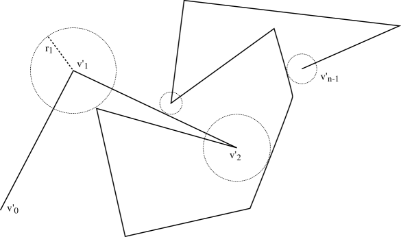
Figure 1: The projection $P^{\prime}$ of $P$. Each vertex $v^{\prime}_{i}$ is surrounded by an “empty” disk of radius $r_{i}$. Several such disks are shown.

We construct in 3D a vertical cylinder $C_{i}$ centered on each vertex $v_{i}$ of radius $r=\frac{1}{3}\min_{i}\{r_{i}\}$. This choice of $r$ ensures that no two cylinders intersect one another (the choice of the fraction $\frac{1}{3}<\frac{1}{2}$ guarantees that cylinders do not even touch), and no edges of $P$, other than those incident to $v_{i}$, intersect $C_{i}$, for all $i$.

The straightening algorithm proceeds in two stages. In the first stage, the links are squeezed like an accordion into the cylinders, so that after step $i$ all the links of $P_{i+1}=P[0,i+1]$ are packed into $C_{i+1}$. Let $\Pi_{i}$ be the vertical plane containing $e_{i}$ (and therefore $e^{\prime}_{i}$). After the first stage, the chain is monotone in $\Pi_{i}$, i.e., it is monotone with respect to the line $\Pi_{i}\cap\Pi_{xy}$ in that the intersection of the chain with a vertical line in $\Pi_{i}$ is either empty or a single point. In stage two, the chain is unraveled link by link into a straight line. The rest of this section describes the first stage. Let ${\delta}=r/n$.

2.1 Stage 1

We describe the Step 0 and the general Step $i$ separately, although the former is a special case of the latter.

1. 1. Rotate $e_{0}$ about $v_{1}$, within $\Pi_{0}$, so that the projection of $e_{0}$ on ${\Pi_{xy}}$ is contained in $e^{\prime}_{0}$ throughout the motion. The direction of rotation is determined by the relative heights ($z$-coordinates) of $v_{0}$ and $v_{1}$. Thus if $v_{0}$ is at or above $v_{1}$, $e_{0}$ is rotated upwards ($v_{0}$ remains above $v_{1}$ during the rotation); see Fig. 2. If $v_{0}$ is lower than $v_{1}$, $e_{0}$ is rotated downwards ($v_{0}$ remains below $v_{1}$ during the rotation). The rotation stops when $v_{0}$ lies within ${\delta}$ of the vertical line through $v_{1}$, i.e., when $v_{0}$ lies in the cylinder $C_{1}$ and is very close to its axis. The value of ${\delta}$ is chosen to be $r/n$ so that in later steps more links can be accommodated in the cylinder. Again see Fig. 2.

   2. Now we rotate $e_{0}$ about the axis of $C_{1}$ away from $e_{1}$, until $e^{\prime}_{0}$ and $e^{\prime}_{1}$ are collinear (but not overlapping), i.e., until $e_{0}$ lies in the vertical plane $\Pi_{1}$.

   

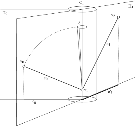
   Figure 2: Step 0: (a) $e_{0}$ is first rotated within $\Pi_{0}$ into $C_{1}$, and then (b) rotated into the vertical plane $\Pi_{1}$ containing $e_{1}$.

   After completion of Step 0, $(v_{0},v_{1},v_{2})$ forms a chain in $\Pi_{1}$ monotone with respect to the line $\Pi_{1}\cap{\Pi_{xy}}$.

2. At the start of Step $i>0$, we have a monotone chain $P_{i+1}=P[0,i+1]$ contained in the vertical plane $\Pi_{i}$ through $e_{i}$, with $P_{i}=P[0,i]$ in $C_{i}$ and $v_{0}$ within a distance of $i{\delta}$ of the axis of $C_{i}$.

   1. As in Step 0(a), rotate $e_{i}$ within $\Pi_{i}$ (in the direction that shortens the vertical projection of $e_{i}$) so that $v_{i}$ lies within a distance ${\delta}$ of the axis of $C_{i+1}$. The difference now is that $v_{i}$ is not the start of the chain, but rather is connected to the chain $P_{i}$. During the rotation of $e_{i}$ we “drag” $P_{i}$ along in such a way that only joints $v_{i}$ and $v_{i+1}$ rotate, keeping the joints $v_{1},\ldots,v_{i-1}$ frozen. Furthermore, we constrain the motion of $P_{i}$ (by appropriate rotation about joint $v_{i}$) so that it does not undergo a rotation. Thus at any instant of time during the rotation of $e_{i}$, the position of $P_{i}$ remains within $\Pi_{i}$ and is a translated copy of the initial $P_{i}$. See Fig. 3.

      

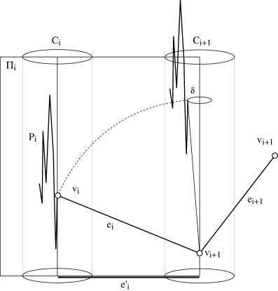
      Figure 3: The chain $P_{i}$ translates within $\Pi_{i}$.

   2. Following Step 0(b), rotate $P_{i+1}$ about the axis of $C_{i+1}$ until $e^{\prime}_{i}$ and $e^{\prime}_{i+1}$ are coplanar.

   At the completion of Step $i$ we therefore have a chain $P_{i+2}=P[0,i+2]$ in the vertical plane $\Pi_{i+1}$, with $P_{i+1}$ in $C_{i+1}$ and $v_{0}$ within a distance of $(i+1){\delta}$ of its axis. The chain is monotone in $\Pi_{i+1}$ with respect to the line $\Pi_{i+1}\cap{\Pi_{xy}}$.

2.2 Stage 2

Now it is trivial to unfold this monotone chain by straightening one joint at a time, i.e., rotating each joint angle to $\pi$, starting at either end of the chain. We have therefore established the first claim of this theorem:

Theorem 2.1

A polygonal chain of $n$ links with a simple orthogonal projection may be straightened, in $O(n)$ moves, with an algorithm of $O(n)$ time and space complexity.

Counting the number of moves is straightforward. Stage 1, Step $i$(a) requires one move: only joints $v_{i}$ and ${v_{i+1}}$ rotate. Step $i$(b) is again one move: only ${v_{i+1}}$ rotates. So Stage 1 is completed in $2n$ moves. As Stage 2 takes $n-1$ moves, the whole procedure is accomplished with $O(n)$ moves.

Each move can be computed in constant time, so the time complexity is dominated by the computation of the cylinder radii $r_{i}$. These can be trivially computed in $O(n^{2})$ time, by computing each vertex-vertex and vertex-edge distance. However, a more efficient computation is possible, based on the medial axis of a polygon, as follows. Given the projected chain $P^{\prime}$ in the plane (Fig. 4a), form two simple polygons $P_{1}$ and $P_{2}$, by doubling the chain from its endpoint $v^{\prime}_{0}$ until the convex hull is reached (say at point $x$), and from there connecting along the line bisecting the hull angle at $x$ to a large surrounding rectangle, and similarly connecting from $v^{\prime}_{n-1}$ to the hull to the rectangle. For $P_{1}$ close the polygon above $P^{\prime}$, and below for $P_{2}$. See Figs. 4bc. Note that $P_{1}\cup P_{2}$ covers the rectangle, which, if chosen large, effectively covers the plane for the purposes of distance computation.

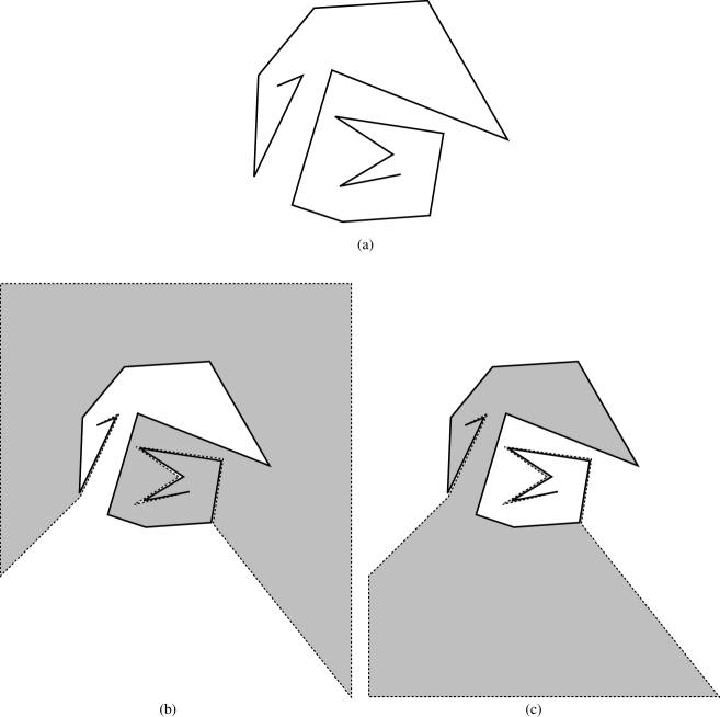
Figure 4: (a) Chain $P^{\prime}$; (b) Polygon $P_{1}$; (c) Polygon $P_{2}$.

Compute the medial axis of $P_{1}$ and $P_{2}$ using a the linear-time algorithm of [CSW95]. The distances $r_{i}$ can now be determined from the distance information in the medial axes. For a convex vertex $v_{i}$ of $P_{k}$, its minimum “feature distance” can be found from axis information at the junction of the axis edge incident to $v_{i}$. For a reflex vertex, the information is with the associated axis parabolic arc. Because the bounding box is chosen to be large, no vertex’s closest feature is part of the bounding box, and so must be part of the chain.

3 Open Chains on a Polytope

In this section we show that any open chain embedded on the surface of a convex polytope may be straightened. We start with a planar chain which we straighten in 3D.

Let $P$ be an open chain in 2D, lying in ${\Pi_{xy}}$. It may be easily straightened by the following procedure. Rotate $e_{0}$ within $\Pi_{0}$ until it is vertical; now $v_{0}$ projects into $v_{1}$ on ${\Pi_{xy}}$. In general, rotate $e_{i}$ within $\Pi_{i}$ until $v_{i}$ sits vertically above $v_{i+1}$. Throughout this motion, keep the previously straightened chain $P_{i}=P[0,i]$ above $v_{i}$ in a vertical ray through $v_{i}$. This process clearly maintains simplicity throughout, as the projection at any stage is a subset of the original simple chain in ${\Pi_{xy}}$. In fact, this procedure can be seen as a special case of the algorithm described in the preceding section.

An easy generalization of this “pick-up into a vertical ray” idea permits straightening any open chain lying on the surface of a convex polytope ${\cal P}$. The same procedure is followed, except that the surface of ${\cal P}$ plays the role of ${\Pi_{xy}}$, and surface normals play the roles of vertical rays. When a vertex $v_{i}$ of the polygonal chain $P$ lies on an edge $e$ between two faces $f_{1}$ and $f_{2}$ of ${\cal P}$, then the line containing $P_{i}$ is rotated from $R_{1}$, the ray through $v_{i}$ and normal to $f_{1}$, through an angle of measure $\pi-{\delta}(e)$, where ${\delta}(e)$ is the (interior) dihedral angle at $e$, to $R_{2}$, the ray through $v_{i}$ and normal to $f_{2}$.

This algorithm uses $O(n)$ moves and can be executed in $O(n)$ time.

Note that it is possible to draw a polygonal chain on a polytope surface that has no simple projection. So this algorithm handles some cases not covered by Theorem 2.1. We believe that the sketched algorithm applies to a class of polyhedra wider than convex polytopes, but we will not pursue this further here.

4 Locked Chains

Having established that two classes of open chains may be straightened, we show in this section that not all open chains may be straightened, describing one locked open chain of five links (Section 4.1). A modification of this example establishes the same result for closed chains (Section 4.2). Both of these results were obtained independently by other researchers [CJ98]. Our proofs are, however, sufficiently different to be of independent interest.

4.1 A Locked Open Chain

Consider the chain $K=(v_{0},\ldots,v_{5})$ configured as in Fig. 5, where the standard knot theory convention is followed to denote “over” and “under” relations. Let $L=\ell_{1}+\ell_{2}+\ell_{3}$ be the total length of the short central links, and let $\ell_{0}$ and $\ell_{4}$ be both larger than $L$; in particular, choose $\ell_{0}=L+{\delta}$ and $\ell_{4}=2L+{\delta}$ for ${\delta}>0$. (One can think of this as composed of two rigid knitting needles, $e_{0}$ and $e_{4}$, connected by a flexible cord of length $L$.) Finally, center a ball $B$ of radius $r=L+{\epsilon}$ on $v_{1}$, with $0<2{\epsilon}<{\delta}$. The two vertices $v_{0}$ and $v_{5}$ are exterior to $B$, while the other four are inside $B$. See Fig. 5.

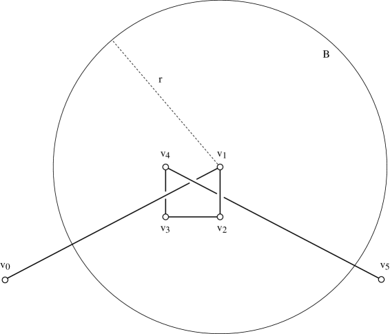
Figure 5: A locked open chain $K$ (“knitting needles”). (The first and last edges $e_{0}$ and $e_{4}$ are longer than they appear in this view.)

Assume now that the chain $K$ can be straightened by some motion. During the entire process, $\{v_{1},v_{2},v_{3},v_{4}\}\subset B$ because $L<r$. Of course $v_{0}$ remains outside of $B$ because $\ell_{0}>r$. Now because $v_{4}\in B$ and $\ell_{4}=|v_{4}v_{5}|=2L+{\delta}$ is more than the diameter $2r=2(L+{\epsilon})$ of $B$, $v_{5}$ also remains exterior to $B$ throughout the motion.

Before proceeding with the proof, we recall some terms from knot theory. The trivial knot is an unknotted closed curve homeomorphic to a circle. The trefoil knot is the simplest knot, the only knot that may be drawn with three crossings. See, e.g., [Liv93] or [Ada94].

Because of the constant separation between $\{v_{0},v_{5}\}$ and $\{v_{1},v_{2},v_{3},v_{4}\}$ by the boundary of $B$, we could have attached a sufficiently long unknotted string $P^{\prime}$ from $v_{0}$ to $v_{5}$ exterior to $B$ that would not have hindered the unfolding of $P$. But this would imply that $K\cup P^{\prime}$ is the trivial knot; but it is clearly a trefoil knot. We have reached a contradiction; therefore, $K$ cannot be straightened.

4.2 A Locked, Unknotted Closed Chain

It is easy to obtain locked closed chains in 3D: simply tie the polygonal chain into a knot. Convexifying such a chain would transform it to the trivial knot, an impossibility. More interesting for our goals is whether there exists a locked, closed polygonal chain that is unknotted, i.e., whose topologically structure is that of the trivial knot.

We achieve this by “doubling” $K$: adding vertices $v^{\prime}_{i}$ near $v_{i}$ for $i=1,2,3,4$, and connecting the whole into a chain $K^{2}=(v_{0},\ldots,v_{5},v^{\prime}_{4},\ldots,v^{\prime}_{1})$. See Fig. 6.

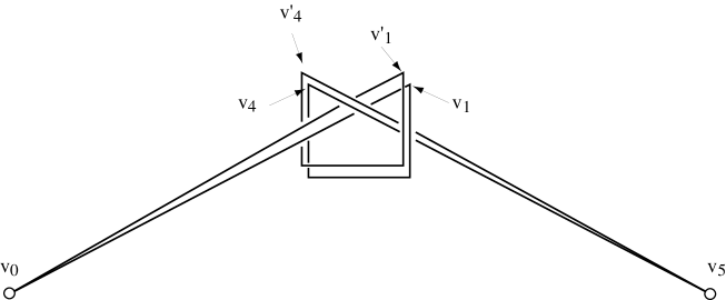
Figure 6: $K^{2}$ ($K$ doubled): a locked but unknotted chain.

Because $K\subset K^{2}$, the preceding argument applies when the second copy of $K$ is ignored: any convexifying motion will have the property that $v_{0}$ and $v_{5}$ remain exterior to $B$, and $\{v_{1},v_{2},v_{3},v_{4}\}$ remain interior to $B$ throughout the motion. Thus the extra copy of $K$ provides no additional freedom of motion to $v_{5}$ with respect to $B$. Consequently, we can argue as before: if $K^{2}$ is somehow convexified, this motion could be used to unknot $K\cup P^{\prime}$, where $P^{\prime}$ is an unknotted chain exterior to $B$ connecting $v_{0}$ to $v_{5}$. This is impossible, therefore $K^{2}$ is locked.

5 Convexifying a Planar Simple Polygon in 3D

An interesting open problem is to generalize our result from Section 2 to convexify a general closed chain. We show now that the special case of a closed chain lying in a plane, i.e., a planar simple polygon, may be convexified in 3D.

Such a polygon may be convexified in 3D by “flipping” out the reflex pockets, i.e., rotating the pocket chain into 3D and back down to the plane; see Fig. 7. This simple procedure was suggested by Erdős [Erd35] and proved to work by de Sz. Nagy [dSN39]. The number of flips, however, cannot be bound as a function of the number of vertices $n$ of the polygon, as first proved by Joss and Shannon [Grü95]. See [Tou99] for the complex history of these results.

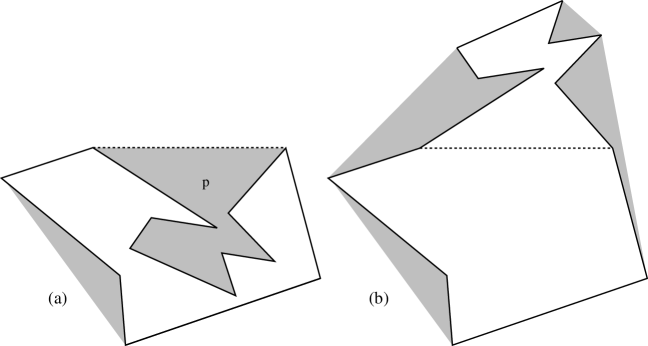
Figure 7: (a) A pocket $p$; (b) The polygon after flipping $p$.

We offer a new algorithm for convexifying planar closed chains, which we call the “St. Louis Arch” algorithm. It is more complicated than flipping but uses a bounded number of moves, in fact $O(n)$ moves. It models the intuitive approach of picking up the polygon into 3D. We discretize this to lifting vertices one by one, accumulating the attached links into a convex “arch” $A$ in a vertical plane above the remaining polygonal chain; see Fig. 8. Although the algorithm is conceptually simple, some care is required to make it precise, and to then establish that simplicity is maintained throughout the motions.

Let $P$ be a simple polygon in the $xy$-plane, ${\Pi_{xy}}$. Let ${\Pi_{\epsilon}}$ be the plane $z={\epsilon}$ parallel to ${\Pi_{xy}}$, for ${\epsilon}>0$; the value of ${\epsilon}$ will be specified later. We use this plane to convexify the arch safely above the portion of the polygon not yet picked up. We will use primes to indicate positions of moved (raised) vertices; unprimed labels refer to the original positions. After a generic step $i$ of the algorithm, $P(0,i)$ has been lifted above ${\Pi_{\epsilon}}$ and convexified, $v_{0}$ and $v_{i}$ have been raised to $v^{\prime}_{0}$ and $v^{\prime}_{i}$ on ${\Pi_{\epsilon}}$, and $P[i+1,n-1]$ remains in its original position on ${\Pi_{xy}}$. We first give a precise description of the conditions that hold after the $i$th step. Let $\Pi_{z}(v_{i},v_{j})$ be the (vertical) plane containing $v_{i}$ and $v_{j}$, parallel to the $z$-axis.

1. ${\Pi_{\epsilon}}$ splits the vertices of $P$ into three sets: $v^{\prime}_{0}$ and $v^{\prime}_{i}$ lie in ${\Pi_{\epsilon}}$, $v^{\prime}_{1},\ldots,v^{\prime}_{i-1}$ lie above the plane, and $v_{i+1},\ldots,v_{n-1}$ lie below it.

2. The arch $A=P(0,i)$ lies in the plane $\Pi_{z}(v^{\prime}_{0},v^{\prime}_{i})$, and is convex.

3. $v^{\prime}_{0}$ and $v^{\prime}_{i}$ project onto ${\Pi_{xy}}$ within distance ${\delta}$ of their original positions $v_{0}$ and $v_{i}$. (Here, $\delta>0$ is a constant that depends only on the input positions; it will be specified later.)

4. Edges ${v_{n-1}}v^{\prime}_{0}$ and $v^{\prime}_{i}{v_{i+1}}$ connect between ${\Pi_{xy}}$ and ${\Pi_{\epsilon}}$.

5. $P[i+1,n-1]$ remains in its original position in ${\Pi_{xy}}$.

See Fig. 8.

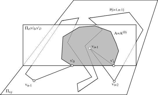
Figure 8: The arch $A$ after the $i$th step, i.e., after “picking up” $P(0,i)$ into $A$. (The planes ${\Pi_{xy}}$ and ${\Pi_{\epsilon}}$ are not distinguished in this figure, nor in Figs. 10 or 11.)

A central aspect of the algorithm will be choosing ${\epsilon}$ small enough to guarantee a ${\delta}$ (see H3) that maintains simplicity throughout all movements.

The algorithm consists of an initialization step S0, followed by repetition of steps S1–S4.

5.1 S0

The algorithm is initialized at $i=2$ by selecting an arbitrary (strictly) convex vertex $v_{1}$, and raising $\{v_{0},v_{1},v_{2}\}$ in four steps:

1. Rotate $v_{1}$ about the line through $v_{0}v_{2}$ up to ${\Pi_{\epsilon}}$. Call its new position $v^{\prime\prime}_{1}$.

2. Rotate $v_{0}$ about the line through $v_{n-1}v^{\prime\prime}_{1}$ up to ${\Pi_{\epsilon}}$. Call its new position $v^{\prime}_{0}$.

3. Rotate $v_{2}$ about the line through $v^{\prime\prime}_{1}v_{3}$ up to ${\Pi_{\epsilon}}$. Call its new position $v^{\prime}_{2}$.

4. Rotate $v^{\prime\prime}_{1}$ about the line through $v^{\prime}_{0}v^{\prime}_{2}$ upwards until it lies in the plane $\Pi_{z}(v^{\prime}_{0},v^{\prime}_{2})$. Call its new position $v^{\prime}_{1}$.

So long as the joint at $v^{\prime\prime}_{1}$ is not straight, the $4$th step above is unproblematical, simply rotating a triangle from a horizontal to a vertical plane. That this joint does not become straight depends on ${\epsilon}$ and ${\delta}$, and will be established under the discussion of S1 below. Ditto for establishing that the first three steps can be accomplished without causing self-intersection.

After completion of Step S0, the hypotheses H1–H5 are all satisfied. The remaining steps S1–S4 are repeated for each $i>2$.

5.2 S1

The purpose of Step S1 is to lift $v_{i}$ from ${\Pi_{xy}}$ to ${\Pi_{\epsilon}}$. This will be accomplished by a rotation of $v_{i}$ about the line through $v^{\prime}_{i-1}$ and $v_{i+1}$, the same rotation used in substeps (2) and (3), and in a modified form in (1), of Step S0. Although this rotation is conceptually simple, it is this key movement that demands a value of ${\epsilon}$ to guarantee a ${\delta}$ that ensures correctness. The values of ${\epsilon}$ and ${\delta}$ will be computed directly from the initial geometric structure of $P$. Specifying the conditions on ${\epsilon}$ is one of the more delicate aspects of our argument, to which we now turn.

Let ${\alpha}_{j}$ be the smaller of the two (interior and exterior) angles at $v_{j}$. Also let ${\beta}_{j}=\pi-{\alpha}_{j}$, the deviation from straightness at joint $v_{j}$. We assume that $P$ has no three consecutive collinear vertices. If a vertex is collinear with its two adjacent vertices, we freeze and eliminate that joint. So we may assume that ${\beta}_{j}>0$ for all $j$.

5.2.1 Determination of ${\delta}$

As in our earlier Figure 1, the simplicity of $P$ guarantees “empty” disks around each vertex. Here we need disks to meet more stringent conditions than used in Section 2. Let ${\delta}>0$ be such that:

1. Disks around each vertex $v_{j}$ of radius ${\delta}$ include no other vertices of $P$, and only intersect the two edges incident to $v_{j}$.

2. A perturbed polygon, obtained by displacing the vertices within the disks (ignoring the fixed link lengths),

   1. remains simple, and

   2. has no straight vertices.

It should be clear that the simplicity of $P$ together with ${\beta}_{j}>0$ guarantees that such a ${\delta}>0$ exists. As a technical aside, we sketch how ${\delta}$ could be computed. Finding a radius that satisfies condition (1) is easy. Half this radius guarantees the simplicity condition (2a), for this keeps a maximally displaced vertex separated from a maximally displaced edge. To prevent an angle ${\beta}_{j}$ from reaching zero, condition (2b), displacements of the three points $v_{j-1}$, $v_{j}$, and $v_{j+1}$ must be considered. Let $\ell=\min_{j}\{\ell_{j}\}$ be the length of the shortest edge, and let ${\beta}^{\prime}=\min_{j}\{{\beta}_{j}\}$ be the minimum deviation from collinearity. Lemma A.1,which we prove in the Appendix, shows that choosing ${\delta}<\frac{1}{2}\ell\sin({\beta}^{\prime}/2)$ prevents straight vertices.

Let ${\sigma}$ be the minimum separation $|v_{j}v_{k}|$ for all positions of $v_{j}$ and $v_{k}$ within their ${\delta}$ disks, for all $j$ and $k$. Condition (2a) guarantees that ${\sigma}>0$. Note that ${\sigma}\leq\ell$. Let ${\beta}$ be the minimum of all ${\beta}_{j}$ for all positions of $v_{j}$ within their ${\delta}$ disks. Condition (2b) guarantees that ${\beta}>0$. Our next task is to derive ${\epsilon}$ from ${\sigma}$, ${\beta}$, and ${\delta}$. To this end, we must detail the “lifting” step of the algorithm.

5.2.2 S1 Lifting

Throughout the algorithm, $v^{\prime}_{0}$ remains fixed at the position on ${\Pi_{\epsilon}}$ it reached in Step S0. During the lifting step, $v^{\prime}_{i-1}$ also remains fixed, while $v_{i}$ is lifted. Thus $v^{\prime}_{0}v^{\prime}_{i-1}$, the base of the arch $A$, remains fixed during the lifting, which permits us, by hypothesis H1, to safely ignore the arch during this step.

We now concentrate on the $2$-link chain $(v^{\prime}_{i-1},v_{i},v_{i+1})$. By H5, $v_{i}v_{i+1}$ has not moved on ${\Pi_{xy}}$; by H3, $v^{\prime}_{i-1}$ has not moved horizontally more than ${\delta}$ from $v_{i-1}$. Let ${\alpha}^{\prime}_{i}$ be the measure in $[0,\pi]$ of angle $\angle(v^{\prime}_{i-1},v_{i},v_{i+1})$, i.e., the angle at $v_{i}$ measured in the slanted plane determined by the three points. Because $v_{i}v_{i+1}$ lie on ${\Pi_{xy}}$ and $v^{\prime}_{i-1}$ is on ${\Pi_{\epsilon}}$, ${\alpha}^{\prime}_{i}\neq\pi$ and the chain $(v^{\prime}_{i-1},v_{i},v_{i+1})$ is kinked at the joint $v_{i}$.

Now imagine holding $v^{\prime}_{i-1}$ and $v_{i+1}$ fixed. Then $v_{i}$ is free to move on a circle $C$ with center on $v^{\prime}_{i-1}v_{i+1}$. See Fig. 9. This circle might lie partially below ${\Pi_{xy}}$, and is tilted from the vertical (because $v^{\prime}_{i-1}$ lies on ${\Pi_{\epsilon}}$).

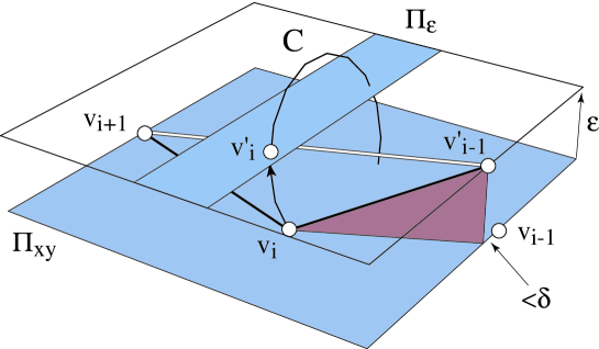
Figure 9: $v_{i}$ rotates up the circle $C$ until it hits ${\Pi_{\epsilon}}$.

The lifting step consists simply in rotating $v_{i}$ on $C$ upward until it lies on ${\Pi_{\epsilon}}$; its position there we call $v^{\prime}_{i}$.

5.2.3 Determination of ${\epsilon}$

We now choose ${\epsilon}>0$ so that two conditions are satisfied:

1. The highest point of $C$ is above ${\Pi_{\epsilon}}$ (so that $v_{i}$ can reach ${\Pi_{\epsilon}}$).

2. $v^{\prime}_{i}$ projects no more than ${\delta}$ away from $v_{i}$ (to satisfy H3).

It should be clear that both goals may be achieved by choosing ${\epsilon}$ small enough. We sketch a computation of ${\epsilon}$ in the Appendix.

The computation of ${\epsilon}$ ultimately depends solely on ${\sigma}$ and ${\beta}$—the shortest vertex separation and the smallest deviation from straightness—because these determine ${\delta}$, and then $r$ and ${\delta}_{1}$ and ${\delta}_{2}$ and ${\epsilon}$. Although we have described the computation within Step S1, in fact it is performed prior to starting any movements; and ${\epsilon}$ remains fixed throughout.

As we mentioned earlier, two of the three lifting rotations used in Step S0 match the lifting just detailed. The exception is the first lifting, of $v_{1}$ to $v^{\prime}_{1}$ in Step S0. This only differs in that the cone axis $v_{0}v_{2}$ lies on ${\Pi_{xy}}$ rather than connecting ${\Pi_{xy}}$ to ${\Pi_{\epsilon}}$. But it should be clear this only changes the above computation in that the tilt angle $\psi$ is zero, which only improves the inequalities. Thus the ${\epsilon}$ computed for the general situation already suffices for this special case.

5.2.4 Collinearity

We mention here, for reference in the following steps, that it is possible that $v^{\prime}_{i}$ might be collinear with $v^{\prime}_{0}$ and $v^{\prime}_{i-1}$ on ${\Pi_{\epsilon}}$. There are two possible orderings of these three vertices along a line:

1. $(v^{\prime}_{0},v^{\prime}_{i},v^{\prime}_{i-1})$.

2. $(v^{\prime}_{0},v^{\prime}_{i-1},v^{\prime}_{i})$.

The ordering $(v^{\prime}_{i},v^{\prime}_{0},v^{\prime}_{i-1})$ is not possible because that would violate the simplicity condition 2(a), as all three vertices project to within ${\delta}$ of their original positions on ${\Pi_{xy}}$, and no vertex comes within $\delta$ of an edge.

Despite this possible degeneracy, we will refer to “the triangle $\triangle v^{\prime}_{0}v^{\prime}_{i-1}v^{\prime}_{i}$,” with the understanding that it may be degenerate. This possibility will be dealt with in Lemma 5.6.

We now turn to the remaining three steps of the algorithm for iteration $i$. We use the notation $A^{(k)}$ to represent the arch $A=A^{(0)}$ at various stages of its processing, incrementing $k$ whenever the shape of the arch might change.

5.3 S2

After the completion of Step S1, $v^{\prime}_{i-1}v^{\prime}_{i}$ lies in ${\Pi_{\epsilon}}$. We now rotate the arch $A^{(0)}$ into the plane ${\Pi_{\epsilon}}$, rotating about its base $v^{\prime}_{0}v^{\prime}_{i-1}$, away from $v^{\prime}_{i-1}v^{\prime}_{i}$. This guarantees that $A^{(1)}=A^{(0)}\cup\triangle v^{\prime}_{0}v^{\prime}_{i-1}v^{\prime}_{i}$ is a planar weakly-simple polygon. Moreover, while $\triangle v^{\prime}_{0}v^{\prime}_{i-1}v^{\prime}_{i}$ may be degenerate, the chain $(v^{\prime}_{0},\ldots,v^{\prime}_{i})$ lies strictly to one side of the line through $(v^{\prime}_{0},v^{\prime}_{i-1})$ and so is simple. See Fig. 10.

Figure 10: $A^{(1)}=A^{(0)}\cup\triangle v^{\prime}_{0}v^{\prime}_{i-1}v^{\prime}_{i}$ lies in the plane ${\Pi_{\epsilon}}$ just slightly above ${\Pi_{xy}}$.

5.4 S3

Now that $A^{(1)}$ lies in its “own” plane ${\Pi_{\epsilon}}$, it may be convexified without worry about intersections with the remaining polygon $P[i+1,n-1]$ in ${\Pi_{xy}}$. The polygon $A^{(1)}$ is a “barbed polygon”: one that is a union of a convex polygon ($A^{(0)}$) and a triangle ($\triangle v^{\prime}_{0}v^{\prime}_{i-1}v^{\prime}_{i}$). We establish in Theorem 5.7 that $A^{(1)}$ may be convexified in such a way that neither $v^{\prime}_{0}$ nor $v^{\prime}_{i}$ move, and $v^{\prime}_{0}$ and $v^{\prime}_{i}$ end up strictly convex vertices of the resulting convex polygon $A^{(2)}$.

5.5 S4

We next rotate $A^{(2)}$ up into the vertical plane $\Pi_{z}(v^{\prime}_{0},v^{\prime}_{i})$. Because of strict convexity at $v^{\prime}_{0}$ and $v^{\prime}_{i}$, the arch stays above ${\Pi_{\epsilon}}$. See Fig. 11.

Figure 11: $A^{(2)}$, which has incorporated the edge $v_{i-1}v^{\prime}_{i}$ of $P$, is rotated up into the plane $\Pi_{z}(v^{\prime}_{0},v^{\prime}_{i})$.

We have now reestablished the induction hypothesis conditions H1–H5. After the penultimate step, for $i=n{-}2$, only $v_{n-1}$ lies on ${\Pi_{xy}}$, and the final execution of the lifting Step S1 rotates $v_{n-1}$ about $v^{\prime}_{0}v^{\prime}_{n-2}$ to raise it to ${\Pi_{\epsilon}}$. A final execution of Steps S1 and S2 yields a convex polygon. Thus, assuming Theorem 5.7 in Section 5.7 below, we have established the correctness of the algorithm:

Theorem 5.1

The “St. Louis Arch” Algorithm convexifies a planar simple polygon of $n$ vertices.

We will analyze its complexity in Section 5.8.

We now return to Step S3, convexifying a barbed polygon. We perform the convexification entirely within the plane ${\Pi_{\epsilon}}$. We found two strategies for this task. One maintains $A$ as a convex quadrilateral, and the goal of Step S3 can be achieved by convexifying the (nonconvex) pentagon $A^{(1)}$, and then reducing it to a convex quadrilateral. Although this approach is possible, we found it somewhat easier to leave $A$ as a convex $(i{+}1)$-gon, and prove that $A^{(1)}=A^{(0)}\cup\triangle v^{\prime}_{0}v^{\prime}_{i-1}v^{\prime}_{i}$ can be convexified. This is the strategy we pursue in the next two sections. Section 5.6 concentrates on the base case, convexifying a quadrilateral, and Section 5.7 achieves Theorem 5.7, the final piece needed to complete Step S3.

5.6 Convexifying Quadrilaterals

It will come as no surprise that every planar, nonconvex quadrilateral can be convexified. Indeed, recent work has shown that any star-shaped polygon may be convexified [ELR⁺98a], and this implies the result for quadrilaterals. However, because we need several variations on basic quadrilateral convexification, we choose to develop our results independently, although relegating some details to the Appendix.

Let $Q=(v_{0},v_{1},v_{2},v_{3})$ be a weakly simple, nonconvex quadrilateral, with $v_{2}$ the reflex vertex. By weakly simple we mean that either $Q$ is simple, or $v_{2}$ lies in the relative interior of one of the edges incident to $v_{0}$ (i.e., no two of $Q$’s edges properly cross). This latter violation of simplicity is permitted so that we can handle a collapsed triangle inherited from step S1 of the arch algorithm (Section 5.2.4).

As before, let ${\alpha}_{i}$ be the smaller of the two (interior and exterior) angles at $v_{i}$. Call a joint $v_{i}$ straightened if ${\alpha}_{i}=\pi$, and collapsed if ${\alpha}_{i}=0$. All motions throughout this (5.6) and the next section (5.7) are in 2D.

We will convexify $Q$ with one motion $M$, whose intuition is as follows; see Fig. 12. Think of the two links adjacent to the reflex vertex $v_{2}$ as constituting a rope. $M$ then opens the joint at $v_{0}$ until the rope becomes taut. Because the rope is shorter than the sum of the lengths of the other two links, it becomes taut prior to any other “event.”

Any motion $M$ that transforms a shape such as $Q$ can take on rather different appearances when different parts of $Q$ are fixed in the plane, providing different frames of reference for the motion. Although all such fixings represent the same intrinsic shape transformation $M$, when convenient we distinguish two fixings: $M_{02}$, which fixes the line $L$ containing $v_{0}v_{2}$, and $M_{03}$, which fixes the line containing $v_{0}v_{3}$.

The convexification motion $M$ is easiest to see when viewed as motion $M_{02}$. Here the two $2$-link chain $(v_{0},v_{1},v_{2})$ and $(v_{0},v_{3},v_{2})$ perform a line-tracking motion [LW92]: fix $v_{0}$, and move $v_{2}$ away from $v_{0}$ along the fixed directed line $L$ containing $v_{0}v_{2}$, until $v_{2}$ straightens.

Lemma 5.2

A weakly simple quadrilateral $Q$ nonconvex at $v_{2}$ may be convexified by motion $M_{02}$, which straightens the reflex joint $v_{2}$, thereby converting $Q$ to a triangle $T$. Throughout the motion, all four angles ${\alpha}_{i}$ increase only, and remain within $(0,\pi)$ until ${\alpha}_{2}=\pi$. See Fig. 12a.

Although this lemma is intuitively obvious, and implicit in work on linkages (e.g., [GN86]), we have not found an explicit statement of it in the literature, and we therefore present a proof in the Appendix (Lemma A.3).

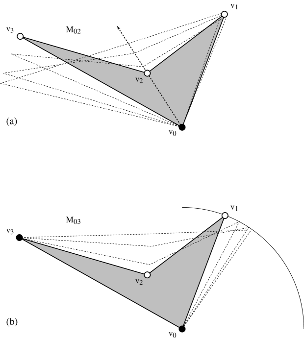
Figure 12: (a) Convexifying a quadrilateral by $M_{02}$: moving $v_{2}$ out the $v_{0}v_{2}$ diagonal; (b) The same motion viewed as $M_{03}$: opening ${\alpha}_{0}$ with $v_{0}v_{3}$ fixed.

We note that the same motion convexifies a degenerate quadrilateral, where the triangle $\triangle v_{0}v_{1}v_{2}$ has zero area with $v_{2}$ lying on the edge $v_{0}v_{1}$. See Fig. 13. As long as we open ${\alpha}_{2}$ in the direction, as illustrated, that makes the quadrilateral simple, the proof of Lemma 5.2 carries through.

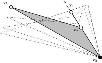
Figure 13: Motion $M_{02}$ also convexifies a weakly simple quadrilateral.

The motion $M_{02}$ used in Lemma 5.2 is equivalent to the motion $M_{03}$ obtained by fixing $v_{0}v_{3}$ and opening ${\alpha}_{0}$ by rotating $v_{1}$ clockwise (cw) around the circle of radius $\ell_{0}$ centered on $v_{0}$. Throughout this motion, the polygon stays right of the fixed edge $v_{0}v_{3}$. See Fig. 12b. This yields the following easy corollary of Lemma 5.2:

Lemma 5.3

Let $P=Q\cup P^{\prime}$ be a polygon obtained by gluing edge $v_{0}v_{3}$ of a weakly simple quadrilateral $Q$ nonconvex at $v_{2}$, to an equal-length edge of a convex polygon $P^{\prime}$, such that $Q$ and $P^{\prime}$ are on opposite sides of the diagonal $v_{0}v_{3}$. Then applying the motion $M_{03}$ to $Q$ while keeping $P^{\prime}$ fixed, maintains simplicity of $P$ throughout.

5.6.1 Strict Convexity

Motion $M$ converts a nonconvex quadrilateral into a triangle, but we will need to convert it to a strictly convex quadrilateral. This can always be achieved by continuing $M_{02}$ beyond the straightening of ${\alpha}_{2}$.

Lemma 5.4

Let $Q=(v_{0},v_{1},v_{2},v_{3})$ be a quadrilateral, with $(v_{1},v_{2},v_{3})$ collinear so that ${\alpha}_{2}=\pi$, and such that $\triangle v_{0}v_{1}v_{3}$ is nondegenerate. As in Lemma 5.3, let $P=Q\cup P^{\prime}$ be a convex polygon obtained by gluing $P^{\prime}$ to edge $v_{0}v_{3}$ of $Q$, with $v_{0}$ and $v_{3}$ strictly convex vertices of $P$. The motion $M_{02}$ (moving $v_{2}$ along the line determined by $v_{0}v_{2}$) transforms $Q$ to a strictly convex quadrilateral $Q^{\prime}$ such that $Q^{\prime}\cup P^{\prime}$ remains a convex polygon (See Fig. 14.)

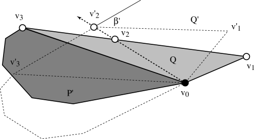
Figure 14: Converting $Q$ to the strictly convex quadrilateral $Q^{\prime}$ via $M_{02}$. Attachment $P^{\prime}$ is carried along rigidly.

Proof: Because $v_{0}$ and $v_{3}$ are strictly convex vertices, and $v_{1}$ must be strictly convex because $Q$ is a nondegenerate triangle, all the interior angles at these vertices are bounded away from $\pi$. By assumption, they are also bounded away from $0$. Thus there is some freedom of motion for $v_{2}$ along the line determined by $v_{0}v_{2}$ before the next event, when one of these angles reaches $0$ or $\pi$. $\Box$

A lower bound on ${\beta}^{\prime}=\pi-{\alpha}^{\prime}_{2}$, the amount that $v_{2}$ can be bent before an event is reached, could be computed explicitly in $O(1)$ time from the local geometry of $Q\cup P^{\prime}$, but we will not do so here.

5.7 Convexifying Barbed Polygons

Call a polygon barbed if removal of one ear $\triangle abc$ leaves a convex polygon $P^{\prime}$. $\triangle abc$ is called the barb of $P$. Note that either or both of vertices $a$ and $c$ may be reflex vertices of $P$. In order to permit $\triangle abc$ to be degenerate (of zero area), we extend the definition as follows. A weakly simple polygon (Section 5.6, Figure 13) is barbed if, for three consecutive vertices $a$, $b$, $c$, deletion of $b$ (i.e., removal of the possibly degenerate $\triangle abc$) leaves a simple convex polygon $P^{\prime}$. Note this definition only permits weak simplicity at the barb $\triangle abc$.

The following lemma (for simple barbed polygons) is implicit in [Sal73], and explicit (for star-shaped polygons, which includes barbed polygons) in [ELR⁺98b], but we will need to subsequently extend it, so we provide our own proof.

Lemma 5.5

A weakly simple barbed polygon may be convexified, with $O(n)$ moves.

Proof: Let $P=(v_{0},v_{1},\ldots,v_{n-1})$, with $\triangle v_{0}v_{n-2}v_{n-1}$ the barb. See Fig. 15.

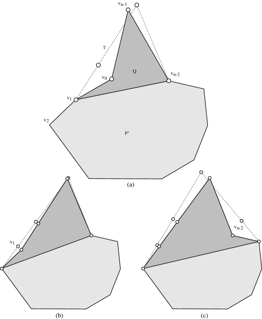
Figure 15: (a) A barbed polygon with barb $\triangle v_{0}v_{n-2}v_{n-1}$. The nonconvex quadrilateral $Q$ is transformed to $T$, resulting in a new barbed polygon $T\cup P^{\prime\prime}$. (b) and (c) show the remaining convexification steps.

The proof is by induction. Lemma 5.2 establishes the base case, $n=4$, for every quadrilateral is a barbed polygon. So assume the theorem holds for all barbed polygons of up to $n-1$ vertices.

If both $v_{0}$ and $v_{n-2}$ are convex, $P$ is already convex and we are finished. So assume that $P$ is nonconvex, and without loss of generality let $v_{0}$ be reflex in $P$. It must be that $v_{1}v_{n-2}$ is a diagonal, as it lies within the convex portion of $P$. Let $Q=(v_{0},v_{1},v_{n-2},v_{n-1})$ be the quadrilateral cut off by diagonal $v_{1}v_{n-2}$, and let $P^{\prime\prime}=(v_{1},\ldots,v_{n-2})$ be the remaining portion of $P$, so that $P=Q\cup P^{\prime\prime}$. $Q$ is nonconvex at $v_{0}$.

Lemma 5.3 shows that motion $M$ (appropriately relabeled) may be applied to convert $Q$ to a triangle $T$ by straightening $v_{0}$, leaving $P^{\prime\prime}$ unaffected. At the end of this motion, we have reduced $P$ to a polygon $P^{\prime}$ of one fewer vertex. Now note that $T$ is a barb for $P^{\prime}$ (because $P^{\prime\prime}$ is convex): $P^{\prime}=T\cup P^{\prime\prime}$. Apply the induction hypothesis to $P^{\prime}$. The result is a convexification of $P$.

Each reduction uses one move $M$, and so $O(n)$ moves suffice for $P$. $\Box$

Note that although each step of the convexification straightens one reflex vertex, it may also introduce a reflexivity: $v_{1}$ is convex in Fig. 15a but reflex in Fig. 15b. We could make the procedure more efficient by “freezing” any joint as soon as it straightens, but it suffices for our analysis to freeze each straightened reflex vertex, thenceforth treating the segment on which it lies as a single rigid link.

As is evident in Fig. 15c, the convexification leaves a polygon with several vertices straightened. One of the edges $e$ of the barbed polygon is the base of the arch $A$ from Section 5.2.2. If either of $e$’s endpoints are straightened, then part of the arch will lie directly in the plane ${\Pi_{\epsilon}}$, and could cause a simplicity violation during the S1 lifting step. Therefore we must ensure that both of $e$’s endpoints are strictly convex:

Lemma 5.6

Any convex polygon with a distinguished edge $e$ can be reconfigured so that that both endpoints of $e$ become strictly convex vertices.

Proof: Suppose the counterclockwise endpoint $v_{2}$ of $e$ has internal angle ${\alpha}=\pi$; see Fig. 16. Let $v_{1}$ be the next strictly convex vertex in clockwise order before $v_{2}$ (it may be that $v_{1}$ is the other endpoint of $e$), and $v_{3},v_{0}$ be the next two strictly convex vertices adjacent to $v_{2}$ counterclockwise. Let $Q=(v_{0},v_{1},v_{2},v_{3})$.

Figure 16: Making one endpoint of $e$ strictly convex.

Then apply Lemma 5.4 to $Q$ to convexify $v_{2}$ via motion $M_{02}$. Apply the same procedure to the other endpoint of $e$ if necessary. $\Box$

Using Lemma 5.5 to convexify the barbed polygon arch, and Lemma 5.6 to make its base endpoints strictly convex, yields:

Theorem 5.7

A weakly simple barbed polygon may be convexified in such a way that the endpoints of a distinguished edge are strictly convex.

This completes the description of the St. Louis Arch Algorithm, as $A^{(1)}=A^{(0)}\cup\triangle v^{\prime}_{0}v^{\prime}_{i-1}v^{\prime}_{i}$ is a barbed polygon, and Step S4 may proceed because of the strict convexity at the arch base endpoints.

5.8 Complexity of St. Louis Arch Algorithm

It is not difficult to see that only a constant number of moves are used in steps S0, S1, S2, and S4. Step S3 is the only exception, which we have seen in Lemma 5.5 can be executed in $O(n)$ moves. So the resulting procedure can be accomplished in $O(n^{2})$ moves. The algorithm actually only uses $O(n)$ moves, as the following amortization argument shows:

Lemma 5.8

The St. Louis Arch Algorithm runs in $O(n)$ time and uses $O(n)$ moves.

Proof: Each barb convexification move used in the proof of Lemma 5.5 constitutes a single move according to the definition in Section 1.2, as four joints open monotonically (cf. Lemma 5.2). Each such convexification move necessarily straightens one reflex joint, which is subsequently “frozen.” The number of such freezings is at most $n$ over the life of the algorithm. So although any one barbed polygon might require $\Omega(n)$ moves to convexify, the convexifications over all $n$ steps of the algorithm uses only $O(n)$ moves. Making the base endpoint angles strictly convex requires at most two moves per step, again $O(n)$ overall.

Each step of the algorithm can be executed in constant time, leading to a time complexity of $O(n)$. Again we must consider computation of the minimum distances around each vertex to obtain ${\delta}$ (Section 5.2.1), but we can employ the same medial axis technique used in Section 2 to compute these distances in $O(n)$ time. $\Box$

Note that at most four joints rotate at any one time, in the barb convexification step.

6 Open problems

Although we have mapped out some basic distinctions between locked and unlocked chains in three dimensions, our results leave many aspects unresolved:

1. What is the complexity of deciding whether a chain in 3D can be unfolded?

2. Theorem 2.1 only covers chains with simple orthogonal projections. Extension to perspective (central) projections, or other types of projection, seems possible.

3. Can a closed chain with a simple projection always be convexified? None of the algorithms presented in this paper seem to settle this case.

4. Find unfolding algorithms that minimize the number of simultaneous joint rotations. Our quadrilateral convexification procedure, for example, moves four joints at once, whereas pocket flipping moves only two at once.

5. Can an open chain of unit-length links lock in 3D? Cantarella and Johnson show in [CJ98] that the answer is no if $n\leq 5$.

Acknowledgements

We thank W. Lenhart for co-suggesting the knitting needles example in Fig. 5, J. Erickson for the amortization argument that reduced the time complexity in Lemma 5.8 to $O(n)$, and H. Everett for useful comments.

Appendix A Appendix

A.1 Computation of $\epsilon$

Here we detail a possible computation of $\epsilon$, as needed in Section 5.2.3.

The smallest radius $r$ for the circle $C$ is determined by the minimum angle ${\beta}$ (the smallest deviation from straightness) and the shortest edge length $\ell$. In particular, $r\geq\ell\sin({\beta}/2)$; see Figure 17a,b. Here it is safe to use the ${\beta}$ from the plane ${\Pi_{xy}}$ because the deviation from straightness is only larger in the tilted plane of $\triangle v_{i+1},v_{i},v^{\prime}_{i-1}$ (cf. Fig. 9), and we seek a lower bound on $r$.

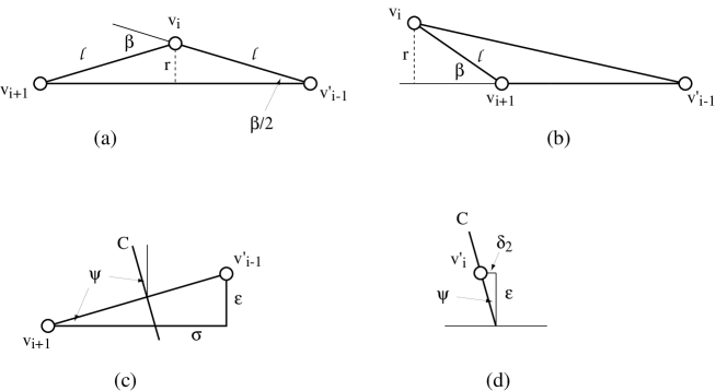
Figure 17: Determination of smallest circle radius $r$: (a) $r\geq\ell\sin({\beta}/2)$; (b) $r\geq\ell\sin{\beta}$. So $\ell\sin({\beta}/2)$ is a lower bound. Determination of largest circle tilt $\psi$: (c) $\cos\psi\geq{\sigma}/\sqrt{{\sigma}^{2}+{\epsilon}^{2}}$. (d) Determination of ${\delta}_{2}$: ${\delta}_{2}\leq{\epsilon}\tan\psi$.

The tilt $\psi$ of the circle leaves the top of $C$ at least at height $r\cos\psi$. Because $|v^{\prime}_{i-1}v_{i+1}|\geq{\sigma}$, the tilt angle must satisfy $\cos\psi\geq{\sigma}/\sqrt{{\sigma}^{2}+{\epsilon}^{2}}$; see Figure 17c. Thus to meet condition (1), we should arrange that

$$\ell\sin({\beta}/2){\frac{{\sigma}}{\sqrt{{\sigma}^{2}+{\epsilon}^{2}}}}>{\epsilon}$$

which can clearly be achieved by choosing ${\epsilon}$ small enough, as $\ell$, ${\beta}$, and ${\sigma}$ are all constants fixed by the geometry of $P$.

Turning to condition (2) of Section 5.2.3, the movement of $v^{\prime}_{i}$ with respect to $v_{i}$ can be decomposed into two components. The first is determined by the rotation along $C$ if that circle were vertical. This deviation is no more than ${\delta}_{1}=r(1-\cos\phi)$, where $\phi$ is the lifting rotation angle measured at the cone axis $v^{\prime}_{i-1}v_{i+1}$. Because $\sin\phi\leq{\epsilon}/r$, this leads to ${\delta}_{1}\leq r\left[1-\sqrt{1-({\epsilon}/r)^{2}}\right]$. The second component is due to the tilt of the circle, which is ${\delta}_{2}={\epsilon}\tan\psi\leq{\epsilon}^{2}/{\sigma}$; see Figure 17d. The total displacement is no more than ${\delta}_{1}+{\delta}_{2}$. Now it is clear that as ${\epsilon}\rightarrow 0$, both ${\delta}_{1}\rightarrow 0$ and ${\delta}_{2}\rightarrow 0$. Thus for any given ${\delta}$, we may choose ${\epsilon}$ such that ${\delta}_{1}+{\delta}_{2}<{\delta}$.

A.2 Straightening Lemma

The following lemma is used to determine ${\delta}$ in Section 5.2.1.

Lemma A.1

Let $ABC$ be a triangle, with $|AB|\geq\ell$, $|BC|\geq\ell$, and ${\beta}\leq\angle ABC\leq\pi-{\beta}$. Then for any triangle $A^{\prime}B^{\prime}C^{\prime}$ whose vertices are displaced at most ${\delta}$ from those of $\triangle ABC$, i.e.,

$$|AA^{\prime}|\><\>{\delta},\;\;|BB^{\prime}|\><\>{\delta},\;\;|CC^{\prime}|\><\>{\delta},$$

$\angle A^{\prime}B^{\prime}C^{\prime}<\pi$.

Proof: Let $a$ be the point on $BA$ a distance $\ell/2$ from $B$, and let $c$ be the point on $BC$ a distance $\ell/2$ from $B$. Let $L$ be the line containing $ac$. Set ${\theta}=\angle Bac=\angle acB$, and $\phi=\angle aBc=\pi-2{\theta}$. Because $\phi=\angle ABC$, the assumptions of the lemma give ${\beta}\leq\pi-2{\theta}\leq\pi-{\beta}$, or ${\beta}/2\leq{\theta}\leq(\pi-{\beta})/2$. The distance $d(A,L)$ from $A$ to $L$ satisfies

$$d(A,L) \geq (\ell/2)\sin{\theta}$$ (1)

$$\geq (\ell/2)\sin({\beta}/2)$$ (2)

$$> {\delta}\;.$$ (3)

The exact same inequality hold for the distances $d(B,L)$ and $d(C,L)$, because the relevant angle is ${\theta}$ is each case, and the relevant hypotenuse is $\geq\ell/2$ in each case.

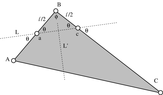
Figure 18: $A$ and $C$ are separated by $L$ from $B$, and by $L^{\prime}$ from each other.

Now suppose the three vertices $A^{\prime}$, $B^{\prime}$, $C^{\prime}$ each move no more than ${\delta}$ from $A$, $B$, and $C$ respectively. Then $L$ continues to separate $A^{\prime}$ and $C^{\prime}$ from $B^{\prime}$, by the above argument.

$\Box$

A.3 Quadrilateral Convexification

The next results are employed in Section 5.6 on convexifying quadrilaterals. We need the following lemma that states that the reflex joint of a quadrilateral can be straightened in the first place. Let $Q=v_{0}v_{1}v_{2}v_{3}$ be a four-bar linkage with $v_{2}$ a reflex joint.

Lemma A.2

A non-convex four-bar linkage can be convexified into a triangle by straightening its reflex joint.

Proof: Let $ray(v_{0},v_{2})$ be the ray starting at $v_{0}$ in the direction of $v_{2}$ and refer to Figure 19. Without loss of generality let $v_{0}$ be the origin, $ray(v_{0},v_{2})$ the positive $x$-axis and assume the sum of the link lengths $(l_{0}+l_{1})$ is smaller than $(l_{2}+l_{3})$. Assume that $v_{2}$ is translated continuously along the $x$-axis in the positive direction until it gets stuck. Since $v_{2}$ cannot move further it follows that joints $v_{0}$, $v_{1}$ and $v_{2}$ all lie on the $x$-axis and joint $v_{1}$ has been straightened. This implies the new interior angle of $v_{2}$, $\gamma<\pi$. But before the motion $v_{2}$ was a reflex angle with $\gamma>\pi$. Since the angles change continuously there must exist a point during the motion at which $\gamma=\pi$. $\Box$

Lemma A.3

When $d(v_{0},v_{2})$ is increased, all joints of the linkage open, that is, the interior angles of the convex joints and the exterior angle of the reflex joint all increase.

Proof: We will show that if $v_{2}$ is moved along $ray(v_{0},v_{2})$ in such a way that the distance $d(v_{0},v_{2})$ is increased by some positive real number $\epsilon$, no matter how small, while $v_{2}$ remains reflex, then all joints open. First note that by Euclid’s Proposition 24 of Book I, $v_{1}$ and $v_{3}$ open, that is, their interior angles increase. Secondly, note that if the interior angle at $v_{0}$ opens then so does the exterior angle at $v_{2}$ (and vice-versa) by applying Euclid’s Proposition 24 to distance $d(v_{1},v_{3})$. Hence another way to state the theorem in terms of distances only is: in a non-convex four-bar linkage the length of the interior diagonal increases if, and only if, the length of the exterior diagonal increases. It remains to show that increasing $d(v_{0},v_{2})$ increases the angle at $v_{0}$.

Before proceeding let us take care of the value of $\epsilon$. While there is no problem selecting $\epsilon$ too small, we must ensure it is not too big, for otherwise when we increase $d(v_{0},v_{2})$ by $\epsilon$ the linkage may become convex. From Lemma A.2 we know that as $d(v_{0},v_{2})$ is increased the linkage will become a triangle at some point when joint $v_{2}$ straightens, at which time $d(v_{0},v_{2})$ will have reached its maximum value, say $l$. Using the law of cosines for this triangle we obtain

$$l^{2}=l^{2}_{2}+l^{2}_{3}-l_{2}\{[(l_{1}+l_{2})^{2}+l^{2}_{3}-l^{2}_{0}]/(l_{1}+l_{2})\}.$$

Therefore if we choose $\epsilon$ such that

$$\epsilon<l-d(v_{0},v_{2}),$$

then we ensure that $v_{2}$ remains reflex.

It is convenient to analyse the situation with link $v_{3}v_{0}$ as a rigid frame of reference rather than the $ray(v_{0},v_{2})$. Therefore let both $v_{0}$ and $v_{3}$ be fixed in the plane. Then as $d(v_{0},v_{2})$ increases, from Euclid’s Proposition 24 it follows that $v_{1}$ rotates about $v_{0}$ along the fixed circle $C(v_{0},l_{0})$ centered at $v_{0}$ of radius $l_{0}$, $v_{2}$ rotates about $v_{3}$ on the fixed circle $C(v_{3},l_{2})$ centered at $v_{3}$ with radius $l_{2}$, and $ray(v_{0},v_{2})$ rotates about $v_{0}$.

Denote the initial configuration by $Q=v_{0}v_{1}v_{2}v_{3}$ and the final configuration after $d(v_{0},v_{2})$ is increased by $\epsilon$ by $Q^{\prime}=v_{0}u_{1}u_{2}v_{3}$. In other words $v_{1}$ has moved to $u_{1}$, $v_{2}$ has moved to $u_{2}$ and $ray(v_{0},v_{2})$ has moved to $ray(v_{0},u_{2})$. Since the exterior angle at $v_{2}$ is less than $\pi$ and link $v_{3}v_{2}$ rotates in a counterclockwise manner this motion causes $u_{2}$ to penetrate the interior of the shaded circle $C(v_{1},l_{1})$ centered at $v_{1}$ with radius $l_{1}$. Furthermore, $u_{2}$ cannot overshoot this shaded circle and find itself in its exterior after having penetrated it, for this would imply the joint $u_{2}$ is convex, which is impossible for the value of $\epsilon$ we have chosen. Now, since $u_{2}$ is in the interior of the shaded disk $C(v_{1},l_{1})$ and the radius of this disk is $l_{1}$ it follows that the distance $d(u_{2},v_{1})$ is less than the link length $l_{1}$. Let us therefore extend the segment $u_{2}v_{1}$ along the $ray(u_{2},v_{1})$ to a point $u^{\prime}_{2}$ so that $d(u_{2},u^{\prime}_{2})=l_{1}$. Note that the figure shows the situation when $u_{2}^{\prime}$ lies in the exterior of $C(v_{0},l_{0})$. If $u_{2}^{\prime}$ lies on $C(v_{0},l_{0})$ it yields $u_{1}$ imediately. If $u_{2}^{\prime}$ lies in the interior of $C(v_{0},l_{0})$ then the arc $u_{1},u_{2}^{\prime},u_{1}^{\prime}$ in the figure would be in the interior of $C(v_{0},l_{0})$. But of course $u_{1}$, the new position of $v_{1}$, must lie on the circle $C(v_{0},l_{0})$. To compute the possible locations for $u_{1}$ we rotate segment $u_{2}u^{\prime}_{2}$ about $u_{2}$ in both the clockwise and counterclockwise directions to intersect the circle $C(v_{0},l_{0})$ at points $u_{1}$ and $u^{\prime}_{1}$, respectively. Since $u_{2}$ lies on $ray(v_{0},u_{2})$ it follows that $u^{\prime}_{1}$ lies to the left of $ray(v_{0},u_{2})$. But the two links $v_{0}u_{1}$ and $u_{1}u_{2}$ must remain to the right of $ray(v_{0},u_{2})$ because the links are not allowed to cross each other. Therefore $u^{\prime}_{1}$ cannot be the final position of link $v_{1}$ and the latter must move to $u_{1}$. Now since

$$d(u_{2},u^{\prime}_{2})=l_{1}>d(u_{2},v_{1}),$$

it follows that $u_{1}$ lies clockwise from $v_{1}$. Therefore link $v_{0}v_{1}$ has rotated clockwise with respect to $v_{0}$ and since link $v_{0}v_{3}$ is fixed the interior angle at $v_{0}$ has increased, proving the theorem. $\Box$

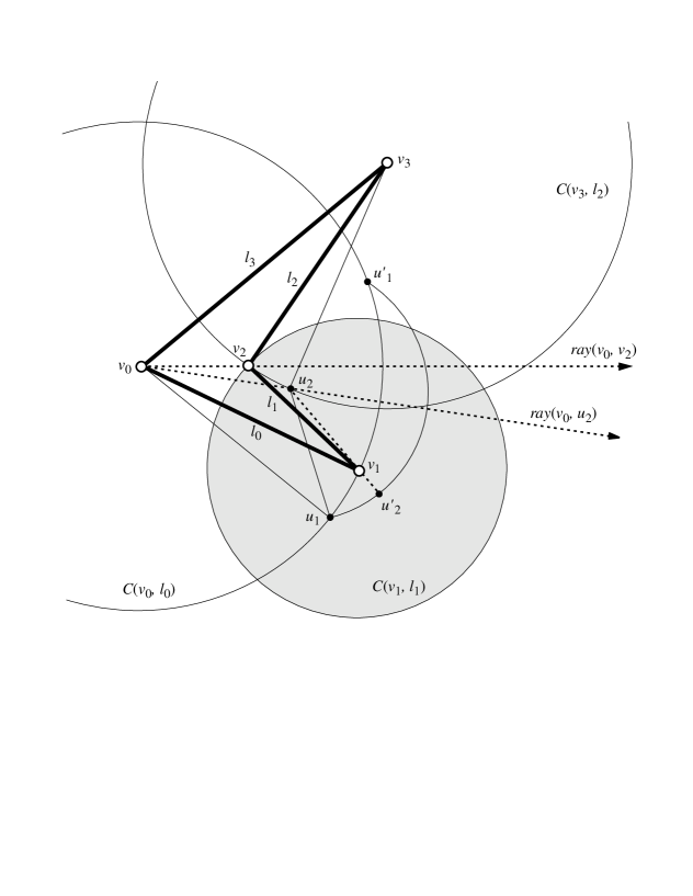
Figure 19: Line tracking holding link $v_{0}v_{3}$ fixed.

References

- [Ada94] C. C. Adams. The Knot Book. W. H. Freeman, New York, 1994.
- [BDD+99] T. Biedl, E. Demaine, M. Demaine, S. Lazard, A. Lubiw, J. O’Rourke, M. Overmars, S. Robbins, I. Streinu, G. Toussaint, and S. Whitesides. Locked and unlocked polygonal chains in 3D. In Proc. 10th ACM-SIAM Sympos. Discrete Algorithms, pages 866–867, January 1999.
- [BGRT96] P. Bose, F. Gomez, P. Ramos, and G. T. Toussaint. Drawing nice projections of objects in space. In Graph Drawing (Proc. GD ’95), volume 1027 of Lecture Notes Comput. Sci., pages 52–63. Springer-Verlag, 1996.
- [Can87] J. Canny. The Complexity of Robot Motion Planning. ACM – MIT Press Doctoral Dissertation Award Series. MIT Press, Cambridge, MA, 1987.
- [CH88] G. Crippen and T. Havel. Distance Geometry and Molecular Conformation. Research Studies Press, Letchworth, UK, 1988.
- [CJ98] J. Cantarella and H. Johnston. Nontrivial embeddings of polygonal intervals and unknots in 3-space. J. Knot Theory Ramifications, 7:1027–1039, 1998.
- [CO99] R. Cocan and J. O’Rourke. Polygonal chains cannot lock in 4d. In Proc. 11th Canad. Conf. Comput. Geom., 1999. Extended abstract. Full version: LANL/CoRR paper cs.CG/9908005.
- [Cro97] P. Cromwell. Polyhedra. Cambridge University Press, 1997.
- [CSW95] F. Chin, J. Snoeyink, and C.-A. Wang. Finding the medial axis of a simple polygon in linear time. In Proc. 6th Annu. Internat. Sympos. Algorithms Comput., volume 1004 of Lecture Notes Comput. Sci., pages 382–391. Springer-Verlag, 1995.
- [dSN39] B. de Sz. Nagy. Solution to problem 3763. Amer. Math. Monthly, 46:176–177, 1939.
- [ELR+98a] H. Everett, S. Lazard, S. Robbins, H. Schröder, and S. Whitesides. Convexifying star-shaped polygons. In Proc. 10th Canad. Conf. Comput. Geom., 1998.
- [ELR+98b] H. Everett, S. Lazard, S. Robbins, H. Schröder, and S. Whitesides. Convexifying star-shaped polygons. In Proc. 10th Canad. Conf. Comput. Geom., pages 2–3, 1998.
- [Erd35] P. Erdős. Problem 3763. Amer. Math. Monthly, 42:627, 1935.
- [GN86] C. C. Gibson and P. E. Newstead. On the geometry of the planar 4-bar mechanism. Acta Applicandae Mathematicae, 7:113–135, 1986.
- [Grü95] B. Grünbaum. How to convexify a polygon. Geombinatorics, 5:24–30, July 1995.
- [HJW84] J. E. Hopcroft, D. A. Joseph, and S. H. Whitesides. Movement problems for -dimensional linkages. SIAM J. Comput., 13:610–629, 1984.
- [Hun78] K. H. Hunt. Kinematic geometry of mechanisms. Oxford University Press, 1978.
- [Kan97] V. Kantabutra. Reaching a point with an unanchored robot arm in a square. Internat. J. Comput. Geom., 7(6):539–550, 1997.
- [Kor85] J. U. Korein. A Geometric Investigation of Reach. ACM distinguished disserations series. MIT Press, 1985.
- [Liv93] C. Livingston. Knot Theory. The Mathematical Association of America, 1993.
- [LW92] W. J. Lenhart and S. H. Whitesides. Reconfiguration with line tracking motions. In Proc. 4th Canad. Conf. Comput. Geom., pages 198–203, 1992.
- [LW95] W. J. Lenhart and S. H. Whitesides. Reconfiguring closed polygonal chains in Euclidean -space. Discrete Comput. Geom., 13:123–140, 1995.
- [Sal73] G. T. Sallee. Stretching chords of space curves. Geometriae Dedicata, 2:311–315, 1973.
- [SS83] J. T. Schwartz and Micha Sharir. On the “piano movers” problem II: General techniques for computing topological properties of real algebraic manifolds. Adv. Appl. Math., 4:298–351, 1983.
- [Tou99] G. T. Toussaint. The Erdős-Nagy theorem and its ramifications. In Proc. 11th Canad. Conf. Comput. Geom., 1999. Extended abstract.
- [vKSW96] M. van Kreveld, J. Snoeyink, and S. Whitesides. Folding rulers inside triangles. Discrete Comput. Geom., 15:265–285, 1996.
- [Whi92] S. H. Whitesides. Algorithmic issues in the geometry of planar linkage movement. Australian Comput. J., pages 42–50, 1992.
- [Whi97] W. Whiteley. Rigidity and scene analysis. In Jacob E. Goodman and Joseph O’Rourke, editors, Handbook of Discrete and Computational Geometry, chapter 49, pages 893–916. CRC Press LLC, Boca Raton, FL, 1997.