Geometric compression for progressive transmission

Abstract

The compression of geometric structures is a relatively new field of data compression. Since about 1995, several articles have dealt with the coding of meshes, using for most of them the following approach: the vertices of the mesh are coded in an order such that it contains partially the topology of the mesh. In the same time, some simple rules attempt to predict the position of the current vertex from the positions of its neighbours that have been previously coded.
In this article, we describe a compression algorithm whose principle is completely different: the order of the vertices is used to compress their coordinates, and then the topology of the mesh is reconstructed from the vertices. This algorithm, particularly suited for terrain models, achieves compression factors that are slightly greater than those of the currently available algorithms, and moreover, it allows progressive and interactive transmission of the meshes.
Keywords: geometry, compression, coding, triangulation, mesh, reconstruction, terrain models, GIS

1 Introduction

1.1 Motivations

In the context of image visualization in a network application, a remote server has to transmit data to a client. These data are usually bitmaps data and are transfered through some compression algorithm. This method has also been used in the past for computer graphics images, but in that special case, another solution consists in transmitting the scene description and in running the image synthesis program on the client. A 3D geometric scene is made of polygons, and so is typically coded as a sequence of numbers (the vertices coordinates) and tuples of vertices pointers (the edges joining the vertices).
If the problem of bitmap image compression has already been widely studied, the compression of geometric data, lying between computational geometry and data compression, is quite a new field of research.

Yet the rapid growth of image synthesis applications make necessary the manipulation and the exchange of this type of data in a fast and economical manner. In particular, the numerous possibilities given by the World Wide Web in the field of virtual reality could be dramatically restricted whithout a fast access to the data. This implies — especially for remote access through low bandwidth lines — that the geometrical data would be efficiently structured.

1.2 Related works

Among the few works about the compression of meshes ($2$ or $3$-dimensional geometric scenes made of polygons), two articles have hold our attention, for historical and efficiency reasons.

Geometric Compression Through Topological Surgery, by Taubin and Rossignac [10] describes one of the first algorithms that use the transmission order of the mesh vertices to code the topology, then that codes the vertices positions efficiently by applying prediction rules. This algorithm — that handles triangle meshes only — decomposes the mesh in triangle strips, and codes the vertices in their order of appearance in the strips, which amounts to code the connectivity of the triangulation. On the other hand, since this order preserves the geometrical neighbourhood of the vertices, it allows to linearly predict the position of a vertex from the positions of vertices immediatly preceeding in the code. So, instead of coding the absolute coordinates of each vertex, the algorithm uses standard entropy coding methods to send only the error resulting from the predictive technique.
Compared to the other methods based on the decomposition of the triangle mesh into triangle strips (in particular, those of Deering [5] and Chow [4]), this one seems to give the best compression factor on practical examples.

Triangle Mesh Compression, by Touma and Gotsman [11] describes another algorithm, whose general principle is quite close. The first difference is the way to traverse the triangulation. The algorithm maintains a list of vertices (initialized with one arbitrary mesh vertex) forming a polygon which contains all the coded triangles. The polygon grows by inserting the polygonal line that joins the vertices adjacent to a given polygon vertex and outside the polygon. This gives an order over the vertices of the mesh which allows to reconstruct its topology with few additional information. The second difference with the previous algorithm is the method used to predict a vertex position from its predecessors in the code. Besides a linear prediction technique, the algorithm estimates the crease between the current triangles from the previous creases. This yields better compression factors in practice.

These two algorithms are designed for triangular surfaces in the 3-dimensional space. The case of genus greater than $0$ is deduced from the null genus case by adding some artificial data. It is also important to note that these algorithms first quantize the vertices coordinates to a number of bits typically lying between $8$ and $12$. The predictive techniques apply to these quantized positions.

1.3 Framework

In this article, we tackle the problem of coding geometrical structures in a different way. We use the fact that in many cases, the 3D objects are constructed automatically from points samples. Hence the topology of a mesh can often be reconstructed from its vertices.
Consequently, our algorithm exploits the transmission order of the vertices to code only their coordinates. So it can be applied to any geometric structure as long as a reconstruction algorithm is available for the topology of the original object.

An example of automatic construction of a mesh from its vertices is given by the Delaunay triangulation. In dimension $2$, it is a triangulation that offers some useful properties, like to maximize the smallest angle of the triangulation, that is to say to create regular triangles. The Delaunay triangulation has also applications in the field of 3D scenes, in particular with the terrain models, whose topology is generally obtained by triangulating the points without their z-coordinates.

The efficient transmission of the Delaunay triangulation of a set of 2D points is a common problem in GIS (geographic information systems), handled by Snoeyink and van Kreveld [8], and more recently Sohler [9]. However, in these works, the purpose is quite different of ours: the transmission order over the points is used to speed up the reconstruction of the triangulation (a linear time is obtained, instead of $n\,\log n$). In addition, some compression is achieved by coding differentially the vertices coordinates with variable length codes. However, that does not constitute the main concern of these methods, and the compression factors achieved are relatively low.

2 Description of the algorithm

In order to simplify the description of the algorithm, we start by handling the dimension 1 case. We will see that the generalization to any dimension is straightforward.

We first describe the coding part of the algorithm. Let $S$ be a set of $n$ points lying on a line segment, between $0$ and $2^{b}$ (so the coordinates of the points are coded on $b$ bits). The algorithm begins to code the total number of points on an arbitrary fixed number of bits ($32$ for example). Then it starts up the main loop which consists in subdividing the current segment in two halfs and in coding the number of points contained in one of them (the left half-segment for exemple) on an optimal number of bits: if the current segment contains $p$ points, the number of points in the half-segment will be coded on $\log_{2}(p+1)$ bits. We will see in Section 5 how it is possible to code a symbol on a non integer number of bits.
So the algorithm maintains a list of segments composed of:

• the length of the segment,

• the position of the segment,

• a list of the points lying on the segment.

Each segment is removed from the list, subdivided in $2$ half-segments inserted at the end of the list if they contain points, and give birth to an output code corresponding to the number of points in the left half-segment. The algorithm stops when there are no more divisible segments in the current list, that is to say no segment of length greater than $1$. The pseudo-code below details the functioning of the coding part.

• ${\cal L}$ $\mathrel{\leftarrow}$original line segment ${\cal S}_{0}$

• output the number of points on ${\cal S}_{0}$ on $32$ bits

• while ${\cal L}$ not empty

• do

• ${\cal S}$ $\mathrel{\leftarrow}$pop first segment in ${\cal L}$

• $n$ $\mathrel{\leftarrow}$number of points on ${\cal S}$

• ${\cal S}_{1}$ $\mathrel{\leftarrow}$left half of ${\cal S}$

• $n_{1}$ $\mathrel{\leftarrow}$number of points on ${\cal S}_{1}$

• ${\cal S}_{2}$ $\mathrel{\leftarrow}$right half of ${\cal S}$

• $n_{2}$ $\mathrel{\leftarrow}$number of points on ${\cal S}_{2}$

• output $n_{1}$ on $\log_{2}(n+1)$ bits

• if $n_{1}>0$

• then add ${\cal S}_{1}$ at the end of ${\cal L}$

• if $n_{2}>0$

• then add ${\cal S}_{2}$ at the end of ${\cal L}$

Thus, the only output of the algorithm are the numbers of points lying on the successive segments. The positions of these points are hidden in the order of the output. Indeed, this order contains an implicit binary tree structure.

The decoding part of the algorithm matches exactly its coding part. A list of segments is maintained, but this time the line segment data structure is composed of:

• the length of the segment,

• the position of the segment,

• the number of points lying on the segment.

For each segment whose length is greater than $1$ in the list, the algorithm reads a number from the coded stream, corresponding to the number of points lying on the left half-segment. The number of points lying on the right half-segment is deduced from the number of points of the total segment and the read number. Then the current segment is removed from the list, and one or two half-segments (according to their numbers of points) are added at the end of the list. The algorithm stops when there are no more divisible segments in the list. The entire decoding part is detailed below.

• read the number of points on the original line segment ${\cal S}_{0}$ on $32$ bits

• ${\cal L}$ $\mathrel{\leftarrow}$${\cal S}_{0}$

• while ${\cal L}$ contains segments of length greater than $1$

• do

• ${\cal S}$ $\mathrel{\leftarrow}$pop first segment in ${\cal L}$

• $n$ $\mathrel{\leftarrow}$number of points on ${\cal S}$

• read the number of points $n_{1}$ on the left half-segment of ${\cal S}$ on $\log_{2}(n+1)$ bits

• $n_{2}$ $\mathrel{\leftarrow}$$n-n_{1}$

• if $n_{1}>0$

• then ${\cal S}_{1}$ $\mathrel{\leftarrow}$left half of ${\cal S}$

• add ${\cal S}_{1}$ at the end of ${\cal L}$

• if $n_{2}>0$

• then ${\cal S}_{2}$ $\mathrel{\leftarrow}$right half of ${\cal S}$

• add ${\cal S}_{2}$ at the end of ${\cal L}$

As the algorithm progresses, the data read allow to localize the points with more accuracy. Therefore it is possible to visualize the set of points at intermediary stages of the decoding, with an accuracy over their coordinates equal to the length of the current segments. For each segment ${\cal S}_{i}$, it suffices to generate $n_{i}$ points (uniformly distributed for example) between its extremities.

To generalize this algorithm to any dimension, let define a cell as the geometric object containing the points to be coded. In dimension $1$, $2$ and $3$, the cells are respectively the line segment, the rectangle, and the rectangular parallelepiped. The only part of the algorithm that differs from a dimension to another is the subdivision of the cell. In dimension $d$, a cell must be subdivided $d$ times (along each of the $d$ axes). Consequently, an order of subdivision for the cells must be choosen (we will come back to this question in the following) and fixed so that the coder and the decoder can communicate.
Figure 1 represents a 2-dimensional example. The numbers of points transmitted by the coder are written with the corresponding number of bits below, and the deductible numbers of points are written in parentheses. Figure 2 shows the resulting code.

Figure 1: The coding algorithm on a 2-dimensional example

Figure 2: The output code of the 2-dimensional example

3 Theoretical analysis

3.1 Compression factor

To do a theoretical analysis of the algorithm, we will assume that the $n$ points are uniformly distributed into an hypercube in dimension $d$. Let $2^{b_{i}}$ (for $i=1..d$) be the side lenghts of the hypercube (the original cell of the algorithm). In the following, $Q$ will denote the number of bits to code the position of a point: $Q=\sum_{i=1}^{d}b_{i}$.
Let split up the algorithm in two successive phases:

• separation of the points: the cells are recursively subdivided until each cell of the list contains exactly $1$ point,

• final localization: each cell (containing only one point) is subdivided until it reachs the unit size.

Let calculate the number of bits used to separate the points. With the uniformity hypothesis, the dichotomy of a cell containing $c$ points generates two cells containing $c/2$ points each. Therefore, to separate the $n$ points using this technique, $\log_{2}n$ subdivisions are necessary. If we decompose the algorithm in phases defined by the size of the cells in the current list, the number of cells doubles and the number of points in each cell is reduced by half from a phase to the next one. Now, the number of bits used for the subdivision of a cell containing $c$ points is equal to $log_{2}(c+1)$. So finally, the total number of bits used to code the separation of the points is given by:

$$\sum_{i=0}^{\log_{2}n-1}2^{i}\,\log_{2}\left(\frac{n}{2^{i}}+1\right) = -\sum_{i=0}^{\log_{2}n-1}i\,2^{i}+\sum_{i=0}^{\log_{2}n-1}\log_{2}(n+2^{i})\,2^{i}$$

$$\leq -(n\,\log_{2}(n)-2\,n+2)$$

$$\mbox{}+\frac{n}{2}\,\log_{2}\frac{3\,n}{2}+\frac{n}{4}\,\log_{2}\frac{5\,n}{4}+\frac{n}{8}\,\log_{2}\frac{9\,n}{8}+\ldots$$

$$\leq -n\,\log_{2}n+2\,n\mbox{}+n\,\log_{2}n\,\left(\frac{1}{2}+\frac{1}{4}+\frac{1}{8}+\ldots\right)$$

$$\mbox{}+n\,\left(\frac{1}{2}\,\log_{2}\frac{3}{2}+\frac{1}{4}\,\log_{2}\frac{5}{4}+\frac{1}{8}\,\log_{2}\frac{9}{8}+\ldots\right)$$

Finally, the calculations of the sums show that the number of bits used at the end of the separation of the points is less than:

$$N_{1}=2.402\,n$$

Once a cell contains only one point, it must be subdivided until the point is completely localized. Since $\log_{2}n$ subdivisions have been performed during the separation phase, it remains to subdivide each cell $Q-\log_{2}n$ times. During this phase, a subdivision costs $1$ bit (the point belongs either to the first half-cell or to the second one). Thus the number of bits used to code the final localization of the points is:

$$N_{2}=n\,(Q-\log_{2}n)$$

Consequently, the total number of bits used by the algorithm to code the points coordinates is:

$$N=n\,(Q-\log_{2}n+2.402)$$

If we compare $N$ to $n\,Q$ (the number of bits used to code the points without compression), we notice that the gain is $\log_{2}n-2.402$ per point, and for the set of points, if we neglect the additive constant, it is $n\,\log_{2}n$, which corresponds exactly to the order information over the points ($\log_{2}n$ bits are necessary to code the number of a point among $n$). In other words, the algorithm saves the encoding of the order information over the points.
It is important to observe that this theoretical gain is a lower bound: the uniform distribution is the “worst-case” for the algorithm. Indeed, the method takes advantage of non-uniform distributions, that generate empty cells from the first subdivisions of the separation phase. In fact, the most structured is the distribution, the most efficient is the algorithm, which makes it consistent with the information theory.
For this analysis, we have distinguished between the separation phase and the final localization phase. In practice, for arbitrary distributions of points, these two phases are performed simultaneously.

3.2 Complexity

The algorithm (compression and decompression) is linear in time and space with respect to the number of points $n$ of the object to be coded. However, the time constant of the decompression is significantly smaller than the compression one. We give here these constants without the calculation details:

• time

  • compression: $Q\,n$

  • decompression: $(Q-\log_{2}n+1)\,n$

• space: $(Q+4)\,n$

4 Features

4.1 Progressivity

The most interesting feature of the algorithm is the possibility to apply it for progressive coding (and decoding) of the geometric scene. We have seen in Section 2 that the only output of the coder were the numbers of points contained in the successives cells, and that the sizes and the positions of those cells were implicitly coded in the order of the output. The choice of this order, ie of the way to subdivide the original set of points, can be optimized in order to prioritize the progressive coding of the scene. Since the algorithm structures the cells in a kd-tree, two traversals are possible. The first one is a depth-first traversal: each point is completely localized before the next one is handled. In the second one (breadth-first traversal), all the cells of a same size are processed, generating twice smaller cells which will be processed together at the next stage of the algorithm. Therefore after the decoding of an entire “wave” of cells, it is possible to construct an intermediate version of the set of points such that the precision is the same over each point. A typical manner to do this is to generate $n_{i}$ points uniformly or regularly distributed in the cell $c_{i}$. Of course, if there is no need for an uniform precision over the points, the scene can be visualized at any time of the decompression, and even in real-time. Thus for net applications (browsing in particular), it is possible to compress a set of points without a prior quantization (lossless compression), and to send successive refined versions of the 3D scene to the final user until he considers that the accuracy is sufficient for his needs.

4.2 Interactivity

In fact, the algorithm allows to go further in the interactivity with the user. Since the cells are structured in tree, it is possible, during the decoding, to select one or more subsets of the scene and to refined them and only them. Hence an interactive navigation through a 3D scene, with dilatations and translations, can be optimized from the point of view of the quantity of transmitted information.

4.3 Choice of the distribution

To obtain the intermediate versions of the scene being decoded, we have to generate points in the $d$-dimensional space from a number $n_{i}$ and a cell $c_{i}$. A natural way to do this is to inject $n_{i}$ points uniformly distributed in the bounding box $c_{i}$, but that is not the only one. A prior analysis of the scene can show that the points follow locally some other probability law, or are strongly structured. For example, terrain models are often construct from a regular 2D triangle mesh. So it suffices to add in some header of the compressed data what method of reconstruction is best suited to the scene.

4.4 Dimension

Another important feature of the algorithm is that it can be applied straightforward for data in any dimension. Beyond the 3-dimensional space, it can be useful for virtual reality data. Indeed, in the widely spread VRML format, extra data are often associated to the vertices, as normal vectors, surfaces, color, radiosity. These data can be handle as additional dimensions and thus compressed exactly like the coordinates. However, we have to remember that the order of magnitude of the gain induced by the algorithm is $n\,\log_{2}n$ (where $n$ is the number of points in the scene), to be compared to $n\,Q$, the size of the uncompressed data. So to be efficient from the point of view of the compression factor, the algorithm must apply to data such that the ratio $Q/\log_{2}n$ is not too large.

Moreover, in high dimensions, the choice of the order of subdivision can have important consequences over the compression factor. If the priority is to obtain intermediate representations of the scene faithful to the original scene, the ideal order is the one of the breadth-first traversal, which consists in subdividing all the cells of a wave along the first dimension, then subdividing the obtained cells along the second dimension, …, until the dimension $d$, then restarting the same process until the complete localization of the points. But from the point of view of the compression efficiency, the optimal cutting must create empty cells as a priority, and thus, according to the data distribution, it can be more economic to subdivide the cells several times along the same direction.

5 Entropy coding and prediction

The algorithm we have described until now is not a compression method in the classical sense of the information theory. Usually, a compression method gives a manner to extract the canonical information of the data (canonical means here non redundant) and to code it. Here, what we have done is a reorganization of the data to drop a part of the information which does not interest us (the order over the points). Therefore, it is natural to think that it remains some redundancy in the information part that we keep (the points coordinates).

5.1 Arithmetic coding

The classical entropy coding method we have chosen to use here is the arithmetic coding. Developed in the 1980’s [7, 6], the arithmetic coding permits to code a symbol according to its appearence probability, on a number of bits non necessary integer, which constitutes a substantial advantage over the well-known Huffman codes. Basically, the principle of the arithmetic compression is to code a sequence of symbols by an unique float number lying in $[0,1[$. The initial interval $[0,1[$ is refined for each symbol encountered, with regard to its estimated probability, leading finally to a small interval, any float of which coding the entire sequence. This method allows to code each symbol $s$ of the sequence on $\log_{2}\frac{1}{P}+\epsilon$ bits, where $P$ is the estimated probability of $s$, and $\epsilon$ a small quantity compared to $\log_{2}\frac{1}{P}$. Thus this technique can be quite powerful if coupled to an efficient statistic modeling of the data to be coded.
The first utility of the arithmetic coding for our method is to code the numbers of points of the cells on an optimal number of bits, even if this number is not an integer. Indeed, we have seen in the description of the algorithm that for a cell containing $p$ points, the number of points in the first half-cell generated by the subdivision was coded on $\log_{2}(p+1)$ bits. In fact, this is possible thanks to the arithmetic coding principle: without a suitable method, this number would be coded on $\lceil\log_{2}(p+1)\rceil$ bits. Hence the gain for each point would be $\log_{2}n-3$ instead of $\log_{2}n-2.402$.

5.2 Prediction methods

By coding the number of points in the first half-cell generated by the subdivision on $\log_{2}(p+1)$ bits (where $p$ is the number of points in the mother cell), we assume that each integer value lying between $0$ and $p$ is equiprobable, with the probability $1/(p+1)$. To improve the performances of the algorithm, we can try to estimate more precisely the probability of each of those values. To do so, we study the local densities of points in the neighbourhood of the cell being subdivided.

Figure 3: Neighbourhood of a 2-dimensional cell

The prediction technique relies on the assumption that the local densities in the current cell are correlated with the local densities in its neighbourhood. Thus the algorithm analyses the context taking into account all the available information at this precise time of the coding or decoding. Let give an example to explain the general principle of the method. Let assume that we have to subdivide vertically the central cell of the figure 3. The figure shows the state of the kd-tree of cells at this stage. A very simple manner to determine the most probable repartition of the points in the two half-cells is to calculate the percentage of points in the left neighbour cell with respect to the total number of neighbour points (in the left and right neighbour cells), and then to assume that the half-cells will match this percentage. Here, we count $11$ left neighbours over $14$ neighbours, which leads to predict $7$ points in the left half of the current cell and $2$ points in its right half. From that, a basic method consists in estimating the probabilities of the $10$ possible values for the left half-cell with a discrete gaussian law centered at $7$. Thus the actual value of the left half-cell ($6$ points) will have a strong estimated probability, and so will be coded on a small number of bits.
In this example, the prediction uses only the first order neighbourhood, but the technique can be enlarged to higher orders, by giving more weight to the nearest neighbour cells. In fact, the order of the analysed context can be optimized to achieve a satisfying trade-off between the accuracy of the prediction and the algorithm complexity.
With our setting of the parameters, this prediction method provides an additional gain of about $5\%$ on average, the best results being achieved for 3D models whose local densities are the most various. It is to be noted that the simple list of cells used in Section 2 is no longer sufficient, since the prediction needs a suitable data structure for a quick access to the cell neighbourhood.

6 Experimental results

6.1 Terrain models

Figure 4 gives results of our method applied to some terrain models. The first two lines come from a GIS database covering the region of Vancouver, whereas the third one corresponds to a simple terrain model composed of $3721$ vertices with $10/10/6$ bits coordinates. This example allows to visualize the progression of the decoding on Figures 6 to 10.

	number of	source	comp.	comp.	theor.
	vertices	data	data	factor	factor
rivers	120998	650365	341365	1.91	1.51
		43	22.6
vancouver	908907	4885376	2169750	2.25	1.68
		43	19.1
terrain	3721	12094	5890	2.05	1.57
		26	12.7

Figure 4: results of the compression on terrain models

(in the columns $3$ and $4$, we give the size of the data in bytes

and the corresponding number of bits per vertex)

6.2 Standard 3D objects

We present in Figure 5 some results of the method described in this paper compared to those of Taubin and Rossignac [10] and Touma and Gotsman [11]. We have seen in 1.2 that these two methods coded the connectivity and the coordinates of the mesh vertices. However, the figures that appear here concern only the coding of the coordinates, so are comparable to the results of our algorithm. We have not re-implemented the two cited methods, thus the columns $4$ and $5$ have been extracted from the article of Touma and Gotsman, and we have applied our method to the same geometric models. It is to be noted that the coordinates of these 3D models have been prior quantized on $8$ bits to follow exactly the same process as in the two cited articles.

	number of	source	IBM	G & T	our
	vertices	data	1996	1998	algo.
engine	2164	6222	4703	3425	2492
		23	17.4	12.7	9.2
shape	2562	7686	4578	2990	4052
		24	14.3	9.3	12.7
beethoven	2655	7965	4982	3576	3201
		24	15.0	10.8	9.6
triceratops	2832	7788	3673	2937	2843
		22	10.4	8.3	8.0
cow	3066	8815	4878	3376	3419
		23	12.7	8.8	8.9
dumptruck	11738	32280	20351	11162	6858
		22	13.9	7.6	4.7
total	25783	72767	44311	28149	24083
		22.6	13.7	8.7	7.4

Figure 5: benchmark on the compression of 3D models

7 Conclusion

We have presented a new method of geometric compression well-suited to any geometric structure whose topology is reconstructable from its vertices. Besides this technique achieves greater factors than the current available algorithms for the coordinates compression, its main feature is the progressivity of the encoding. Moreover, the algorithm is valid for any dimension, and simple to implement. Its originality (and most important limitation, too) is to drop the topology of the geometric structure, and so to be useful only when coupled with a reconstruction technique. That’s why its practical applications are restricted to terrain models for now. However, future works will enlarge the application fields with using some 3D surface reconstruction methods [1, 3, 2], which gives a necessary and sufficient condition over the object sample to guaranty a valid reconstruction. Thus, by eventually adding a small number of points to the original set, it would be possible to reconstruct the object topology with one of those methods.

Another important perspective is to improve the predictive technique, whose current results are not completely satisfying. It could be achieve by a more precise analysis of the points distribution in the neighbourhood of the current cell, and by applying optimization methods for the parameters setting.

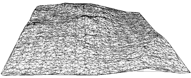
Figure 6: precision = $6$ bits, compression factor = $5.44$

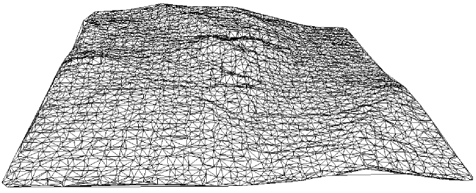
Figure 7: precision = $7$ bits, compression factor = $3.90$

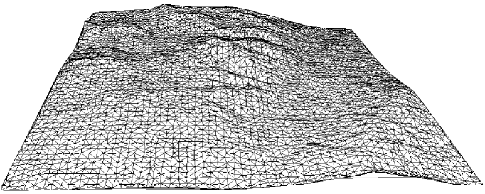
Figure 8: precision = $8$ bits, compression factor = $3.00$

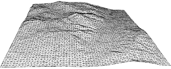
Figure 9: precision = $9$ bits, compression factor = $2.44$

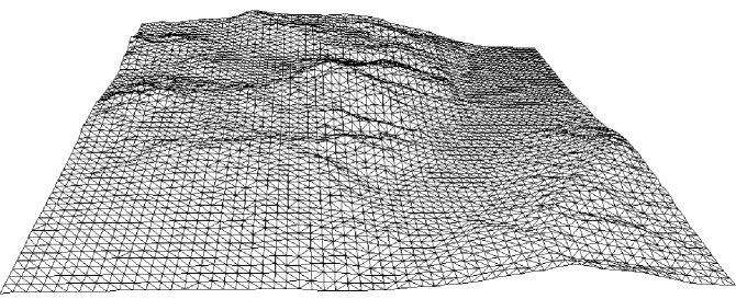
Figure 10: precision = $10$ bits (lossless compression), c. f. = $2.05$

References

- [1] N. Amenta and M. Bern. Surface reconstruction by Voronoi filtering. In Proc. 14th Annu. ACM Sympos. Comput. Geom., pages 39–48, 1998.
- [2] Fausto Bernardini and Chandrajit L. Bajaj. Sampling and reconstructing manifolds using alpha–shapes. In Proc. 9th Canad. Conf. Comput. Geom., pages 193–198, 1997.
- [3] Jean-Daniel Boissonnat and Bernhard Geiger. Three dimensional reconstruction of complex shapes based on the Delaunay triangulation. In R. S. Acharya and D. B. Goldgof, editors, Biomedical Image Processing and Biomedical Visualization, volume 1905, pages 964–975. SPIE, 1993.
- [4] M. Chow. Optimized geometry compression for real-time rendering. In Proc. IEEE Visualization, pages 347–354, 1997.
- [5] M. Deering. Geometry compression. In Proc. SIGGRAPH, pages 13–20, 1995.
- [6] R. Neal I. H. Witten and J. G. Cleary. Arithmetic coding for data compression. Communications of the ACM, 30(6):520–540, 1987.
- [7] J. Rissanen and G. G. Langdon. Arithmetic coding. IBM J. Res. Develop., 23(2):149–162, 1979.
- [8] J. Snoeyink and M. van Kreveld. Linear-time reconstruction of Delaunay triangulations with applications. In Proc. Annu. European Sympos. Algorithms, number 1284 in Lecture Notes Comput. Sci., pages 459–471. Springer-Verlag, 1997.
- [9] C. Sohler. Fast reconstruction of delaunay triangulations. In Proc. 11th Canad. Conf. Comput. Geometry, 1999.
- [10] G. Taubin and J. Rossignac. Geometric compression through topological surgery. Research Report RC-20340, IBM Research Division, 1996.
- [11] C. Touma and C. Gotsman. Triangle mesh compression. In Proc. Graphics Interface, pages 26–34, 1998.