Distributed Algorithms in Multihop Broadcast Networks

The paper addresses the problem of solving classic distributed algorithmic problems under the practical model of Broadcast Communication Networks. Our main result is a new Leader Election algorithm, with $O(n)$ time complexity and $O(n\cdot\lg(n))$ message transmission complexity. Our distributed solution uses a special form of the propagation of information with feedback (PIF) building block tuned to the broadcast media, and a special counting and joining approach for the election procedure phase. The latter is required for achieving the linear time.
It is demonstrated that the broadcast model requires solutions which are different from the classic point to point model.
Keywords: Broadcast networks, distributed, leader election.

1 Introduction

Broadcast networks are often used in modern communication systems. A common broadcast network is a single hop shared media system where a transmitted message is heard by all nodes. Such networks include local area networks like Ethernet and token-ring, as well as satellite and radio networks. In this paper we consider a more complex environment, in which a transmitted message is heard only by a group of neighboring nodes. Such environments include: Multihop packet radio networks, discussed for example in [CS89], [CW91]; Multichannel networks, in which nodes may communicate via several non-interfering communication channels at different bands [MR83]; and a wireless multistation backbone system for mobile communication [BDS83].
Since such networks are very important in the emerging area of backbone and wireless networks, it is important to design efficient algorithms for such environments. We address here the problem of finding efficient algorithms for classic network problems such as propagation of information and leader election in the new models.

In the classic model of network communication, the problem of leader election is reducible to the problem of finding a spanning tree. The classic model is a graph of $n$ nodes and $m$ edges, with the nodes representing computers that communicate via the edges which represent point-to-point bidirectional links. Gallager, Humblet and Spira introduced in their pioneering work [GHS83] a distributed minimum weight spanning tree (MST) algorithm, with $O(n\cdot\lg(n))$ time and $O(n\cdot\lg(n)+2\cdot m)$ message complexity. This algorithm is based on election phases in which the number of leadership candidates (each represents a fragment) is at least halved. Gallager et al. ensured a lower bound on a fragments level. In a later work, Chin and Ting [CT85] improved Gallager’s algorithm to $O(n\cdot lg^{*}(n))$ time, estimating the fragment’s size and updating its level accordingly, thus making a fragment’s level dependent upon its estimated size. In [Awe87], Awerbuch proposed an optimal $O(n)$ time and $O(n\cdot lg(n)+2\cdot m)$ message complexity algorithm, constructed in three phases. In the first phase, the number of nodes in the graph is established. In the second phase, a MST is built according to Gallager’s algorithm, until the fragments reach the size of $n/\lg(n)$. Finally, a second MST phase is performed, in which waiting fragments can upgrade their level, thus addressing a problem of long chains that existed in [GHS83], [CT85]. A later article by Faloutsos and Molle ([FM95]) addressed potential problems in Awerbuch’s algorithm. In a recent work Garay, Kutten and Peleg ([GKP98]) suggested an algorithm for leader election in $O(D)$ time, where $D$ is the diameter of the graph. In order to achieve the $O(D)$ time, they use two phases. The first is a controlled version of the GHS algorithm. The second phase uses a centralized algorithm, which concentrates on eliminating candidate edges in a pipelined approach. The message complexity of the algorithm is $O(m+n\cdot\sqrt{n}$).

It is clear that all of the above election algorithms are based on the fact that sending different messages to distinct neighbors is as costly a sending them the same message, which is not the case in our model. Our model enables us to take advantage of the broadcast topology, thus reducing the number of sent messages and increasing parallelism in the execution. Note, that while we can use distinct transmissions to neighbors it increases our message count due to unnecessary reception at all neighbors.
Algorithms that are based on the GHS algorithm, chose a leader via constructing a MST in the graph. First these algorithms distinguish between internal and external fragment edges, and between MST-chosen and rejected edges. An agreement on a minimal edge between adjacent fragments is done jointly by the two fragments, while other adjacent fragments may wait until they join and increase in level. In this paper it is seen that the broadcast environment requires a different approach, that will increase parallelism in the graph.

Our main goal is to develop efficient distributed algorithms for the new model. We approach this goal in steps. First, we present an algorithm for the basic task of Propagation of Information with Feedback (PIF) [Seg83] with $O(n)$ time and message transmission complexity. In the classic point-to-point model the PIF is an expensive building block due to its message complexity. The native broadcast enables us to devise a message efficient fragment-PIF algorithm, which provides a fast communication between clusters. Next, using the fragment-PIF as a building block, we present a new distributed algorithm for Leader Election, with $O(n)$ time and $O(n\cdot\lg(n))$ message transmission complexity. In order to prove correctness and establish the time and message complexity, we define and use an equivalent high level algorithm for fragments, presented as a state machine.
The paper is constructed as follows: Section 2 defines the the model. Section 3 presents a PIF algorithm suited for the model. Section 4 introduces a distributed Leader Election algorithm for this model and shows and proves properties of the algorithm. Section 5 presents some simulation results of the distributed leader election algorithm. We conclude with a summary of open issues.

2 The Model

A broadcast network can be viewed as a connected graph $G(V,E)$, where $V$ is the set of nodes. Nodes communicate by transmitting messages. If two nodes are able to hear each other’s transmissions, we define this capability by connecting them with an edge. A transmitted message is heard only by a group of neighboring nodes. In this paper we use the terms message and message transmission interchangeably. $E$ is the set of edges. All edges are bidirectional. In the case of radio networks, we assume equal transmission capacity on both sides.
Our model assumes that every node knows the number of its neighbors. The originator of a received message is known either by the form of communication, or by indication in the message’s header.
In the model, a transmitted message arrives in arbitrary final time to all the sender’s neighbors. Consecutive transmissions of a node arrive to all its neighbors in the same order they were originated, and without errors. We further assume that there are no link or node failures, and additions.
It should be noted, that we assume that the media access and data link problems, which are part of OSI layer 2 are already solved. The algorithms presented here are at higher layers, and therefore assume the presence of a reliable data link protocol which delivers messages reliably and in order. Bar-Yehuda, Goldreich and Itai ([BYGI92]) have addressed a lower level model of a multihop radio environment even with no collision detection mechanism. In their model, concurrent receptions at a node are lost. We assume models which are derived from conflict free allocation networks such as TDMA, FDMA or CDMA cellular networks, which maintain a concurrent broadcast environment with no losses.

3 Basic Propagation of Information Algorithms in our Model

The problem introduced here is of an arbitrary node that has a message it wants to transmit to all the nodes in the graph. The solution for this problem for the classic model of communication networks was introduced by [Seg83], and is called Propagation of Information (PI). The initiating node is ensured that after it has sent the message to its neighbors, all the nodes in the network will receive the message in finite time. An important addition to the PI algorithm is to provide the initiator node with knowledge of the propagation termination, i.e., when it is ensured that all the nodes in the network have received the message. This is done with a feedback process, also described in [Seg83] and added to the PI protocol. We describe a Propagation of Information with Feedback (PIF) algorithm for broadcast networks. Because of the unique character of broadcast networks, it is very easy to develop a PI algorithm for this environment. When a node gets a message for the first time it simply sends it once to all neighbors, and then ignores any additional messages. In the feedback process messages are sent backwards over a virtual spanned tree in the broadcast network, to the initiator node.

3.1 Algorithm Description

We describe here the Propagation of Information with Feedback. A message in this algorithm is of the form: MSG(target, l, parent), where target specifies the target node or nodes. A null value in the target header field indicates a broadcast to all neighboring nodes, and is used when broadcasting the message. The parent field specifies the identity of the parent of the node that sends the message. It is important to note that a node receives a message only when addressed in the target header field by its identification number or when this field is null. The $l$ field determines the sender’s identity. The initiator, called the source node, broadcasts a message, thus starting the propagation. Each node, upon receiving the message for the first time, stores the identity of the sender from which it got the message, which originated at the source, and broadcasts the message. The feedback process starts at the leaf nodes, which are childless nodes on the virtual tree spanned by the PIF algorithm. A leaf node that is participating in the propagation from the source, and has received the message from all of its neighboring nodes, sends back an acknowledgment message, called a feedback message, which is directed to its parent node. A node that got feedback messages from all of its child nodes, and has received the broadcasted message from all of its neighboring nodes sends the feedback message to its parent. The algorithm terminates when the source node gets broadcast messages from all of its neighboring nodes, and feedback messages from all of its child neighboring nodes.
Formal description of the algorithm can be found in Appendix B.

3.2 Properties of the Algorithm

We define here the properties of the PIF algorithm in a broadcast network. Because of the similarity to the classic model, the time and message complexity is $O(n)$.

Theorem 3.1

Suppose a source node $i$ initiates a propagation of a message at time $t=\tau$. Then, we can say the following:

• All nodes $j$ connected to $i$ will receive the message in finite time.

• Each node in the network sends one message during the propagation, and one message during the acknowledgment, to the total of two messages.

• The source node $i$ will get the last feedback message at no later than $\tau+2\cdot n$ time units.

• The set of nodes formed by the set $\{parent_{s}\cup i\}$ nodes spans a virtual tree of fastest routes, from the source node, on the graph.

The proof is similar to [Seg83].

4 Leader Election

The leader election algorithm goal is to mark a single node in the graph as a leader and to provide its identity to all other nodes.

4.1 The Algorithm

During the operation of the algorithm the nodes are partitioned into fragments. Each fragment is a collection of nodes, consisting of a candidate node and its domain of supportive nodes. When the algorithm starts all the candidates in the graph are active. During the course of the algorithm, a candidate may become inactive, in which case its fragment joins an active candidate’s fragment and no longer exists as an independent fragment. The algorithm terminates when there is only one candidate in the graph, and its domain includes all of the nodes. First, we present a higher level algorithm that operates at the fragment level. We term this algorithm the general algorithm. We then present the actual distributed algorithm by elaborating upon the specific action of individual nodes. In order to establish our complexity and time bounds we prove correctness of the general algorithm, and then prove that the general and distributed leader election algorithms are equivalent. We do so by proving that every execution of the general algorithm, specifically the distributed one, behaves in the same manner. We conclude by proving the properties and correctness of the algorithm.

4.1.1 The General Algorithm for a Fragment in the graph

We define for each fragment an identity, denoted by $id(F)$, and a state. The identity of a fragment consists of the size of the fragment, denoted by id.size and the candidate’s identification number, denoted by id(F).identity. The state of the fragment is either work, wait or leader. We associate two variables with each edge in the graph, its current state and its current direction. An edge can be either in the state internal, in which case it connects two nodes that belong to the same fragment, or in the state external, when it connects two nodes that belong to different fragments. External edges will be directed in the following manner: Let $e$ be an external edge that connects two different fragments $F1$ and $F2$. The algorithm follows these definitions for directing an edge in the graph:

Definition 4.1

The lexicographical relation $id(F1)>id(F2)$ holds if: $id(F1).size>id(F2).size$
or if $[id(F1).size=id(F2).size$ and $id(F1).identity>id(F2).identity]$.

Definition 4.2

Let $e$ be the directed edge $(F1,F2)$ if $id(F1)>id(F2)$ as defined by definition 4.1

If the relation above holds, $e$ is considered an outgoing edge for fragment $F1$ and an incoming edge for fragment $F2$, and fragments $F1$ and $F2$ are considered neighboring fragments. We assume that when an edge changes its direction, it does so in zero time.

Figure 1: A Fragment State Machine

When the algorithm starts, each node is an active candidate, with a fragment size of 1. We describe the algorithm for every fragment in the graph by a state machine as shown in Figure 1. A fragment may be in one of the following states: wait, work or leader. A Fragment is in the virtual state cease-to-exist when it joins another candidate’s fragment. The initial state for all fragments is wait, and the algorithm terminates when there is a fragment in the leader state. During the course of the algorithm, a fragment may move between states only when it satisfies the transition condition, as specified by the state machine.
The delays within the states are defined as follows: waitdelay - A delay a fragment suffers while in the wait state, while waiting for other fragments to inform of their identity. workdelay- This is a delay each fragment suffers while in the work state. Both delays are arbitrary limited, positive delays. The transition conditions are: Cwait which is defined by rule 2(b)i below, Cleader which is defined by rule 3 below, Ccease which is defined by rule 2(b)ii below and Cwork which is defined by rule 1 below. None of the transition conditions can cause any delay in time. The transition conditions are the following: Cwait- The transition condition from the work state to the wait state. The condition is defined by rule 2(b)i below. Cleader- The transition condition from work state to leader state. The condition is defined by rule 3 below. Ccease- The transition condition from the work state to the cease-to-exist virtual state. The condition is defined by rule 2(b)ii below. Cwork - The transition condition from wait state to work state. The condition is defined by rule 1 below.

The State Machine Formal Description:

1. A fragment $F$ enters the wait state when it has at least one outgoing edge (Cwait condition definition).

2. A Fragment $F$ transfers to the work state from the wait state (Cwork condition definition) when all its external edges are incoming edges. In the work state, the fragment will incur a delay named workdelay, while it performs the following:

   1. Count the new number of nodes in its current domain. The new size is kept in the variable new_size. We define the delay caused by the counting process by countdelay.

   2. Compare its new_size to the size of its maximal neighbor fragment, $F^{\prime}$.

      1. If $new\_size(F)>X\cdot id(F^{\prime}).size$ then fragment $F$ remains active. ($X>1$, a parameter. The optimal value of $X$ is calculated in Section 4.3).
         Let $id(F).size\leftarrow new\_size$. $F$ changes all of its external edges to the outgoing state. (clearly, definition 4.2 holds here and at this step, all of its neighbors become aware of its new size.) We define the delay caused by notifying the neighboring fragments of its new size by innerdelay. At this stage, condition Cwait is satisfied, and $F$ transfers to the wait state.

      2. Else, condition Ccease is satisfied, and $F$ ceases being an active fragment and becomes a part of its maximal neighbor fragment $F^{\prime}$. External edges between $F$ and $F^{\prime}$ will become internal edges of $F^{\prime}$. $F^{\prime}$ does not change its size or id, but may have new external edges, which connect it through the former fragment $F$ to other fragments. The new external edges’ state and direction are calculated according to the current size of $F^{\prime}$. It is clear that all of them will be outgoing edges at this stage. We define the delay caused by notifying all of the fragment’s nodes of the new candidate id innerdelay.

3. A Fragment that has no external edges is in the leader state. (Cleader condition definition).

4.1.2 The Distributed Algorithm for Nodes in the Graph

We describe here the distributed algorithm for finding a leader in the graph. In Theorem 4.2 we prove that this algorithm is equivalent to the general algorithm presented above.
When the algorithm starts, each node in the graph is an active candidate. During the course of the algorithm, the nodes are partitioned into fragments, supporting the fragment’s candidate. Each node always belong to a certain fragment. Candidates may become inactive and instruct their fragment to join other fragments in support of another candidate. A fragment in the work state may remain active if it is $X$ times bigger than its maximal neighbor. The information within the fragment is transfered in PIF cycles, originating at the candidate node. The feedback process within each fragment starts at nodes called edge nodes. An edge node in a fragment is either a leaf node in the spanned PIF tree within the fragment, or has neighboring nodes that belong to other fragments. The algorithm terminates when there is one fragment that spans all the nodes in the graph.

Definition 4.3

Let us define a PIF in a fragment, called a fragment-PIF, in the following manner:

• The source node is usually the candidate node. All nodes in the fragment recognize the candidate’s identity. When a fragment decides to join another fragment, the source node is one of the edge nodes, which has neighbor nodes in the joined fragment (the winning fragment).

• All the nodes that belong to the same fragment broadcast the fragment-PIF message which originated at their candidate’s node, and no other fragment-PIF message.

• An edge node, which has no child nodes in its fragment, initiates a feedback message in the fragment-PIF when it has received broadcast messages from all of its neighbors, either in its own fragment or from neighboring fragments.

Algorithm Description
The algorithm begins with an initialization phase, in which every node, which is a fragment of size $1$, broadcasts its identity. During the course of the algorithm, a fragment that all of its edge nodes have heard PIF messages from all their neighbors enter state work. The fragment’s nodes report back to the candidate node the number of nodes in the fragment, and the identity of the maximal neighbor. During the report, the nodes also store a path to the edge node which is adjacent to the maximal neighbor. The candidate node, at this stage also the source node, compares the newly counted fragment size to the maximal known neighbor fragment size. If the newly counted size is not at least $X$ times bigger than the size of the maximal neighbor fragment, then the fragment becomes inactive and joins its maximal neighbor. It is done in the following manner: The candidate node sends a message, on the stored path, to the fragment’s edge node. This edge node becomes the fragment’s source node. It broadcasts the new fragment identity, which is the joined fragment identity. At this stage, neighboring nodes of the joined fragment disregard this message, thus the maximal neighbor fragment will not enter state work. The source node chooses one of its maximal fragment neighbor nodes as its parent node, and later on will report to that node. From this point, the joining fragment broadcasts the new identity to all other neighbors. In case the newly counted size was at least $X$ times that of the maximal neighboring fragment, the candidate updates the fragment’s identity accordingly, and broadcasts it. (Note, this is actually the beginning of a new fragment-PIF cycle.) The algorithm terminates when a candidate node learns that it has no neighbors.
Appendix C contains a more detailed description, as well as a mapping of the transition conditions and the delays in the general algorithm to the distributed algorithm.

4.2 Properties of the Algorithm

In this section we prove that a single candidate is elected in every execution of the algorithm. Throughout this section we refer to the high level algorithm, and then prove consistency between the versions. All proofs of lemmas and theorems in this section appear in Appendix A.

Theorem 4.1

If a nonempty set of candidates start the leader election algorithm, then the algorithm eventually terminates and exactly one candidate is known as the leader.

Theorem 4.2

If all the nodes in the graph are given different identities, then the sequence of events in the algorithm does not depend on state transition delays.

Corollary 1

If all the nodes in the graph are given different identities, then the identity of the leader node will be uniquely defined by the high level algorithm.

4.3 Time and Message Complexity

We prove in this section, that the time complexity of the algorithm is $O(n)$. It is further shown, that for $X=3$ the time bound is the minimal, and is $9\cdot n$. We also prove that the message complexity is $O(n\cdot lg(n))$.
In order to prove the time complexity, we omit an initialization phase, in which each node broadcasts one message. This stage is bounded by $n$ time units. (Note, that a specific node is delayed by no more than 2 time units - its message transmission, followed by its neighbors immediate response.)
Let us define a winning fragment at time $t$ during the execution of the algorithm to be a fragment which remained active after being in the work state. Thus, excluding the initialization phase, we can say the following:

Property 1

From the definitions and properties in Appendix C, it is clear that the delay workdelay for a fragment is bounded in time as follows: (a) For a fragment that remains active, the delay is the sum of countdelay and innerdelay. (b) For a fragment that becomes inactive, it is the sum: countdelay $+2\cdot$ innerdelay.

Theorem 4.3

Let $t^{j}_{i}$ be the time measured from the start, in which a winning fragment $F_{j}$ completed the work state at size $k_{i}$. Then, assuming that $workdelay_{i}^{j}\leq 3\cdot k_{i}$, and that $countdelay^{j}_{i}\leq k_{i}$, we get that:

$$t^{j}_{i}\leq\frac{X^{2}+3\cdot X}{X-1}\cdot k_{i}$$

Proof of Theorem 4.3

We prove by induction on all times in which fragments in the graph enter state work, denoted $\{t^{j}_{i}\}$.
$t_{1}$: The minimum over $t_{i}^{j}$ for all $j$. It is clear that the lemma holds.
Let us assume correctness for time $t_{i}^{j}$, and prove for time $t_{i}^{j}+workdelay_{i}^{j}$, for any $j$.
From lemma 4 we deduct that $k_{i}>X^{2}\cdot k_{i-1}$. Therefore, according to the induction assumption, $F_{j}$ entered state $work$ for the $i-1$ time in time: $t^{j}_{i-1}\leq\frac{X^{2}+3\cdot X}{X-1}\cdot k_{i-1}$. Let us now examine the time it took $F_{j}$ to grow from its size at time $t^{j}_{i-1}$ to size $k_{i}$,: $t^{j}_{i}-t^{j}_{i-1}$. Since $F_{j}$ is a winning fragment at time $t^{j}_{i}$, it is at least $X$ times the size of any of its neighboring fragments. In the worst case, the fragment has to wait for a total of size $(X-1)\cdot\frac{k_{i}}{X}$ that joins it. Note, that the induction assumption holds for all of $F_{j}$’s neighbors. So we stated that:

1. The time it took a winning fragment to get to size $k_{i-1}$ is $t^{j}_{i-1}$, and $k_{i-1}\leq 1/X^{2}\cdot k_{i}$

2. The fragment then entered the work state to discover that its actual size is $k^{`j}_{i-1}\leq 1/X\cdot k_{i}$

3. $F$ has to wait for joining fragments, in the overall size of: $(X-1)\cdot 1/X\cdot k_{i}$

4. The time it takes the fragment’s candidate of size $k_{i}$ to be aware of its neighboring fragments identities and its own size while in the work state is bounded by $countdelay_{i}^{j}\leq k_{i}$.

From items 1 to 4 we can conclude that:
$t^{j}_{i}\leq\frac{X^{2}+3\cdot X}{X-1}\cdot k_{i-1}+workdelay^{j}_{i-1}+\frac{X^{2}+3\cdot X}{X-1}\cdot(X-1)\cdot\frac{1}{X}\cdot k_{i}+countdelay_{i}^{j}\\ ~{}~{}~{}~{}\leq\frac{X^{2}+3\cdot X}{X-1}\cdot\frac{1}{X^{2}}\cdot k_{i}+3\cdot\frac{1}{X}\cdot k_{i}+\frac{X^{2}+3\cdot X}{X-1}\cdot(X-1)\cdot\frac{1}{X}\cdot k_{i}+k_{i}\\ ~{}~{}~{}~{}=\frac{X^{2}+3\cdot X}{X-1}\cdot k_{i}$ $\Box$

Corollary 2

From property 1 it is obtained that the delay workdelay for every fragment of size $k$ is indeed bounded by $3\cdot k$, and that the delay countdelay is bounded by $k$. Therefore, from Theorem 4.3 the time it takes the distributed algorithm to finish is also bounded by

$$t^{j}_{i}\leq\frac{X^{2}+3\cdot X}{X-1}\cdot n$$

where $n$ is the number of nodes in the graph, and therefore is $O(n)$.

Corollary 3

When $X=3$ the algorithm time bound is at its minimum: $t^{j}_{i}\leq 9\cdot n$.

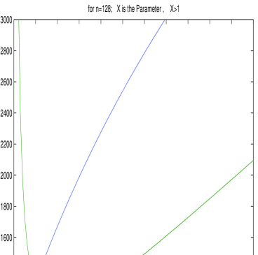
Figure 2: Time and Message Complexity as a factor of X

Theorem 4.4

The number of messages sent during the execution of the algorithm is bounded by:

$$(\frac{lg(n)-lg(1+X)}{lg(\frac{X+1}{X})}+1)\cdot n\hskip 5.69054pt;\hskip 14.22636ptX>1$$

.

The proof of Theorem 4.4 is in Appendix A.

5 Simulation results

The Distributed Leader Election was simulated using SES/Workbench, which is a graphical event driven simulation tool. The algorithm was simulated for a multihop broadcast environment. The algorithm was tested for a wide range of different topologies, among them binary trees, rings and strings, as well as more connected topologies. The simulation enables the user to choose the number of nodes, a basic topology, the connectivity and the growth factor $X$. The simulation output consists of the identity of the chosen leader node, the total time it took to get to the decision (excluding initialization phase) and the number of transmissions sent during the course of the algorithm.

Our simulation program first generates a random topology for the operation of the algorithm. The method for building the topology is based on an initial simple connected graph (tree, string, ring, etc.) and a random addition of edges to that initial graph. We present here results of two initial graphs: strings and binary trees. The numbered nodes are randomly arranged into the given initial graph. Then, adhering to the connectivity parameter and correctness, edges are randomly added to the graph. The connectivity parameter, $C$, is defined as the ratio between the number of additional edges in the graph out of all possible edges. For each topology and connectivity 100 different graphs were generated and executed.

We present here the maximal time and transmission results measured for each topology and connectivity, for a fixed number of nodes and the same growth factor. Figure 3 and Figure 4 present the maximal measured time for string and binary tree based topologies, respectively. The slowest measured topology is a pure string, since it does not exploit the broadcast ability. Minimal time for both topologies is measured for connectivity of 20%-30%. In both cases, the measured time is less than the number of nodes, due to maximal parallelism in the algorithm. As connectivity grows, the algorithm loses parallelism.

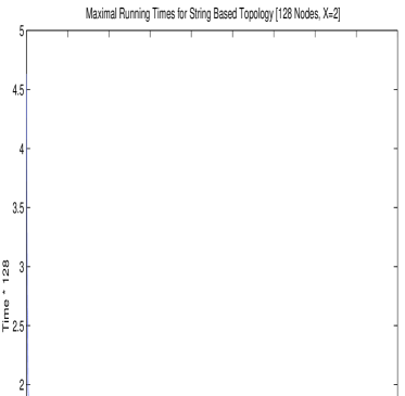
Figure 3: Maximal Times for String Based Topologies

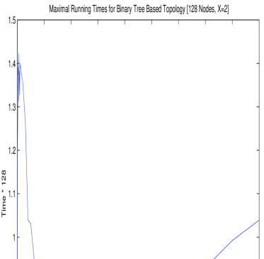
Figure 4: Maximal Times for Binary Tree Based Topologies

Our results show that for connectivity of 20 % and up, the maximal identity node was chosen the leader of the graph in most cases, and from connectivity of 30% and up it was always selected. This scenario best suits the case of a fully connected graph, in which all nodes are aware of all possible identities as soon as the initialization phase is over. Thereafter, each node, starting with the minimal identity node, joins the maximal identity node by order of increasing identities. In the case of a fully connected graph, there is a strict increasing order of joining among the nodes. When connectivity is 20% to 30% , the maximal identity node is well known in the graph, but parallelism is high. This leads to a situation in which nodes join the maximal identity node without waiting for each other, and the leader is chosen very quickly.

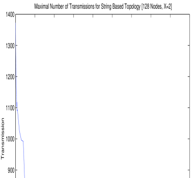
Figure 5: Maximal Transmissions for String Based Topologies

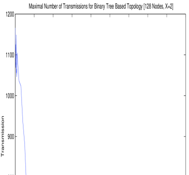
Figure 6: Maximal Transmissions for Binary Tree Based Topologies

Figure 5 and Figure 6 present maximal measured transmissions for a string based topology and a binary tree based topology. It can be observed, that generally higher connectivity means less transmissions. This follows the order scheme discussed earlier for densed graphs, in which the maximal identity node is known throughout the graph and rarely has any competition. This leads to a situation in which nodes join the winning candidate very early in the algorithm, and do not participate in unnecessary work states.

6 Summary

We presented new distributed algorithms for emerging modern broadcast communication systems. Under the new model we introduced algorithms for PIF and Leader Election. The algorithms are optimal in time and message complexity.
By using the fragment-PIF approach our leader election algorithm enables a fragment to affect all of its neighbors concurrently, thus increasing parallelism in the graph. This new approach may be used for all fragment-based decision algorithms in a broadcast environment.

There are several more problems to investigate under this model, such as other basic algorithms (e.g. DFS), failure detection and recovery. Other environments, such as a multicast environment, may require different approaches. Extensions of the model might also be viewed. Broadcast LANs are often connected via bridges. This leads to a more general model that includes both point to point edges and a broadcast group of edges connected to each node. For such a general model, the design of specific algorithms is required as well.

Appendix A

Proof of Theorem 4.1

In order to proof the Theorem, we will state some Properties and Lemmas.

Property 2

When an active fragment changes its state from work to wait, all of its external edges are outgoing edges.

Lemma 1

During every execution of the algorithm, at least one active candidate exists.

Proof of Lemma 1

By definition, an active candidate exists in the graph either in the work, wait or leader state. A candidate becomes inactive according to the algorithm if it discovers, while in the work state, an active neighbor fragment of bigger size, as can be seen in 2(b)ii. By this definition it is clear that a candidate may cease to exist only if it encountered another active candidate of at least half its size. Therefore, during the execution of the algorithm, there will always be at least one active candidate. $\Box$

Property 3

When an active fragment changes its state from work to wait, all of its external edges are outgoing edges.

Lemma 2

During the execution of the algorithm, there is always a fragment in the work or leader states.

Proof of Lemma 2

A fragment will be in the work state if it has the minimal $id$ among all its neighbors. Definition 4.1 determines that the fragment’s $id$ consists of its size and identity number. If there exists a fragment of minimal size, then it is the fragment with the minimal $id$. Otherwise, there are at least two fragments in the graph that have the same minimal size. As defined, the fragment with the lower identity number has the lower $id$. It is clear then, that at any stage of the algorithm there exists a fragment with a minimal $id$, and therefore there will always be a fragment in the work or leader state. $\Box$

Lemma 3

If a fragment $F$ was in the work state and remained active in wait state, it will enter the work state again only after each and every one of its neighboring fragments has been in the work state as well.

Proof of Lemma 3

According to Property 3, when $F$ entered the wait state, all of its edges are in the outgoing state. In order to enter the work state again, all of $F$’s external edges have to be incoming edges. While in the wait state, $F$ does nothing. Its neighbor activity is the only cause for a change in the edges’ state or direction. An outgoing edge may change its state to internal, if the neighbor fragment enters the work state and becomes a supporter of $F$ or changes its direction to incoming, according to Definition 4.2, as a result of a neighbor fragment changing its size. Hence, all $F$’s neighboring fragments must be in the work state before $F$ may enter it again. $\Box$

Corollary 4

A fragment $F$ in the wait state which has a neighbor fragment $F^{\prime}$ in the work state may enter the work state only after $F^{\prime}$ has changed its state to the wait state.

Lemma 4

Let us consider a fragment, $F$, that entered the work state for two consecutive times, $i$ and $i$+1 and remained active. Let $t_{i}$ be the time it entered the work state for the $i$-$th$ time, and let $t_{i+1}$ be the $i$+1 time. Let us define by $k_{i}$ its known size at time $t_{i}$, and by size $k_{i+1}$ its size at time $t_{i+1}$+ countdelay. Then, $k_{i+1}\geq X^{2}\cdot k_{i}$.

Proof of Lemma 4

If $F$ enters the work state for the $i$-$th$ time at time $t_{i}$, then according to Lemma 3 all of its neighbor fragments will be in the work state before time $t_{i+1}$. We know that at time $t_{i}$ $F$ is of known size $k_{i}$. According to rules 2(b)ii and 2(b)i, if it stayed active, it has enlarged its size by a factor of $X$ at least. (Note, $X>1$). Since $F$ reentered the work state, any of its new neighboring fragments is at least as big as F, i.e. at size of at least $X\cdot k_{i}$. We know that $F$ remains active after completing both work states. Therefore, following the same rules [ 2(b)ii and 2(b)i ], at time $t_{i+1}$+countdelay, its size, $k_{i+1}$, must be at least $X$ times the size of its maximal neighbor. It follows directly that $k_{i+1}\geq X^{2}\cdot k_{i}$. $\Box$

Corollary 5

The maximal number of periods that an active candidate will be in the work state is $\lg_{X}{n}$.

Now we can proceed with the Theorem:
From Lemma 1 and Lemma 2 it is clear that the algorithm does not deadlock, and that the set of active candidates is non-empty throughout the course of the algorithm. Property 5 limits the number of times a candidate may enter the work state. Since at any time there is a candidate in the work state, there always exists a candidate that enlarges its domain. It follows that there exists a stage in the algorithm where there will be only one candidate, and its domain will include all the nodes in the graph. $\Box$

Proof of Theorem 4.2

Let $U$ be the set of fragments in the work state at any arbitrary time during the execution of the general algorithm. If we view the times before a fragment in the graph enters the leader state, then by lemma 2 and corollary 4 we can conclude that:

1. $U$ is non-empty until a leader is elected

2. Fragments in $U$ cannot be neighbors

3. All the neighboring fragments of a fragment $F\subseteq U$ cannot change their size until $F$ is no longer in $U$ (i.e., $F$ completes the work state and changes its state to wait).

At every moment during the execution of the algorithm, the graph is acyclic and the edges’ directions determine uniquely which fragments are in the work state. Let us examine the state of the graph at an arbitrary time, before any fragment enters the leader state. The conclusions above imply that there is a predetermined order in which fragments enter the work state. The time it takes a fragment to enter the work state from the wait state is determined by the Cwork condition. Excluding initialization, a fragment can reenter the work state after each of its neighboring fragments completed a period in the work state. The duration within the work state for a fragment, depends only on the local delay workdelay as defined by 1. Therefore, fragments that enter the work state complete it in finite time. Therefore, it is clear, that the order by which the fragment’s neighbors enter the work state does not affect the order by which it enters the work state. This proves that the sequence of events between every pair of neighboring fragments in the graph is predetermined, given the nodes have different identities. Therefore, the sequence of events between all the fragments in the graph is predetermined and cannot be changed throughout the execution of the algorithm. $\Box$

Proof of Theorem 4.4

In order to prove the Theorem, we use the following Lemmas and properties.

Property 4

During the execution of the algorithm, nodes within a fragment send messages only while in the work state.

Lemma 5

While in the work state, the number of messages sent in a fragment is at most $3\cdot k$, where $k$ is the number of nodes within the fragment.

Proof of Lemma 5

While in the work state, each node can send either one of three messages: FEEDBACK, ACTION and INFO (in this order). Every message is sent only once, from the PIF properties. Therefore, the number of messages sent in a fragment of size $k$ is bounded by $3\cdot k$. $\Box$

Lemma 6

Let $l$ be the number of times a cluster of nodes, initially a fragment, entered state work. Then:

$$l=\frac{lg(n)-lg(1+X)}{lg(\frac{X+1}{X})}+1$$

Proof of Lemma 6

A fragment of an arbitrary size $k$, may join a fragment of size $\frac{1}{X}\cdot k+1$. Therefore, $\forall l$, the minimal growth rate is of the form: $k_{l}=k_{l-1}+\frac{1}{X}\cdot k_{l-1}+1=\frac{X+1}{X}\cdot k_{l-1}+1$ , where $k_{0}=0$.
Let us define the following:

$$k_{l}=a\cdot k_{l-1}+1;\hskip 14.22636pta=\frac{X+1}{X};\hskip 14.22636pt\sum_{l=1}^{\infty}k_{l}\cdot Z^{l}=k(Z)$$

By using the $Z$ transform as defined above, it follows that:

$$k_{l}=a\cdot\sum_{l=1}^{\infty}k_{l-1}\cdot Z^{l}=a\cdot Z\cdot\sum_{l=1}^{\infty}k_{l-1}\cdot Z^{l-1}=a\cdot Z\cdot k(Z)$$

Since $k_{0}=0$ and $\forall Z<1,\sum_{l=0}^{\infty}Z^{l}=\frac{1}{1-Z}$, we obtain that:

$$k(Z)=a\cdot Z\cdot k(Z)+\frac{1}{1-Z}\hskip 8.53581pt\Rightarrow\hskip 8.53581ptk(Z)=\frac{1}{(1-Z)\cdot(1-a\cdot Z)}$$

By separation of variables we get:

$$k(Z)=\frac{X+1}{1-a\cdot Z}-\frac{X}{1-Z}$$

Therefore:

$$\sum_{l=1}^{\infty}k_{l}\cdot Z^{l}=(X+1)\cdot\sum_{l=1}^{\infty}(a\cdot l)^{l}-X\cdot\sum_{l=1}^{\infty}Z^{l}=\sum_{l=1}^{\infty}[(X+1)\cdot a^{l}-X]\cdot Z^{l}$$

Since by definition $a>1$, we get: $k_{l}=(X+1)\cdot a^{l}-X\geq a^{l}+X\cdot a^{l}-X\geq a^{l-1}+X\cdot a^{l-1}=(1+X)\cdot a^{l-1}.$ We require that: $(1+X)\cdot a^{l-1}=n$, where $n$ is the number of nodes in the graph. By taking the logarithm of both sides, we obtain:

$$l=\frac{lg(n)-lg(1+X)}{lg(\frac{X+1}{X})}+1$$

$\Box$
Now we may proceed to prove the message complexity:
From Property 4 it is clear that every fragment sends messages only while it is in the work state. Lemma 5 shows that in the work state, the maximal number of messages sent within a fragment of size $k$ is $3\cdot k$. From Lemma 6 and the above we obtain that the message complexity is:

$$(\frac{lg(n)-lg(1+X)}{lg(\frac{X+1}{X})}+1)\cdot n\hskip 5.69054pt;\hskip 14.22636ptX>1$$

. $\Box$

Appendix B

Propagation of Information with Feedback Formal Description

Protocol messages

$START$

– Upon receiving a $START$ message a node will initialize its internal protocol variables and initiates propagation of an information in the network. A $START$ message may be delivered to an undetermined number of nodes, each of which will initiates an independent propagation of information in the network.

$MSG$

– The message propagated in the network. The propagation comes to an end when The starting nodes gets it back from all of its descendants nodes.

Each protocol message includes the following data:

$target$

– Specifies the target node or nodes. zero will indicate all neighboring nodes.

$l$

– The sender’s identification.

$parent$

– The sender’s parent node. zero if none.

Each Node uses the following variables:

$i$

– The node’s identity

$l$

– The message sender’s identity

$parent$

– The node’s parent’s identity (zero for a start node)

The algorithm for a starting node $s$

• For a $START(s,s,0)$ message:

• set $m\leftarrow$ 1; set $parent\leftarrow$ 0; Send $MSG(0,s,parent)$

• For a $MSG(target,\ell,parent)$ message:
  $\ll$ Message is ignored if $parent$=$s$ AND $target\neq s$ $\gg$

• if $parent$ = $s$ AND $target\neq s$ IGNORE

• else:

• set $N(l)\leftarrow$ $1$

• if $\forall\ell~{}N(\ell)=1$ END

The Algorithm for a node i

• For a $MSG(target,\ell,parent)$ message received at node i:
  $\ll$ Message is ignored if $parent$=$s$ AND $target\neq s$ $\gg$

• if $parent$ = $s$ AND $target\neq s$ IGNORE

• else:

• set $N(l)\leftarrow$ $1$

• if $m$ = 0 : set $m\leftarrow$ 1; set $parent\leftarrow$ $\ell$; send $MSG(0,i,parent)$

• if $\forall\ell~{}N(\ell)=1$ send $MSG(parent,i,parent)$ on the link to $parent$.

Appendix C

Distributed Algorithm for Leader Election - Detailed Description

The messages sent

[All messages include additional fragment-PIF header fields.]

1. A broadcast INFO message from the source node of the fragment with the following data fields: A fragment’s current size and identity and a field that denotes the former fragment’s identity, for recognition within the fragment.

2. A FEEDBACK message, sent during the feedback phase. The message data field includes the accumulated number of nodes under this node in the fragment. It also includes a flag, indicating whether another neighboring fragment was encountered. If this flag is set, then the next two fields indicate the maximal neighbor fragment’s size and identity.

3. An ACTION message, sent only in case the fragment’s candidate observes that it has a neighboring fragment it should join. In this case it sends this message to one of its edge nodes, that has neighboring nodes in the joined fragment.

A detailed description

Initialization: The algorithm starts when an arbitrary number of nodes initialize their state and send an initialization INFO message, with their identity. Upon receiving such a message, a node sends its INFO message if it hasn’t done so yet, and notes the maximal and minimal identity it has encountered. When a node has received such INFO messages from all of its neighbors, it determines its state. If the node has the minimal identity amongst all of its neighbors, then it is in the work state, otherwise it is in the wait state. A node that enters the work state joins its maximal neighbor, initializes all of its inner variables accordingly, and broadcasts its INFO message, stating its maximal neighbor as its parent. A node in the wait state initializes all of its inner variables.

Propagation of INFO in a fragment: All the nodes that belong to the candidate’s fragment, upon first receiving a message that includes their fragment’s identity, do the following: note the fragment’s new identity as delivered in the message, record the identity of the node from which the message was first received in a parent variable, and broadcast the message.

Encountering another fragment: An edge node, which receives for the first time a broadcast message from a neighbor node that belongs to another fragment, sets an internal flag, and records the $id$ of the encountered fragment. It also records the identity of the node the message came from. If it receives additional broadcast messages from other fragments, it compares the $id$ delivered in the message to its registered one, according to definition 4.1, and records in its internal variables the maximal size fragment it has encountered, and the identity of the node which sent the message.

Initiating FEEDBACK: An edge node with no child nodes which has received a broadcast message from all of its neighbors, initiates a feedback message to its parent node. In the message it registers that it has encountered other fragments, and the maximal fragment $id$ it has encountered. The accumulated value of nodes under it is set to 1 and is sent. The node registers the number of neighboring nodes that belong to the maximal fragment and reinitializes the variables that belong to the fragment-PIF.

FEEDBACK process in a Fragment: A node that receives a FEEDBACK message from one of its child nodes, compares the $id$ of the maximal neighboring fragment its child node knows of to the one it knows of. If the node does not know yet of another fragment encountered, or if the $id$ delivered by the child node is bigger than the current known neighboring fragment’s $id$, according to definition 4.1, the node registers the $id$ of the maximal neighbor fragment in its internal variables, and registers the child node’s identity for a possible return path. It also adds the accumulated size of the sub-fragment under its child node to the current known count. A node that has received broadcast messages from all of its neighboring nodes and feedback messages from all of its child nodes, and is not the candidate node, sends a feedback message to its parent node, which includes the accumulated size of the sub-fragment under it, and the maximal known neighbor fragment $id$, if any. The node then reinitializes the fragment-PIF variables. A candidate node that has received broadcast messages from all of its neighbor nodes and FEEDBACK messages from all of its child nodes, compares the maximal known neighbor size, as delivered, to its new counted size and then follows according to conditions 1 or 2.

1. If its new size is at least twice the size of the maximal neighbor, then the candidate’s fragment remains active. The candidate then issues a new INFO message, with the fragment’s accumulated size, and sends its old fragment size for recognition purposes. It then updates its inner size variable to the sent one.

2. Else, the candidate decides to become inactive, and to join the maximal neighbor fragment. It does so by sending the ACTION message along the node path it has registered.

ACTION Message Process: A node which receives an ACTION message sends it along the path to the edge node. An edge node that receives an ACTION message from its parent node, does the following: It records the identity of the new fragment to join, and denotes the identity of the node from which it first heard of the other fragment as its parent node. It also initiates an INFO message, which contains the joined fragment’s identity as the new identity, and the old fragment’s identity, as sent in the ACTION message, as the old identity for recognition.

INFO Message Process: A node that receives an INFO message, can receive it from the following sources: (a) From its parent in its fragment. In this case, it records the new fragment’s identity or size, its parent node, and broadcasts the message. (b) From a neighbor in its fragment, in which case it registers the fact and ignores the message. (c) From an edge node in a joined fragment. If the node registers it as its parent node, it will reset the bit that indicates it has heard from it before, and await a FEEDBACK message from it. If not, it just ignores it.

Properties of the Distributed Algorithm
We introduce here a mapping of the states and transitions defined for the high level algorithm, as shown in Figure 1, to the distributed algorithm described above, and establish the delays within the states: The delay countdelay within a fragment starts when the last edge node to send a feedback message has done so. It ends when the candidate node of the fragment receives all of the INFO messages from its neighbor nodes, and all of the FEEDBACK messages from its child nodes.
The delay innerdelay within a fragment is defined as the time passed from the initiation of an INFO message by the source node until all the nodes in its fragment receive the message.
For a fragment of size $k$, both countdelay and innerdelay are bounded by $k$ time units, as can be seen from Theorem 3.1.
The delay innerdelay is also the maximal time it takes the candidate node to send an ACTION message to the new source node. Again, this can be seen from Theorem 3.1.
The delay workdelay for a fragment starts when the last edge node to send a FEEDBACK message has done so, and ends when the last node in the fragment receives the new INFO message.
The delay waitdelay for a fragment starts when the last node within a fragment receives the INFO message, and ends when the last edge node sends the FEEDBACK message.
Cwork is true if the last edge node within the fragment is able to send a FEEDBACK message.
Cleader is true if a candidate receives FEEDBACK messages from all of its fragment indicating that no other fragment was encountered.
Ccease is true if a candidate discovers it should become inactive and join another fragment.
Cwait is true if all the nodes within a fragment received a new INFO message originated at the source node.

References

- [Awe87] B. Awerbuch. Optimal distributed algorithms for minimum weight spanning tree, counting, leader election and related problems. Proc. 19th Symp. on Theory of Computing, pages 230 – 240, May 1987.
- [BDS83] A. Ben-David and M. Sidi. Collision resolution algorithms in multi-station packet radio network. IEEE Journal on Selected Areas in Communications, November 1983.
- [BYGI92] R. Bar-Yehuda, O. Goldreich, and A. Itai. On the time-complexity of broadcast in multi-hop radio netwroks: An exponential gap between determinism and randomization. Journal on Computer and System Sciences, 45:104–126, 1992.
- [CS89] I. Cidon and M. Sidi. Distributed assignment algorithm for multihop packet radio networks. IEEE Transaction on Computers, 38(10):1353 – 1361, October 1989.
- [CT85] F. Chin and H.F. Ting. An almost linear time and o(vlogv + e) message distributed algorithm for minimum weight spanning trees. Proceedings of Foundations Of Computer Science (FOCS), October 1985.
- [CW91] I. Chlamtac and O. Weinstein. The wave expansion approach to broadcasting in multihop radio networks. IEEE Transaction on Communications, COM-39(3):426 – 433, 1991.
- [FM95] M. Faloutsos and M. Molle. Optimal distributed algorithms for minimum spanning trees revisited. ACM Symp. on Principles of Distributed Computing, pages 231 – 237, May 1995.
- [GHS83] R. Gallager, P. Humblet, and P. Spira. A distributed algorithm for minimum weight spanning trees. ACM Transactions on Programming languages and Systems, 4(1):66 – 77, January 1983.
- [GKP98] J.A. Garay, S. Kutten, and D. Peleg. A sub-linear time distributed algorithm for minimum-weight spanning trees. SIAM Journal on Computing, pages 302–316, 1998.
- [MR83] M.A. Marsen and D. Roffinella. Multichannel local area network protocols. IEEE Journal on Selected Areas in Communications, SAC-1(5):885 – 897, November 1983.
- [Seg83] A. Segall. Distributed network protocols. IEEE Transaction on Information Theory, IT-29(1):23 – 35, January 1983.