Polygonal Chains Cannot Lock in 4D

Abstract

We prove that, in all dimensions $d\geq 4$, every simple open polygonal chain and every tree may be straightened, and every simple closed polygonal chain may be convexified. These reconfigurations can be achieved by algorithms that use polynomial time in the number of vertices, and result in a polynomial number of “moves.” These results contrast to those known for $d=2$, where trees can “lock,” and for $d=3$, where open and closed chains can lock.

1 Introduction

1.1 Summary

A polygonal chain $P=(v_{0},v_{1},\ldots,v_{n})$ is a sequence of consecutively joined segments $s_{i}=v_{i}v_{i+1}$ of fixed lengths $\ell_{i}=|s_{i}|$, embedded in space. A chain is closed if the line segments are joined in cyclic fashion, i.e., if $v_{n}=v_{0}$; otherwise, it is open. A polygonal tree is a collection of segments joined into a tree structure. A chain or tree is simple if only adjacent edges intersect, and only then at the endpoint they share. We study reconfigurations of simple polygonal chains and trees, continuous motions that preserve the lengths of all edges while maintaining simplicity. One basic goal is to determine if an open chain can be straightened—stretched out in a straight line, and whether a closed chain can be convexified—reconfigured to a planar convex polygon. For trees, straightening permits noncrossing violations of simplicity to allow the segments to align along the common straight line. If an open chain or tree cannot be straightened, or a closed chain convexified, it is called locked. This terminology is borrowed from [BDD⁺99] and [BDD⁺98].

Most of the work in this area was fueled by the longstanding open problem of determining whether every open (or closed) chain in 2D can be straightened (or convexified). This was recently settled [CDR00] in the affirmative: 2D chains cannot lock. In contrast it was earlier established that trees in 2D [BDD⁺98], and both open and closed chains in 3D [CJ98, BDD⁺99] can lock. In this paper we prove that, for all dimensions $d\geq 4$, neither chains (open or closed) nor trees can lock. We partition our results into four main theorems:

Theorem 1

Every simple open chain in 4D may be straightened, by an algorithm that runs in $O(n^{2})$ time and $O(n)$ space, and which accomplishes the straightening in $O(n)$ moves.

Here “move” is used in the sense defined in [BDD⁺99]. Essentially each move is a simple monotonic rotation of a few joints. We have implemented this algorithm for the case when the vertices are in general position, when it is straightforward.

Nearly the same algorithm proves the same result for trees, within the same bounds:

Theorem 2

Every simple tree in 4D may be straightened, by an algorithm that runs in $O(n^{2})$ time and $O(n)$ space, and which accomplishes the straightening in $O(n)$ moves.

Closed chains require more effort:

Theorem 3

Every simple closed chain in 4D may be convexified, by an algorithm that runs in $O(n^{6}\log n)$ time, and which accomplishes the straightening in $O(n^{6})$ moves.

All these results easily extend to higher dimensions:

Theorem 4

Theorems 1, 2, and 3 hold for all dimensions $d\geq 4$, i.e., neither polygonal chains nor trees can lock in dimensions greater than three.

We summarize our results in the context of earlier work in the table below.

Dimension	Chains	Trees
$2$	Cannot lock	Lockable
$3$	Lockable	Lockable
$d\geq 4$	Cannot lock	Cannot lock

1.2 Background

Before commencing with our technical arguments, we start with some background, with the intent of providing intuition to support our results.

No Knots in 4D.

In [CJ98] and [BDD⁺99], the same example of a locked open chain in 3D is provided. The version in the latter paper is shown in Fig. 1.

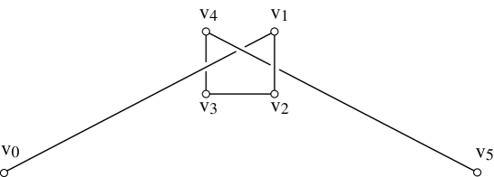
Figure 1: The “knitting needles” example, based on Fig. 1 in [BDD⁺99] (by permission).

One proof (used in [BDD⁺99]) that this chain $K$ is locked depends on closing the chain by connecting $v_{0}$ to $v_{5}$ to form $K^{\prime}$, and then arguing that $K$ can be straightened iff the corresponding trefoil knot $K^{\prime}$ can be unknotted, which of course it cannot. Thus there is a close connection in 3D between unknotted, locked chains and knots. However, the following theorem is well known:

Theorem 5

No 1D closed, tame, non-self-intersecting curve $C$ is knotted in $\mathbb{R}^{4}$.

See, e.g., [Ada94, pp.270-1] for an informal proof. Because proofs of this theorem employ topological deformations, it seems they are not easily modified to help settle our questions about chains in 4D. The rigidity of the links prevents any easy translation of the knot proof technique to polygonal chains. However, it does suggest that it would be difficult to construct a locked chain by extending the methods used in 3D.

No Cages in 4D.

A second consideration lends support to the intuition behind our main claim. This is the inability to confine one segment in a “cage” composed of other segments in 4D. Consider segment $s_{0}=v_{0}v_{1}$ in Fig. 1. It is surrounded by other segments in the sense that it cannot be rotated freely about one endpoint (say $v_{0}$) without colliding with the other segments. Let $S$ be the $2$-sphere in $\mathbb{R}^{3}$ of radius $\ell_{0}$ centered at $v_{0}$. Each point on $S$ is a possible location for $v_{1}$. Segment $s_{0}$ is confined in the sense that there are points of $S$ that cannot be reached from $s_{0}$’s initial position without collision with the other segments. This can be seen by centrally projecting the segments from $v_{0}$ onto $S$, producing an “obstruction diagram.” It should be clear that $v_{1}$ is confined to a cell of this diagram. Although this by no means implies that the chain in Fig. 1 is locked, it is at least part of the reason that the chain might be locked.

We now argue informally that such confinement is not possible in 4D. Again let $s_{0}=v_{0}v_{1}$ be fixed at $v_{0}$, and let $S$ be the $3$-sphere in $\mathbb{R}^{4}$ of radius $\ell_{0}$ centered on $v_{0}$ that represents the possible locations for $v_{1}$. Again we project the other segments onto $S$ producing an obstruction diagram. As in the lower dimensional case, this diagram is composed of 1D curves, being the projection of 1D segments. But in the $3$-sphere $S$, $v_{1}$ has three degrees of freedom, and cannot be confined by a (finite) set of 1D curves. Our next task is to make this intuitive argument more precise.

2 Straightening Open Chains in 4D

Let $P$ be a simple, open polygonal chain in 4D with $n\geq 2$ vertices. Each vertex $v_{i}$ is also called a joint of the chain. The segment $s_{i}=v_{i}v_{i+1}$ we sometimes call a link of the chain. We say a joint $v_{i}$ is straightened if $(v_{i-1},v_{i},v_{i+1})$ are collinear and form a simple chain; in this case, the angle at $v_{i}$ is $\pi$.

We prove Theorem 1 by straightening the first joint $v_{1}$, “freezing” it, and repeating the process until the entire chain has been straightened. This is a procedure which, of course, could not be carried out in 3D. But there is much more room for maneuvering in 4D. We have two different algorithms for accomplishing this task. The first (Algorithm 1a) is easier to understand, but only establishes a bound of $O(n^{4})$ on the number of moves, and requires $O(n^{4}\log n)$ time. The second (Algorithm 1b) is a bit more intricate but achieves $O(n)$ moves in $O(n^{2})$ time. Both follow the rough outline just sketched. We provide full details for Algorithm 1a, but only sketch Algorithm 1b.

Define the goal position $v_{g}$ for $v_{0}$ (and $s_{g}=v_{g}v_{1}$ the goal position for $s_{0}$) as the unique position that represents straightening of joint $v_{1}$. Call the goal position intersected if $s_{g}\cap s_{i}\neq\emptyset$ for some $i>2$; and otherwise call it free.

2.1 Algorithm 1a

A high-level view of the algorithm is as follows:

Algorithm 1a: Open Chains repeat until chain straightened do 1: if $s_{g}$ is free then Construct obstruction diagram Ob$(v_{0})$ on $3$-sphere. Apply motion planning to move $v_{0}$ to $v_{g}$. 2: else $s_{g}$ is intersected Construct obstruction diagram Ob$(v_{1})$ on $2$-sphere. Move $v_{1}$ so that the goal position is not intersected.

2.1.1 Step 1: $s_{g}$ is free

Our argument depends on some basic intersection facts, which we formulate in $\mathbb{R}^{d}$ in a series of lemmas before specializing to the $d=3$ and $d=4$ cases we need.

Geometric Intersections in $\mathbb{R}^{d}$.

Let the coordinates of $\mathbb{R}^{d}$ be $x_{1},x_{2},\ldots,x_{d}$. A $k$-flat is the translate of a subspace spanned by $k$ linearly independent vectors. Flats for $k=0,1,2$ are also called points, lines, and planes. A $k$-sphere is the set of points in a $(k+1)$-flat at a fixed radius from a point (its center) in that flat. A $0$-sphere is a set of two points, a circle is a $1$-sphere, and the surface of a ball in $\mathbb{R}^{3}$ is a $2$-sphere. When emphasizing the topology of a $k$-sphere, we will use the symbol $\mathbb{S}^{k}$.

Lemma 1

The intersection of a $2$-flat $H$ (i.e., a plane) with a $(d{-}1)$-sphere $S$ in $\mathbb{R}^{d}$ is a circle, a point, or empty.

Proof: Translate and rotate the sphere and plane so that the sphere is centered on the origin, and the plane is parallel to the $x_{1}x_{2}$-plane. The equations of the sphere $S$ and the plane $H$ are then:

$$S : x_{1}^{2}+x_{2}^{2}+\cdots+x_{d}^{2}=r^{2}$$ (1)

$$H : x_{3}=a_{3}\,,\,x_{4}=a_{4}\,,\,\cdots,\,x_{d}=a_{d}$$ (2)

where the $a_{i}$ are constants. Let $A^{2}=\sum_{i=3}^{d}a_{i}^{2}$. Then

$$S\cap H : x_{1}^{2}+x_{2}^{2}+A^{2}=r^{2}$$ (4)

$$x_{1}^{2}+x_{2}^{2}=r^{2}-A^{2}$$

If $r^{2}<A^{2}$, the intersection is empty. If $r^{2}=A^{2}$, the intersection is the point $(0,0,a_{3},\ldots,a_{d})$. If $r^{2}>A^{2}$, the intersection is a circle in $H$ with radius $\sqrt{r^{2}-A^{2}}$, and center $(0,0,a_{3},\ldots,a_{d})$. $\Box$

Lemma 2

The intersection of a (1D) line, ray, or segment with a $(d{-}1)$-sphere $S$ in $\mathbb{R}^{d}$ is at most two points, i.e., it either contains one or two points or is the empty set.

Proof: Let $s=ab$ be a segment, and let the sphere center be $c$. Let $H$ be the 2D plane determined by the three points $a,b,c$, i.e., $H$ is the affine span of $\{a,b,c\}$. Because $s\subset H$, we must have $s=s\cap H$. So

$$s\cap S = (s\cap H)\cap S$$ (5)

$$= s\cap(H\cap S)$$ (6)

By Lemma 1, $H\cap S$ is a circle, and the claim for segments follows because a segment intersects a circle in at most two points. Rays and lines yield the same result by selecting $a$ and $b$ sufficiently large. $\Box$

Let $a$, $b$, and $c$ be three distinct points in $\mathbb{R}^{d}$, such that $c$ does not lie on the segment $ab$. Call the set of points that lie on rays that start at $c$ and pass through a point of $ab$ a triangle cone ${\triangle}_{c}(a,b)$. If $(a,b,c)$ are collinear, the triangle cone degenerates to a ray.

Lemma 3

The intersection of a triangle cone ${\triangle}_{c}(a,b)$ with a $(d{-}1)$-sphere $S$ in $\mathbb{R}^{d}$ consists of at most two connected components—and, if $c$ is the center of $S$, of at most one component—each of which is a circular arc or a point.

Proof: Let ${\triangle}={\triangle}_{c}(a,b)$, and let $H$ be the 2D plane containing ${\triangle}$. Because ${\triangle}\subset H$, ${\triangle}={\triangle}\cap H$. So ${\triangle}\cap S={\triangle}\cap(H\cap S)$. By Lemma 1, $H\cap S$ is a circle $C$ in the plane containing ${\triangle}$. So the problem reduces to the intersection of a triangle cone with a circle. As illustrated in Fig. 2a, this intersection is at most one arc if the cone’s apex $c$ is at the center of the $C$ (${\triangle}_{1}$ in the figure), and at most two arcs otherwise (${\triangle}_{2}$ in the figure). Any of the arcs illustrated could degenerate to points if the cone is a ray. (When $c$ is not the center of $S$, the arc could be the whole circle $C$.) $\Box$

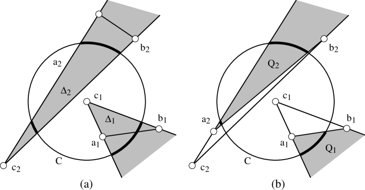
Figure 2: (a) Intersections of triangle cones ${\triangle}_{1}={\triangle}_{c_{1}}(a_{1},b_{1})$ and ${\triangle}_{2}={\triangle}_{c_{2}}(a_{2},b_{2})$ with a circle $C$ centered at $c_{1}$; (b) Intersections of quadrilateral cones $Q_{1}$ and $Q_{2}$ with $C$.

We will need a slight extension of this lemma. Define a quadrilateral cone $Q_{c}(a,b)$ to be the closure of ${\triangle}_{c}(a,b)\setminus t$, where $t$ is the triangle determined by $(a,b,c)$. Thus $Q_{c}(a,b)$ is all the points on the rays from $c$ at or beyond $ab$. The next lemma says that the conclusion of the previous lemma holds for quadrilateral cones as well.

Lemma 4

The intersection of a quadrilateral cone $Q_{c}(a,b)$ with a $(d{-}1)$-sphere $S$ in $\mathbb{R}^{d}$ consists of at most two connected components—and, if $c$ is the center of $S$, of at most one component—each of which is a circular arc or a point.

Proof: As Fig. 2b makes clear, $Q_{c}(a,b)$ is just ${\triangle}_{c}(a,b)$ intersected with a closed halfplane in $H$ containing $ab$. Intersecting the components from Lemma 3 with a halfplane cannot increase their number, and so the claim follows. $\Box$

Obstruction Diagram Ob$(v_{0})$.

Let ${\cal{C}}_{0}$ be the configuration space for vertex $v_{0}$ when $v_{1}$ is fixed: the set of all possible positions for $v_{0}$ that preserve the length of $v_{1}v_{0}$. ${\cal{C}}_{0}$ is a $3$-sphere $S$ in $\mathbb{R}^{4}$ centered at $v_{1}$ with radius $\ell_{0}$. Let ${\cal{F}}_{0}$ be the free space for vertex $v_{0}$ with all other vertices $v_{i}$ of the chain fixed: the subset of ${\cal{C}}_{0}$ for which the chain is simple, i.e., for which $s_{0}$ does not intersect $s_{i}$, $i>1$, and $s_{0}$ intersects $s_{1}$ only at $v_{1}$. We define the obstruction diagram ${{\rm Ob}(v_{0})}$ for $v_{0}$ as the set such that ${\cal{F}}_{0}={\cal{C}}_{0}\setminus{{\rm Ob}(v_{0})}$. Our goal is to describe, and ultimately construct, ${{\rm Ob}(v_{0})}$.

To ease notation, let ${}_{j}{\triangle}_{i}={\triangle}_{v_{j}}(v_{i},v_{i+1})$ be the triangle cone with apex $v_{j}$ determined by segment $i$, and define ${{}_{j}Q_{i}}\subseteq{{}_{j}{\triangle}_{i}}$ as the similar quadrilateral cone.

Lemma 5

The set of points ${{\rm Ob}(v_{0})}\subset{\cal{C}}_{0}$ in the $3$-sphere $S$ consists of at most $n-1$ components, each of which is a circular arc of a circle or a point.

Proof: ${{\rm Ob}(v_{0})}$ is the union of the obstructions contributed by each segment $s_{i}$, $i>1$, plus the single point disallowing overlap with $s_{1}$. If $s_{0}$ intersects $s_{i}$, then $v_{0}$ lies in the set ${{}_{1}Q_{i}}$ in $\mathbb{R}^{4}$, for then $v_{0}$ lies on a ray from $v_{1}$ along $s_{0}$, beyond the crossing with $s_{i}$. (For example, in Fig. 2b, we have $c_{1}=v_{1}$, $a_{1}=v_{i}$, and $b_{1}=v_{i+1}$.) Thus ${{}_{1}Q_{i}}\cap S$ is precisely the locus of positions of $v_{0}$ for which $s_{0}$ intersects $s_{i}$. By Lemma 4, this intersection is a circular arc or a point. Unioning over all $i>1$ establishes the claim. $\Box$

This lemma is now immediate:

Lemma 6

If $v_{0}$’s goal position $v_{g}$ is free, then $v_{1}$ may be straightened.

Proof: Because $v_{g}$ is free, $v_{g}\not\in{\rm Ob}(v_{0})$. Because the given chain is assumed simple, the initial position $v_{0}\not\in{\rm Ob}(v_{0})$. The locus of possible $v_{0}$ positions forms the $3$-sphere $S$. The obstacles ${{\rm Ob}(v_{0})}$ are a finite set of circular arcs and points. The removal of ${{\rm Ob}(v_{0})}$ from $S^{3}$ cannot disconnect $v_{0}$ from $v_{g}$. This follows from the fact that $\mathbb{R}^{d}$ cannot be separated by a subset of dimension of less than or equal to $d{-}2$ [HY61, Thm. 3-61, p. 148]. Neither then can $\mathbb{S}^{d}$ be so disconnected. For suppose set $X$ disconnects two points $p$ and $q$ of $\mathbb{S}^{d}$. Then stereographically project $\mathbb{S}^{d}$ to $\mathbb{R}^{d}$, from a center not in $X$ or at the two points. This produces a set $X^{\prime}$ that disconnects $p^{\prime}$ from $q^{\prime}$ in $\mathbb{R}^{d}$, contradicting the quoted theorem.

Therefore there is a path in ${\cal{F}}_{0}=S\setminus{{\rm Ob}(v_{0})}$ from $v_{0}$ to $v_{g}$, which represents a continuous motion of $s_{0}$ that straightens $v_{1}$. $\Box$

It is this lemma which justifies the claim made in Section 1.2 that there can be no cages in 4D. We will defer to Section 2.1.3 construction of the path guaranteed by this lemma.

2.1.2 Step 2: $s_{g}$ is intersected

If $s_{g}$ is intersected, then rotating $s_{0}$ to the goal position necessarily violates simplicity at the goal position. In this case, we slightly move $v_{1}$, the joint between $s_{0}$ and $s_{1}$, so that the new goal position $s^{\prime}_{g}$ is no longer intersected.

That we can “break” the degeneracy of an intersected goal is established by this lemma:

Lemma 7

$v_{1}$ may be moved to $v^{\prime}_{1}$ while keeping all other vertices fixed, so that the chain remains simple, and the new goal $s^{\prime}_{g}$ is not intersected.

Proof: Fix the positions of $v_{0},v_{2},v_{3},\ldots,v_{n}$. The $2$-sphere

$$S=\{z\in\mathbb{R}^{4}:|z-v_{0}|=\ell_{0},|z-v_{2}|=\ell_{1}\}$$

represents all the possible positions for $v_{1}$ that preserve the lengths of its incident links. Note that $S$ consists of the intersection of two $3$-spheres. Because we may assume that the angle at $v_{1}$ is not already straightened, $S$ does not degenerate to a single point. Thus $S$ is a $2$-sphere.

Now we construct an obstruction diagram ${{\rm Ob}(v_{1})}$ on $S$ that is a superset of all those positions of $v_{1}$ for which (1) the goal position $s_{g}$ (of $s_{0}$) is intersected, or for which (2) the chain $(v_{0},v_{1},v_{2})$ intersects the remaining, fixed chain $(v_{2},\ldots,v_{n})$. We construct a superset rather than the precise obstruction set because the former is easier but equally effective computationally.

1. Intersected goal positions $s_{g}$. A goal segment $s_{g}$ lies on the ray from $v_{2}$ through $v_{1}$, for it is exactly those $s_{g}$ that are straight at $v_{1}$. For $s_{g}$ to intersect $s_{i}$, $v_{1}$ must lie in ${}_{2}{\triangle}_{i}$, the triangle cone with apex at $v_{2}$ and delimited by $s_{i}$. See Fig. 3.

   

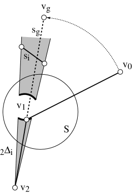
   Figure 3: The triangle cone ${}_{2}{\triangle}_{i}$ intersects the sphere $S$ in at most two circular arcs.

   Not every $v_{1}\in{{}_{2}{\triangle}_{i}}$ leads to intersection of $s_{g}$ with $s_{i}$: $s_{g}$ must reach $s_{i}$. The relevant subset of ${{}_{2}{\triangle}_{i}}$ could be detailed, but because it has one curved edge, we content ourselves with a supset of the obstructions by forbidding $v_{1}$ anywhere in ${{}_{2}{\triangle}_{i}}$.

   Applying Lemma 3 shows that $S\cap{{}_{2}{\triangle}_{i}}$ contributes at most two arcs or points to ${{\rm Ob}(v_{1})}$, for each $i\not\in\{0,1\}$.

2. Intersections between $s_{0}$ and $s_{1}$ and the remainder of the chain. ${{\rm Ob}(v_{1})}$ also contains all the positions of $v_{1}$ that cause the two adjacent links to intersect any of the other segments. The link $v_{2}v_{1}$ is clearly covered by ${}_{2}{\triangle}_{i}$. The link $v_{0}v_{1}$ can be handled by the analogous triangle cone ${}_{0}{\triangle}_{i}$ with apex at $v_{0}$ and through $s_{i}$. Again these sets provide a superset of the obstructions, and Lemma 3 again applies.

Summing over all $i$ yields the obstruction superset ${{\rm Ob}(v_{1})}$ composed of at most $2\cdot 3(n-2)=O(n)$ arcs or points on $S$. Thus ${{\rm Ob}(v_{1})}$ is an arrangement of $O(n)$ arcs on a $2$-sphere, with the initial position of $v_{1}$ lying on at least one arc (because by hypothesis, $s_{g}$ is intersected). Choosing any point $v^{\prime}_{1}\in S\setminus{{\rm Ob}(v_{1})}$ interior to an arrangement cell on whose boundary $v_{1}$ lies suffices to establish the claim. $\Box$

Note that it is quite possible for $v_{1}$ to be confined within a cell of the arrangement ${{\rm Ob}(v_{1})}$, but that this “cage” is no impediment. We do not need a path from $v_{1}$ to an arbitrary point of $S$; rather we only need a path to any unobstructed point $v^{\prime}_{1}$. Although we could construct the arrangement ${{\rm Ob}(v_{1})}$ in $O(n^{2}\alpha(n))$ time and $O(n^{2})$ space [EGP⁺92, Hal97], for our limited goal of constructing just one point, we can do better:

Lemma 8

A move of $v_{1}$ to the position guaranteed by Lemma 7 may be computed in $O(n)$ time and $O(n)$ space.

Proof: Let $Z=\{a_{1},\ldots,a_{m}\}$ be the collection of arcs of $V$ that contain $v_{1}$. $Z$ may be found by a brute force check of each of the $O(n)$ arcs. Pick two arcs $a_{1}$ and $a_{j}$ angularly consecutive about $v_{1}$. This can be accomplished in $O(n)$ time by fixing $a_{1}$, and letting $a_{j}$ be the arc that makes the smallest angle with $a_{1}$. Let $a$ be a circular arc ray (i.e., a directed great circle starting and ending at $v_{1}$) that bisects this angle; or if $Z$ only contains one arc, let $a$ be orthogonal to it; or if $Z$ only contains one point, let $a$ be any ray from $v_{1}$.

Intersect $a$ with every arc and point of ${{\rm Ob}(v_{1})}$, again in $O(n)$ time. Let ${\delta}$ be the distance from $v_{1}$ along $a$ to the closest intersection. Finally, choose $v^{\prime}_{1}$ as the point ${\delta}/2$ along $a$. This point is guaranteed to be off ${{\rm Ob}(v_{1})}$, and therefore unobstructed.

Moving (in one move) $v_{1}$ to $v^{\prime}_{1}$ establishes a new goal $s^{\prime}_{g}$ that is not intersected. $\Box$

2.1.3 Motion Planning

Now that we know we can perform Step 2 of Algorithm 1a in $O(n)$ time per iteration, we return to finding a path through $S^{3}$ for $v_{0}$, as guaranteed by Lemma 6. Motion planning between two points of the $3$-sphere ${\cal{F}}$ may be achieved by any general motion planning algorithm [Sha97, Sec. 40.1.1]. For example, Canny’s Roadmap algorithm achieves a time and space complexity of $O(n^{k}\log n)$, where $n$ is the number of obstacles, and $k$ the number of degrees of freedom in the robot’s placements. In our case, $k=3$. His algorithm produces a piecewise algebraic path through ${\cal{F}}$, of $O(n^{k})$ pieces. Each piece constitutes a constant number of moves, with the constant depending on the algebraic degree of the curves, which is bounded as a function of $k$. Therefore each joint straightening can be accomplished in $O(n^{3})$ moves. Repeating the planning and straightening $n$ times leads to $O(n^{4})$ moves in $O(n^{4}\log n)$ time. In the next section we reduce the $O(n^{3})$ moves per joint straightening to just $3$ moves per straightening.

2.2 Algorithm 1b

We have now established Theorem 1, but with weaker complexity bounds than claimed. It is not surprising that applying a general motion planning algorithm is wasteful in our relatively simple situation. In fact a significant improvement over Algorithm 1a can be achieved by switching attention from the absolute position of $v_{0}$, to the direction in which $s_{0}$ rotates. Let the vector along $s_{0}$ be $w_{0}=v_{0}-v_{1}$, and similarly let $w_{g}=v_{g}-v_{1}$. Let $w$ be the goal direction: a unit vector orthogonal to $w_{g}$ that represents the direction in which $w_{0}$ should be rotated to move it to its goal position. See Fig. 4.

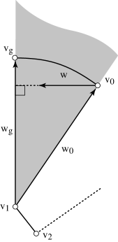
Figure 4: The goal direction vector $w$ defines the direction that $w_{0}$ should be rotated to reach $w_{g}$. The shaded triangle cone ${{}_{1}{\triangle}(v_{0},v_{g})}$ is not crossed by any links of the chain if $w$ is unobstructed.

Thus $w$ is the unique unit vector pointing in the direction of the component of $w_{g}-w_{0}$ orthogonal to $w_{g}$:

$$a_{1}w_{g}+b_{1}w=w_{g}-w_{0}$$ (7)

for some reals $a_{1}>0$ and $b_{1}>0$. The space of possible directions $w$ forms a $2$-sphere rather than the $3$-sphere we faced in Step 1 of Algorithm 1a. This permits replacing the $O(n^{3}\log n)$ moves per step from motion planning, with at most two moves. We now proceed to describe this. Because this represents a computational improvement only, the proofs are only sketched. More detailed proofs are contained in [Coc99].

Algorithm 1b distinguishes three possibilities:

1. The goal position is intersected by some other link of the chain (just as in Algorithm 1a).

2. The goal direction is obstructed in that rotation of $s_{0}$ in the direction $w$ might hit some link of the chain along its direct rotation to the goal position. We again define a direction to be obstructed conservatively, working with a superset of the true obstructions: $w$ is obstructed if the triangular cone ${\triangle}_{v_{1}}(v_{0},v_{g})={{}_{1}{\triangle}(v_{0},v_{g})}$ is intersected by any $s_{i}$, $i>1$.

3. The goal direction is free: it is not obstructed (and so the goal position is not intersected).

A high-level view of our second algorithm is as follows:

Algorithm 1b: Open Chains repeat until chain straightened do 1: if $w$ is free then Rotate $s_{0}$ directly to $s_{g}$. 2: else if $w$ is obstructed then Rotate $s_{0}$ to new position whose goal direction is free. 3: else if $s_{g}$ is intersected then Move $v_{1}$ so that the goal position is not intersected.

Step 3 is identical to Step 2 of Algorithm 1a, so we only discuss the first two steps.

2.2.1 Step 1: $w$ is free

By our definitions, $s_{0}$ may be rotated directly to $s_{g}$ without hitting any other segment of the chain. Because the goal position $s_{g}$ is not intersected, the chain remains simple even after the rotation has been completed. Therefore, the link $s_{0}$ can be straightened in one move.

Note that this is the generic situation, in that for a “random” chain, e.g., one whose vertex coordinates are chosen randomly from a 4D box, each link can be straightened with Step 1 of the algorithm with probability $1$. Steps 2 and 3 handle “degenerate” cases. We exploit this in our implementation (Section 2.3).

2.2.2 Step 2: $w$ is obstructed (but $s_{g}$ is not intersected)

Detecting obstructions.

When $w$ is obstructed, we again rely on construction of an obstruction diagram. First we describe the space in which the obstruction diagram is embedded.

Consider the space of possible directions from which $s_{0}$ might approach $s_{g}$. In 3D, this set of unit vectors forms a $1$-sphere, a circle, which can be viewed as orthogonal to $s_{g}$ and centered at $v_{g}$; see Fig. 5a. Similarly, in 4D, the set of possible approach directions toward $s_{g}$ forms a unit $2$-sphere $S$, which again we center on $v_{g}$. Every point on this sphere represents a direction of approach to $s_{g}$; see Fig. 5b.

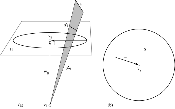
Figure 5: (a) Directions approaching the goal position in 3D; (b) $S$ is a $2$-sphere in $\mathbb{R}^{4}$.

The obstruction diagram Ob$(s_{g})$ is the set of vectors $w$ representing obstructed goal directions for $s_{g}$.

Lemma 9

If the goal $s_{g}$ is not intersected, the obstruction diagram Ob$(s_{g})$ consists of at most $n$ arcs on $S$.

Proof: Take an arbitrary segment $s_{i}$ of the chain, and “project” it to $s^{\prime}_{i}$ in the $3$-flat $\Pi\supset S$ orthogonal to $s_{g}$; i.e., $s^{\prime}_{i}={{}_{1}{\triangle}_{i}}\cap\Pi$. See Fig. 5a for the 3D analog. We first claim that the set of directions $w$ obstructed by $s^{\prime}_{i}$ is identical to those obstructed by $s_{i}$. Next we determine this set of directions. Every vector $w$ determined by a point on $S$ and its center $v_{g}$, is orthogonal to $s_{g}$ by our choice of $\Pi$. So the set of $w$ obstructed by $s^{\prime}_{i}$ is just those $w$ determined by the intersection of ${{}_{g}{\triangle}}(s^{\prime}_{i})$ with $S$. By Lemma 3, this is at most one arc on the sphere. See Fig. 6.

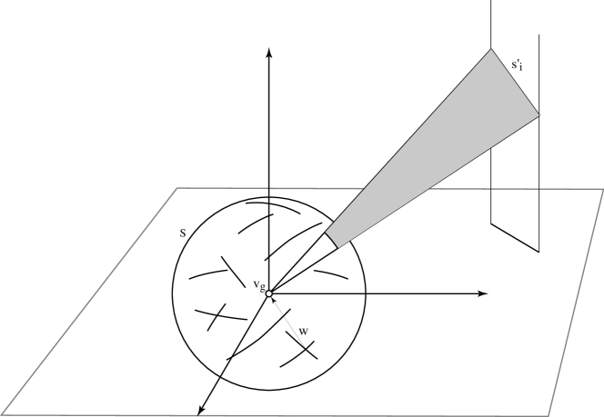
Figure 6: In 4D, $s_{i}$ projects to $s_{i}^{\prime}$ in the $3$-flat containing $S$, and produces an arc of the obstruction diagram determined by the intersection of the triangle cone ${{}_{g}{\triangle}}(s^{\prime}_{i})$ with $S$.

$\Box$

Detection of obstruction therefore reduces to deciding if $w$ lies on one or more arcs of an arrangement of circular arcs on a $2$-sphere $S$, which can be accomplished in $O(n)$ time and space as in Lemma 8.

Skirting obstructions.

Our next task is to move $s_{0}$ when $w$ is obstructed so that its new goal direction is free. This task is similar to that handled in Lemma 8—stepping off the arcs meeting at $w$—with one additional constraint: the move must maintain the simplicity of the chain. Note that Ob$(s_{g})$ does not record chain simplicity, but rather records free goal directions. So we need to find a $\Delta w$ that will move $w$ to be free, while simultaneously maintaining simplicity during the motion of $s_{0}$.

Lemma 10

If $w$ is obstructed, $s_{0}$ can be moved, maintaining simplicity throughout, so that its new goal direction $w^{\prime}=w+\Delta w$ is unobstructed. $\Delta w$ may be computed in $O(n)$ time and space.

Proof: Because the chain is initially simple, there must exist a ${\beta}>0$ such that rotation of $s_{0}$ about $v_{1}$ by an angle less than ${\beta}$ leaves the chain simple. This ${\beta}$ can be computed by finding the smallest distance $d$ from $s_{0}$ to any other segment, and using the angle of a cone centered at $s_{0}$ of radius $d/2$. Now $\Delta w$ is selected just as in Lemma 8, but subject to this angle constraint. $\Box$

Note that because we have based our analysis on a fixed $s_{g}$, moving $s_{0}$ does not alter the obstruction diagram, which records obstructed directions of approach to $s_{g}$.

2.2.3 Algorithm 1b Complexity

The algorithm straightens one joint in at most three moves: one to move $v_{1}$ so the goal is not intersected (Step 3), one to move $v_{0}$ so that the goal is not obstructed (Step 2), and one to rotate directly to the goal (Step 1). The total number of moves used by the algorithm is then at most $3n=O(n)$. For each of the $n$ iterations, Lemma 10 shows that the computations can be performed in linear time and space. This then establishes the total time complexity of $O(n^{2})$ claimed in Theorem 1. Because each move is performed independently, the obstruction diagram arcs may be discarded after each iteration. Thus the space requirements remain at $O(n)$.

2.3 Implementation

We have implemented Algorithm 1b for chains in “general position” in C++. The program accepts a chain as input, and first checks if it is simple. If it is, the straightening process starts; otherwise the program exits. The program then straightens the chain link-by-link using Step 1, one move per link. It also detects whether the goal is obstructed (Step 2) or intersected (Step 3) by solving sets of linear equations, but in those cases it simply halts; we have not implemented the obstruction diagrams, or avoiding obstructions. For a chain whose vertex coordinates are chosen randomly, the program straightens it with probability $1$, for then the degenerate cases handled by Steps 2 and 3 (when a point, $w$ or $v_{1}$, hits an arc on a $2$-sphere, e.g., Fig. 6) are unlikely to occur. The output of the program is a set of Geomview or Postscript files that animate the straightening process. Fig. 7 shows output for a chain whose $n=100$ vertices were chosen randomly and uniformly in $[0,1]^{4}$.

Figure 7: Snapshots of the algorithm straightening a chain of $n=100$ vertices, initially $(0)$, and after $25$, $50$, $75$, and all $99$ joints have been straightened (left to right). (a) Scale approx. 50:1; the entire chain is visible in each frame. (b) Scale approx. 1:1; the straightened tail is “off-screen.” (The apparent link length changes are an artifact of the orthographic projection of the 4D chain down to 2D.)

3 Straightening Trees in 4D

It will come as no surprise that essentially the same algorithm as just described can straighten trees in 4D. The reason is that each segment was considered a fixed obstruction in the chain straightening algorithm, and whether those segments form a chain or a tree is largely irrelevant, as long as there is a free end. There is one spot at which the difference between a chain and a tree does matter, however: freeing up an intersected goal position. We concentrate on this difference in the description below.

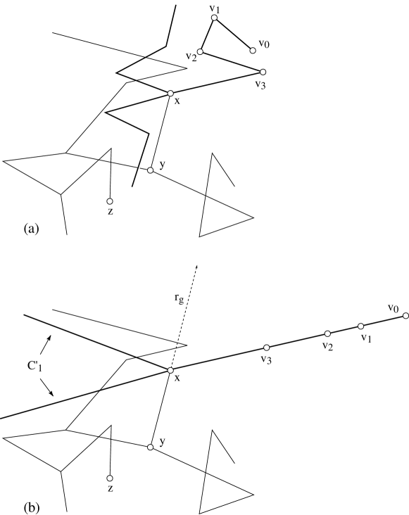
Figure 8: (a) Tree $T$ rooted at $z$; (b) After straightening chains $C$ incident to $x$; $C^{\prime}_{1}$ is the set of straightened chains excluding one distinguished chain $(v_{0},v_{1},\ldots)$.

Algorithm 2: Trees repeat until straightened do 1: Identify a node $x$ with chain descendants $C$. 2: Straighten each chain in $C$, forming $C^{\prime}$. 3: if $r_{g}$ is intersected then Construct obstruction diagram Ob$(x)$ on 2-sphere. Move $x$ so that $r_{g}$ not intersected. 4: Rotate each segment in $C^{\prime}$ to $r_{g}$ and coalesce.

Algorithm 2 chooses a leaf $z$ of the given tree $T$ as root, and then identifies some node $x$ all of whose descendant subtrees are chains (Step 1). Call this set $C$; see Fig. 8a. Each chain in $C$ can be straightened one at a time via Algorithm 1, leaving a set of straightened chains, or segments, $C^{\prime}$ (Step 2). Define the goal ray to be the extension of the parent segment $yx$ incident to $x$; see Fig. 8b. If $r_{g}$ is not intersected by any segment of $T\setminus C^{\prime}$, then each segment in $C^{\prime}$ can be rotated to $r_{g}$, each lying on top of one another (Step 4). We can view them as coalesced into a single link, reducing the degree of $x$ to $2$. The process then repeats.

If, however, $r_{g}$ is intersected (Step 3), we need to move $x$ so that the goal ray becomes free. There are several ways to achieve this; we choose to parallel Step 2 of Algorithm 1a. Let $(v_{0},v_{1},\ldots,v_{m})$ be one of the chains of $C^{\prime}$, with $v_{m}$ adjacent to $x$. We distinguish this chain from the others in $C^{\prime}$; call the set of others $C^{\prime}_{1}$. Let the $2$-link chain $(v_{0},x,y)$ play the role of $(v_{0},v_{1},v_{2})$ in Algorithm 1a. In that algorithm we argued that Ob$(v_{1})$ is a set of arcs and points on a $2$-sphere (Fig. 3). Here will will reach the same conclusion for Ob$(x)$ on the $2$-sphere $S$ of positions for $x$.

The only difference is that in the current situation, the star of segments $C^{\prime}_{1}$ is attached to $x$, and we need to augment Ob$(x)$ to reflect its obstructions. We opt to translate $C^{\prime}_{1}$ as $x$ moves; this gives rise to two sets of constraints: (1) those caused by a segment in $C^{\prime}_{1}$ intersecting a segment of $T^{\prime}=T\setminus\{C^{\prime}_{1}\cup xy\cup xv_{0}\}$; (2) those caused by $xy$ or $xv_{0}$ intersecting a segment in $C^{\prime}_{1}$. For the first, the locus of positions of $x$ that cause some $s\in C^{\prime}_{1}$ to intersect some $s_{i}\in T^{\prime}$ is a parallelogram, congruent to the Minkowski sum $s\oplus s_{i}$. Analogous to Lemma 3, it is easy to see that this holds:

Lemma 11

The intersection of a parallelogram with a $(d{-}1)$-sphere $S$ in $\mathbb{R}^{d}$ consists of at most four connected components, each of which is an arc or a point.

$\Box$

Thus the constraints (1) add $O(n)$ arcs or points to Ob$(x)$. Constraints (2) can be seen to consist of $O(n)$ points on $S$: translating the star $C^{\prime}_{1}$ to $y$ determines the rays that $xy$ might align with to cause $xy$ to intersect $C^{\prime}_{1}$; and similarly translating $C^{\prime}_{1}$ to $v_{0}$ determines rays for intersection with $xv_{0}$. The two placements of $C^{\prime}_{1}$ therefore generate $O(n)$ additional point obstructions.

With Ob$(x)$ again a set of $O(n)$ arcs and points on a $2$-sphere, Lemmas 7 and 8 hold, leading to the same time complexities clamed for Algorithm 1, and establishing Theorem 2.

4 Convexifying Closed Chains in 4D

Our algorithm for convexifying closed chains employs the line tracking motions introduced in [LW95]. Indeed our algorithm mimics theirs in that we repeatedly apply line tracking motions, each of which straightens at least one joint, until a triangle is obtained (which is a planar convex polygon, as desired). Although the overall design of our algorithm is identical, the details are quite different, for there is a major difference with [LW95]: They permitted self-intersections of the chain, whereas we do not. This greatly complicates our task.

Let $(v_{0},v_{1},v_{2},v_{3},v_{4})$ be five consecutive vertices of a closed polygonal chain. We allow $v_{0}=v_{4}$. A line tracking motion of $v_{2}$ moves $v_{2}$ along some line $L$ in space, while keeping both $v_{0}$ and $v_{4}$ fixed. As long as the angle at joints $v_{1}$ and $v_{3}$ (the elbows) are neither $\pi$ (straight) nor $0$ (folded), such a motion is possible. Neither angle can be $0$ because that would violate the simplicity of the chain. Straightening one joint is precisely our goal, so we assume that neither joint is straight; and therefore a line tracking motion is possible.

We will choose $L$ and a direction along it so that the movement increases the distance from $v_{2}$ to both $v_{0}$ and $v_{4}$ simultaneously. This necessarily opens both elbow angles. The motion stops when one elbow straightens. The only issue is whether this can be done while maintaining simplicity. Our aim is to prove this theorem:

Theorem 6

For a simple 4D chain $(v_{0},\ldots,v_{4})$, there exists a line tracking motion of $v_{2}$ that straightens either $v_{1}$ or $v_{3}$ (or both) while maintaining simplicity of the chain throughout the motion.

A high-level view of the algorithm is as follows:

Algorithm 3: Closed Chains repeat until chain is a triangle do Compute a line $L$ along which to move $v_{2}$. Compute free paths $\pi_{1}$ and $\pi_{3}$ for $v_{1}$ and $v_{3}$. Move $v_{2}$ along $L$, $v_{1}$ along $\pi_{1}$, and $v_{2}$ along $\pi_{2}$. Freeze the straightened joint $v_{1}$ or $v_{3}$.

4.1 Choosing $L$

To fix $L$, the ray along which $v_{2}$ moves, we choose a point $q\in\mathbb{R}^{4}$ different from $v_{2}$, and let $L$ be the ray from $v_{2}$ that contains $v_{2}q$. We will choose $q$ so that it is itself the point where one of the two joints $v_{1}$ or $v_{3}$ becomes straight while moving $v_{2}$ along $L$.

Lemma 12

A point $q$ determining an appropriate $L$ may always be found, and in time and space $O(n^{4})$.

Proof: We choose $q$ so that it satisfies these conditions:

1. Moving $v_{2}$ along $L$ increases the distance from $v_{2}$ to $v_{0}$ and to $v_{4}$.

2. Either $v_{1}$ or $v_{3}$ becomes straight, i.e., $|qv_{0}|=|v_{0}v_{1}|+|v_{1}v_{2}|=r_{0}$, or $|qv_{4}|=|v_{2}v_{3}|+|v_{3}v_{4}|=r_{4}$

3. 1. If $|qv_{0}|=r_{0}$, then $qv_{0}$ does not intersect any other segment of the chain than those to which it is incident.

   2. If $|qv_{4}|=r_{4}$, then $qv_{4}$ does not intersect any other segment of the chain than those to which it is incident.

4. $v_{2}q$ does not intersect a segment $s_{i}$, $i>4$.

Condition 3 ensures that our “goal” is not itself intersected, in the sense used in Section 2.

Let $R_{i}$ be the set of points (the “region”) of $\mathbb{R}^{4}$ that satisfy Condition $i$ above. $R_{1}$ is the intersection of two closed half-spaces containing $v_{2}$, orthogonal to $v_{0}v_{2}$ and $v_{2}v_{4}$ respectively. Note that $v_{2}\in R_{1}$. If $v_{0}v_{2}$ and $v_{2}v_{4}$ lie on the same line, $R_{1}$ degenerates to a $3$-flat orthogonal to that line; otherwise it is a $4$-dimensional set. See Fig. 9 for a lower dimensional analog of the situation.

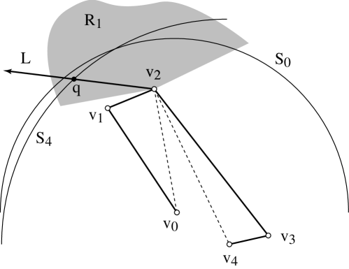
Figure 9: Choosing $q\in L$. $R_{1}\cap R_{2}=R_{1}\cap(S_{0}\cup S_{4})$.

The set of points $R_{2}=S_{0}\cup S_{4}$ in 4D that satisfy Condition 2 is the union of two 3-spheres, $S_{0}$ and $S_{4}$, centered at $v_{0}$ and $v_{4}$ and of radius $r_{0}$ and $r_{4}$, respectively. Because $|v_{0}v_{2}|<r_{0}$, $v_{2}$ is inside the $4$-ball bounded by $S_{0}$. Therefore, $R_{1}\cap S_{0}\neq\emptyset$. Similarly, $R_{1}\mathbb{R}^{4}\setminus\cap S_{4}\neq\emptyset$. So $R_{1}\cap R_{2}\neq\emptyset$. The dimensionality of this set depends on whether or not $\{v_{0},v_{2},v_{4}\}$ are collinear: if they are, the $3$-spheres are intersected by a $3$-flat producing $2$-spheres; if they are not, the $3$-spheres are intersected by a $4$-dimensional wedge, producing $3$-dimensional regions of the $3$-spheres.

Consider Condition 3a; clearly 3b is analogous. We want all those points $q$ such that $qv_{0}$ does not intersect any other link of the chain. Clearly the points forbidden by segment $s_{i}$ lie in the triangle cone ${{}_{0}{\triangle}_{i}}={\triangle}_{v_{0}}(v_{i},v_{i+1})$, just as in the proof of Lemma 7. Intersecting ${{}_{0}{\triangle}_{i}}$ for all $i$ with $R_{1}\cap R_{2}$ marks the set of points that must be avoided in our choice of $q$: $R_{3}\supset\mathbb{R}^{4}\setminus\bigcup_{i}{{}_{0}{\triangle}_{i}}$. It is easiest to concentrate on the intersection of ${}_{0}{\triangle}_{i}$ with the spheres in $R_{2}$. By Lemma 3, we know this intersection is at most two arcs or points, independent of the dimension of the spheres. So whether or not $\{v_{0},v_{2},v_{4}\}$ are collinear, the intersection produces $O(n)$ arcs or points. Similarly, Condition 4 leads to $R_{4}\supset\mathbb{R}^{4}\setminus\bigcup_{i>4}{{}_{2}{\triangle}_{i}}$, for $v_{2}q$ can intersect $s_{i}$ only if $q$ lies in ${{}_{2}{\triangle}_{i}}$. Again, $O(n)$ arcs or points need be avoided in $R_{1}\cap R_{2}$. No union of arcs and points can cover the set $R_{1}\cap R_{2}$, which is either $2$- or $3$-dimensional. Thus $\bigcap_{i}R_{i}\neq\emptyset$. We need only choose a $q$ in this set.

There are a variety of ways to choose such a $q$ algorithmically. A naive method is to first construct an arrangement of $2$-flats in $\mathbb{R}^{4}$ each containing a triangle ${}_{0}{\triangle}_{i}$ or ${}_{2}{\triangle}_{i}$. This computation could be performed in $O(n^{4})$ time and space [ESS93]. Intersecting this arrangement with the halfspaces delimiting $R_{1}$ and the $3$-spheres $S_{0}$ and $S_{4}$ leave us cells bound by algebraic surfaces inside $\bigcap_{i}R_{i}$. The centroid of any such cell can be selected as $q$. $\Box$

4.2 Line Tracking in 3D

We start by thinking about the analogous situation in 3D. This will both set notation, and ground intuition by showing why Theorem 6 does not hold in 3D.

4.2.1 Topology of Configuration Space in 3D

Let $\mathbb{R}_{[0,1)}$ be the interval $[0,1)$ on the real line, open at $1$. We will parametrize the location of $v_{2}$ along $L$ by $t\in[0,1)$, with $t=0$ the start, and $t=1$ when $v_{2}$ reaches the $q$ of Lemma 12, the first time at which a joint, straightens. Let this joint be $v_{1}$ without loss of generality. Let ${\cal{C}}^{\prime}$ be the configuration space of the four-link system in isolation, permitting intersections between the links, the prime to remind us that $t=1$ has been excluded. We claim that

$${\cal{C}}^{\prime}=\mathbb{S}^{1}\times\mathbb{S}^{1}\times\mathbb{R}_{[0,1)}.$$ (8)

This can be seen as follows. Fix some $t$ so that $v_{2}$ is fixed. Then each of $v_{1}$ and $v_{3}$ is free to rotate (independently) on a circle in $\mathbb{R}^{3}$ centered on the axis $v_{0}v_{2}$ and $v_{2}v_{4}$ respectively. As $t$ varies from $0$ to $1$, these circles move in space, and grow and shrink in radius; see Fig. 10.

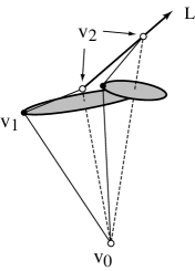
Figure 10: In 3D, the circle on which $v_{1}$ may lie moves in space as $v_{2}$ slides up $L$.

At $t=1$ the $v_{1}$ circle shrinks to a point. But for $t\in[0,1)$, both circles retain a positive radius. Thus the configuration space ${\cal{C}}$ has the topology of $\mathbb{S}^{1}\times\mathbb{S}^{1}$ for each $t$, and the claim follows.

4.2.2 Obstruction Diagram in 3D

As in Section 2, we incorporate the obstacles representing the other links via an “obstruction diagram.” We start by ignoring the four moving links as obstructions, and only consider the remaining, fixed links of the polygonal chain as obstacles. We develop the obstruction diagram first for fixed $t$, so that the relevant configuration space is $\mathbb{S}^{1}\times\mathbb{S}^{1}$. Because we are ignoring the moving links as obstructions, movement on the two circles is independent, so it suffices to determine the obstruction diagram Ob$(v_{1})$ on one $1$-sphere/circle $S_{1}$, that for $v_{1}$. The following lemma will be key in 4D:

Lemma 13

In 3D, if $(v_{2}-v_{0})\cdot(v_{1}-v_{0})\neq 0$ and $(v_{2}-v_{0})\cdot(v_{1}-v_{2})\neq 0$, then a single segment contributes at most four points to Ob$(v_{1})$. Otherwise, if either dot product is zero, a segment could obstruct a finite-length arc of the $S_{1}$ circle for $v_{1}$.

Proof: We only sketch a proof, leaving details for the 4D case considered below. Spinning $v_{1}$ along its circle of freedom while maintaining $v_{0}$ and $v_{2}$ fixed traces out a “spindle” shape, which can be viewed as the union of two cones. A segment $s$ that does not lie along a line through either $v_{0}$ or $v_{2}$ can intersect each cone in at most two points, and so intersect the spindle in at most four points. See Fig. 12.

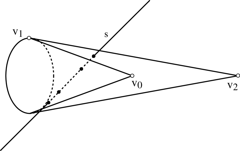
Figure 11: One segment $s$ can contribute four points to Ob$(v_{1})$.

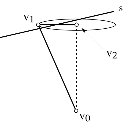
Figure 12: $(v_{2}-v_{0})\cdot(v_{1}-v_{2})=0$ and segment $s$ (which lies in the plane of the circle) contributes an arc to the obstruction diagram Ob$(v_{1})$.

These four segment-cone intersection points correspond one-to-one with four $v_{1}$ positions on $S_{1}$ at which there is an intersection between the $2$-link chain $(v_{0},v_{1},v_{2})$ and $s$.

If the segment $s$ lies in the surface of the cone, then it contributes just one point to the diagram, corresponding to the angle of spin that aligns one of the two links with the obstacle segment.

Finally, if either of the two links $v_{0}v_{1}$ or $v_{1}v_{2}$ is orthogonal to the axis of the spindle, i.e., either dot product is zero, then a segment obstacle could obstruct the entire circle, for one of the cones is then degenerately flat. As Fig. 12 illustrates, here a segment might obstruct a range of rotations of $v_{1}-v_{2}$, producing an arc in Ob$(v_{1})$. $\Box$

4.2.3 Disconnected Free Space in 3D

Let $v_{1}(t)$ represent the position of $v_{1}$ on its circle $S_{1}$ at a particular time $t$. The goal is for the links $(v_{0},v_{1},v_{2})$ to avoid all obstacles, which means that $v_{1}(t)$ should avoid points of the obstruction diagram. If we ignore for now the orthogonality case, then we have the situation that a finite set of links produce an obstruction diagram consisting of a finite set of points on $S_{1}$. As $t$ moves, these points wander around the circle, disappear, enter, join, or split. The moving links, previously ignored, just add a few more points to the obstruction diagram, moving in a different manner. The diagram for the configuration space for $v_{1}$ then looks like arcs on the tube-like $\mathbb{S}\times\mathbb{R}_{[0,1)}$. It is clear that it is possible for the point $v_{1}(t)$ to be “captured” between two points of the obstruction diagram which move together and squeeze $v_{1}(t)$ into a collision. See Fig. 13. In this case, the free space for the point $v_{1}$ is not connected from $p_{1}(0)$ to $p_{1}(1)$.

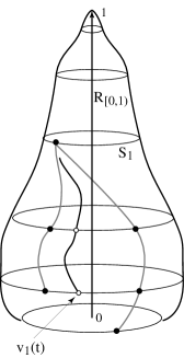
Figure 13: Point $v_{1}(t)$ is “captured” by two obstacle points in configuration space, the tube-like surface.

And indeed it is easy to “cage in” the moving links by the fixed links so that no straightening is possible. Our next task is to show that such caging-in is impossible in 4D.

4.3 Line Tracking in 4D

4.3.1 Topology of Configuration Space in 4D

Turning now to 4D, exactly analogous to the situation in 3D, an elbow at the join of two links has a space of possible motions in 4D that is topologically $\mathbb{S}^{2}$, for it is the intersection of two 3-spheres. Thus the configuration space ${\cal{C}}^{\prime}$ of our four-link chain for $t\in[0,1)$, ignoring self-intersections, is

$${\cal{C}}^{\prime}=\mathbb{S}^{2}\times\mathbb{S}^{2}\times\mathbb{R}_{[0,1)}\;.$$ (9)

At $t=1$ at least one of the $2$-spheres shrinks to a point.

4.3.2 Obstruction Diagram in 4D

As in 3D, we analyze the obstruction diagram on one $2$-sphere $S_{1}$, that for $v_{1}$, at a fixed value of $t$: Ob$(v_{1})$. Let $v_{1}(t)$ represent the position of $v_{1}$ on its sphere $S_{1}$ at time $t$. We seek the set of points Ob$(v_{1})$ for which the links $(v_{0},v_{1},v_{2})$ intersect some other segment of the chain, $s_{4},s_{5},\ldots,s_{n}$. Just as in 3D, Ob$(v_{1})$ is (in nondegenerate situations) a finite set of points. This claim relies on how a line may intersect a cone.

Define a $(d{-}1)$-cone $C(a,b,{\theta})$, for apex point $a$, axis point $b$, and cone angle ${\theta}\in[0,\pi/2]$, to be the set of points $p\in\mathbb{R}^{d}$ that form an angle ${\theta}$ with respect to the axis, i.e., which satisfy:

$$(p-a)\cdot(b-a)=|p-a||b-a|\cos{\theta}\;.$$ (10)

For the extreme values of ${\theta}$, $C(a,b,0)$ is a ray from $a$ through $b$, and $C(a,b,\pi/2)$ is a $(d{-}1)$-flat containing $a$ and orthogonal to $ab$. Note that a $1$-cone is not the triangle cone from Section 2.1.1; rather a $1$-cone is the union of two rays from $a$. In 3D, $C(a,b,{\theta})$ is the surface of a right circular cone whose axis is the ray from $a$ through $b$, and which form the angle ${\theta}$ with the axis at $a$ (cf. Fig. 12). Its intersection with a plane orthogonal to $ab$ is a circle. In 4D, $C(a,b,{\theta})$ is a “right spherical cone,” whose intersection with a $3$-flat orthogonal to $ab$ is a $2$-sphere. Note that it is no restriction to insist that ${\theta}\in[0,\pi/2]$, for we can ensure this for ${\theta}>\pi/2$ by selecting an axis point $b^{\prime}$ for the cone to be on the other side of the apex $a$, on the line containing $ab$, thereby “reflecting” ${\theta}$ to $\pi-{\theta}$.

Lemma 14

The intersection of the $(d{-}1)$-cone $C(a,b,{\theta})$, ${\theta}\neq\pi/2$, with a line, ray, or segment whose containing line does not include the apex $a$, is at most two points: two points, one point, or empty.

This claim can be seen intuitively as follows. Let $C$ be the cone and $s$ a segment in $\mathbb{R}^{d}$. If $s$ is contained in a $(d{-}1)$-flat $\Pi$ orthogonal to $ab$, then because $\Pi\cap C$ is a sphere, the result follows from Lemma 2. Otherwise $s$ is contained in a flat whose intersection with $C$ is an ellipsoid, and the result follows because an ellipsoid is affinely equivalent to a sphere [Sam88, p. 95].

Proof: Let $|ab|=1$ without loss of generality. Translate and rotate $C$ so that $a=(0,0,\ldots,0)$ and $b=(1,0,0,0,\ldots,0)$. For a point $p=(x_{1},\ldots,x_{d})$, Eq. (10) reduces to

$$p\cdot b = |p|\cos{\theta}$$ (11)

$$(x_{1},\ldots,x_{d})\cdot(1,0,0,0,\ldots,0) = \sqrt{x_{1}^{2}+\cdots+x_{d}^{2}}\cos{\theta}$$ (12)

$$x_{1}^{2} = (x_{1}^{2}+\cdots+x_{d}^{2})\cos^{2}{\theta}$$ (13)

Represent the point $p$ via the parameter $t$:

$$p=({\alpha}_{1}+{\beta}_{1}t,\ldots,{\alpha}_{d}+{\beta}_{d}t)\;.$$ (14)

Substitution of this into Eq. (13) yields a quadratic equation in $t$, which has at most two roots.

We now examine the degenerate solutions. Because we assumed that ${\theta}\neq\pi/2$, $\cos{\theta}\neq 0$. Thus the righthand side of Eq. (13) can only be zero when $x_{1}^{2}+\cdots+x_{d}^{2}=0$, i.e., when $p=(0,0,\ldots,0)$ is the apex $a$. This corresponds to a line through $a$, excluded by our assumptions. $\Box$

Lemma 15

In 4D, if $(v_{2}-v_{0})\cdot(v_{1}-v_{0})\neq 0$ and $(v_{2}-v_{0})\cdot(v_{1}-v_{2})\neq 0$, then a single segment $s$ contributes at most four points to Ob$(v_{1})$.

Proof: Moving $v_{1}$ sweeps out two finite cones, which are truncations of the infinite cones $C(v_{0},v_{2},{\theta}_{0})$ and $C(v_{2},v_{0},{\theta}_{2})$, with

$$(v_{2}-v_{0})\cdot(v_{1}-v_{0})=|v_{2}-v_{0}||v_{1}-v_{0}|\cos{\theta}_{0}$$ (15)

$$(v_{2}-v_{0})\cdot(v_{1}-v_{2})=|v_{2}-v_{0}||v_{1}-v_{2}|\cos{\theta}_{2}$$ (16)

By the preconditions of the lemma, we have ${\theta}_{j}\neq\pi/2$, $j=0,2$, so we may assume ${\theta}_{j}\in[0,\pi/2)$ by the reflection maneuver suggested previously. Consider two cases:

1. The line containing $s$ does not pass through either cone apex, $v_{0}$ or $v_{2}$. The conditions of Lemma 14 are satisfied, establishing that $s$ intersects the two cones in at most four points. Each of these points fixes a position of $v_{1}$ corresponding to an obstruction, and so contributes this point to Ob$(v_{1})$.

2. The line $H$ containing $s$ passes through $v_{0}$ (the case through $v_{2}$ is exactly analogous and will not be treated separately). Then it may be that $s\cap C(v_{0},v_{2},{\theta}_{0})$ is a subsegment of $s$. This is because the vector $p-v_{0}$ makes the same angle with $v_{2}-v_{0}$ for all $p\in s$ (cf. Eq. (10)). In this case, $s$ obstructs the unique position of $v_{1}$ that places it on $H$, and so contributes just one point to Ob$(v_{1})$. Together with the at most two points from the other cone, $s$ generates at most three points of Ob$(v_{1})$.

$\Box$

The case excluded by the precondition of Lemma 15 refers to the situation in which one cone is degenerately flat, as previously illustrated in Fig. 12. We now analyze this situation in detail.

Lemma 16

If $(v_{2}-v_{0})\cdot(v_{1}-v_{0})=0$, then Ob$(v_{1})$ is a finite set of points and arcs on $S_{1}$ (the $2$-sphere of $v_{1}$ positions).

Proof: In this case ${\theta}_{0}=\pi/2$ from Eq. (15), and the infinite cone $C(v_{0},v_{2},\pi/2)$ degenerates to the $3$-flat orthogonal to the axis $v_{0}v_{2}$ and including the apex $v_{0}$. The finite cone swept out by the link $s_{0}=v_{0}v_{1}$ is a ball $B_{0}$ of radius $\ell_{0}$ centered at $v_{0}$. In the 3D situation, $B_{0}$ is a disk (cf. Fig. 12); in 4D, it is a solid sphere whose boundary is a $2$-sphere $S_{1}$ representing the possible positions for $v_{1}$.

The obstructed positions on $S_{1}$ are those for which $s_{0}$ intersects some segment $s_{i}$. Consider two possibilities:

1. $s_{i}$ does not lie in the same $3$-flat of $\mathbb{R}^{4}$ as $S_{1}$. Then $s_{i}$ intersects $B_{0}$ in at most one point $p$ (because it can intersect the flat in at most one point), and then only when $s_{0}$ passes through $p$ do we have an obstruction. Thus $s_{i}$ contributes one point to Ob$(v_{1})$.

2. $s_{i}$ is in the same $3$-flat as $S_{1}$. Now we have a situation exactly analogous to that shown in Fig. 6: the obstruction is the intersection of the triangle cone ${{}_{0}{\triangle}_{i}}$ with $S_{1}$. Lemma 3 then establishes that $s$ adds at most two arcs or points to Ob$(v_{1})$.

$\Box$

Lemma 17

The condition $(v_{2}-v_{0})\cdot(v_{1}-v_{0})=0$ can hold at most one value of $t\in[0,1]$ during the movement of $v_{2}$ along $L$.

Proof: This follows immediately from our choice of $L$, which guarantees that the distance $|v_{0}v_{2}|$ increases, and so the angle at $v_{1}$ opens. This angle can therefore pass through $\pi/2$ at most once. See Fig. 14.

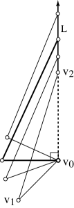
Figure 14: The special condition $(v_{2}-v_{0})\cdot(v_{1}-v_{0})=0$ holds at most once.

$\Box$

4.3.3 Connected Free Space in 4D

Again let $v_{1}(t)$ represent the position of $v_{1}$ on its $2$-sphere $S_{1}$ of possible positions. We first describe the free space for the motion of the $2$-link chain $(v_{0},v_{1},v_{2})$, avoiding the fixed links $s_{4},s_{5},\ldots,s_{n}$. It is a subset of $\mathbb{S}^{2}\times\mathbb{R}_{[0,1)}$. For each $t\in[0,1)$, we know from Lemma 15 that Ob$(v_{1})$ is a set of points or arcs; and from Lemma 17 we know Ob$(v_{1})$ is a finite set of points, except for at most one $t$, at which it is a set of points and arcs. Thus if $v_{1}(t)$ avoids these obstructions, it avoids intersection with the remainder of the chain.

But now it should be clear that it is easy for $v_{1}(t)$ to “run away” from the obstructions. Think of its sphere of possible positions growing and shrinking with time $t$. $v_{1}(t)$ must avoid a set of points at any one time, and once (cf. Lemma 17), a set of arcs. This is easily done: there is no way to “cage” in $v_{1}(t)$ with these obstacles. Another view of this situation is that the configuration space $\mathbb{S}^{2}\times\mathbb{R}_{[0,1)}$ is $3$-dimensional, and the obstructions Ob$(v_{1}(t))$ for $t\in[0,1)$ are $1$- or $0$-dimensional, and the removal of a 1D set cannot disconnect a 3D set (cf. proof of Lemma 6).

The remainder of this subsection establishes this claim more formally. A path in a topological space $X$ is a continuous function $\gamma:[0,1]\rightarrow X$. A space is path-connected if any two of its points can be joined by a path [Arm79]. We first work with the space ${\cal{C}}^{\prime}_{1}$: the positions for $v_{1}$, for $t\in[0,1)$. Later we will add in $t=1$, and positions for $v_{3}$.

Lemma 18

The free space ${\cal{F}}^{\prime}_{1}\subset{\cal{C}}^{\prime}_{1}$ for $v_{1}$ in the configuration space ${\cal{C}}^{\prime}_{1}=\mathbb{S}^{2}\times\mathbb{R}_{[0,1)}$ is path-connected.

Proof: It will help to view our configuration space as follows. The $2$-sphere $S_{1}$ is represented by a flat two-dimensional sheet, and $\mathbb{R}_{[0,1)}$ is represented as a vertical axis. The result is a three-dimensional space, analogous to Fig. 13, that could look as depicted in Fig. 15. The point obstacles Ob$(v_{1})$ become paths monotone with respect to the vertical $t$-axis. At one $t=t_{1}$ we may have arc obstacles as well. We need to show that $v_{1}(0)$ is connected by a path to $v_{1}(t^{\prime})$, for any $t^{\prime}<1$.

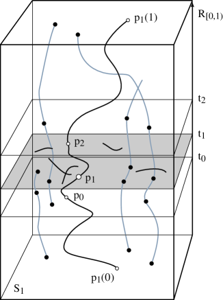
Figure 15: The free space ${\cal{F}}_{1}$ for $v_{1}$ is path-connected. $\pi_{1}$ (dark) connects $p_{1}(0)$ to $p_{1}(1)$. Ob$(v_{1})$ includes points at a fixed $t$, forming curves (shaded) over time. The shaded subspace at time $t=t_{1}$ includes arcs in Ob$(v_{1})$.

We proceed in two cases.

1. Ob$(v_{1})$ contains only points for all $t\in[0,1)$. Let $N$ be the maximum number of points in Ob$(v_{1})$ over all $t$; we know $N\leq 2n$. A $2$-sphere with a finite number $N$ points removed is path-connected. For each $t$, remove $N$ points from the corresponding $S_{1}(t)$: those in Ob$(v_{1})$ at that $t$, and extra distinct points to “pad out” to $N$. Any two spheres with the same number of points removed are homeomorphic. Therefore ${\cal{F}}^{\prime}_{1}$ is homeomorphic to $S_{1}(0)\times\mathbb{R}_{[0,1)}$. Because each of those spaces is path-connected, and the product of two path-connected spaces is path-connected, we have established the claim.

2. Ob$(v_{1})$ contains arcs at $t=t_{1}$. The main idea here is to choose a point $p_{1}=v_{1}(t_{1})$ that is unobstructed at time $t=t_{1}$, and then connect from $v_{1}(0)$ to $p_{1}$, and from $p_{1}$ to $v_{1}(t^{\prime})$. It is clear, as we have shown in Case 1, that the spaces ${\cal{F}}_{-}={\cal{C}}_{/t\in[0,t_{1})}$ and ${\cal{F}}_{+}={\cal{F}}_{/t\in(t_{1},1)}$ are path connected. We will prove that there exist points $p_{0}\in{\cal{F}}_{-}$, and $p_{2}\in{\cal{F}}_{+}$ such that $p_{0}$ and $p_{2}$ are connected by a path.

   We will call a point $p$ free if it does not belong to any obstruction diagram. Let $p_{1}\in S_{1}(t_{1})$ be a free point on $S_{1}$ at $t$. It is clear that such a point exists, since the obstruction diagram is a finite set of arcs and points. It is also clear that there exists a neighborhood $U\subset{\cal{F}}^{\prime}_{1}$ of $p_{1}$ all of whose points are free. Choose $p_{0}\in U$, $p_{0}\in S_{1}(t_{0})$, $t_{0}<t_{1}$ and $p_{2}\in U$, $p_{2}\in S_{1}(t_{2})$, $t_{1}<t_{2}$. See Fig. 15. Both points are free and can be connected by a path in $U$ to $p_{1}$. But $p_{0}\in{\cal{F}}_{-}$ and $p_{2}\in{\cal{F}}_{+}$, both path connected spaces. Thus we may connect $v_{1}(0)$ to $p_{0}$ to $p_{1}$ to $p_{2}$ to $v_{1}(t^{\prime})$.

$\Box$

We now address the endpoint $t=1$, extending $C^{\prime}_{1}$ to $C_{1}$ for $t\in[0,1]$. As $v_{2}$ approaches $q$ on $L$, one of the spheres, that for $v_{1}$ by our assumptions, shrinks to zero radius. Thus Fig. 15 is not an accurate depiction near $t=1$, for the configuration space narrows to a point here.

Lemma 19

The free space ${\cal{F}}_{1}$ for $v_{1}$ in the full configuration space ${\cal{C}}_{1}$ is path-connected.

Proof: We have chosen $q$ and $L$ in Lemma 12 so that the $t=1$ endpoint is free in the sense that the straightened chain $v_{0}v_{1}v_{2}$ does not intersect the fixed portion of the chain. Thus there is a neighborhood $U$ of $t=1$ such that ${\cal{C}}_{1}$ is devoid of all obstructions within that neighborhood. Choose $t^{\prime}\in U$ and apply Lemma 18 to yield a path from $v_{1}(0)$ to $v_{1}(t^{\prime})$. Connect within $U$ from $v_{1}(t^{\prime})$ to the endpoint $v_{1}(1)$. $\Box$

Now we include $v_{3}$ in the analysis.

Lemma 20

The free space ${\cal{F}}\subset{\cal{C}}$ for both $v_{1}$ and $v_{3}$ in the configuration space ${\cal{C}}$ for $t\in[0,1]$ is path-connected.

Proof: The key here is the independence of the motions of $v_{1}$ and $v_{3}$. Let $\pi_{1}$ be a path for $v_{1}(t)$ through ${\cal{F}}_{1}$, whose existence is guaranteed by Lemmas 18 and 19. Now construct ${\cal{F}}_{3}$ as the possible positions $v_{3}(t)$ for $v_{3}$, avoiding at each time Ob$(v_{3}(t))$, where this time the obstructions include not only the fixed links $s_{4},s_{5},\ldots,s_{n}$, but also the two moving links $s_{0}$ and $s_{1}$, determined by $\pi_{1}$. If $v_{3}(t)$ avoids Ob$(v_{3}(t))$ for each $t$, then all intersections are avoided: we do not need to include the moving links in ${\cal{F}}_{1}$, because intersection is symmetric—if the links $s_{2}$ and $s_{3}$ do not intersect $s_{0}$ and $s_{1}$, then $s_{0}$ and $s_{1}$ do not intersect $s_{2}$ and $s_{3}$.

For a fixed $t$, the obstacles are fixed segments, and Ob$(v_{3})$ is again a finite set of points, or, for at most one $t$, a set of arcs: Lemmas 15 and 17 apply unchanged. The independence of the motion of $v_{3}$ from $v_{1}$ permits us to treat the moving segments $s_{0}$ and $s_{1}$ on par with the fixed segments: the only difference is that their obstacle points move through ${\cal{C}}_{3}$ differently. Therefore a path $\pi_{3}$ for $v_{3}(t)$ may be found in ${\cal{F}}_{3}\subset{\cal{C}}_{3}$. The two paths $\pi_{1}$ and $\pi_{3}$, together with the ray $L$ for $v_{2}$, constitute a path for moving the $4$-link chain $(v_{0},v_{1},v_{2},v_{3},v_{4})$ through ${\cal{C}}$ while maintaining simplicity. $\Box$

This finally completes the proof of Theorem 6.

4.4 Motion Planning

We now know a path that avoids self-intersection exists, i.e., either the joint $v_{1}$ or $v_{3}$ can be straightened. The next step is to compute such a path algorithmically. We rely on general motion planning algorithms, as in Section 2.1.3.

Our “robot” consists of the four links $(v_{0},v_{1},v_{2},v_{3},v_{4})$ moving in the 5-dimensional configuration space ${\cal{C}}$, Eq. (9). The subspace ${\cal{C}}_{0}$ that avoids self-intersection between the four links is some semialgebraic subset of ${\cal{C}}$, semialgebraic because the constraints on self-intersection may be written in Tarski sentences (see, e.g., [Mis97]). The free configuration space ${\cal{F}}$ is composed of the points of ${\cal{C}}_{0}$ that avoid the obstacles, which is again a semialgebraic set. Canny’s Roadmap algorithm achieves a time and space complexity of $O(n^{5}\log n)$, where $n$ is the number of obstacles, because in our case, the configuration space has $k=5$ dimensions. The algorithm produces a piecewise algebraic path through ${\cal{F}}$, of $O(n^{5})$ pieces. Each piece constitutes a constant number of moves, and so each joint straightening can be accomplished in $O(n^{5})$ moves. Repeating the planning and straightening $n$ times leads to $O(n^{6})$ moves in $O(n^{6}\log n)$ time. Because choosing $L$ times requires at most $O(n^{4})$ time by Lemma 12, the time complexity is dominated by the path planning, thereby establishing the bounds claimed in Theorem 3.

In the same way that Algorithm 1b improved on Algorithm 1a by avoiding motion planning, it is likely Algorithm 3 could be improved by an ad hoc algorithm.

5 Higher Dimensions

We have already shown that every simple open chain or tree in 4D can be straightened, and every closed chain convexified. Our final task is to prove that these results hold for higher dimensions, using the results from 4D.

For an open chain, we straighten four links at a time and then repeat the procedure until the chain is straight. If the chain or tree contains fewer than four links, then it spans at most a $k$-flat for $k\leq 3$, and it can be included in $\mathbb{R}^{4}$. For a closed chain, our algorithm also moves four links at a time. Four links determine at most a $k$-flat $H$ for $k\leq 4$ which means that it can be included in a $4$-flat in $\mathbb{R}^{d}$, $d\geq 4$.

We have already shown that these four links, for both all types of chains, can be straightened in 4D; therefore, they can be straightened in this $4$-flat $H\subset\mathbb{R}^{d}$. We only have to worry about the pieces of the remainder of the chain that intersect $H$. But since we are dealing with segments, their intersection with $H$ is either a point or a segment. But these are the kind of obstructions we have proven that can be avoided in $\mathbb{R}^{4}$. Therefore, the straightening of these four links can be completed in $H$, and therefore in $\mathbb{R}^{d}$, while maintaining rigidity and simplicity.

The complexity for the algorithms in $\mathbb{R}^{d}$, $d\geq 4$, is the same as for the algorithms in 4D, for all computations are performed in $4$-flats. This proves Theorem 4.

Acknowledgements. We thank Erik Demaine and Godfried Toussaint for helpful comments, and Lee Rudolph for help with topology. We are grateful for the perceptive comments of the referees, which not only led to increased clarity throughout, but also improved the complexities of Algorithms 1a and 1b.

References

- [Ada94] C. C. Adams. The Knot Book. W. H. Freeman, New York, 1994.
- [Arm79] M. A. Armstrong. Basic Topology. McGraw-Hill, London, UK, 1979.
- [BDD+98] T. Biedl, E. Demaine, M. Demaine, A. Lubiw, J. O’Rourke, M. Overmars, S. Robbins, I. Streinu, G. T. Toussaint, and S. Whitesides. On reconfiguring tree linkages: Trees can lock. In Proc. 10th Canad. Conf. Comput. Geom., pages 4–5, 1998. Full version: LANL arXive cs.CG/9910024; to appear in Discrete Math.
- [BDD+99] T. Biedl, E. Demaine, M. Demaine, S. Lazard, A. Lubiw, J. O’Rourke, M. Overmars, S. Robbins, I. Streinu, G. T. Toussaint, and S. Whitesides. Locked and unlocked polygonal chains in 3D. In Proc. 10th ACM-SIAM Sympos. Discrete Algorithms, pages 866–867, January 1999. Full version: LANL arXive cs.CG/9910009.
- [CDR00] R. Connelly, E. D. Demaine, and G. Rote. Straightening polygonal arcs and convexifying polygonal cycles. In Proc. 41st Annu. IEEE Sympos. Found. Comput. Sci., pages 432–442. IEEE, November 2000.
- [CF65] R. H. Crowell and R. H. Fox. Introduction to Knot Theory. Blaisdell Publishing Co., New York, NY, 1965.
- [CJ98] J. Cantarella and H. Johnston. Nontrivial embeddings of polygonal intervals and unknots in 3-space. J. Knot Theory Ramifications, 7(8):1027–1039, 1998.
- [CO99] R. Cocan and J. O’Rourke. Polygonal chains cannot lock in 4D. In Proc. 11th Canad. Conf. Comput. Geom., pages 5–8, 1999.
- [Coc99] R. Cocan. Polygonal chains cannot lock in 4D. Undergraduate thesis, Smith College, 1999.
- [EGP+92] H. Edelsbrunner, Leonidas J. Guibas, J. Pach, R. Pollack, R. Seidel, and M. Sharir. Arrangements of curves in the plane: Topology, combinatorics, and algorithms. Theoret. Comput. Sci., 92:319–336, 1992.
- [ESS93] H. Edelsbrunner, R. Seidel, and M. Sharir. On the zone theorem for hyperplane arrangements. SIAM J. Comput., 22(2):418–429, 1993.
- [Hal97] D. Halperin. Arrangements. In J. E. Goodman and J. O’Rourke, editors, Handbook of Discrete and Computational Geometry, chapter 21, pages 389–412. CRC Press LLC, Boca Raton, FL, 1997.
- [HY61] J. G. Hocking and G. S. Young. Topology. Addison-Wesley, Reading, MA, 1961.
- [LW95] W. J. Lenhart and S. H. Whitesides. Reconfiguring closed polygonal chains in Euclidean -space. Discrete Comput. Geom., 13:123–140, 1995.
- [Mis97] B. Mishra. Computational real algebraic geometry. In J. E. Goodman and J. O’Rourke, editors, Handbook of Discrete and Computational Geometry, chapter 29, pages 537–558. CRC Press LLC, Boca Raton, FL, 1997.
- [Sal73] G. T. Sallee. Stretching chords of space curves. Geometriae Dedicata, 2:311–315, 1973.
- [Sam88] P. Samuel. Projective Geometry. Springer-Verlag, New York, 1988.
- [Sha97] M. Sharir. Algorithmic motion planning. In J. E. Goodman and J. O’Rourke, editors, Handbook of Discrete and Computational Geometry, chapter 40, pages 733–754. CRC Press LLC, Boca Raton, FL, 1997.