Beta-Skeletons Have Unbounded Dilation

Abstract

A fractal construction shows that, for any $\beta>0$, the $\beta$-skeleton of a point set can have arbitrarily large dilation. In particular this applies to the Gabriel graph.

1 Introduction

A number of authors have studied questions of the dilation of various geometric graphs, defined as the maximum ratio between shortest path length and Euclidean distance.

For instance, Chew [3] showed that the rectilinear Delaunay triangulation has dilation at most $\sqrt{10}$ and that by placing points around the unit circle, one could find examples for which the Euclidean Delaunay triangulation has dilation arbitrarily close to $\pi/2$. In the journal version of his paper [4], Chew added a further result, that the graph obtained by Delaunay triangulation for a convex distance function based on an equilateral triangle has dilation at most $2$. Chew’s conjecture that the Euclidean Delaunay dilation was constant was proved by Dobkin et al. [7], who showed that the Delaunay triangulation has dilation at most $\varphi\pi$ where $\varphi$ is the golden ratio $(1+\sqrt{5})/2$. Keil and Gutwin [11] further improved this bound to ${2\pi\over 3\cos(\pi/6)}\approx 2.42$.

            

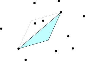
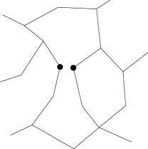
Figure 1: (a) Diamond property: one of two isosceles triangles on edge is empty. (b) Graph violating good polygon property: ratio of diagonal to boundary path is high.

Das and Joseph [5] showed that these constant dilation bounds hold for a wide variety of planar graph construction algorithms, satisfying the following two simple conditions:

• Diamond property. There is some angle $\alpha<\pi$, such that for any edge $e$ in a graph constructed by the algorithm, one of the two isosceles triangles with $e$ as a base and with apex angle $\alpha$ contains no other site. This property gets its name because the two triangles together form a diamond shape, depicted in Figure 1(a).

• Good polygon property. There is some constant $d$ such that for each face $f$ of a graph constructed by the algorithm, and any two sites $u$, $v$ that are visible to each other across the face, one of the two paths around $f$ from $u$ to $v$ has dilation at most $d$. Figure 1(b) depicts a graph violating the good polygon property.

Intuitively, if one tries to connect two vertices by a path in a graph that passes near the straight line segment between the two, there are two natural types of obstacle one encounters. The line segment one is following may cross an edge of the graph, or a face of the graph; in either case the path must go around these obstacles. The two properties above imply that neither type of detour can force the dilation of the pair of vertices to be high.

For a survey of further results on dilation, see [8]. Our interest here is in another geometric graph, the $\beta$-skeletons [12, 14], which have been of recent interest for their use in finding edges guaranteed to take part in the minimum weight triangulation [2, 10, 15] As a special case, $\beta=1$ gives the Gabriel graph, a subgraph of the Delaunay triangulation and the relative neighborhood graph, and a supergraph of the minimum spanning tree. These graphs have a definition (given below) closely related to Das and Joseph’s diamond property. The value $\beta$ is a parameter that can be taken arbitrarily close to zero; for any point set, as beta approaches zero, more and more edges are added to the $\beta$-skeleton until eventually one forms the complete graph. Therefore it seems reasonable to guess that, for sufficiently small $\beta$, the $\beta$-skeleton should have bounded dilation. Such a result would also fit well with Kirkpatrick and Radke’s motivation for introducing $\beta$-skeletons in the study of “empirical networks”: problems such as modeling the probability of the existence of a road between cities [12].

In this paper, we show that this is surprisingly not the case. For any $\beta$, we find point sets for which the $\beta$-skeleton has arbitrarily high dilation. Our construction uses fractal curves closely related to the Koch snowflake. We show that the point set can be chosen in such a way that the $\beta$-skeleton forms a path with this fractal shape; the fact that the curve has a fractal dimension greater than one then implies that the graph shortest path between its endpoints has unbounded length.

2 Beta-skeletons

The $\beta$-skeleton [12, 14] of a set of points is a graph, defined to contain exactly those edges $ab$ such that no point $c$ forms an angle $acb$ greater than $\sin^{-1}1/\beta$ (if $\beta>1$) or $\pi-\sin^{-1}\beta$ (if $\beta<1$).

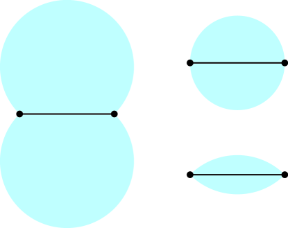
Figure 2: Empty regions for $\sqrt{2}$-skeleton, Gabriel graph, and $1/\sqrt{2}$-skeleton.

Equivalently, if $\beta>1$, the $\beta$-skeleton can be defined in terms of the union $U$ of two circles, each having $ab$ as a chord and having diameter $\beta\,d(a,b)$. Edge $ab$ is included in this graph exactly when $U$ contains no points other than $a$ and $b$.

If $\beta=1$, an edge $ab$ is included in the $\beta$-skeleton exactly when the circle having $ab$ as diameter contains no points other than $a$ and $b$. The 1-skeleton is also known as the Gabriel graph [9].

If $0<\beta<1$, there is a similar definition in terms of the intersection $I$ of two circles, each having $ab$ as a chord and having diameter $d(a,b)/\beta$. Edge $ab$ is included in the $\beta$-skeleton exactly when $I$ contains no points other than $a$ and $b$.

Figure 2 depicts these regions for $\beta=\sqrt{2}$ (union of circles), $\beta=1$ (single circle), and $\beta=1/\sqrt{2}$ (intersection of circles).

As noted above, $\beta$-skeletons were originally introduced for analyzing empirical networks. Gabriel graphs and $\beta$-skeletons have many other applications in computational morphology (combinatorial methods of representating shapes). Gabriel graphs can also be used to construct minimum spanning trees, since the gabriel graph contains the MST as a subgraph. More recently, various researchers have shown that $\beta$-skeletons (for certain values of $\beta>1$) form subgraphs of the minimum weight triangulation [2, 10, 15].

Su and Chang [13] have described a generalization of Gabriel graphs, the $k$-Gabriel graphs, in which an edge is present if its diameter circle contains at most $k-1$ other points. One can similarly generalize $\beta$-skeletons to $k$-$\beta$-skeletons. Our results can be made to hold as well for these generalizations as for the original graph classes.

3 Fractals and dilation

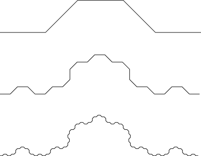
Figure 3: Fractal curves $P(\pi/4,k)$ for $k=1,2,3$.

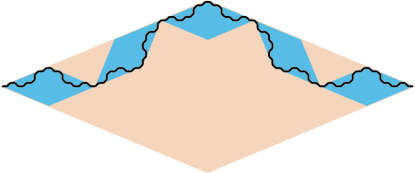
Figure 4: Fractal curve is contained in a diamond.

Our construction showing that beta-skeletons have unbounded dilation consists of a fractal curve with a recursive definition similar to that of a Koch snowflake. For a given angle $\theta$ define the polygonal path $P(\theta,1)$, by following a path of five equal-length line segments: one horizontal, one at angle $\theta$, a second horizontal, a segment at angle $-\theta$, and a third horizontal.

We then more generally define the graph $P(\theta,k)$ to be a path of $5^{k}$ line segments, formed by replacing the five segments of $P(\theta,1)$ with congruent copies of $P(\theta,k-1)$, scaled so that the two endpoints of the path are at distance one from each other. Figure 3 shows three levels of this construction. In the drawing of Figure 3, the orientations of the five copies of $P(\theta,k-1)$ alternate along the overall path, so that the horizontal copies are in the same orientation as the overall path and the other two copies are close to upside-down, but this choice of orientation is not essential to our construction.

Note that, if we denote the length of $P(\theta,k)$ by $\ell_{k}=\ell_{k}(\theta)$, then $\ell_{1}>1$ and $\ell_{k}=\ell_{1}^{k}$.

Lemma 1

$P(\theta,k)$ is contained within a diamond shape having the endpoints of the path as its diagonal, and with angle $\theta$ at those two corners of the diamond.

Proof: This follows by induction, as shown in Figure 4, since the five such diamonds containing the five copies of $P(\theta,k-1)$ fit within the larger diamond defined by the Lemma.

Lemma 2

If $\theta<(\pi-\sin^{-1}\beta)/2$, $P(\theta,k)$ is the $\beta$-skeleton of its vertices.

Proof: We show that, if $a$ and $b$ are non-adjacent vertices in the path, then there is some $c$ forming an angle of at least $\pi-\sin^{-1}\beta$. We can assume that $a$ and $b$ are in different copies of $P(\theta,k-1)$, since otherwise the result would hold by induction. But no matter where one places two points in different copies of the small diamonds containing the copies of $P(\theta,k-1)$ (depicted in Figure 4), we can choose one of the three interior vertices of $P(\theta,1)$ as the third point $c$ forming an angle $acb\geq\pi-2\theta$. The result follows from the assumed inequality relating $\theta$ to $\beta$.

For instance, the graphs $P(\pi/4,k)$ depicted in Figure 3 are Gabriel graphs of their vertices. A more careful analysis shows that larger values of $\theta$ still result in a $\beta$-skeleton: if the orientations of the copies of $P(\theta,k-1)$ that form $P(\theta,k)$ are chosen carefully, $P(\theta,k)$ is contained in only half the diamond of Lemma 1, and angle $acb$ in the proof above can be shown to be $\geq\pi-3\theta/2$.

Theorem 1

For any $\beta>0$ there is a $c>0$ such that $\beta$-skeletons of $n$-point sets have dilation $\Omega(n^{c})$.

Proof: We have seen that we can choose a $\theta$ such that the graphs $P(\theta,k)$ are $\beta$-skeletons. Since the endpoints of the path are at distance one from each other, the dilation of $P(\theta,k)$ is $\ell_{k}=\ell_{1}^{k}$. Each such graph has $n=5^{k}+1$ vertices and dilation $\ell_{1}^{k}=n^{\mathop{\rm log}_{5}\ell_{1}-o(1)}$. Since $\ell_{1}>1$, $\mathop{\rm log}_{5}\ell_{1}>0$.

4 Upper Bounds

We have shown a lower bound of $\Omega(n^{c})$ for the dilation of $\beta$-skeletons, where $c$ is a constant depending on $\beta$, and approaching zero as $\beta$ approaches zero. This behavior of having length a fractional power of $n$ is characteristic of fractal curves; is it inherent in $\beta$-skeletons or an artifact of our fractal construction? We now show the former by proving an upper bound on dilation of the same form.

To do this, we define an algorithm for finding short paths in $\beta$-skeletons. As a first start towards such an algorithm, we use the following simple recursion: to find a path from $s$ to $t$, test whether edge $st$ exists in the $\beta$-skeleton. If so, use that edge as path. If not, some $r$ forms a large angle $srt$; concatenate the results of recursively finding paths from $s$ to $r$ and $r$ to $t$.

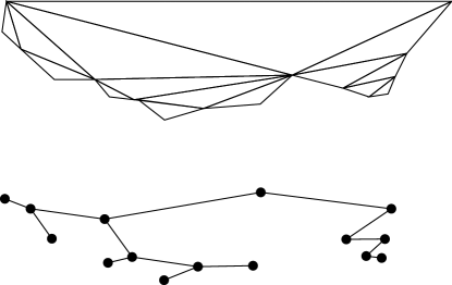
Figure 5: Tree of triangles and corresponding abstract tree.

For $\beta\leq 1$, $sr$ and $rt$ are shorter than $st$, so this algorithm always terminates; we assume throughout the rest of the section that $\beta\leq 1$. We can represent the path it finds as a tree of triangles, all having an angle of at least $\pi-\sin^{-1}\beta$, rooted at triangle $srt$ (Figure 5). The hypotenuse of each triangle in this tree is equal to one of the two shorter sides of its parent. Note that the triangles may overlap geometrically, or even coincide; we avoid complications arising from this possibility by only using the figure’s combinatorial tree structure. We will bound the length of the path found by this algorithm by manipulating trees of this form. For any similarly defined tree of triangles, we define the boundary length of the tree to be the following formula:

$$|T|={\rm dist}(s,t)+\sum_{\Delta\in T}({\rm perim}(\Delta)-2\cdot{\rm hypotenuse}(\Delta)).$$

In other words, we sum the lengths of all the short sides of the triangles, and subtract the lengths of all non-root hypotenuses. If the tree forms a non-self-intersecting polygon, such as the one shown in the figure, this is distance from $s$ to $t$ “the long way” around the polygon’s perimeter

Lemma 3

For the tree defined by the algorithm above, $|T|$ is the length of the path constructed by the algorithm.

Proof: This can be shown by induction using the fact that the path from $s$ to $t$ is formed by concatenating the paths from $s$ to $r$ and $r$ to $t$.

Our bound will depend on the number of leaves in the tree produced above. However, this number may be very large, larger than $n$, because the same vertex of our input point set may be involved in triangles in many unrelated parts of the tree. Our first step is to prune the tree to produce one that still corresponds in a sense to a path in the $\beta$-skeleton, but with a good bound on the number of leaves.

Lemma 4

For any $\beta\leq 1$, we can find a tree like the one described above, with at most $2n$ leaves, for which $|T|$ is the length of some path in the $\beta$-skeleton from $s$ to $t$.

Proof: Define a “leaf vertex” to be the vertex opposite the hypotenuse of a leaf triangle in $T$. We prune the tree one step at a time until each vertex appears at most twice as a leaf vertex. At each step, the path corresponding to $T$ (and with length at most $|T|$) will visit all the leaf vertices in tree order (as well as possibly visiting some other vertices coming from interior nodes of the tree).

Suppose some vertex $v$ appears three or more times. Then we prune $T$ by removing all subtrees descending from the path between the first and last appearance of $v$ (occurring between the two appearences in tree order), and we shorten the corresponding path by removing the portion of it between these two appearances of $v$. At each step, the change to $|T|$ comes from subtracting some triangle short side lengths corresponding to the subtrees removed from $T$, as well as adding some hypotenuses of triangles from the same subtrees. Each subtracted side length that is not cancelled by an added hypotenuse corresponds to one of the edges removed from the path, so the total reduction in $|T|$ is at most as great as the total reduction in the length of the path, and the invariant that $|T|$ bounds the path length is maintained. After this pruning, there will be no leaves between the two appearances of $v$, and no new leaves are created elsewhere in the tree, so the invariant that the path visits the leaf vertices in order is also maintained.

This pruning process removes at least one appearance of $v$, and so can be repeated at most finitely many times before terminating.

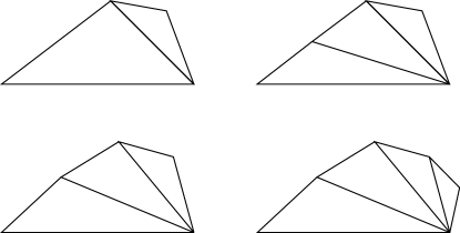
Figure 6: Making single-leaf tree longer: subdivide triangles, increase angles, add children.

We use induction on the number of leaves to prove bounds on $|T|$. The following lemma forms the base case:

Lemma 5

Let $T$ be a tree of triangles, all having an angle of at least $\theta>\pi/2$ opposite the edge connecting to the parent in the tree, with exactly one leaf triangle, and scaled so that the hypotenuse of the root triangle has length $1$. Then $|T|\leq-1/\cos\theta$.

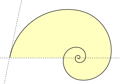
Figure 7: Logarithmic spiral formed by keeping fixed angle to destination point.

Proof: Since $|T|$ does not depend on the ordering of tree nodes, we can assume without loss of generality that each node’s child is on the left. For any such tree, we can increase $|T|$ by performing a sequence of the following steps: (1) If any triangle has an angle greater than $\theta$, change it to one having an angle exactly equal to $\theta$, without changing any other triangle shapes. (2) If any triangle has a ratio of left to right side lengths less than some value $C$, split it into two triangles by adding a vertex on the right side. (3) Add a child to the leaf of $T$. These steps are depicted in Figure 6.

The result of this sequence of transformations is the concatenation of many triangles with angles equal to $\theta$, very short left sides, and right sides with length close to that of the hypotenuse. In the limit we get a curve from $s$ to $t$ formed by moving in a direction forming an angle $\pi-\theta$ to $t$, namely the logarithmic spiral (Figure 7). Integrating the distance traveled on this spiral against the amount by which the distance to $t$ is reduced shows that it has the length formula claimed in the lemma. Since we reach this limit by a monotonically increasing sequence of tree lengths, starting with any finite one-leaf tree, any finite tree must have length less than this limit.

More generally, we have the following result.

Lemma 6

Let $T$ be a tree of triangles, all having an angle of at least $\theta>\pi/2$ opposite the edge connecting to the parent in the tree, with $k$ leaf triangles, and scaled so that the hypotenuse of the root triangle has length $1$. Then $|T|\leq(-1/\cos\theta)^{1+\lfloor\mathop{\rm log}_{2}k\rfloor}$.

Proof: We prove the result by induction on $k$; Lemma 5 forms the base case. If there is more than one leaf in $T$, form a smaller tree $T^{\prime}$ by removing from $T$ each path from a leaf to the nearest ancestor with more than one child. These paths are disjoint, and each such removal replaces a subtree with one leaf by the edge at the root of the subtree, so using Lemma 5 again shows that $|T|\leq-|T^{\prime}|/\cos\theta$. Each leaf in $T^{\prime}$ has two leaf descendants in $T$, so the number of leaves in $T$ is at most $k/2$ and the result follows.

This, finally, provides a bound on $\beta$-skeleton dilation.

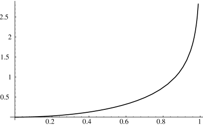
Figure 8: Exponent in the bound of Theorem 2, as a function of $\beta$.

Theorem 2

For $\beta<\sqrt{3}/2\approx 0.866025$, any $\beta$-skeleton has dilation $O(n^{c})$, where $c<1$ is a constant depending on $\beta$ and going to zero in the limit as $\beta$ goes to zero.

Proof: We have seen (Lemma 4) that we can connect any pair of vertices in the skeleton by a path with length bounded by $|T|$, where $T$ is a tree of triangles in which all angles are at least $\pi-\sin^{-1}\beta$, and where $T$ has at most $2n$ leaves. By Lemma 6, the length of such a tree is at most

$$(-1/\cos(\pi-\sin^{-1}\beta))^{1+\lfloor\mathop{\rm log}_{2}2n\rfloor}=O\big{(}n^{\mathop{\rm log}_{2}{{\scriptstyle-1}\over{\scriptstyle\cos(\pi-\sin^{-1}\beta)}}}\big{)}=O\big{(}n^{-{1\over 2}\mathop{\rm log}_{2}(1-\beta^{2})}\big{)}$$

which has the form specified in the statement of the theorem.

Figure 8 shows the growth of the exponent $c$ as a function of $\beta$. For $\sqrt{3}/2\leq\beta\leq 1$, the theorem does not give the best bounds; a bound of $n-1$ on dilation can be proven using the fact that the skeleton contains the minimum spanning tree.

References

- [1]
- [2] S. Cheng and Y. Xu. Approaching the largest -skeleton within the minimum weight triangulation, manuscript cited by [6], 1995.
- [3] L. P. Chew. There is a planar graph almost as good as the complete graph. Proc. 2nd ACM Symp. Comp. Geom., 1986, pp. 169–177.
- [4] L. P. Chew. There are planar graphs almost as good as the complete graph. J. Comp. Sys. Sci., vol. 39, 1989, pp. 205–219.
- [5] G. Das and D. Joseph. Which triangulations approximate the complete graph? Proc. Int. Symp. Optimal Algorithms. Springer LNCS 401, 1989, pp. 168–192.
- [6] M. Dickerson and M. Montague. A (usually) connected subgraph of the minimum weight triangulation. Proc. 5th MSI-Stony Brook Worksh. Comp. Geom., 1995.
- [7] D. P. Dobkin, S. J. Friedman, and K. J. Supowit. Delaunay graphs are almost as good as complete graphs. Disc. Comp. Geom., vol. 5, 1990, pp. 399–407.
- [8] D. Eppstein. Spanning trees and spanners. Tech. Report 96-16, Dept. Information and Computer Science, University of California, Irvine, 1996.
- [9] K. R. Gabriel and R. R. Sokal. A new statistical approach to geographic variation analysis. Systematic Zoology, vol. 18, 1969, pp. 259–278.
- [10] J. M. Keil. Computing a subgraph of the minimum weight triangulation. Comp. Geom. Theory & Appl., vol. 4, 1994, pp. 13–26.
- [11] J. M. Keil and C. A. Gutwin. The Delaunay triangulation closely approximates the complete Euclidean graph. Proc. 1st Worksh. Algorithms and Data Structures. Springer LNCS 382, 1989, pp. 47–56.
- [12] D. G. Kirkpatrick and J. D. Radke. A framework for computational morphology. Computational Geometry, North-Holland, 1985, pp. 217–248.
- [13] T.-H. Su and R.-C. Chang. The -Gabriel graphs and their applications. Int. Symp. Algorithms, Springer LNCS 450, 1990, pp. 66–75.
- [14] R. C. Veltkamp. The gamma-neighborhood graph. Comp. Geom. Theory & Appl., vol. 1, 1992, pp. 227–246.
- [15] B.-T. Yang. A better subgraph of the minimum weight triangulation. Inf. Proc. Lett., vol. 56, 1995, pp. 255–258.