Events in Property Patterns

Abstract

A pattern-based approach to the presentation, codification and reuse of property specifications for finite-state verification was proposed by Dwyer and his colleagues in [4, 3]. The patterns enable non-experts to read and write formal specifications for realistic systems and facilitate easy conversion of specifications between formalisms, such as LTL, CTL, QRE. In this paper we extend the pattern system with events — changes of values of variables in the context of LTL.

1 Introduction

Temporal logics (TL) (e.g., [1], [5], [9], [16], [12]) have received a lot of attention in the research community. Not only are they useful for specifying properties of systems, recent advances in model-checking allow effective automatic checking of models of systems against such properties, e.g. using tools like SPIN [8] and SMV [13].

One important obstacle to using temporal logic is the ability to express complex properties correctly. To remedy this problem, Dwyer and his colleagues have proposed a pattern-based approach to the presentation, codification and reuse of property specifications. The system allows patterns like “$P$ is absent between $Q$ and $S$” or “$S$ precedes $P$ between $Q$ and $R$” to be easily expressed in and translated between linear-time temporal logic (LTL) [11], computational tree logic (CTL) [2], quantified regular expressions (QRE) [15], and other state-based and event-based formalisms. Dwyer et. al. also performed a large-scale study in which specifications containing over 500 temporal properties were collected and analyzed. They noticed that over 90% of these could be classified under one of the proposed patterns [4].

In earlier work [20], we used the Promela/SPIN framework to model the Production Cell system. We attempted to use the pattern-base approach to help us formalize properties of this system in LTL. However, we found that the approach could not be applied directly, because our properties used events — changes of values of variables, e.g., “magnet should become deactivated”, which we wanted to formalize as “magnet is active now and will be inactive in the next state”. We called such events edges.

LTL is a temporal logic comprised of propositional formulas and temporal connectives $\mathord{\Box}$ (“always”), $\mathord{\Diamond}$ (“eventually”), $\mathord{\circ}$ (“next”), and $\mathbin{\mathcal{U}}$ (“until”). The first three operators are unary, while the last one is binary. $\mathbin{\mathcal{U}}$ is the strong until; that is, it requires that $B$ actually happen sometime in the future. In this context, we define edges as follows:

$$\begin{array}[]{rcl>{$}c<{$}>{$}l<{$}}\mathord{\uparrow}A&\mathbin{\mbox{\large$\boldsymbol{=}$}}&\lnot A\land\mathord{\circ}A&---&up or rising edge\\ \mathord{\downarrow}A&\mathbin{\mbox{\large$\boldsymbol{=}$}}&A\land\mathord{\circ}\lnot A&---&down or falling edge\\ \mathord{\updownarrow}A&\mathbin{\mbox{\large$\boldsymbol{=}$}}&\mathord{\uparrow}A\lor\mathord{\downarrow}A&---&any edge\end{array}$$

LTL formulas containing events may have problems caused by the use of the “next” operator in the definition of edges. Temporal formulas that make use of “next” may not be closed under stuttering, i.e. their interpretation may be modified by transitions that leave the system in the same state (“stutter”). As we discuss later in the paper, this is an essential property for effective use of temporal formulas.

Model-checking allows relatively novice users to verify correctness of their systems quickly and effectively. However, it is essential that these users are able to specify correctness criteria in the appropriate temporal logic. For example, effective use of SPIN [8] depends critically on being able to express such criteria in LTL. Under the presence of events, it is often quite complex (see  [19] for a thorough discussion). In this paper we extend the properties of Dwyer et. al. to include events in LTL properties. The rest of the paper is organized as follows: Section 2 overviews the pattern-based system. Section 3 presents our extension to the pattern-based system and discusses the extension process. Section 4 contains an informal summary of our treatment of closure under stuttering and presents a set of theorems that allow syntactic checking of formulas for this property. In addition, it shows how to use these theorems to prove that our extensions of the pattern-based system are closed under stuttering. Section 5 concludes the paper.

2 Overview of the Pattern-Based Approach

Figure 1: A Pattern Hierarchy.

In this section we survey the pattern-based approach. For more information, please refer to [3, 4]. The patterns are organized hierarchically based on their semantics, as illustrated in Figure 1. Some of the patterns are described below:

Absence	A condition does not occur within a scope;
Existence	A condition must occur within a scope;
Universality	A condition occurs throughout a scope;
Response	A condition must always be followed by another within a scope;
Precedence	A condition must always be preceded by another within a scope.

Each pattern is associated with several scopes — the regions of interest over which the condition is evaluated. There are five basic kinds of scopes:

A.	Global	The entire state sequence;
B.	Before $R$	The state sequence up to condition $R$;
C.	After $Q$	The state sequence after condition $Q$;
D.	Between $Q$ and $R$	The part of the state sequence between condition $Q$ and
	condition $R$;
E.	After $Q$ Until $R$	Similar to the previous one, except that the designated
	part of the state sequence continues even if the second condition does not
	occur.

These scopes are depicted in Figure 2. The scopes were initially defined in [4] to be closed-left, open-right intervals, although it is also possible to define other combinations, such as open-left, closed-right intervals.

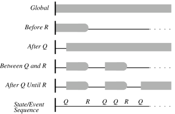
Figure 2: Pattern Scopes.

For example, an LTL formulation of the property “$S$ precedes $P$ between $Q$ and $R$” (Precedence pattern with “between $Q$ and $R$” scope) is:

$$\mathord{\Box}((Q\land\mathord{\Diamond}R)\Rightarrow(\lnot P\mathbin{\mathcal{U}}(S\lor R)))$$

Even though the pattern system is formalism-independent [3], in this paper we are only concerned with the expression of properties in LTL.

S

3 Edges and the Pattern-Based System

LTL is a state-based formalism, and thus the original pattern system does not specify the expression of events in LTL. In this section we show how to include reasoning about events to the pattern system. These events can be used for specifying conditions as well as for defining the bounding scopes.

We start by introducing some notation that allows us a more compact representation of properties. We define the weak version of “until” as:

$$A\mathbin{\mathcal{W}}B=\mathord{\Box}A\lor(A\mathbin{\mathcal{U}}B)$$

That is, we no longer require $B$ to happen in the future; if it does not, than $A$ should hold indefinitely. Another useful operator is “precedes”:

$$A\mathbin{\mathcal{P}}B=\lnot(\lnot A\mathbin{\mathcal{U}}B)$$

That is, we want $A$ to hold before $B$ does. Note that in this case $B$ may never happen. Also, we use $\mathord{y\lhd x\rhd z}$ to indicate $\mathord{\mathbf{if}\;x\;\mathbf{then}\;y\;\mathbf{else}\;z}$, or $(x\land y)\lor(\lnot x\land z)$. Finally, we write $\top$ and $\bot$ to indicate boolean values true and false, respectively.

Since our extension involves edges, we give a few relevant properties below:

$$\mathord{\Box}\mathord{\uparrow}A = \bot$$ (1)

$$\mathord{\Box}\mathord{\downarrow}A = \bot$$ (2)

$$\mathord{\uparrow}A\mathbin{\mathcal{U}}B = B\lor(\mathord{\uparrow}A\land\mathord{\circ}B)$$ (3)

Properties (1) and (2) indicate that edges of the same type cannot occur in every state of the system, whereas property (3) allows us to replace an “until” with a propositional expression.

We have explored the concept of edges in [19, 18], and list some of edge properties in the Appendix.

3.1 Extending the Pattern System

Introducing edges into the patterns generates an explosion in the number of formulas: conditions can be state-based or edge-based, inclusive or exclusive, and the interval ends can be either opened or closed. Our extension does not include all the possibilities, but rather a significant and representative set of them, as discussed below.

We were able to extend five of the nine patterns: Absence (Figure 3), Existence (Figure 4), Universality (Figure 5), Response (Figure 7), Precedence (Figure 6). For each of the five scopes, we list four formulas corresponding to the four combinations of state-based and edge-based conditions and interval bounds we have considered:

0.	$P$, $S$ — states,	$Q$, $R$ — states;
1.	$P$, $S$ — states,	$Q$, $R$ — up edges;
2.	$P$, $S$ — up edges,	$Q$, $R$ — states;
3.	$P$, $S$ — up edges,	$Q$, $R$ — up edges.

Combination 0 corresponds to the original formulation of [3], where all of $P$, $S$, $Q$ and $R$ are state-based. The remaining three combinations are our extensions to the pattern system. We assume that multiple events can happen simultaneously, but only consider closed-left, open-right intervals, as in the original system. Also, we consider events $P$ and $S$ to be exclusive in the Precedence pattern and inclusive in the Response pattern. We note, however, that it is perfectly possible to have formulas for all other combinations of interval bounds. Down edges can be substituted for up edges without changing the formulas. We have modified several of the 0-formulas (i.e. state-based conditions and intervals) from their original formulations of [3] to remove assumptions of interleaving and make them consistent with the closed-left, open-right intervals. Note that in the case of the Universality pattern, we do not list formulas for edge-based events as edges cannot be universally present (by (1) and (2)).

$\begin{array}[]{rl}\lx@intercol\hfil$A. Globally$\hfil\lx@intercol\\ 0.&\mathord{\Box}\lnot P\\ 1.&\mathord{\Box}\lnot P\\ 2.&\mathord{\Box}\lnot\mathord{\uparrow}P\\ 3.&\mathord{\Box}\lnot\mathord{\uparrow}P\end{array}$ $\begin{array}[]{rl}\lx@intercol\hfil$B. Before $R$$\hfil\lx@intercol\\ 0.&\mathord{\Diamond}R\Rightarrow(\lnot P\mathbin{\mathcal{U}}R)\\ 1.&\mathord{\Diamond}\mathord{\uparrow}R\Rightarrow(\mathord{\uparrow}R\mathbin{\mathcal{P}}P)\\ 2.&\mathord{\Diamond}R\Rightarrow(\lnot\mathord{\uparrow}P\mathbin{\mathcal{U}}R)\\ 3.&\mathord{\Diamond}\mathord{\uparrow}R\Rightarrow(\lnot\mathord{\uparrow}P\mathbin{\mathcal{U}}\mathord{\uparrow}R)\end{array}$ $\begin{array}[]{rl}\lx@intercol\hfil$C. After $Q$$\hfil\lx@intercol\\ 0.&\mathord{\Box}(Q\Rightarrow\mathord{\Box}\lnot P)\\ 1.&\mathord{\Box}(\mathord{\uparrow}Q\Rightarrow\mathord{\circ}\mathord{\Box}\lnot P)\\ 2.&\mathord{\Box}(Q\Rightarrow\mathord{\Box}\lnot\mathord{\uparrow}P)\\ 3.&\mathord{\Box}(\mathord{\uparrow}Q\Rightarrow\mathord{\Box}\lnot\mathord{\uparrow}P)\end{array}$ $\begin{array}[]{rl}\lx@intercol\hfil$D. Between $Q$ and $R$$\hfil\lx@intercol\\ 0.&\mathord{\Box}((Q\land\mathord{\Diamond}R)\Rightarrow(\lnot P\mathbin{\mathcal{U}}R))\\ 1.&\mathord{\Box}((\mathord{\uparrow}Q\land\mathord{\Diamond}\mathord{\uparrow}R\land\lnot\mathord{\uparrow}R)\Rightarrow\mathord{\circ}(\mathord{\uparrow}R\mathbin{\mathcal{P}}P))\\ 2.&\mathord{\Box}((Q\land\mathord{\Diamond}R)\Rightarrow(\lnot\mathord{\uparrow}P\mathbin{\mathcal{U}}R))\\ 3.&\mathord{\Box}((\mathord{\uparrow}Q\land\mathord{\Diamond}\mathord{\uparrow}R)\Rightarrow(\lnot\mathord{\uparrow}P\mathbin{\mathcal{U}}\mathord{\uparrow}R))\end{array}$ $\begin{array}[]{rl}\lx@intercol\hfil$E. After $Q$ Until $R$$\hfil\lx@intercol\\ 0.&\mathord{\Box}((Q\land\mathord{\Diamond}P)\Rightarrow(\lnot P\mathbin{\mathcal{U}}R))\\ 1.&\mathord{\Box}((\mathord{\uparrow}Q\land\lnot\mathord{\uparrow}R\land\mathord{\circ}\mathord{\Diamond}P)\Rightarrow\mathord{\circ}(\mathord{\uparrow}R\mathbin{\mathcal{P}}P))\\ 2.&\mathord{\Box}(Q\Rightarrow(\lnot\mathord{\uparrow}P\mathbin{\mathcal{W}}R))\\ 3.&\mathord{\Box}(\mathord{\uparrow}Q\Rightarrow(\lnot\mathord{\uparrow}P\mathbin{\mathcal{W}}\mathord{\uparrow}R))\end{array}$

Figure 3: Formulations of the Absence Pattern

$\begin{array}[]{rl}\lx@intercol\hfil$A. Globally$\hfil\lx@intercol\\ 0.&\mathord{\Diamond}P\\ 1.&\mathord{\Diamond}P\\ 2.&\mathord{\Diamond}\mathord{\uparrow}P\\ 3.&\mathord{\Diamond}\mathord{\uparrow}P\end{array}$ $\begin{array}[]{rl}\lx@intercol\hfil$B. Before $R$$\hfil\lx@intercol\\ 0.&\mathord{\Diamond}R\Rightarrow(P\mathbin{\mathcal{P}}R)\\ 1.&\mathord{\Diamond}\mathord{\uparrow}R\Rightarrow(\lnot\mathord{\uparrow}R\mathbin{\mathcal{U}}P)\\ 2.&\mathord{\Diamond}R\Rightarrow(\mathord{\uparrow}P\mathbin{\mathcal{P}}R)\\ 3.&\mathord{\Diamond}\mathord{\uparrow}R\Rightarrow(\mathord{\uparrow}P\mathbin{\mathcal{P}}\mathord{\uparrow}R)\end{array}$ $\begin{array}[]{rl}\lx@intercol\hfil$C. After $Q$$\hfil\lx@intercol\\ 0.&\mathord{\Diamond}Q\Rightarrow\mathord{\Diamond}(Q\land\mathord{\Diamond}P)\\ 1.&\mathord{\Diamond}\mathord{\uparrow}Q\Rightarrow\mathord{\Diamond}(\mathord{\uparrow}Q\land\mathord{\circ}\mathord{\Diamond}P)\\ 2.&\mathord{\Diamond}Q\Rightarrow\mathord{\Diamond}(Q\land\mathord{\Diamond}\mathord{\uparrow}P)\\ 3.&\mathord{\Diamond}\mathord{\uparrow}Q\Rightarrow\mathord{\Diamond}(\mathord{\uparrow}Q\land\mathord{\Diamond}\mathord{\uparrow}P)\end{array}$ $\begin{array}[]{rl}\lx@intercol\hfil$D. Between $Q$ and $R$$\hfil\lx@intercol\\ 0.&\mathord{\Box}((Q\land\mathord{\Diamond}R)\Rightarrow((P\mathbin{\mathcal{P}}R)\land\lnot R))\\ 1.&\mathord{\Box}((\mathord{\uparrow}Q\land\mathord{\Diamond}\mathord{\uparrow}R)\Rightarrow(\mathord{\circ}(\lnot\mathord{\uparrow}R\mathbin{\mathcal{U}}P)\land\lnot\mathord{\uparrow}R))\\ 2.&\mathord{\Box}((Q\land\mathord{\Diamond}R)\Rightarrow((\mathord{\uparrow}P\mathbin{\mathcal{P}}R)\land\lnot R))\\ 3.&\mathord{\Box}((\mathord{\uparrow}Q\land\mathord{\Diamond}\mathord{\uparrow}R)\Rightarrow((\mathord{\uparrow}P\mathbin{\mathcal{P}}\mathord{\uparrow}R)\land\lnot\mathord{\uparrow}R))\end{array}$ $\begin{array}[]{rl}\lx@intercol\hfil$E. After $Q$ Until $R$$\hfil\lx@intercol\\ 0.&\mathord{\Box}(Q\Rightarrow\mathord{(P\mathbin{\mathcal{P}}R)\land\lnot R\lhd\mathord{\Diamond}R\rhd\mathord{\Diamond}P})\\ 1.&\mathord{\Box}(\mathord{\uparrow}Q\Rightarrow\mathord{\circ}(\lnot\mathord{\uparrow}R\mathbin{\mathcal{U}}P)\land\lnot\mathord{\uparrow}R)\\ 2.&\mathord{\Box}(Q\Rightarrow\mathord{(\mathord{\uparrow}P\mathbin{\mathcal{P}}R)\land\lnot R\lhd\mathord{\Diamond}R\rhd\mathord{\Diamond}\mathord{\uparrow}P})\\ 3.&\mathord{\Box}(\mathord{\uparrow}Q\Rightarrow\mathord{(\mathord{\uparrow}P\mathbin{\mathcal{P}}\mathord{\uparrow}R)\land\lnot\mathord{\uparrow}R\lhd\mathord{\Diamond}\mathord{\uparrow}R\rhd\mathord{\Diamond}\mathord{\uparrow}P})\end{array}$

Figure 4: Formulations of the Existence Pattern

$\begin{array}[]{rl}\lx@intercol\hfil$A. Globally$\hfil\lx@intercol\\ 0.&\mathord{\Box}P\\ 1.&\mathord{\Box}P\end{array}$ $\begin{array}[]{rl}\lx@intercol\hfil$B. Before $R$$\hfil\lx@intercol\\ 0.&\mathord{\Diamond}R\Rightarrow(P\mathbin{\mathcal{U}}R)\\ 1.&\mathord{\Diamond}\mathord{\uparrow}R\Rightarrow(\mathord{\uparrow}R\mathbin{\mathcal{P}}\lnot P)\end{array}$ $\begin{array}[]{rl}\lx@intercol\hfil$C. After $Q$$\hfil\lx@intercol\\ 0.&\mathord{\Box}(Q\Rightarrow\mathord{\Box}P)\\ 1.&\mathord{\Box}(\mathord{\uparrow}Q\Rightarrow\mathord{\circ}\mathord{\Box}P)\end{array}$ $\begin{array}[]{rl}\lx@intercol\hfil$D. Between $Q$ and $R$$\hfil\lx@intercol\\ 0.&\mathord{\Box}((Q\land\mathord{\Diamond}R)\Rightarrow(P\mathbin{\mathcal{U}}R))\\ 1.&\mathord{\Box}((\mathord{\uparrow}Q\land\mathord{\Diamond}\mathord{\uparrow}R\land\lnot\mathord{\uparrow}R)\Rightarrow\mathord{\circ}(\mathord{\uparrow}R\mathbin{\mathcal{P}}\lnot P))\end{array}$ $\begin{array}[]{rl}\lx@intercol\hfil$E. After $Q$ Until $R$$\hfil\lx@intercol\\ 0.&\mathord{\Box}(Q\Rightarrow P\mathbin{\mathcal{W}}R)\\ 1.&\mathord{\Box}(\mathord{\uparrow}Q\Rightarrow\mathord{\circ}\mathord{(\mathord{\uparrow}R\mathbin{\mathcal{P}}\lnot P)\lhd\mathord{\Diamond}\mathord{\uparrow}R\rhd\mathord{\Box}P})\end{array}$

Figure 5: Formulations of the Universality Pattern

$\begin{array}[]{rl}\lx@intercol\hfil$A. Globally$\hfil\lx@intercol\\ 0.&\mathord{\Diamond}P\Rightarrow S\mathbin{\mathcal{P}}P\\ 1.&\mathord{\Diamond}P\Rightarrow S\mathbin{\mathcal{P}}P\\ 2.&\mathord{\Diamond}\mathord{\uparrow}P\Rightarrow\mathord{\uparrow}S\mathbin{\mathcal{P}}\mathord{\uparrow}P\\ 3.&\mathord{\Diamond}\mathord{\uparrow}P\Rightarrow\mathord{\uparrow}S\mathbin{\mathcal{P}}\mathord{\uparrow}P\end{array}$ $\begin{array}[]{rl}\lx@intercol\hfil$E. After $Q$ Until $R$$\hfil\lx@intercol\\ 0.&\mathord{\Box}(Q\Rightarrow(\mathord{\Diamond}P\Rightarrow\lnot P\mathbin{\mathcal{U}}((S\land\lnot P)\lor R)))\\ 1.&\mathord{\Box}(\mathord{\uparrow}Q\Rightarrow\mathord{\circ}(\mathord{\Diamond}P\Rightarrow((\lnot\mathord{\uparrow}R\mathbin{\mathcal{U}}P)\Rightarrow(S\mathbin{\mathcal{P}}P))))\\ 2.&\mathord{\Box}(Q\Rightarrow(\mathord{\Diamond}P\Rightarrow\lnot\mathord{\uparrow}P\mathbin{\mathcal{U}}((\mathord{\uparrow}S\land\lnot\mathord{\uparrow}P)\lor R)))\\ 3.&\mathord{\Box}(\mathord{\uparrow}Q\Rightarrow\mathord{\circ}(\mathord{\Diamond}P\Rightarrow((\mathord{\uparrow}P\mathbin{\mathcal{P}}\mathord{\uparrow}R)\Rightarrow(\mathord{\uparrow}S\mathbin{\mathcal{P}}\mathord{\uparrow}P))))\end{array}$ $\begin{array}[]{rl}\lx@intercol\hfil$B. Before $R$$\hfil\lx@intercol\\ 0.&\mathord{\Diamond}R\Rightarrow(\lnot P\mathbin{\mathcal{U}}((S\land\lnot P)\lor R))\\ 1.&\mathord{\Diamond}\mathord{\uparrow}R\Rightarrow((\lnot\mathord{\uparrow}R\mathbin{\mathcal{U}}P)\Rightarrow(S\mathbin{\mathcal{P}}P))\\ 2.&\mathord{\Diamond}R\Rightarrow\lnot\mathord{\uparrow}P\mathbin{\mathcal{U}}((\mathord{\uparrow}S\land\lnot\mathord{\uparrow}P)\lor R)\\ 3.&\mathord{\Diamond}\mathord{\uparrow}R\Rightarrow((\mathord{\uparrow}P\mathbin{\mathcal{P}}\mathord{\uparrow}R)\Rightarrow(\mathord{\uparrow}S\mathbin{\mathcal{P}}\mathord{\uparrow}P))\end{array}$ $\begin{array}[]{rl}\lx@intercol\hfil$C. After $Q$$\hfil\lx@intercol\\ 0.&\mathord{\Diamond}Q\Rightarrow\mathord{\Diamond}(Q\land(\mathord{\Diamond}P\Rightarrow(S\mathbin{\mathcal{P}}P)))\\ 1.&\mathord{\Diamond}\mathord{\uparrow}Q\Rightarrow\mathord{\Diamond}(\mathord{\uparrow}Q\land\mathord{\circ}(\mathord{\Diamond}P\Rightarrow(S\mathbin{\mathcal{P}}P)))\\ 2.&\mathord{\Diamond}Q\Rightarrow\mathord{\Diamond}(Q\land(\mathord{\Diamond}\mathord{\uparrow}P\Rightarrow(\mathord{\uparrow}S\mathbin{\mathcal{P}}\mathord{\uparrow}P)))\\ 3.&\mathord{\Diamond}\mathord{\uparrow}Q\Rightarrow\mathord{\Diamond}(\mathord{\uparrow}Q\land(\mathord{\Diamond}\mathord{\uparrow}P\Rightarrow(\mathord{\uparrow}S\mathbin{\mathcal{P}}\mathord{\uparrow}P)))\end{array}$ $\begin{array}[]{rl}\lx@intercol\hfil$D. Between $Q$ and $R$$\hfil\lx@intercol\\ 0.&\mathord{\Box}((Q\land\mathord{\Diamond}R)\Rightarrow(\lnot P\mathbin{\mathcal{U}}((S\land\lnot P)\lor R)))\\ 1.&\mathord{\Box}((\mathord{\uparrow}Q\land\lnot\mathord{\uparrow}R\mathord{\circ}\mathord{\Diamond}\mathord{\uparrow}R)\Rightarrow\mathord{\circ}((\lnot\mathord{\uparrow}R\mathbin{\mathcal{U}}P)\Rightarrow(S\mathbin{\mathcal{P}}P)))\\ 2.&\mathord{\Box}((Q\land\mathord{\Diamond}R)\Rightarrow(\lnot\mathord{\uparrow}P\mathbin{\mathcal{U}}((\mathord{\uparrow}S\land\lnot\mathord{\uparrow}P)\lor R)))\\ 3.&\mathord{\Box}((\mathord{\uparrow}Q\land\lnot\mathord{\uparrow}R\mathord{\circ}\mathord{\Diamond}\mathord{\uparrow}R)\Rightarrow\mathord{\circ}((\mathord{\uparrow}P\mathbin{\mathcal{P}}\mathord{\uparrow}R)\Rightarrow(\mathord{\uparrow}S\mathbin{\mathcal{P}}\mathord{\uparrow}P)))\end{array}$ $\begin{array}[]{l}\rule{0.0pt}{2.84526pt}\end{array}$

Figure 6: Formulations of the Precedence Pattern

$\begin{array}[]{rl}\lx@intercol\hfil$A. Globally$\hfil\lx@intercol\\ 0.&\mathord{\Box}(P\Rightarrow\mathord{\Diamond}S)\\ 1.&\mathord{\Box}(P\Rightarrow\mathord{\Diamond}S)\\ 2.&\mathord{\Box}(\mathord{\uparrow}P\Rightarrow\mathord{\Diamond}\mathord{\uparrow}S)\\ 3.&\mathord{\Box}(\mathord{\uparrow}P\Rightarrow\mathord{\Diamond}\mathord{\uparrow}S)\end{array}$ $\begin{array}[]{rl}\lx@intercol\hfil$B. Before $R$$\hfil\lx@intercol\\ 0.&\mathord{\Diamond}R\Rightarrow(P\Rightarrow(\lnot R\mathbin{\mathcal{U}}S))\mathbin{\mathcal{U}}R\\ 1.&\mathord{\Diamond}\mathord{\uparrow}R\Rightarrow((P\Rightarrow(\lnot\mathord{\uparrow}R\mathbin{\mathcal{U}}S))\land\lnot\mathord{\uparrow}R)\mathbin{\mathcal{U}}(\mathord{\uparrow}R\land(P\Rightarrow Q))\\ 2.&\mathord{\Diamond}R\Rightarrow(\mathord{\uparrow}P\Rightarrow(\lnot R\mathbin{\mathcal{U}}\mathord{\uparrow}S))\mathbin{\mathcal{U}}R\\ 3.&\mathord{\Diamond}\mathord{\uparrow}R\Rightarrow(\mathord{\uparrow}P\Rightarrow(\lnot\mathord{\uparrow}R\mathbin{\mathcal{U}}\mathord{\uparrow}S))\mathbin{\mathcal{U}}\mathord{\uparrow}R\end{array}$ $\begin{array}[]{rl}\lx@intercol\hfil$C. After $Q$$\hfil\lx@intercol\\ 0.&\mathord{\Box}(Q\Rightarrow\mathord{\Box}(P\Rightarrow\mathord{\Diamond}S))\\ 1.&\mathord{\Box}(\mathord{\uparrow}Q\Rightarrow\mathord{\circ}\mathord{\Box}(P\Rightarrow\mathord{\Diamond}S))\\ 2.&\mathord{\Box}(Q\Rightarrow\mathord{\Box}(\mathord{\uparrow}P\Rightarrow\mathord{\Diamond}\mathord{\uparrow}S))\\ 3.&\mathord{\Box}(\mathord{\uparrow}Q\Rightarrow\mathord{\Box}(\mathord{\uparrow}P\Rightarrow\mathord{\Diamond}\mathord{\uparrow}S))\end{array}$ $\begin{array}[]{rl}\lx@intercol\hfil$D. Between $Q$ and $R$$\hfil\lx@intercol\\ 0.&\mathord{\Box}((Q\land\mathord{\Diamond}R)\Rightarrow((P\Rightarrow(\lnot R\mathbin{\mathcal{U}}S))\mathbin{\mathcal{U}}R))\\ 1.&\mathord{\Box}((\mathord{\uparrow}Q\land\mathord{\Diamond}\mathord{\uparrow}R\land\lnot\mathord{\uparrow}R)\Rightarrow\mathord{\circ}(((P\Rightarrow(\lnot\mathord{\uparrow}R\mathbin{\mathcal{U}}S))\land\lnot\mathord{\uparrow}R)\mathbin{\mathcal{U}}(\mathord{\uparrow}R\land(P\Rightarrow Q))))\\ 2.&\mathord{\Box}((Q\land\mathord{\Diamond}R)\Rightarrow((\mathord{\uparrow}P\Rightarrow(\lnot R\mathbin{\mathcal{U}}\mathord{\uparrow}S))\mathbin{\mathcal{U}}R))\\ 3.&\mathord{\Box}((\mathord{\uparrow}Q\land\mathord{\Diamond}\mathord{\uparrow}R)\Rightarrow((\mathord{\uparrow}P\Rightarrow(\lnot\mathord{\uparrow}R\mathbin{\mathcal{U}}\mathord{\uparrow}S))\mathbin{\mathcal{U}}\mathord{\uparrow}R))\end{array}$ $\begin{array}[]{rl}\lx@intercol\hfil$E. After $Q$ Until $R$$\hfil\lx@intercol\\ 0.&\mathord{\Box}(Q\Rightarrow(P\Rightarrow(\lnot R\mathbin{\mathcal{U}}S))\mathbin{\mathcal{W}}R)\\ 1.&\mathord{\Box}(\mathord{\uparrow}Q\Rightarrow\mathord{\circ}(((P\Rightarrow(\lnot\mathord{\uparrow}R\mathbin{\mathcal{U}}S))\land\lnot\mathord{\uparrow}R)\mathbin{\mathcal{W}}(\mathord{\uparrow}R\land(P\Rightarrow Q))))\\ 2.&\mathord{\Box}(\mathord{\uparrow}Q\Rightarrow(\mathord{\uparrow}P\Rightarrow(\lnot R\mathbin{\mathcal{U}}\mathord{\uparrow}S))\mathbin{\mathcal{W}}R)\\ 3.&\mathord{\Box}(\mathord{\uparrow}Q\Rightarrow(\mathord{\uparrow}P\Rightarrow(\lnot\mathord{\uparrow}R\mathbin{\mathcal{U}}\mathord{\uparrow}S))\mathbin{\mathcal{W}}\mathord{\uparrow}R)\end{array}$ $\begin{array}[]{l}\rule{0.0pt}{2.84526pt}\end{array}$

Figure 7: Formulations of the Response Pattern

The four patterns that we did not extend are: Bounded Existence, Precedence Chain, Response Chain, Constrained Chain. While we considered the Bounded Existence pattern to be too convoluted to be useful in practice and thus not worth the effort of extending, the other three patterns were not extended for reasons that will become apparent in the next Section.

3.2 Discussion

What is involved in adding events to a property? Consider specifying the absence pattern under the “Between $Q$ and $R$ scope” where $Q$ and $R$ are (up) edges. The original formula is

$$\mathord{\Box}(Q\land\mathord{\Diamond}R\Rightarrow\lnot P\mathbin{\mathcal{U}}R)$$

This formula does not include $P$ when $Q$ and $R$ occur simultaneously. This behavior is desired since the founding interval is half open and thus becomes empty when the two ends coincide. If we want to transform the condition and the interval bounds into edges, we may be tempted to use the formula:

$$\mathord{\Box}(\mathord{\uparrow}Q\land\mathord{\Diamond}\mathord{\uparrow}R\Rightarrow\lnot P\mathbin{\mathcal{U}}\mathord{\uparrow}R)$$

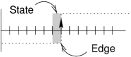
Figure 8: Edge-detecting state

However, in order to effectively express properties containing edges, we need to realize that an edge is detected just before it occurs, as illustrated in Figure 8 That is, $\mathord{\uparrow}A$ becomes true in the state where $A$ is false.

Thus, our formula has a problem: we start testing $P$ before the edge in $Q$ because this is when we detect $\mathord{\uparrow}Q$. We need to fix this by testing $P$ after the edge in $Q$:

$$\mathord{\Box}(\mathord{\uparrow}Q\land\mathord{\Diamond}\mathord{\uparrow}R\Rightarrow\mathord{\circ}(\lnot P\mathbin{\mathcal{U}}\mathord{\uparrow}R))$$

We fixed the above problem but introduced another: the new formula does not work correctly when $\mathord{\uparrow}Q$ and $\mathord{\uparrow}P$ occur simultaneously. This happens because we make sure that $\mathord{\uparrow}R$ occurs one state too early. We need to fix the antecedent by making sure that the interval is non-empty:

$$\mathord{\Box}(\mathord{\uparrow}Q\land\lnot\mathord{\uparrow}R\land\mathord{\Diamond}\mathord{\uparrow}R\Rightarrow\mathord{\circ}(\lnot P\mathbin{\mathcal{U}}\mathord{\uparrow}R))$$

Unfortunately, the resulting formula is still incorrect: if $P$ and $\mathord{\uparrow}R$ occur simultaneously, then that occurrence of $P$ will be ignored since $\mathord{\uparrow}R$ is detected in the state before the edge. This is not the intended behavior as the state before the edge is considered part of the interval. We need to fix it one more time:

$$\mathord{\Box}(\mathord{\uparrow}Q\land\lnot\mathord{\uparrow}R\land\mathord{\Diamond}\mathord{\uparrow}R\Rightarrow\mathord{\circ}\lnot(\lnot\mathord{\uparrow}R\mathbin{\mathcal{U}}P))$$

or better yet:

$$\mathord{\Box}(\mathord{\uparrow}Q\land\lnot\mathord{\uparrow}R\land\mathord{\Diamond}\mathord{\uparrow}R\Rightarrow\mathord{\circ}(\mathord{\uparrow}R\mathbin{\mathcal{P}}P))$$

Note that we can avoid many complications of the sort discussed above if we add the “previous” modality, $Y$. Using this new operator, we can detect edges just after they occur: $a\land\lnot Ya$ (see Figure 8). Although having the “previous” operator can potentially simplify a number of properties, it is currently not supported by SPIN.

4 Closure Under Stuttering

The extension of the pattern system presented in Section 3, is an important development, and we hope that the resulting patterns provide real value to the end user. Still, can practitioners use our extensions directly, without worrying about any unexpected behavior?

The patterns that we have created in the previous section contain the “next” operator. Thus, they may not be closed under stuttering. Intuitively, a formula is closed under stuttering when its interpretation is not modified by transitions that leave the system in the same state. For example, a formula $\mathord{\Box}a$ is closed under stuttering because no matter how much we repeat states, we cannot change the value of $a$. On the other hand, the formula $\circ a$ is not closed under stuttering. We can see that by considering a state sequence in which $a$ is true in the first state and false in the second. Then $\circ a$ is false if we evaluate it on this sequence, and true if we repeat the first state.

Closure under stuttering is an essential property of temporal formulas to ensure basic separation between abstraction levels and to enable powerful partial-order reduction algorithms utilized in mechanized checking, e.g. [8]. This property can be easily guaranteed for a subset of LTL that does not include the “next” operator [10]; however, events cannot be expressed in this subset. Determining whether an LTL formula is closed under stuttering is hard: the problem has been shown to be PSPACE-complete [17]. A computationally feasible algorithm which can identify a subclass of closed under stuttering formulas has been proposed in [7] but have not yet been implemented; without an implementation, one can not say how often the subclass of formulas identified by the algorithm is encountered in practice. Several temporal logics that try to solve the problem have been proposed. Such logics, e.g. TLA [10] and MTL [14], restrict the language so that all formulas expressed in it are, by definition, closed under stuttering. However, it is not clear if these languages are expressive enough for practical use.

In this section we briefly present a set of theorems that allow syntactic reasoning about closure under stuttering in LTL formulas and show how to apply them to our extensions of the pattern system. For a more complete treatment of closure under stuttering, please refer to [18, 19].

4.1 Formal Definition

The notation below is adopted from [6]. A sequence (or string) is a succession of elements joined by semicolons. For example, we write the sequence comprised of the first five natural numbers, in order, as $0;1;2;3;4\$ or, more compactly, as $0;..5$ (note the left-closed, right-open interval). We can obtain an item of the sequence by subscripting: $(0;2;4;5)_{2}=4$. When the subscript is a sequence, we obtain a subsequence: $(0;3;1;5;8;2)_{1;2;3}=(0;3;1;5;8;2)_{1;..4}=3;1;5$. A state is modeled by a function that maps variables to their values, so the value of variable $a$ in state $s_{0}$ is $s_{0}(a)$. We denote the set of all infinite sequences of states as $\mathit{stseq}$, and the set of natural numbers as $\mathbb{N}$.

We say that an LTL formula $F$ is closed under stuttering when its interpretation remains the same under state sequences that differ only by repeated states. We denote an interpretation of formula $F$ in state sequence $s$ as $s\mathopen{[\![}F\mathclose{]\!]}$, and a closed under stuttering formula as $\mathopen{\ll}F\mathclose{\gg}$. $\mathopen{\ll}F\mathclose{\gg}$ is formally defined as follows:

Definition 1

$\mathopen{\ll}F\mathclose{\gg}\mathbin{\mbox{\large$\boldsymbol{=}$}}\mathord{\forall}s\in\mathit{stseq}\cdot\mathord{\forall}i\in\mathbb{N}\cdot s\mathopen{[\![}F\mathclose{]\!]}=(s_{0;..i};s_{i};s_{i;..\infty})\mathopen{[\![}F\mathclose{]\!]}$

In other words, given any state sequence $s$, we can repeat any of its states without changing the interpretation of $F$. Note that $s_{0;..i};s_{i};s_{i;..\infty}$ is a sequence of states that differs from $s$ only by repeating a state $s_{i}$.

4.2 Properties

Here we present several theorems that allow syntactic reasoning about closure under stuttering. First, we note that $\mathord{\downarrow}$ and $\mathord{\uparrow}$ can be used interchangeably when analyzing properties of the form

$$\mathopen{\ll}A\mathclose{\gg}\Rightarrow f(\mathord{\uparrow}A)$$

Thus, in what follows we will only discuss the $\mathord{\uparrow}$-edge.

We start with a few generic properties of closure under stuttering:

$$(\mathit{const}(a)\lor\mathit{var}(a)) \Rightarrow \mathopen{\ll}a\mathclose{\gg}$$ (4)

$$\mathopen{\ll}A\mathclose{\gg} = \mathopen{\ll}\lnot A\mathclose{\gg}$$ (5)

$$(\mathopen{\ll}A\mathclose{\gg}\land\mathopen{\ll}B\mathclose{\gg}) \Rightarrow \mathopen{\ll}A\land B\mathclose{\gg}$$ (6)

$$(\mathopen{\ll}A\mathclose{\gg}\land\mathopen{\ll}B\mathclose{\gg}) \Rightarrow \mathopen{\ll}A\lor B\mathclose{\gg}$$ (7)

$$(\mathopen{\ll}A\mathclose{\gg}\land\mathopen{\ll}B\mathclose{\gg}) \Rightarrow \mathopen{\ll}A\Rightarrow B\mathclose{\gg}$$ (8)

$$\mathopen{\ll}A\mathclose{\gg} \Rightarrow \mathopen{\ll}\mathord{\Box}A\mathclose{\gg}$$ (9)

$$\mathopen{\ll}A\mathclose{\gg} \Rightarrow \mathopen{\ll}\mathord{\Diamond}A\mathclose{\gg}$$ (10)

$$(\mathopen{\ll}A\mathclose{\gg}\land\mathopen{\ll}B\mathclose{\gg}) \Rightarrow \mathopen{\ll}A\mathbin{\mathcal{U}}B\mathclose{\gg}$$ (11)

For example, (4)-(8) indicate that all propositional formulas are closed under stuttering. The above properties do not include reasoning about formulas that contain the “next” operator. For those, we need the following theorem, proven in [18]:

Theorem 4.1 (cus-main-thm)

$$\begin{array}[]{ll}&(\mathopen{\ll}A\mathclose{\gg}\land\mathopen{\ll}B\mathclose{\gg}\land\mathopen{\ll}C\mathclose{\gg}\land\mathopen{\ll}D\mathclose{\gg}\land\mathopen{\ll}E\mathclose{\gg}\land\mathopen{\ll}F\mathclose{\gg})\\ \Rightarrow&\\ &\mathopen{\ll}(\lnot\mathord{\uparrow}A\lor\mathord{\circ}B\lor C)\mathbin{\mathcal{U}}(\mathord{\uparrow}D\land\mathord{\circ}E\land F)\mathclose{\gg}\end{array}$$

This theorem establishes an important relationship between the “next” operator, edges, and closure under stuttering. It gives rise to a number of corollaries that we found to be useful in practice.

Property 1

$$(\mathopen{\ll}A\mathclose{\gg}\land\mathopen{\ll}B\mathclose{\gg}\land\mathopen{\ll}C\mathclose{\gg})\Rightarrow\mathopen{\ll}\mathord{\Diamond}(\mathord{\uparrow}A\land\mathord{\circ}B\land C)\mathclose{\gg}$$

If we take $B=\top$ or $C=\top$ respectively, we obtain two simplified versions:

$$(\mathopen{\ll}A\mathclose{\gg}\land\mathopen{\ll}B\mathclose{\gg})\Rightarrow\mathopen{\ll}\mathord{\Diamond}(\mathord{\uparrow}A\land B)\mathclose{\gg}$$

and

$$(\mathopen{\ll}A\mathclose{\gg}\land\mathopen{\ll}B\mathclose{\gg})\Rightarrow\mathopen{\ll}\mathord{\Diamond}(\mathord{\uparrow}A\land\mathord{\circ}B)\mathclose{\gg}$$

These formulas represent an existence property: an event $\mathord{\uparrow}A$ must happen and then $B$, evaluated before or after the event, should hold.

Property 2

$$(\mathopen{\ll}A\mathclose{\gg}\land\mathopen{\ll}B\mathclose{\gg}\land\mathopen{\ll}C\mathclose{\gg})\Rightarrow\mathopen{\ll}\mathord{\Box}(\mathord{\uparrow}A\Rightarrow\mathord{\circ}B\lor C)\mathclose{\gg}$$

is similar to Property 1. Its two simplified versions are

$$(\mathopen{\ll}A\mathclose{\gg}\land\mathopen{\ll}B\mathclose{\gg})\Rightarrow\mathopen{\ll}\mathord{\Box}(\mathord{\uparrow}A\Rightarrow B)\mathclose{\gg}$$

and

$$(\mathopen{\ll}A\mathclose{\gg}\land\mathopen{\ll}B\mathclose{\gg})\Rightarrow\mathopen{\ll}\mathord{\Box}(\mathord{\uparrow}A\Rightarrow\mathord{\circ}B)\mathclose{\gg}$$

They express a universality property: whenever an event $\mathord{\uparrow}A$ happens, $B$, evaluated right before or right after the event, will hold.

4.3 Closure Under Stuttering and the Pattern System

All properties of Figures 3-7 have been shown to be closed under stuttering. This was done using general rules of logic and properties identified above. For example, consider checking a property

$$\mathord{\Box}(\mathord{\uparrow}Q\land\lnot\mathord{\uparrow}R\land\mathord{\Diamond}\mathord{\uparrow}R\Rightarrow\mathord{\circ}\lnot(\lnot\mathord{\uparrow}R\mathbin{\mathcal{U}}P))$$

for closure under stuttering. The proof goes as follows:

	$\mathopen{\ll}\mathord{\Box}(\mathord{\uparrow}Q\land\lnot\mathord{\uparrow}R\land\mathord{\circ}\mathord{\Diamond}\mathord{\uparrow}R\Rightarrow\mathord{\circ}\lnot(\lnot\mathord{\uparrow}R\mathbin{\mathcal{U}}P))\mathclose{\gg}$
	by rules of logic and LTL
$\mathbin{\mbox{\large$\boldsymbol{=}$}}$	$\mathopen{\ll}\mathord{\Box}(\mathord{\uparrow}Q\land\lnot\mathord{\uparrow}R\Rightarrow\mathord{\circ}(\lnot(\lnot\mathord{\uparrow}R\mathbin{\mathcal{U}}P)\lor\lnot\mathord{\Diamond}\mathord{\uparrow}R))\mathclose{\gg}$
	by definition of $\mathord{\uparrow}$ and rules of logic
$\mathbin{\mbox{\large$\boldsymbol{=}$}}$	$\mathopen{\ll}\mathord{\Box}(\mathord{\uparrow}Q\land(R\lor\mathord{\circ}\lnot R)\Rightarrow\mathord{\circ}(\lnot(\lnot\mathord{\uparrow}R\mathbin{\mathcal{U}}P)\lor\lnot\mathord{\Diamond}\mathord{\uparrow}R))\mathclose{\gg}$
	again, by rules of logic and LTL
$\mathbin{\mbox{\large$\boldsymbol{=}$}}$	$\mathopen{\ll}\mathord{\Box}((\mathord{\uparrow}Q\land R\Rightarrow\mathord{\circ}(\lnot(\lnot\mathord{\uparrow}R\mathbin{\mathcal{U}}P)\lor\lnot\mathord{\Diamond}\mathord{\uparrow}R)))\land\mbox{}$
	$\phantom{\mathopen{\ll}}\mathord{\Box}(\mathord{\uparrow}Q\Rightarrow\mathord{\circ}(\lnot(\lnot\mathord{\uparrow}R\mathbin{\mathcal{U}}P)\lor\lnot\mathord{\Diamond}\mathord{\uparrow}R\lor R))\mathclose{\gg}$
	distribute $\mathopen{\ll}{}\mathclose{\gg}$ over the main conjunction
$\mathbin{\mbox{\large$\boldsymbol{\Leftarrow}$}}$	$\mathopen{\ll}\mathord{\Box}((\mathord{\uparrow}Q\land R\Rightarrow\mathord{\circ}(\lnot(\lnot\mathord{\uparrow}R\mathbin{\mathcal{U}}P)\lor\lnot\mathord{\Diamond}\mathord{\uparrow}R)))\mathclose{\gg}\land\mbox{}$
	$\mathopen{\ll}\mathord{\Box}(\mathord{\uparrow}Q\Rightarrow\mathord{\circ}(\lnot(\lnot\mathord{\uparrow}R\mathbin{\mathcal{U}}P)\lor\lnot\mathord{\Diamond}\mathord{\uparrow}R\lor R))\mathclose{\gg}$
	we can use now Property 2 on both conjuncts
$\mathbin{\mbox{\large$\boldsymbol{\Leftarrow}$}}$	$\mathopen{\ll}Q\mathclose{\gg}\land\mathopen{\ll}R\mathclose{\gg}\land\mathopen{\ll}\lnot(\lnot\mathord{\uparrow}R\mathbin{\mathcal{U}}P)\lor\lnot\mathord{\Diamond}\mathord{\uparrow}R\mathclose{\gg}\land\mbox{}$
	$\mathopen{\ll}Q\mathclose{\gg}\land\mathopen{\ll}\lnot(\lnot\mathord{\uparrow}R\mathbin{\mathcal{U}}P)\lor\lnot\mathord{\Diamond}\mathord{\uparrow}R\lor R\mathclose{\gg}$
	by rules of logic, (5) and (6)
$\mathbin{\mbox{\large$\boldsymbol{\Leftarrow}$}}$	$\mathopen{\ll}Q\mathclose{\gg}\land\mathopen{\ll}R\mathclose{\gg}\land\mathopen{\ll}\lnot\mathord{\uparrow}R\mathbin{\mathcal{U}}P\mathclose{\gg}\land\mathopen{\ll}\mathord{\Diamond}\mathord{\uparrow}R\mathclose{\gg}\land\mbox{}$
	$\mathopen{\ll}Q\mathclose{\gg}\land\mathopen{\ll}\lnot\mathord{\uparrow}R\mathbin{\mathcal{U}}P\mathclose{\gg}\land\mathopen{\ll}\mathord{\Diamond}\mathord{\uparrow}R\mathclose{\gg}\land\mathopen{\ll}R\mathclose{\gg}$
	by Theorem 4.1 and Property 1 we get
$\mathbin{\mbox{\large$\boldsymbol{\Leftarrow}$}}$	$\mathopen{\ll}Q\mathclose{\gg}\land\mathopen{\ll}R\mathclose{\gg}\land\mathopen{\ll}R\mathclose{\gg}\land\mathopen{\ll}P\mathclose{\gg}\land\mathopen{\ll}R\mathclose{\gg}$

We have thus proved that

$$(\mathopen{\ll}P\mathclose{\gg}\land\mathopen{\ll}Q\mathclose{\gg}\land\mathopen{\ll}R\mathclose{\gg})\Rightarrow\mathopen{\ll}\mathord{\Box}(\mathord{\uparrow}Q\land\lnot\mathord{\uparrow}R\land\mathord{\Diamond}\mathord{\uparrow}R\Rightarrow\mathord{\circ}\lnot(\lnot\mathord{\uparrow}R\mathbin{\mathcal{U}}P))\mathclose{\gg}$$

Although the property is fairly complicated, the proof is not long, is completely syntactic, and each step in the proof is easy. Such a proof can potentially be performed by a theorem-prover with minimal help from the user.

As we noted earlier, we did not extend all patterns to include events. The reason is that Precedence Chain, Response Chain and Constrained Chain were not closed under stuttering even in their state-based formulations. Consider, for example, the Response Chain pattern under the Global scope, formalized as

$$\mathord{\Box}((S\land\mathord{\circ}\mathord{\Diamond}T)\Rightarrow\mathord{\circ}\mathord{\Diamond}(T\land\mathord{\Diamond}P))$$

When we evaluate this formula on the state sequence $s$:

$\begin{array}[]{lcccl}&s_{0}&s_{1}&s_{2}&\cdots\\ S&\top&\bot&\bot&\cdots\\ T&\top&\bot&\bot&\cdots\\ P&\bot&\bot&\bot&\cdots\end{array}$

we get $\top$ because the antecedent is always $\bot$. However, if we stutter the first state $s_{0}$, we get the sequence $s_{0};s$:

$\begin{array}[]{lccccl}&s_{0}&s_{0}&s_{1}&s_{2}&\cdots\\ S&\top&\top&\bot&\bot&\cdots\\ T&\top&\top&\bot&\bot&\cdots\\ P&\bot&\bot&\bot&\bot&\cdots\end{array}$

The interpretation of the formula on this sequence is now $\bot$ because the antecedent is $\top$ and the consequent is $\bot$ (since $\mathord{\Diamond}P$ is always $\bot$). As stuttering causes a change in the interpretation of the formula, we can conclude that the formula is not closed under stuttering.

5 Conclusion

In this paper we developed a concept of edges and used it to extend the pattern-based system of Dwyer et. al. to reasoning about events. We have also presented a set of theorems that enable the syntax-based analysis of a large class of formulas for closure under stuttering. This class includes all LTL formulas of the patterns that appeared in this paper. Since research shows that patterns account for 90% of the temporal properties that have been specified so far [4], we believe that our approach is highly applicable to practical problems.

The goal of the pattern-based approach is to enable practitioners to easily codify complex properties into temporal logic. The extensions presented in this paper allow them to express events easily and effectively, without worrying about closure under stuttering. We hope that this work has moved us, as a community, one step closer to making automatic verification more widely usable.

Appendix 0.A Properties of Edges

We list a few representative properties of edges here. Their proofs appear in [18]. [18] also contains a comprehensive study of the concept of edges.

Edges are related:

$$\mathord{\uparrow}\lnot A = \mathord{\downarrow}A$$ (12)

$$\mathord{\downarrow}\lnot A = \mathord{\uparrow}A$$ (13)

$$\mathord{\updownarrow}\lnot A = \mathord{\updownarrow}A$$ (14)

Edges interact with the boolean operators as follows:

$$\mathord{\uparrow}(A\land B) = (\mathord{\uparrow}A\land\mathord{\circ}B)\lor(\mathord{\uparrow}B\land\mathord{\circ}A)$$ (15)

$$\mathord{\uparrow}(A\lor B) = (\mathord{\uparrow}A\land\lnot B)\lor(\mathord{\uparrow}B\land\lnot A)$$ (16)

$$\mathord{\downarrow}(A\land B) = (\mathord{\downarrow}A\land B)\lor(\mathord{\downarrow}B\land A)$$ (17)

$$\mathord{\downarrow}(A\lor B) = (\mathord{\downarrow}A\land\mathord{\circ}\lnot B)\lor(\mathord{\downarrow}B\land\lnot\mathord{\circ}A)$$ (18)

Edges interact with each other:

$$\mathord{\downarrow}\mathord{\downarrow}A = \mathord{\downarrow}A$$ (19)

$$\mathord{\downarrow}\mathord{\uparrow}A = \mathord{\uparrow}A$$ (20)

$$\mathord{\uparrow}\mathord{\downarrow}A = \mathord{\circ}\mathord{\downarrow}A$$ (21)

$$\mathord{\uparrow}\mathord{\uparrow}A = \mathord{\circ}\mathord{\uparrow}A$$ (22)

Edges interact with temporal operators as follows:

$$\mathord{\uparrow}\mathord{\circ}A = \mathord{\circ}\mathord{\uparrow}A$$ (23)

$$\mathord{\downarrow}\mathord{\circ}A = \mathord{\circ}\mathord{\downarrow}A$$ (24)

$$\mathord{\uparrow}\mathord{\Box}A = \mathord{\uparrow}A\land\mathord{\circ}\mathord{\Box}A$$ (25)

$$\mathord{\downarrow}\mathord{\Box}A = \bot$$ (26)

$$\mathord{\uparrow}\mathord{\Diamond}A = \bot$$ (27)

$$\mathord{\downarrow}\mathord{\Diamond}A = \mathord{\downarrow}A\land\mathord{\circ}\mathord{\Box}\lnot A$$ (28)

$$\mathord{\uparrow}(A\mathbin{\mathcal{U}}B) = \lnot(A\lor B)\land\mathord{\circ}(A\mathbin{\mathcal{U}}B)$$ (29)

$$\mathord{\downarrow}(A\mathbin{\mathcal{U}}B) = B\land\lnot\mathord{\circ}(A\mathbin{\mathcal{U}}B)$$ (30)

References

• [1] A. Bernstein and P. K. Harter. Proving real time properties of programs with temporal logic. In Proceedings of the Eight Symposium on Operating Systems Principles, pages 1–11. ACM, 1981.
• [2] E.M. Clarke, E.A. Emerson, and A.P. Sistla. “Automatic Verification of Finite-State Concurrent Systems Using Temporal Logic Specifications”. ACM Transactions on Programming Languages and Systems, 8(2):244–263, April 1986.
• [3] Matthew B. Dwyer, George S. Avrunin, and James C. Corbett. “Property Specification Patterns for Finite-state Verification”. In Proceedings of 2nd Workshop on Formal Methods in Software Practice, March 1998.
• [4] Matthew B. Dwyer, George S. Avrunin, and James C. Corbett. “Patterns in Property Specifications for Finite-State Verification”. In Proceedings of 21st International Conference on Software Engineering, May 1999.
• [5] B. T. Hailpern and S. S. Owicki. Modular verification of computer communication protocols. IEEE Transactions on Communication, 1(COM-31):56–68, 1983.
• [6] Eric C. R. Hehner. A Practical Theory of Programming. Texts and Monographs in Computer Science. Springer-Verlag, New York, 1993.
• [7] G. J. Holzmann and O. Kupferman. “Not Checking for Closure under Stuttering”. In Proceedings of SPIN’96, 1996.
• [8] G.J. Holzmann. “The Model Checker SPIN”. IEEE Transactions on Software Engineering, 23(5):279–295, May 1997.
• [9] Leslie Lamport. Specifying concurrent program modules. ACM Transactions of Programming Languages and Systems, 5:190–222, 1983.
• [10] Leslie Lamport. “The Temporal Logic of Actions”. ACM Transactions on Programming Languages and Systems, 16:872–923, May 1994.
• [11] Z. Manna and A. Pnueli. “Tools and Rules for the Practicing Verifier”. Technical Report STAN-CS-90-1321, Department of Computer Science, Stanford University, 1990. Appeared in Carnegie Mellon Computer Science: A 25 year Commemorative.
• [12] Z. Manna and A. Pnueli. The Temporal Logic of Reactive and Concurrent Systems. Springer-Verlag, 1992.
• [13] K.L. McMillan. Symbolic Model Checking. Kluwer Academic, 1993.
• [14] Abdelillah Mokkedem and Dominique Méry. A stuttering closed temporal logic for modular reasoning about concurrent programs. In Temporal Logic: First International Conference, ICTL ’94, number 827 in Lecture Notes in Artificial Intelligence, Berlin, July 1994. Springer-Verlag.
• [15] Kurt M. Olender and Leon J. Osterweil. “Cecil: A Sequencing Constraint Language for Automatic Static Analysis Generation”. IEEE Transactions on Software Engineering, 16(3):268–280, March 1990.
• [16] J. S. Ostroff. Temporal Logic of Real-Time Systems. Advanced Software Development Series. Research Studies Press (John Wiley & Sons), 1990.
• [17] Doron Peled, Thomas Wilke, and Pierre Wolper. “An Algorithmic Approach for Checking Closure Properties of $\omega$-Regular Languages”. In Proceedings of CONCUR ’96: 7th International Conference on Concurrency Theory, August 1996.
• [18] Dimitrie O. Păun. Closure under stuttering in temporal formulas. Master’s thesis, Department of Computer Science, University of Toronto, Toronto, Ontario M5S 3G4, CANADA, 1999. April.
• [19] Dimitrie O. Păun and Marsha Chechik. “Events in Linear-Time Properties”. In Proceedings of 4th International Conference on Requirements Engineering, June 1999.
• [20] Dimitrie O. Păun, Marsha Chechik, and Bernd Biechelle. “Production Cell Revisited”. In Proceedings of SPIN’98, November 1998.