Reconstructing hv-Convex Polyominoes
from Orthogonal Projections

1 Introduction

Tomography is the area of reconstructing objects from projections. In discrete tomography an object $T$ we wish to reconstruct may be a set of cells of a multidimensional grid. We perform measurements of $T$, each one involving a projection that determines the number of cells in $T$ on all lines parallel to the projection’s direction. Given a finite number of such measurements, we wish to reconstruct $T$ or, if unique reconstruction is not possible, to compute any object consistent with these projections. Gardner et al. [7] proved that deciding if there is an object consistent with given measurements is NP-complete, even for three non-parallel projections in the 2D grid.

In this paper we address the case of orthogonal (horizontal and vertical) projections of a 2D grid. A given object $T$, defined as a set of cells in a $m\times n$ grid, can be identified with an $m\times n$ 0-1 matrix, where the 1’s determine the cells of $T$. We will use all three notations: set-theoretic, integer and boolean, whichever is most appropriate in a given context.

The row and column sums of an object $T$ are defined by $\mathit{rowsum}_{i}(T)=\sum_{j}T_{i,j}$ for $i=1,\ldots,m$ and $\mathit{colsum}_{j}(T)=\sum_{i}T_{i,j}$ for $j=1,\ldots,n$. The vectors $\mathit{rowsum}(T)$ and $\mathit{colsum}(T)$ represent the horizontal and vertical projections of $T$. (See Figure 1.)

[0,r,, An object with its row and column sums.] Given two integer vectors ${\bf r}=(r_{1},\dots,r_{m})$ and ${\bf c}=(c_{1},\dots,c_{n})$, a realization of $({\bf r},{\bf c})$ is an object $T$ whose row and column sum vectors are ${\bf r}$ and ${\bf c}$, that is: $\mathit{rowsum}(T)={\bf r}$ and $\mathit{colsum}(T)={\bf c}$. In the reconstruction problem, given $({\bf r},{\bf c})$, we wish to find a realization $T$ of $({\bf r},{\bf c})$, or to report failure if such $T$ does not exist. The corresponding decision problem is called the consistency problem.

Properties of 0-1 matrices with given row and column sums have been studied in the literature since 1950’s. We refer the reader to the work of Ryser [9], or to an excellent survey by Brualdi [4]. Ryser presents an $O(mn)$ algorithm for the reconstruction problem. In fact, the realizations constructed by his algorithm can be represented and computed in time $O(m+n)$.

For many objects, the orthogonal projections do not provide sufficient information for unique reconstruction. In this case, additional information about the object’s structure could either lead to a unique realization, or at least substantially reduce the number of alternative solutions. Some research has been done on polyominoes, which are connected objects. More formally, we associate with an object $T$ a graph, whose vertices are the cells of $T$, and edges join adjacent cells: $((i,j),(i^{\prime},j^{\prime}))$ is an edge iff $|i-i^{\prime}|+|j-j^{\prime}|\leq 1$. If this graph is connected, then $T$ is called a polyomino. Woeginger [10] proved that the consistency problem for polyominoes is NP-complete.

Some geometric properties of polyominoes have been studied too. Call an object $T$ horizontally convex (or h-convex) if the cells in each row $i$ of $T$ are consecutive, that is, if $(i,k),(i,l)\in T$ then $(i,j)\in T$ for all $k\leq j\leq l$. Vertically convex (v-convex) objects are defined analogously. The consistency problem for h-convex objects (whether we require that they are polyominoes or not) is also known to be NP-complete [2].

If $T$ is both h-convex and v-convex, then we say that $T$ is hv-convex. Kuba [8] initiated the study of hv-convex polyominoes and proposed a reconstruction algorithm with exponential worst-case time complexity. Quite surprisingly, as shown later by Barcucci et al [2], the reconstruction problem for hv-convex polyominoes can be solved in polynomial time. The algorithm given in [2] is, however, rather slow; its time complexity is $O(m^{4}n^{4})$. In another paper, Barcucci et al. [3] showed that certain “median” cells of $({\bf r},{\bf c})$ must belong to any hv-convex polyomino realization, and, using this result, they developed an $O(m^{2}n^{2})$-time heuristic algorithm. This new algorithm is not guaranteed to correctly reconstruct an object, although the experiments reported in [3] indicate that for randomly chosen inputs this method is very unlikely to fail.

The main contribution of this paper is an $O(mn\min(m^{2},n^{2}))$-time algorithm for reconstructing hv-convex polyominoes. Our algorithm is several orders of magnitude faster than the best previously known algorithm from [2], and is also much simpler than the algorithms from [2, 3, 8]. In addition, we address a special case of centered hv-convex polyominoes, in which $r_{i}=n$ for some $i$. In other words, at least one row is completely filled with cells. For this case we show that the reconstruction problem can be solved in time $O(m+n)$.

2 hv-Convex Polyominoes

Throughout the paper, without loss of generality, we assume that ${\bf r},{\bf c}$ denote strictly positive row and column sum vectors. We also assume that $\sum_{i}r_{i}=\sum_{j}c_{j}$, since otherwise $({\bf r},{\bf c})$ do not have a realization.

An object $A$ is called an upper-left corner region if $(i+1,j)\in A$ or $(i,j+1)\in A$ implies $(i,j)\in A$. In an analogous fashion we can define other corner regions. By ${\overline{T}}$ we denote the complement of $T$. The definition of hv-convex polyominoes directly implies the following lemma.

Lemma 1

$T$ is an hv-convex polyomino if and only if ${\overline{T}}=A\cup B\cup C\cup D$, where $A$, $B$, $C$, $D$ are disjoint corner regions (upper-left, upper-right, lower-left and lower-right, respectively) such that (i) $(i-1,j-1)\in A$ implies $(i,j)\notin D$, and (ii) $(i-1,j+1)\in B$ implies $(i,j)\notin C$.

Given an hv-convex polyomino $T$ and two row indices $1\leq k,l\leq m$, we say that $T$ is anchored at $(k,l)$ if $(k,1),(l,n)\in T$. The idea of our algorithm is, given $({\bf r},{\bf c})$, to construct a 2SAT expression (a boolean expression in conjunctive normal form with at most two literals in each clause) $F_{k,l}({\bf r},{\bf c})$ with the property that $F_{k,l}({\bf r},{\bf c})$ is satisfiable iff there is an hv-convex polyomino realization $T$ of $({\bf r},{\bf c})$ that is anchored at $(k,l)$. $F_{k,l}({\bf r},{\bf c})$ consists of several sets of clauses, each set expressing a certain property: “Corners” (Cor), “Disjointness” (Dis), “Connectivity” (Con), “Anchors” (Anc), “Lower bound on column sums” (LBC) and “Upper bound on row sums” (UBR).

$$\mathit{Cor} =\bigwedge_{i,j}\left\{\begin{array}[]{*3{rl@{\hspace*{.8em}}}rl}A_{i,j}&\Rightarrow A_{i-1,j}\hfil\hskip 8.00003pt&B_{i,j}&\Rightarrow B_{i-1,j}\hfil\hskip 8.00003pt&C_{i,j}&\Rightarrow C_{i+1,j}\hfil\hskip 8.00003pt&D_{i,j}&\Rightarrow D_{i+1,j}\\[-1.99997pt] A_{i,j}&\Rightarrow A_{i,j-1}\hfil\hskip 8.00003pt&B_{i,j}&\Rightarrow B_{i,j+1}\hfil\hskip 8.00003pt&C_{i,j}&\Rightarrow C_{i,j-1}\hfil\hskip 8.00003pt&D_{i,j}&\Rightarrow D_{i,j+1}\end{array}\right\}$$

$$\mathit{Dis} =\bigwedge_{i,j}\left\{X_{i,j}\Rightarrow{\overline{Y}}_{i,j}\quad\text{: for symbols }X,Y\in{\left\{A,B,C,D\right\}},X\neq Y\right\}$$

$$\mathit{Con} =\bigwedge_{i,j}\left\{A_{i,j}\Rightarrow{\overline{D}}_{i+1,j+1}\hskip 8.00003ptB_{i,j}\Rightarrow{\overline{C}}_{i+1,j-1}\right\}$$

$$\mathit{Anc} ={\overline{A}}_{k,1}\wedge{\overline{B}}_{k,1}\wedge{\overline{C}}_{k,1}\wedge{\overline{D}}_{k,1}\>\wedge\>{\overline{A}}_{l,n}\wedge{\overline{B}}_{l,n}\wedge{\overline{C}}_{l,n}\wedge{\overline{D}}_{l,n}$$

$$\mathit{LBC} =\bigwedge_{i,j}\left\{\begin{array}[]{rl@{\hspace*{2em}}rl}A_{i,j}&\Rightarrow{{\overline{C}}_{i+c_{j},j}}\hfil\hskip 20.00003pt&A_{i,j}&\Rightarrow{{\overline{D}}_{i+c_{j},j}}\\[-1.99997pt] B_{i,j}&\Rightarrow{{\overline{C}}_{i+c_{j},j}}\hfil\hskip 20.00003pt&B_{i,j}&\Rightarrow{{\overline{D}}_{i+c_{j},j}}\end{array}\right\}\quad\wedge\quad\bigwedge_{j}\left\{{\overline{C}}_{c_{j},j}\quad{\overline{D}}_{c_{j},j}\right\}$$

$$\mathit{UBR} =\bigwedge_{j}\left\{\begin{array}[]{rl@{\hspace*{1em}}rl}\bigwedge_{i\leq\min{\left\{k,l\right\}}}&{{\overline{A}}_{i,j}}\Rightarrow B_{i,j+r_{i}}\hfil\hskip 10.00002pt&\bigwedge_{k\leq i\leq l}&{{\overline{C}}_{i,j}}\Rightarrow B_{i,j+r_{i}}\\[-1.99997pt] \bigwedge_{l\leq i\leq k}&{{\overline{A}}_{i,j}}\Rightarrow D_{i,j+r_{i}}\hfil\hskip 10.00002pt&\bigwedge_{\max{\left\{k,l\right\}}\leq i}&{{\overline{C}}_{i,j}}\Rightarrow D_{i,j+r_{i}}\end{array}\right\}$$

Define $F_{k,l}({\bf r},{\bf c})=\mathit{Cor}\wedge\mathit{Dis}\wedge\mathit{Con}\wedge\mathit{Anc}\wedge\mathit{LBC}\wedge\mathit{UBR}$. All literals with indices outside the set ${\left\{1,\dots,m\right\}}\times{\left\{1,\dots,n\right\}}$ are assumed to have value 1.

 Algorithm 1
Input: ${\bf r}\in\Nset^{m}$, ${\bf c}\in\Nset^{n}$
W.l.o.g assume: $\forall i:r_{i}\in[1,n]$, $\forall j:c_{j}\in[1,m]$, $\sum_{i}r_{i}=\sum_{j}c_{j}$ and $m\leq n$.

For	$k,l=1,\dots,m$ do begin
	If $F_{k,l}({\bf r},{\bf c})$ is satisfiable,
	then output $T=\overline{A\cup B\cup C\cup D}$ and halt.
end
output “failure”.

 

Theorem 2

$F_{k,l}({\bf r},{\bf c})$ is satisfiable if and only if $({\bf r},{\bf c})$ have a realization $T$ that is an hv-convex polyomino anchored at $(k,l)$.

Proof  $(\Leftarrow)$ If $T$ is an hv-convex polyomino realization of $({\bf r},{\bf c})$ anchored at $(k,l)$, then let $A,B,C,D$ be the corner regions from Lemma 1. By Lemma 1, $A$, $B$, $C$ and $D$ satisfy conditions (Cor), (Dis) and (Con). Condition (Anc) is true because $T$ is anchored at $(k,l)$. (LBC) and (UBR) hold because $T$ is a realization of $({\bf r},{\bf c})$.

$(\Rightarrow)$ If $F_{k,l}({\bf r},{\bf c})$ is satisfiable, take $T=\overline{A\cup B\cup C\cup D}$. Conditions (Cor), (Dis) and (Con) imply that the sets $A$, $B$, $C$, $D$ satisfy Lemma 1, and thus $T$ is an hv-convex polyomino. Also, by (Anc), $T$ is anchored at $(k,l)$.

It remains to show that $T$ is a realization of $({\bf r},{\bf c})$. Conditions (UBR) and (LBC) imply that $\mathit{rowsum}_{i}(T)\leq r_{i}$ for each row $i$, and $\mathit{colsum}_{j}(T)\geq c_{j}$ for each column $j$. Thus

$$\sum_{i}r_{i}\geq\sum_{i}\mathit{rowsum}_{i}(T)=\sum_{j}\mathit{colsum}_{j}(T)\geq\sum_{j}c_{j}.$$

Since $\sum_{i}r_{i}=\sum_{j}c_{j}$, $T$ must be a realization of $({\bf r},{\bf c})$, and the proof is complete.    $\Box$

Each formula $F_{k,l}({\bf r},{\bf c})$ has size $O(mn)$ and can be computed in time $O(mn)$. Since 2SAT can be solved in linear time [1, 6], we obtain the following result.

Theorem 3

Algorithm 1 solves the reconstruction problem for hv-convex polyominoes in time $O(mn\min(m^{2},n^{2}))$.

An implementation (see [5]) of Algorithm 1 can be made more efficient by reducing the number of choices for $k,l$. First, restrict $k$ to multiples of $c_{1}$, and $l$ to multiples of $c_{n}$. Second, let $m_{1}$ be the largest index for which $r_{1}\leq\dots\leq r_{m_{1}}$, and let $m_{2}$ be the smallest index for which $r_{m_{2}}\geq\dots\geq r_{m}$. It is easy to see that we can assume that $\min{\left\{k,l\right\}}\leq m_{1}$ and $\max{\left\{k,l\right\}}\geq m_{2}$ (see [3].) Analogously we define column indices $n_{1}$ and $n_{2}$. With these restrictions on $k,l$, we run the 2SAT algorithm only $O(\min(m_{1}m_{2}/c_{1}c_{n},n_{1}n_{2}/r_{1}r_{m}))$ times.

One can also remove redundant clauses from formulas $F_{k,l}({\bf r},{\bf c})$. For example, in the clauses (Dis), we only need to state that regions $A\cap B=\emptyset$ and $C\cap D=\emptyset$. The other disjointness relations follow from condition (LBC). Finally, it is not necessary to reconstruct each $F_{k,l}({\bf r},{\bf c})$ from scratch, since only clauses (UBR) and (Anc) depend on $k$ and $l$.

3 Centered hv-Convex Polyominoes

Structure of realizations.  A rectangle $R$ is the intersection of a set of rows and a set of columns, say $R=I\times J$, for $I\subseteq{\left\{1,\dots,m\right\}}$ and $J\subseteq{\left\{1,\dots,n\right\}}$. The rectangle orthogonal to $R$ is $R^{\perp}={\overline{I}}\times{\overline{J}}$, where ${\overline{I}}$ and ${\overline{J}}$ are the complements of $I,J$.

The lemma below follows from the work of Ryser [9] (see also [4]). We include a simple proof for completeness.

Lemma 4

Let $R=I\times J$ be a rectangle such that $\sum_{i\in I}r_{i}\;=\;\sum_{j\notin J}c_{j}+{\left|I\right|}\cdot{\left|J\right|}$. Then each realization $T$ of $({\bf r},{\bf c})$ satisfies $R\subseteq T$ and $R^{\perp}\cap T=\emptyset$.

Proof  If $T$ is a realization of $({\bf r},{\bf c})$ then

$${\left|R\cap T\right|}-{\left|R^{\perp}\cap T\right|} =\sum_{i\in I}\sum_{j\in J}T_{i,j}-\sum_{i\notin I}\sum_{j\notin J}T_{i,j}\;=\;\sum_{i\in I}\sum_{j}T_{i,j}-\sum_{i}\sum_{j\notin J}T_{i,j}$$

$$=\sum_{i\in I}r_{i}-\sum_{j\notin J}c_{j}\;=\;{\left|I\right|}\cdot{\left|J\right|},$$

and therefore $R\subseteq T$ and $R^{\perp}\cap T=\emptyset$.    $\Box$

Representation of hv-convex realizations.  Since we are interested in centered hv-convex realizations, we assume now that $r_{k}=n$, for some row $k$. We could also assume that the row sums satisfy $r_{1}\leq\dots\leq r_{k}$ and $r_{k}\geq\dots\geq r_{m}$, although our algorithm does not use this assumption.

We represent an hv-convex realization as a vector $T=(t_{1},\dots,t_{m})$, where each $t_{i}\in[1,m-r_{i}+1]$ is the smallest $j$ for which $(i,j)\in T$. Thus $(i,j)\in T$ is equivalent to $t_{i}\leq j<t_{i}+r_{i}$. By definition, such realizations satisfy the horizontal convexity and the row-sum conditions. The vertical convexity condition can be written as

$$t_{i+\delta}\leq t_{i}\leq t_{i+\delta}+r_{i+\delta}-r_{i}$$ (VC)

where $\delta=1$ for $i<k$ and $-1$ for $i>k$. The column sums can be expressed by the $t_{i}$ as $\mathit{colsum}_{j}(T)=|{\left\{i{\,:\,}t_{i}\leq j<t_{i}+r_{i}\right\}}|$.

Partial realizations.  Let $X=(t_{p},\dots,t_{q})$, where $(p,q)\neq(1,m)$ and $k\in[p,q]$, be a vector in which $t_{i}\in[1,m-r_{i}+1]$, for each $i$. We call column $j$ unsaturated if $\mathit{colsum}_{j}(X)<c_{j}$, where $\mathit{colsum}_{j}(X)=|{\left\{i{\,:\,}t_{i}\leq j<t_{i}+r_{i}\right\}}|$. Let $\alpha_{X}$ be the first unsaturated column and $\beta_{X}$ the last. (We will omit the subscript $X$ if $X$ is understood from context.) $X$ is called a $[p,q]$-realization (or a partial realization) if it satisfies condition (VC) for $i=p,\dots,q$, and

$$\min{\left\{t_{p},t_{q}\right\}}\leq\alpha \leq\beta<\max{\left\{t_{p}+r_{p},t_{q}+r_{q}\right\}},$$

$$\mathit{colsum}_{j}(X) =c_{j}\quad\mbox{for}\ j\notin[\alpha,\beta].$$

If $\max{\left\{t_{p},t_{q}\right\}}\leq\alpha$ and $\beta<\min{\left\{t_{p}+r_{p},t_{q}+r_{q}\right\}}$, then $X$ is called balanced. Note that in the definition of partial realizations we do not insist that

$$\mathit{colsum}_{j}(X)\leq c_{j} \quad\mbox{\rm for}\;j=\alpha+1,\dots,\beta-1.$$ (1)

We call $X$ valid if it satisfies (1). Clearly, an invalid partial realization cannot be extended to a realization, but to facilitate a linear-time implementation we will verify (1) only for balanced partial realizations.

Our algorithm will attempt to construct a realization row by row in the order of decreasing sums. A $[p,q]$-realization $X$ will be extended to row $p-1$ or $q+1$, whichever has larger sum. Each $X$ has at most two extensions, and it may have two extensions only if it is balanced. The naive approach would be to explore recursively all extensions, but, if the number of balanced realizations is large, it could result in exponential running time. To reduce the number of partial realizations to explore we show, using Lemma 4, that if $({\bf r},{\bf c})$ has any hv-convex realization at all, then each valid balanced $[p,q]$-realization $X$ can be extended to a realization of $({\bf r},{\bf c})$. Therefore when we encounter a valid balanced $[p,q]$-realization, we can discard all other $[p,q]$-realizations. Consequently, we keep at most two partial realizations at each step.

Suppose that either $q=m$ or $r_{p-1}\geq r_{q+1}$, and let ${{\mbox{\it lext}}_{p-1}(X)}$, ${{\mbox{\it rext}}_{p-1}(X)}$ be the extensions of $X$ with $t_{p-1}=\alpha$ and $t_{p-1}=\beta-r_{p-1}+1$, respectively. If $X$ is non-balanced, or balanced and valid, ${{\mbox{\it Ext}}_{p-1,q}(X)}$ is the set containing these vectors in ${\left\{{{\mbox{\it lext}}_{p-1}(X)},{{\mbox{\it rext}}_{p-1}(X)}\right\}}$ which are $[p-1,q$]-realizations. If $X$ is balanced but not valid then ${{\mbox{\it Ext}}_{p-1,q}(X)}=\emptyset$. Analogously we define the set ${{\mbox{\it Ext}}_{p,q+1}(X)}$ for the case when $p=1$ or $r_{q+1}\geq r_{p-1}$.

 Algorithm 2 (See Fig. 1)
Input: ${\bf r}\in\Nset^{m}$, ${\bf c}\in\Nset^{n}$
W.l.o.g. assume: $\forall i:r_{i}\in[1,n]$, $\forall j:c_{j}\in[1,m]$, $\sum_{i}r_{i}=\sum_{j}c_{j}$ and $\exists k:r_{k}=n$.

$t_{k}{\,\leftarrow\,}1$, $X{\,\leftarrow\,}(t_{k})$, ${\bf P}{\,\leftarrow\,}{\left\{X\right\}}$, $(p,q){\,\leftarrow\,}(k,k)$,
While	$(p,q)\neq(1,m)$ do begin
	If	$q=m$ or $r_{p-1}\geq r_{q+1}$ then $p{\,\leftarrow\,}p-1$ else $q{\,\leftarrow\,}q+1$
	If $\exists X\in{\bf P}$ such that $X$ is valid and balanced
	then ${\bf P}{\,\leftarrow\,}{{\mbox{\it Ext}}_{p,q}(X)}$
	else ${\bf P}{\,\leftarrow\,}\bigcup_{X\in{\bf P}}{{\mbox{\it Ext}}_{p,q}(X)}$
end
If ${\bf P}$ contains a realization $T$ then output $T$ else output “failure”.

 

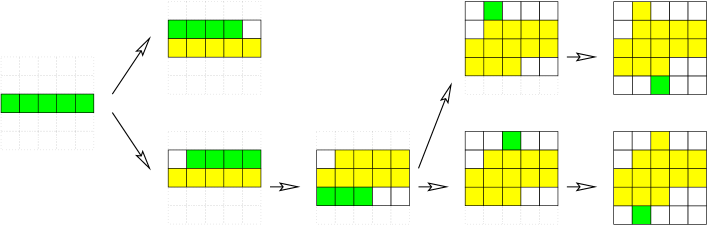
Figure 1: Execution of Algorithm 2 on ${\bf r}=(1,4,5,3,1)$ and ${\bf c}=(2,4,4,2,2)$.

The correctness of Algorithm 2 follows from the following lemma.

Lemma 5

Suppose that $({\bf r},{\bf c})$ has an hv-convex realization. Then, after each step of Algorithm 2, ${\left|{\bf P}\right|}\leq 2$ and there is $X\in{\bf P}$ that can be extended to an hv-convex realization of $({\bf r},{\bf c})$.

Proof  The proof is by induction on $q-p+1$. Denote by ${\bf P}_{p,q}$ the set ${\bf P}$ at the beginning of the while loop. The lemma holds trivially for $p=q=k$. Assume that it holds for some ${\bf P}_{p,q}$. Without loss of generality, assume that either $q=m$ or $r_{p-1}\geq r_{q+1}$.

Suppose first that ${\bf P}_{p,q}$ contains a valid balanced $[p,q]$-realization $X$. Let $I=[p,q]$, $J=[\alpha_{X},\beta_{X}]$ and $R=I\times J$. Then $\sum_{i\in I}r_{i}=\sum_{j\notin J}c_{j}+{\left|I\right|}\cdot{\left|J\right|}$. By Lemma 4, we get that for each realization $T=(z_{1},\dots,z_{m})$, $R\subseteq T$ and $R^{\perp}\cap T=\emptyset$. If we replace $z_{p},\dots,z_{q}$ by $t_{p},\dots,t_{q}$, we get another realization $T^{\prime}$ that is an extension of $X$. Since $q=m$ or $r_{p-1}\geq r_{q+1}$, $z_{p-1}$ must be either $\alpha_{X}$ or $\beta_{X}-r_{p-1}+1$. Therefore $T^{\prime}$ is an extension of one of ${{\mbox{\it rext}}_{p-1}(X)},{{\mbox{\it lext}}_{p-1}(X)}$. Since ${\bf P}_{p-1,q}={{\mbox{\it Ext}}_{p-1,q}(X)}$, the lemma holds for ${\bf P}_{p-1,q}$.

If ${\bf P}_{p,q}$ does not contain a valid balanced $[p,q]$-realization then, for $X\in{\bf P}_{p,q}$, either $\alpha_{X}<\max{\left\{t_{p},t_{q}\right\}}$ or $\beta_{X}\geq\min{\left\{t_{p}+r_{p},t_{q}+r_{q}\right\}}$. Thus each $X\in{\bf P}_{p,q}$ gives rise to at most one extension in ${\bf P}_{p-1,q}$, so we have ${\left|{\bf P}_{p-1,q}\right|}\leq 2$. Pick $X\in{\bf P}_{p,q}$ that can be extended to a realization $T=(t_{1},\dots,t_{m})$. We can assume $\alpha_{X}<\max{\left\{t_{p},t_{q}\right\}}$, since the other case is symmetric. If $t_{p}\leq\alpha_{X}<t_{q}$, then $t_{p-1}=\alpha_{X}$, and $T$ is an extension of ${{\mbox{\it lext}}_{p-1}(X)}\in{\bf P}_{p-1,q}$. If $t_{q}\leq\alpha_{X}<t_{p}$, then $t_{q+1}=\alpha_{X}$, and thus, by $t_{p-1}\geq t_{q+1}$, we have $t_{p-1}=\beta_{X}-r_{p-1}+1$. Therefore $T$ is an extension of ${{\mbox{\it rext}}_{p-1}(X)}\in{\bf P}_{p-1,q}$.    $\Box$

Linear-time implementation.  A naive implementation of Algorithm 2 takes time $O(mn)$. We show how to reduce the running time to $O(m+n)$.

The computation can be divided into phases, where each phase starts when a valid balanced partial realization $Y$ is encountered. During a phase, for each $X\in{\bf P}$, we store only rows which are not in $Y$, and when the phase ends the new rows are copied into $Y$. We also maintain the indices $\alpha=\alpha_{X}$ and $\beta=\beta_{X}$. Call a column $j$ active if $j\in[\alpha,\beta]$. To keep track of the sums of the active columns, we use two arrays $\mathit{hisum}_{j}$ and $\mathit{losum}_{j}$ which represent, respectively, the column sums of rows $[p,k-1]$ and $[k+1,q]$ in $X$. Only the values of $\mathit{hisum}_{j}$ for $j\in[\alpha_{X},t_{p}-1]\cup[t_{p}+r_{p},\beta_{X}]$ are stored explicitly. For $j=[t_{p},t_{p}+r_{p}-1]$, we know that $\mathit{hisum}_{j}=k-p-1$. When $t_{p}$ increases or $t_{p}+r_{p}$ decreases, we simply fill the new entries with the correct values. The array $\mathit{losum}_{j}$ is maintained analogously. In this way, we can maintain these arrays in total time $O(m+n)$ and we can query $\mathit{colsum}_{j}$ in time $O(1)$, since $\mathit{colsum}_{j}=\mathit{hisum}_{j}+1+\mathit{losum}_{j}$.

It remains to show that condition (1) can be tested in total time $O(m+n)$. We keep the list $A$ of the active columns $j$ in the order of increasing sums. Let $\ell$ be the first column in $A$, that is $c_{\ell}=\min_{j\in[\alpha,\beta]}c_{j}$. Then for a balanced realization $X$, $(\ref{eqn: pq-realization})$ holds iff $q-p+1\leq c_{\ell}$, and thus each verification of $(\ref{eqn: pq-realization})$ takes time $O(1)$. Initially, $A$ can be constructed in time $O(m+n)$ by bucket-sort. Each active column has a pointer to its record in $A$. When we increase $\alpha$ or decrease $\beta$, we simply remove from $A$ the columns that become non-active, at cost $O(1)$ per deletion.

In summary, we obtain the following result.

Theorem 6

Algorithm 2 solves the reconstruction problem for centered hv-convex polyominoes, and it can be implemented in time $O(m+n)$.

4 Final Comments

To speed up Algorithm 1 further, one can explore the fact that the consecutive expressions $F_{k,l}({\bf r},{\bf c})$ differ only very slightly. Thus, an efficient dynamic algorithm for 2SAT could be used to improve the time complexity. The 2SAT problem is closely related to strong connectivity in directed graphs, for which no efficient dynamic algorithms are known. Nevertheless, it may be possible to take advantage of the special structure of the 2SAT instances arising in our algorithm, as well as the fact that the sequence of clause insertions/deletions in $F_{k,l}({\bf r},{\bf c})$ is known in advance.

It would be interesting to investigate polyominoes which are digital images of convex shapes. Call a polyomino $T$ convex if its convex hull does not contain any whole cells outside $T$. How fast can we reconstruct convex polyominoes?

References

- [1] B. Aspvall, M. F. Plass, and R. E. Tarjan. A linear-time algorithm for testing the truth of certain quantified boolean formulas. Information Processing Letters, 8(3):121–123, 1979.
- [2] E. Barcucci, A. Del Lungo, M. Nivat, and R. Pinzani. Reconstructing convex polyominoes from horizontal and vertical projections. Theoretical Computer Science, 155(2):321–347, 1996.
- [3] E. Barcucci, A. Del Lungo, M. Nivat, and R. Pinzani. Medians of polyominoes: a property for the reconstruction. International Journal of Imaging Systems and Technology, 1998. to appear.
- [4] R.A. Brualdi. Matrices of zeros and ones with fixed row and column sum vectors. Linear Algebra and Applications, 33:159–231, 1980.
- [5] P. Couperous and C. Dürr. http://www.icsi.berkeley.edu/~cduerr /Xray.
- [6] S. Even, A. Itai, and A. Shamir. On the complexity of timetable and multicommodity flow problems. SIAM Journal on Computing, 5(4):691–703, 1976.
- [7] R.J. Gardner, P. Gritzmann, and D. Prangenberg. On the computational complexity of reconstructing lattice sets from their X-rays. Technical Report 970.05012, Techn. Univ. München, Fak. f. Math., 1997.
- [8] A. Kuba. The reconstruction of two-directional connected binary patterns from their two orthogonal projections. Computer Vision, Graphics, and Image Processing, 27:249–265, 1984.
- [9] H.J. Ryser. Combinatorial Mathematics. Mathematical Association of America and Quinn & Boden, Rahway, New Jersey, 1963.
- [10] G.J. Woeginger. The reconstruction of polyominoes from their orthogonal projections. Technical Report SFB-65, TU Graz, Graz, Austria, April 1996.