Cascaded Markov Models

Abstract

This paper presents a new approach to partial parsing of context-free structures. The approach is based on Markov Models. Each layer of the resulting structure is represented by its own Markov Model, and output of a lower layer is passed as input to the next higher layer. An empirical evaluation of the method yields very good results for NP/PP chunking of German newspaper texts.

1 Introduction

Partial parsing, often referred to as chunking, is used as a pre-processing step before deep analysis or as shallow processing for applications like information retrieval, messsage extraction and text summarization. Chunking concentrates on constructs that can be recognized with a high degree of certainty. For several applications, this type of information with high accuracy is more valuable than deep analysis with lower accuracy.

We will present a new approach to partial parsing that uses Markov Models. The presented models are extensions of the part-of-speech tagging technique and are capable of emitting structure. They utilize context-free grammar rules and add left-to-right transitional context information. This type of model is used to facilitate the syntactic annotation of the NEGRA corpus of German newspaper texts [Skut et al., 1997].

Part-of-speech tagging is the assignment of syntactic categories (tags) to words that occur in the processed text. Among others, this task is efficiently solved with Markov Models. States of a Markov Model represent syntactic categories (or tuples of syntactic categories), and outputs represent words and punctuation [Church, 1988, DeRose, 1988, and others]. This technique of statistical part-of-speech tagging operates very successfully, and usually accuracy rates between 96 and 97% are reported for new, unseen text.

?) showed that the technique of statistical tagging can be shifted to the next level of syntactic processing and is capable of assigning grammatical functions. These are functions like subject, direct object, head, etc. They mark the function of a child node within its parent phrase.

 

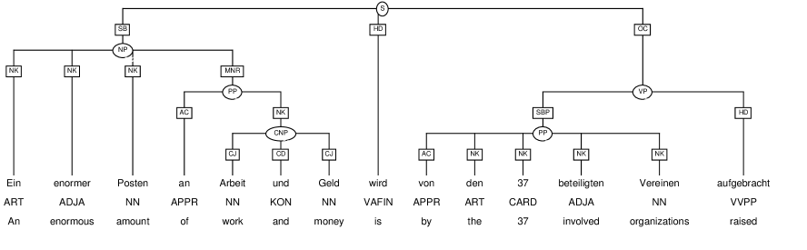
‘A large amount of money and work was raised by the involved organizations’

 

Figure 1: Example sentence and annotation. The structure consists of terminal nodes (words and their parts-of-speech), non-terminal nodes (phrases) and edges (labeled with grammatical functions).

Figure 1 shows an example sentence and its structure. The terminal sequence is complemented by tags (Stuttgart-Tübingen-Tagset, Thielen and Schiller, 1995). Non-terminal nodes are labeled with phrase categories, edges are labeled with grammatical functions (NEGRA tagset).

In this paper, we will show that Markov Models are not restricted to the labeling task (i.e., the assignment of part-of-speech labels, phrase labels, or labels for grammatical functions), but are also capable of generating structural elements. We will use cascades of Markov Models. Starting with the part-of-speech layer, each layer of the resulting structure is represented by its own Markov Model. A lower layer passes its output as input to the next higher layer. The output of a layer can be ambiguous and it is complemented by a probability distribution for the alternatives.

This type of parsing is inspired by finite state cascades which are presented by several authors.

CASS [Abney, 1991, Abney, 1996] is a partial parser that recognizes non-recursive basic phrases (chunks) with finite state transducers. Each transducer emits a single best analysis (a longest match) that serves as input for the transducer at the next higher level. CASS needs a special grammar for which rules are manually coded. Each layer creates a particular subset of phrase types. FASTUS [Appelt et al., 1993] is heavily based on pattern matching. Each pattern is associated with one or more trigger words. It uses a series of non-deterministic finite-state transducers to build chunks; the output of one transducer is passed as input to the next transducer. [Roche, 1994] uses the fix point of a finite-state transducer. The transducer is iteratively applied to its own output until it remains identical to the input. The method is successfully used for efficient processing with large grammars. [Cardie and Pierce, 1998] present an approach to chunking based on a mixture of finite state and context-free techniques. They use NP rules of a pruned treebank grammar. For processing, each point of a text is matched against the treebank rules and the longest match is chosen. Cascades of automata and transducers can also be found in speech processing, see e.g. [Pereira et al., 1994, Mohri, 1997].

Contrary to finite-state transducers, Cascaded Markov Models exploit probabilities when processing layers of a syntactic structure. They do not generate longest matches but most-probable sequences. Furthermore, a higher layer sees different alternatives and their probabilities for the same span. It can choose a lower ranked alternative if it fits better into the context of the higher layer. An additional advantage is that Cascaded Markov Models do not need a “stratified” grammar (i.e., each layer encodes a disjoint subset of phrases). Instead the system can be immediately trained on existing treebank data.

The rest of this paper is structured as follows. Section 2 addresses the encoding of parsing processes as Markov Models. Section 3 presents Cascaded Markov Models. Section 4 reports on the evaluation of Cascaded Markov Models using treebank data. Finally, section 5 will give conclusions.

2 Encoding of Syntactical Information as Markov Models

 

 

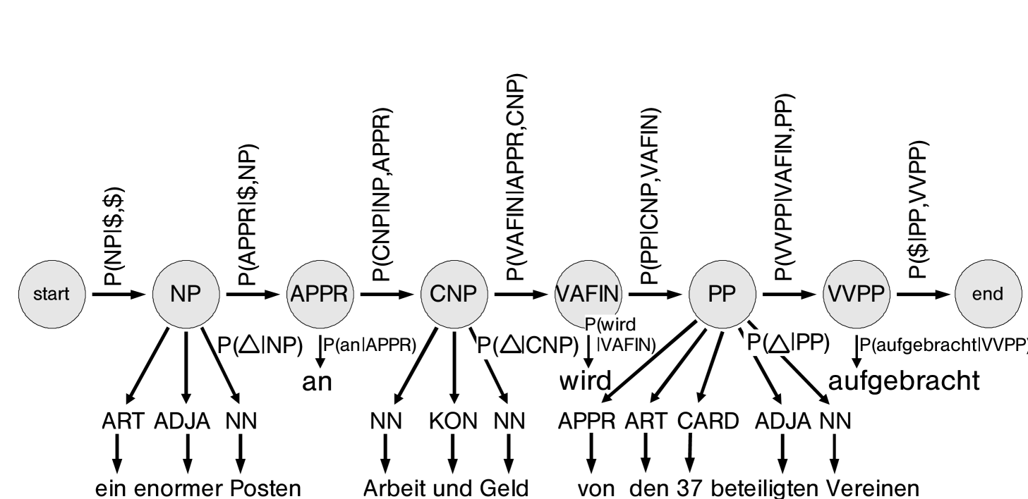
Figure 2: Part of the Markov Models for layer 1 that is used to process the sentence of figure 1. Contrary to part-of-speech tagging, outputs of states may consist of structures with probabilities according to a stochastic context-free grammar.

When encoding a part-of-speech tagger as a Markov Model, states represent syntactic categories and outputs represent words. Contextual probabilities of tags are encoded as transition probabilities of tags, and lexical probabilities of the Markov Model are encoded as output probabilities of words in states.

We introduce a modification to this encoding. States additionally may represent non-terminal categories (phrases). These new states emit partial parse trees (cf. figure 2). This can be seen as collapsing a sequence of terminals into one non-terminal. Transitions into and out of the new states are performed in the same way as for words and parts-of-speech.

Transitional probabilities for this new type of Markov Models can be estimated from annotated data in a way very similar to estimating probabilities for a part-of-speech tagger. The only difference is that sequences of terminals may be replaced by one non-terminal.

Lexical probabilities need a new estimation method. We use probabilities of context-free partial parse trees. Thus, the lexical probability of the state NP in figure 2 is determined by

$$\hskip-14.22636ptP({\sf NP}\rightarrow{\sf ART\ ADJA\ NN},$$

$${\sf ART}\rightarrow{\rm ein},{\sf ADJA}\rightarrow{\rm enormer},{\sf NN}\rightarrow{\rm Posten})$$

$$= P({\sf NP}\rightarrow{\sf ART\ ADJA\ NN})$$

$$\cdot P({\sf ART}\rightarrow{\rm ein})\cdot P({\sf ADJA}\rightarrow{\rm enormer})$$

$$\cdot P({\sf NN}\rightarrow{\rm Posten})$$

Note that the last three probabilities are the same as for the part-of-speech model.

3 Cascaded Markov Models

The basic idea of Cascaded Markov Models is to construct the parse tree layer by layer, first structures of depth one, then structures of depth two, and so forth. For each layer, a Markov Model determines the best set of phrases. These phrases are used as input for the next layer, which adds one more layer. Phrase hypotheses at each layer are generated according to stochastic context-free grammar rules (the outputs of the Markov Model) and subsequently filtered from left to right by Markov Models.

   

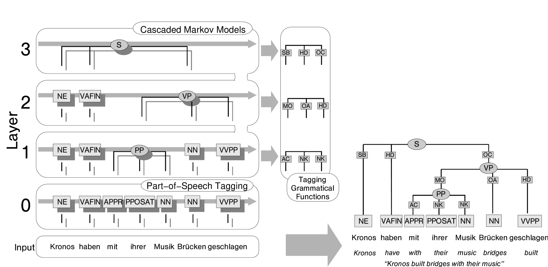
Figure 3: The combined, layered processing model. Starting with part-of-speech tagging (layer 0), possibly ambiguous output together with probabilities is passed to higher layers (only the best hypotheses are shown for clarity). At each layer, new phrases and grammatical functions are added.

Figure 3 gives an overview of the parsing model. Starting with part-of-speech tagging, new phrases are created at higher layers and filtered by Markov Models operating from left to right.

3.1 Tagging Lattices

The processing example in figure 3 only shows the best hypothesis at each layer. But there are alternative phrase hypotheses and we need to determine the best one during the parsing process.

All rules of the generated context-free grammar with right sides that are compatible with part of the sequence are added to the search space. Figure 4 shows an example for hypotheses at the first layer when processing the sentence of figure 1. Each bar represents one hypothesis. The position of the bar indicates the covered words. It is labeled with the type of the hypothetical phrase, an index in the upper left corner for later reference, the negative logarithm of the probability that this phrase generates the terminal yield (i.e., the smaller the better; probabilities for part-of-speech tags are omitted for clarity). This part is very similar to chart entries of a chart parser.

All phrases that are newly introduced at this layer are marked with an asterisk (*). They are produced according to context-free rules, based on the elements passed from the next lower layer. The layer below layer 1 is the part-of-speech layer.

The hypotheses form a lattice, with the word boundaries being states and the phrases being edges. Selecting the best hypothesis means to find the best path from node 0 to the last node (node 14 in the example). The best path can be efficiently found with the Viterbi algorithm [Viterbi, 1967], which runs in time linear to the length of the word sequence. Having this view of finding the best hypothesis, processing of a layer is similar to word lattice processing in speech recognition (cf. Samuelsson, 1997).

Two types of probabilities are important when searching for the best path in a lattice. First, these are probabilities of the hypotheses (phrases) generating the underlying terminal nodes (words). They are calculated according to a stochastic context-free grammar and given in figure 4. The second type are context probabilities, i.e., the probability that some type of phrase follows or precedes another. The two types of probabilities coincide with lexical and contextual probabilities of a Markov Model, respectively.

According to a trigram model (generated from a corpus), the path in figure 4 that is marked grey is the best path in the lattice. Its probability is composed of

$$\begin{array}[]{l}P_{best}=\\ \ P({\sf NP}|\$,\$)P({\sf NP}\Rightarrow^{*}\mbox{\em ein enormer Posten})\\ \ \cdot P({\sf APPR}|\$,{\sf NP})P({\sf APPR}\rightarrow an)\\ \ \cdot P({\sf CNP}|{\sf NP},{\sf APPR})P({\sf CNP}\Rightarrow^{*}\mbox{\em Arbeit und Geld})\\ \ \cdot P({\sf VAFIN}|{\sf APPR},{\sf CNP})P({\sf VAFIN}\rightarrow wird)\\ \end{array}$$

$$\begin{array}[]{l}\ \cdot P({\sf PP}|{\sf CNP},{\sf VAFIN})\\ \hskip 26.00009ptP({\sf PP}\Rightarrow^{*}\mbox{\em von\ den\ 37\ beteiligten\ Vereinen})\\ \ \cdot P({\sf VVPP}|{\sf VAFIN},{\sf PP})P({\sf VVPP}\rightarrow aufgebracht)\\ \ \cdot P(\$|{\sf PP},{\sf VVPP}).\\ \end{array}$$

Start and end of the path are indicated by a dollar sign ($). This path is very close to the correct structure for layer 1. The CNP and PP are correctly recognized. Additionally, the best path correctly predicts that APPR, VAFIN and VVPP should not be attached in layer 1. The only error is the NP ein enormer Posten. Although this is on its own a perfect NP, it is not complete because the PP an Arbeit und Geld is missing. ART, ADJA and NN should be left unattached in this layer in order to be able to create the correct structure at higher layers.

The presented Markov Models act as filters. The probability of a connected structure is determined only based on a stochastic context-free grammar. The joint probabilities of unconnected partial structures are determined by additionally using Markov Models. While building the structure bottom up, parses that are unlikely according to the Markov Models are pruned.

 

                                01234567891011121314   Layer 1 Einenor-merPo-stenanAr-beitundGeldwirdvonden37betei-ligtenVer-einenaufge-bracht1ART        16NP*6.60          17NP*9.68        2ADJA        18AP*10.28        19NP*7.69        3NN          4APPR        20AP*9.25        21PP*6.38        5NN          22CNP*9.05        6KON        7NN        23VP*9.00          8VAFIN        9APPR        24PP*6.22        25AVP*6.88        26PP*10.23          27PP*17.96        10ART        28NP*8.63        29NM*9.23        11CARD        30AP*11.55        31NP*12.24        12ADJA        32NP*11.51        13NN          14VVPP       

 

Figure 4: Phrase hypotheses according to a context-free grammar for the first layer. Hypotheses marked with an asterisk (*) are newly generated at this layer, the others are passed from the next lower layer (layer 0: part-of-speech tagging). The best path in the lattice is marked grey.

3.2 The Method

The standard Viterbi algorithm is modified in order to process Markov Models operating on lattices. In part-of-speech tagging, each hypothesis (a tag) spans exactly one word. Now, a hypothesis can span an arbitrary number of words, and the same span can be covered by an arbitrary number of alternative word or phrase hypotheses. Using terms of a Markov Model, a state is allowed to emit a context-free partial parse tree, starting with the represented non-terminal symbol, yielding part of the sequence of words. This is in contrast to standard Markov Models. There, states emit atomic symbols. Note that an edge in the lattice is represented by a state in the corresponding Markov Model. Figure 2 shows the part of the Markov Model that represents the best path in the lattice of figure 4.

The equations of the Viterbi algorithm are adapted to process a language model operating on a lattice. Instead of the words, the gaps between the words are enumerated (see figure 4), and an edge between two states can span one or more words, such that an edge is represented by a triple $\langle t,t^{\prime},q\rangle$, starting at time $t$, ending at time $t^{\prime}$ and representing state $q$.

We introduce accumulators $\Delta_{t,t^{\prime}}(q)$ that collect the maximum probability of state $q$ covering words from position $t$ to $t^{\prime}$. We use $\delta_{i,j}(q)$ to denote the probability of the deriviation emitted by state $q$ having a terminal yield that spans positions $i$ to $j$. These are needed here as part of the accumulators $\Delta$.

Initialization:

$$\Delta_{0,t}(q)=P(q|q_{s})\delta_{0,t}(q)$$ (1)

Recursion:

$$\Delta_{t,t^{\prime}}(q)=\max_{\langle t^{\prime\prime},t,q^{\prime}\rangle\in\mbox{Lattice}}\Delta_{t^{\prime\prime},t}(q^{\prime})P(q|q^{\prime})\delta_{t,t^{\prime}}(q),~{}~{}~{}$$ (2)

$\mbox{for~{}}1\leq t<T$.
Termination:

$$\max_{Q\in{\cal Q}^{*}}P(Q,{\rm Lattice})=\!\!\!\max_{\langle t,T,q\rangle\in\mbox{Lattice}}\!\!\!\Delta_{t,T}(q)P(q_{e}|q).$$ (3)

Additionally, it is necessary to keep track of the elements in the lattice that maximized each $\Delta_{t,t^{\prime}}(q)$. When reaching time $T$, we get the best last element in the lattice

$$\langle t^{m}_{1},T,q^{m}_{1}\rangle=\mathop{\rm argmax}_{\langle t,T,q\rangle\in\mbox{Lattice}}\Delta_{t,T}(q)P(q_{e}|q).$$ (4)

Setting $t_{0}^{m}=T$, we collect the arguments $\langle t^{\prime\prime},t,q^{\prime}\rangle\in\mbox{Lattice}$ that maximized equation 2 by walking backwards in time:

$$\begin{array}[]{l}\langle t_{i+1}^{m},t_{i}^{m},q_{i+1}^{m}\rangle=\\[4.30554pt] \ \mathop{\rm argmax}\limits_{\langle t^{\prime\prime},t_{i}^{m},q^{\prime}\rangle\in\mbox{Lattice}}\Delta_{t^{\prime\prime},t_{i}^{m}}(q^{\prime})P(q_{i}^{m}|q^{\prime})\delta_{t_{i}^{m},t_{i-1}^{m}}(q_{i})\end{array}$$ (5)

for $i\geq 1$, until we reach $t_{k}^{m}=0$. Now, $q^{m}_{1}\ldots q^{m}_{k}$ is the best sequence of phrase hypotheses (read backwards).

3.3 Passing Ambiguity to the Next Layer

The process can move on to layer 2 after the first layer is computed. The results of the first layer are taken as the base and all context-free rules that apply to the base are retrieved. These again form a lattice and we can calculate the best path for layer 2.

The Markov Model for layer 1 operates on the output of the Markov Model for part-of-speech tagging, the model for layer 2 operates on the output of layer 1, and so on. Hence the name of the processing model: Cascaded Markov Models.

Very often, it is not sufficient to calculate just the best sequences of words/tags/phrases. This may result in an error leading to subsequent errors at higher layers. Therefore, we not only calculate the best sequence but several top ranked sequences. The number of the passed hypotheses depends on a pre-defined threshold $\theta\geq 1$. We select all hypotheses with probabilities $P\geq P_{best}/\theta$. These are passed to the next layer together with their probabilities.

3.4 Parameter Estimation

 

Layer	Sequence
4	S
3	NP							VAFIN	VP
2	ART	ADJA	NN	PP				VAFIN	VP
1	ART	ADJA	NN	APPR	CNP			VAFIN	PP					VVPP
0	ART	ADJA	NN	APPR	NN	KON	NN	VAFIN	APPR	ART	CARD	ADJA	NN	VVPP

	Context-free rules and their frequencies
	S	$\rightarrow$	NP VAFIN VP	(1)	PP	$\rightarrow$	APPR ART CARD ADJA NN	(1)
	NP	$\rightarrow$	ART ADJA NN PP	(1)	ART	$\rightarrow$	Ein	(1)
	PP	$\rightarrow$	APPR CNP	(1)	ADJA	$\rightarrow$	enormer	(1)
	CNP	$\rightarrow$	NN KON NN	(1)	$\cdots$		$\cdots$
	VP	$\rightarrow$	PP VVPP	(1)	VVPP	$\rightarrow$	aufgebracht	(1)

 

Figure 5: Training material generated from the sentence in figure 1. The sequences for layers 0 – 4 are used to estimate transition probabilities for the corresponding Markov Models. The context-free rules are used to estimate the SCFG, which determines the output probabilities of the Markov Models.

Transitional parameters for Cascaded Markov Models are estimated separately for each layer. Output parameters are the same for all layers, they are taken from the stochastic context-free grammar that is read off the treebank.

Training on annotated data is straight forward. First, we number the layers, starting with 0 for the part-of-speech layer. Subsequently, information for the different layers is collected.

Each sentence in the corpus represents one training sequence for each layer. This sequence consists of the tags or phrases at that layer. If a span is not covered by a phrase at a particular layer, we take the elements of the highest layer below the actual layer. Figure 5 shows the training sequences for layers 0 – 4 generated from the sentence in figure 1. Each sentence gives rise to one training sequence for each layer. Contextual parameter estimation is done in analogy to models for part-of-speech tagging, and the same smoothing techniques can be applied. We use a linear interpolation of uni-, bi-, and trigram models.

A stochastic context-free grammar is read off the corpus. The rules derived from the annotated sentence in figure 1 are also shown in figure 5. The grammar is used to estimate output parameters for all Markov Models, i.e., they are the same for all layers. We could estimate probabilities for rules separately for each layer, but this would worsen the sparse data problem.

4 Experiments

This section reports on results of experiments with Cascaded Markov Models. We evaluate chunking precision and recall, i.e., the recognition of kernel NPs and PPs. These exclude prenominal adverbs and postnominal PPs and relative clauses, but include all other prenominal modifiers, which can be fairly complex adjective phrases in German. Figure 7 shows an example of a complex NP and the output of the parsing process.

 

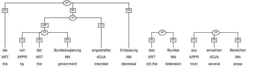
‘the dismissal of the federation from several areas that was intended by the government’

 

Figure 6: Complex German NP and chunker output (postnominal genitive and PP are not attached).

 

NEGRA Corpus: Chunking Results
                    123456789             60708090100        Recall/Precision # Layers96.296.396.496.496.596.596.596.596.5% POS accuracy   Topline Recall min = 72.6% max = 100.0%     $\bullet$  Recall min = 54.0% max = 84.8%     $\circ$  Precision min = 88.3% max = 91.4%                                                                                                                                                                                                                                                                                                                                                                                                                                                                                                                                                                                                                                                                                                                                                                                                                                                                                                                                                                                                                                                                                                                                                                                                                                                                                                            $\bullet$$\bullet$$\bullet$$\bullet$$\bullet$$\bullet$$\bullet$$\bullet$                                                                                                                                                                                                                                                                                                                                                                                                                                                                                                                                                                                                $\circ$$\circ$$\circ$$\circ$$\circ$$\circ$$\circ$$\circ$$\circ$

 

Figure 7: NP/PP chunking results for the NEGRA Corpus. The diagram shows recall and precision depending on the number of layers that are used for parsing. Layer 0 is used for part-of-speech tagging, for which tagging accuracies are given at the bottom line. Topline recall is the maximum recall possible for that number of layers.

For our experiments, we use the NEGRA corpus [Skut et al., 1997]. It consists of German newspaper texts (Frankfurter Rundschau) that are annotated with predicate-argument structures. We extracted all structures for NPs, PPs, APs, AVPs (i.e., we mainly excluded sentences, VPs and coordinations). The version of the corpus used contains 17,000 sentences (300,000 tokens).

The corpus was divided into training part (90%) and test part (10%). Experiments were repeated 10 times, results were averaged. Cross-evaluation was done in order to obtain more reliable performance estimates than by just one test run. Input of the process is a sequence of words (divided into sentences), output are part-of-speech tags and structures like the one indicated in figure 7.

Figure 7 presents results of the chunking task using Cascaded Markov Models for different numbers of layers. Percentages are slightly below those presented by [Skut and Brants, 1998]. But they started with correctly tagged data, so our task is harder since it includes the process of part-of-speech tagging.

Recall increases with the number of layers. It ranges from 54.0% for 1 layer to 84.8% for 9 layers. This could be expected, because the number of layers determines the number of phrases that can be parsed by the model. The additional line for “topline recall” indicates the percentage of phrases that can be parsed by Cascaded Markov Models with the given number of layers. All nodes that belong to higher layers cannot be recognized.

Precision slightly decreases with the number of layers. It ranges from 91.4% for 1 layer to 88.3% for 9 layers.

The $F$-score is a weighted combination of recall $R$ and precision $P$ and defined as follows:

$$F=\frac{(\beta^{2}+1)PR}{\beta^{2}P+R}$$ (6)

$\beta$ is a parameter encoding the importance of recall and precision. Using an equal weight for both ($\beta=1$), the maximum $F$-score is reached for 7 layers ($F=$86.5%).

The part-of-speech tagging accuracy slightly increases with the number of Markov Model layers (bottom line in figure 7). This can be explained by top-down decisions of Cascaded Markov Models. A model at a higher layer can select a tag with a lower probability if this increases the probability at that layer. Thereby some errors made at lower layers can be corrected. This leads to the increase of up to 0.3% in accuracy.

Results for chunking Penn Treebank data were previously presented by several authors [Ramshaw and Marcus, 1995, Argamon et al., 1998, Veenstra, 1998, Cardie and Pierce, 1998]. These are not directly comparable to our results, because they processed a different language and generated only one layer of structure (the chunk boundaries), while our algorithm also generates the internal structure of chunks. But generally, Cascaded Markov Models can be reduced to generating just one layer and can be trained on Penn Treebank data.

5 Conclusion and Future Work

We have presented a new parsing model for shallow processing. The model parses by representing each layer of the resulting structure as a separate Markov Model. States represent categories of words and phrases, outputs consist of partial parse trees. Starting with the layer for part-of-speech tags, the output of lower layers is passed as input to higher layers. This type of model is restricted to a fixed maximum number of layers in the parsed structure, since the number of Markov Models is determined before parsing. While the effects of these restrictions on the parsing of sentences and VPs are still to be investigated, we obtain excellent results for the chunking task, i.e., the recognition of kernel NPs and PPs.

It will be interesting to see in future work if Cascaded Markov Models can be extended to parsing sentences and VPs. The average number of layers per sentence in the NEGRA corpus is only 5; 99.9% of all sentences have 10 or less layers, thus a very limited number of Markov Models would be sufficient.

Cascaded Markov Models add left-to-right context-information to context-free parsing. This contextualization is orthogonal to another important trend in language processing: lexicalization. We expect that the combination of these techniques results in improved models.

We presented the generation of parameters from annotated corpora and used linear interpolation for smoothing. While we do not expect improvements by re-estimation on raw data, other smoothing methods may result in better accuracies, e.g. the maximum entropy framework. Yet, the high complexity of maximum entropy parameter estimation requires careful pre-selection of relevant linguistic features.

The presented Markov Models act as filters. The probability of the resulting structure is determined only based on a stochastic context-free grammar. While building the structure bottom up, parses that are unlikely according to the Markov Models are pruned. We think that a combined probability measure would improve the model. For this, a mathematically motivated combination needs to be determined.

References

- [Abney, 1991] Steven Abney. 1991. Parsing by chunks. In Robert Berwick, Steven Abney, and Carol Tenny, editors, Principle-Based Parsing, Dordrecht. Kluwer Academic Publishers.
- [Abney, 1996] Steven Abney. 1996. Partial parsing via finite-state cascades. In Proceedings of the ESSLLI Workshop on Robust Parsing, Prague, Czech Republic.
- [Appelt et al., 1993] D. Appelt, J. Hobbs, J. Bear, D. J. Israel, and M. Tyson. 1993. FASTUS: a finite-state processor for information extraction from real-world text. In Proceedings of IJCAI-93, Washington, DC.
- [Argamon et al., 1998] Shlomo Argamon, Ido Dagan, and Yuval Krymolowski. 1998. A memory-based approach to learning shallow natural language patterns. In Proceedings of the 17th International Conference on Computational Linguistics COLING-ACL-98), Montreal, Canada.
- [Brants et al., 1997] Thorsten Brants, Wojciech Skut, and Brigitte Krenn. 1997. Tagging grammatical functions. In Proceedings of the Conference on Empirical Methods in Natural Language Processing EMNLP-97, Providence, RI, USA.
- [Cardie and Pierce, 1998] Claire Cardie and David Pierce. 1998. Error-driven pruning of treebank grammars for base noun phrase identification. In Proceedings of the 17th International Conference on Computational Linguistics COLING-ACL-98), Montreal, Canada.
- [Church, 1988] Kenneth Ward Church. 1988. A stochastic parts program and noun phrase parser for unrestricted text. In Proceedings of the Second Conference on Applied Natural Language Processing ANLP-88, pages 136–143, Austin, Texas, USA.
- [DeRose, 1988] Steven J. DeRose. 1988. Grammatical category disambiguation by statistical optimization. Computational Linguistics, 14(1):31–39.
- [Mohri, 1997] Mehryar Mohri. 1997. Finite-state transducers in language and speech processing. Computational Linguistics, 23(2).
- [Pereira et al., 1994] Fernando Pereira, Michael Riley, and Richard Sproat. 1994. Weighted rational transductions and their application to human language processing. In Proceedings of the Workshop on Human Language Technology, San Francisco, CA. Morgan Kaufmann.
- [Ramshaw and Marcus, 1995] Lance A. Ramshaw and Mitchell P. Marcus. 1995. Text chunking using transformation-based learning. In Proceedings of the third Workshop on Very Large Corpora, Dublin, Ireland.
- [Roche, 1994] Emmanuel Roche. 1994. Two parsing algorithms by means of finite state transducers. In Proceedings of the 15th International Conference on Computational Linguistics COLING-94, pages 431–435, Kyoto, Japan.
- [Samuelsson, 1997] Christer Samuelsson. 1997. Extending -gram tagging to word graphs. In Proceedings of the 2nd International Conference on Recent Advances in Natural Language Processing RANLP-97, Tzigov Chark, Bulgaria.
- [Skut and Brants, 1998] Wojciech Skut and Thorsten Brants. 1998. A maximum-entropy partial parser for unrestricted text. In Sixth Workshop on Very Large Corpora, Montreal, Canada.
- [Skut et al., 1997] Wojciech Skut, Brigitte Krenn, Thorsten Brants, and Hans Uszkoreit. 1997. An annotation scheme for free word order languages. In Proceedings of the Fifth Conference on Applied Natural Language Processing ANLP-97, Washington, DC.
- [Thielen and Schiller, 1995] Christine Thielen and Anne Schiller. 1995. Ein kleines und erweitertes Tagset fürs Deutsche. In Tagungsberichte des Arbeitstreffens Lexikon + Text 17./18. Februar 1994, Schloß Hohentübingen. Lexicographica Series Maior, Tübingen. Niemeyer.
- [Veenstra, 1998] Jorn Veenstra. 1998. Fast NP chunking using memory-based learning techniques. In Proceedings of the Eighth Belgian-Dutch Conference on Machine Learning, Wageningen.
- [Viterbi, 1967] A. Viterbi. 1967. Error bounds for convolutional codes and an asymptotically optimum decoding algorithm. In IEEE Transactions on Information Theory, pages 260–269.