Learning Efficient Disambiguation

Khalil Sima’an

ILLC Dissertation Series 1999-02

4cm

For further information about ILLC-publications, please contact
Institute for Logic, Language and Computation
Universiteit van Amsterdam
Plantage Muidergracht 24
1018 TV Amsterdam
phone: +31-20-5256090
fax: +31-20-5255101
e-mail: illc@wins.uva.nl

Learning Efficient Disambiguation

Leren Efficiënt te Desambigueren

(met een samenvatting in het Nederlands)

PROEFSCHRIFT
ter verkrijging van de graad van doctor

aan de Universiteit Utrecht

op gezag van de Rector Magnificus, prof. dr. H.O. Voorma

ingevolge het besluit van het College voor Promoties

in het openbaar te verdedigen

op woensdag 31 maart 1999

des ochtends te 10.30 uur.

door

Khalil Sima’an

geboren op 12 september 1964 te Haifa

Promotoren:	Prof. ir. S. P. J. Landsbergen, Universiteit Utrecht
	Prof. dr. ir. R. J. H. Scha, Universiteit van Amsterdam

This work was partially funded by the Netherlands Organization for Scientific Research (NWO) and the Foundation for Language Technology (STT, Utrecht University). It was facilitated by support from the Institute for Logic, Language and Computation (ILLC) and from the Utrecht Institute of Linguistics (Uil-OTS). Learning efficient disambiguation / Khalil Sima’an.
Thesis, Utrecht University - With summary in Dutch
ISBN 90-73446-88-0
Subject headings: natural language processing/machine learning/probabilistic parsing.
Cover design by Yael Seggev
©  by Khalil Sima’an.

Chapter 1 Introduction

1 A brief summary

Many contemporary performance models of natural language parsing resolve ambiguity by acquiring probabilistic grammars from tree-banks that represent language use in limited domains. Among these performance models, the Data Oriented Parsing (DOP) model represents a memory-based approach to language modeling. The DOP model casts a whole tree-bank, which is assumed to represent the language experience of an adult in some domain, into a probabilistic grammar called Stochastic Tree-Substitution Grammar (STSG).

A remarkable fact about contemporary performance models is their entrenched inefficiency. Despite of their ability to learn from tree-banks, these models do not account for two appealing properties of human language processing: firstly, that more frequent utterances are processed more efficiently, and secondly, that utterances in specific contexts, typical for limited domains of language use, are usually less ambiguous than they are in general contexts. This thesis defends the proposition that the absence of mechanisms that represent these and similar properties is a major source for the inefficiency of performance models. Besides this source of inefficiency of performance models in general, the DOP model in particular suffers from other inveterate sources of inefficiency: the huge STSGs that it acquires and the complexity of disambiguation by means of STSGs.

This thesis studies solutions to the inefficiency of performance models in general and the DOP model in particular. The principal idea for removing these sources of inefficiency is to incorporate “efficiency properties” of human behavior in limited domains of language use, such as the properties stated above, into existing performance models. Efficiency properties can be observed through the statistical biases of the linguistic phenomena that are found in tree-banks that represent limited domains of human language use. These properties can be incorporated into a performance model through the combination of two methods of learning from a domain-specific tree-bank: an off-line method that constrains the recognition-power and the ambiguity of the linguistic annotation of the tree-bank such that it specializes it for the domain, and an on-line performance model that acquires less ambiguous and more efficient probabilistic grammars from that less redundant tree-bank. With this idea as departure point, this thesis studies both on-line and off-line learning of ambiguity resolution in the context of the DOP model. To this end

• it presents a framework for specializing performance models, especially the DOP model, and broad-coverage grammars to limited domains by ambiguity reduction. Ambiguity-reduction specialization takes place off-line by using a tree-bank that is representative of a limited domain of language use.

• it presents deterministic polynomial-time algorithms for parsing and disambiguation under the DOP model for various tasks such as sentence disambiguation and word-graph (speech-recognizer’s output) disambiguation. Crucially, these algorithms have time complexity linear in STSG size. It is noteworthy that prior to the first publication of these algorithms, parsing and disambiguation under the DOP model took place solely by means of inefficient non-deterministic exponential-time algorithms.

• it provides proofs that some actual problems of probabilistic disambiguation under Stochastic Context-Free Grammars and Stochastic Tree-Substitution Grammars are NP-Complete. The most remarkable among these problems is the problem of computing the most probable sentence from a word-graph under a Stochastic Context-Free Grammar (SCFG).

• it reports on an extensive empirical study of the DOP model and the specialization algorithms on two independent domains that feature two languages and two different tasks.

The rest of this chapter presents a brief general introduction to this thesis. Section 2 caters especially to readers who are not familiar with the relevant developments and debates in the field of Computational Linguistics in general and in Corpus-based Linguistics in particular. It pinpoints the present research in the general direction of Computational Linguistics by describing the course of arguments that lead to the evolution of what currently are known as performance models of language. Keywords in this section are: linguistic grammars, parsing, competence models, ambiguity, overgeneration, probabilistic grammars, corpus-based models, learning and performance models. Section 3 provides a short introduction to Data Oriented Parsing. Section 4 discusses shortly the principal subject of this thesis: efficiency of performance models. Section 5 states the problems that this thesis deals with, the hypotheses that it defends, and its contributions. Finally section 6 provides an overview of the other chapters.

2 Ambiguity and performance models

Humans interact in speech and in writing and they are usually able to understand the messages that they exchange. The main problem that keeps the researchers busy in the field of Natural Language Processing (NLP) is how to model this linguistic capacity. Besides the “elevated” scientific interest and curiosity, the research in NLP is also driven and often even financed by “humble” economical interest. Needless to say, it is very attractive to automate tasks in which language plays a central role, e.g. systems that you can command through speech, systems that can have a dialogue with humans in order to provide them with information and services (e.g. time-table information and ticket reservation), systems that translate the European Commission’s lengthy reports simultaneously into fifteen or more languages. In fact, some impoverished systems have already found their way to the market, speech-recognition systems that understand some words and even sentences. However, it is not an exaggeration to say that the field of NLP is a baby that has just discovered that it can stand up.

A major assumption that underlies the research in NLP is that human languages share a common internal structure. This assumption is essential for NLP because it implies that it is possible to capture the many and diverse languages in one single model: the model of human languages. What this model should look like and what methods it should be based on is still a subject of debate in NLP research. However, most NLP researchers agree on the need for a divide-and-conquer modeling strategy: the model of understanding a spoken/written message is divided into a sequence of modules, each dealing with a subtask of linguistic understanding. Examples of these modules are speech-recognition (constructing words from speech signals), morphological analysis (exposing the structure of words), part-of-speech tagging (categorizing words), syntactic analysis (exposing the structure of sentences) and semantic analysis (assigning meanings to sentences). By dividing the complex task into smaller subtasks (with suitable interfaces between the corresponding modules), NLP researchers hope that it will be “easier” to understand and model each of the subtasks separately.

In this thesis we are mostly interested in syntactic analysis, also called parsing. Syntactic analysis is concerned with discovering the internal structures of sentences in order to facilitate the construction of representations of their meaning. The syntax of a sentence is a kind of skeleton that supports its “semantic flesh”. Usually, syntactic analysis is not a goal in itself but rather a kind of fore-play which prepares for semantic analysis.

2.1 Competence and performance models

In the past four decades of computational linguistic research, the major concern has been to develop models that characterize what sentences are grammatical and how the meanings of these sentences are constructed from basic units; these basic units can be seen as the bits and pieces of the syntactic skeleton and the corresponding muscles of the semantic flesh. In this, computational linguistics describes a language as a set of sentences, a set of analyses and a correspondence between these two sets. Usually, this triple is described by a grammar that shows how sentences are constructed from smaller phrases, e.g. verb-phrases and noun-phrases, that are in turn constructed from yet smaller phrases or words. A grammar, thus, allows decomposing or parsing a sentence into its basic units; the process of parsing a sentence using a grammar results in analyses (we also say that the grammar - or a parser that is based on it - assigns analyses to the sentence). Computational linguistics aims at developing the types of grammars that seem most suited for describing natural languages. For this difficult task, the computational linguists had to make an inevitable assumption as to what kind of language use interests them: computational linguists assume that the subject matter of their studies is “idealized” language. The computational linguists refer to the grammars that they develop as competence models of language [Chomsky, 1965], as opposed to performance models of language, i.e. models of “non-idealized” linguistic behavior of humans.

2.2 Overgeneration and undergeneration

The focus of computational linguistics on developing grammatical descriptions resulted in lack of attention for modeling the input-output behavior of the human linguistic system. In applications that involve natural language, grammar engineers try in the first place to develop grammars that bridge the gap between these grammatical descriptions and actual language use. Despite of the immense efforts, these grammars suffer from many problems among which two are most severe: overgeneration and undergeneration. Overgeneration, also known as ambiguity, is the phenomenon that a grammar tends to assign too many analyses to a sentence, most of which are not perceived by humans. Undergeneration, on the other hand, is the phenomenon that a grammar does not assign to a sentence the analyses that are perceived by humans (often the grammar does not assign any analyses at all). In this thesis we will focus on the problem of overgeneration. Next we provide two examples of overgeneration. The first exemplifies this problem in natural language and explains why linguistic grammars do not aim at solving it. And the second example exemplifies why this problem is so severe in linguistic grammars.

Example 1.1

Consider the sentence “John found Mary a nice woman”. It has two different interpretations: John considered Mary to be a nice woman or John found a nice woman for Mary. Most people perceive only one interpretation (often the first). Nevertheless, it is essential that a grammar of English be able to analyze this sentence both ways. Only within enough context and with access to knowledge resources beyond language (world-knowledge), the choice of the right analysis might become clear. Therefore, linguistic competence grammars do not try to select the correct analysis but assign (at least) both analyses to the sentence.

Figure 1: Syntactic analyses

Linguistic grammars assign to the preceding example sentence many other analyses beside these two. Most analyses are not perceived by humans and are a byproduct of the complex grammar rules. An empirical study of this problem [Martin et al., 1987] shows that actual linguistic grammars assign hundreds but even thousands of analyses to the very same sentence. The following example shows how this can happen.

Example 1.2

Consider the two sentences “Max eats pizza with a fork” and “Max eats pizza with meat”. The meanings of both sentences are clear to the reader and the correct syntactic analyses of both sentences are found in figure 1. A competence grammar of English should contain the correct analysis for each of the two sentences. However, this means that such a grammar assigns to each of these sentences at least two analyses: the correct analysis and another analysis that is derived by combining rules that originate from the analysis of the other sentence.

A grammar that undergenerates or overgenerates is not very useful in practice. A system based on such a grammar tends to be brittle and inaccurate. Sentences that are assigned no analyses by the grammar are not understood by the system, and sentences that are assigned too many analyses confuse the system. Therefore, for building a system that involves a serious linguistic task, a grammar engineer must find a way to weed out the wrong analyses from the grammar but keep the correct ones in it. This is important because if the wrong analysis is assigned to a sentence it might result in the wrong meaning. Consider what happens if Max eats the fork and the pizza; this is exactly what happens if the analysis at the right-side of figure 1 is properly adjusted and assigned to the sentence at the left-side of that figure.

It is by no means easy to get rid of overgeneration and undergeneration from a grammar for a serious portion of a natural language. Firstly, it is very hard for a human to keep track of the complex interactions between the many rules of a grammar. And secondly, hacking the grammar to get rid of overgeneration usually results in extreme undergeneration (and vice versa). As a matter of fact, there are no serious natural language grammars out there that do not suffer from overgeneration as well as undergeneration.

2.3 The probabilistic-linguistic approach

A decade and a half ago a different approach to the problem of ambiguity in linguistic grammars revived due to its success in speech-recognition: the probabilistic approach. The slogan of this approach is: allow linguistic grammars to overgenerate but resolve the ambiguities by assigning probabilities to the different analyses of a sentence. Assigning probabilities to the analyses of a sentence enables selecting one analysis: the analysis with the highest probability. In fact, according to the probabilistic approach it is possible to assign probabilities that minimize the chance of committing errors in selecting an analysis. Typically, assigning probabilities to the analyses is achieved by attaching probabilities to the rules of the linguistic grammar, resulting in probabilistic or stochastic linguistic grammars e.g. [Fujisaki, 1984, Fujisaki et al., 1989, Jelinek et al., 1990, Resnik, 1992, Schabes, 1992, Schabes and Waters, 1993]

In one view on the probabilistic approach, the probabilities assigned to a linguistic grammar are considered means for approximating phenomena that the grammar is not aimed at modeling, e.g. broad-context (discourse) dependencies and world-knowledge. The probabilities, thus, constitute averages of many variables that influence the choice of the correct analysis of a sentence. Although this view is valid, it might not do the probabilistic approach full justice. Many researchers believe that the probabilistic approach to language has psychological relevance. A relevant psychological observation here is that humans tend to register frequencies and differences between frequencies. Since probabilistic models employ relative frequencies to estimate probabilities, they can be seen as implementing this observation. In any case, since we are here less interested in psychological studies, we will refrain from discussing them and we refer the interested reader to the discussions provided in [Scha, 1990, Scha, 1992, Bod, 1995a] and the references that they cite.

2.4 The corpus-based approach

Although the probabilistic approach offers linguistic grammars a way out of the ambiguity maze, it does not offer a solution to the problem of developing performance models of language. Linguistic grammars model idealized language use. Extending them with probabilities does not make them suitable for modeling linguistic input-output behavior of humans. Many constructions will be missing from the linguistic grammar and have to be engineered by humans. Moreover, there is a related fundamental question with regard to whether probabilities should be attached to linguistic competence grammar rules in the first place. Generally speaking, probabilities are more meaningful when they are attached to dependencies and relations that are more significant for the task they are employed for. In language modeling, often relations between words, between phrasal-categories and, for some sentences, even between whole constituents are most significant in determining the correct analyses of sentences. Therefore, attaching probabilities to the rules of a linguistic competence grammar is equivalent to attaching them only to a small portion of the linguistic relations that are significant to syntactic and semantic analysis.

A major shift in developing performance models took place less than a decade ago. It can be characterized as a shift from a top-down approach to a bottom-up approach to modeling. Rather than considering the linguistically developed competence models as central to performance models, the bottom-up approach puts collections of real-world data, corpora, at the center of its activity. With the corpus of data at the center, this approach, the corpus-based approach, aims at acquiring or learning from the data a suitable performance model. Crucially, the data is collected in such a way that it is representative of language use in some domain. The data may be annotated with linguistic information, or it may be “raw”. If the data are annotated, the annotation is usually based on linguistic knowledge. This offers a kind of “back-door” where linguistic knowledge enters a performance model. Learning from annotated data is analogous to tutoring (supervising) a novice in some task by showing him examples and their solutions. If the data are “raw”, this is similar to learning from scratch without the help of a supervisor (i.e. unsupervised learning).

By acquiring performance models from corpora, the corpus-based approach offers the hope that the acquired performance models will be better suited for processing new similar data. Another attractive feature, market-wise, of automatic learning of performance models is the independence from manual labor, which is not always available and not always consistent.

Currently, there are different corpus-based methods in linguistics. Some of these methods have been successful in acquiring useful performance models for some (relatively simple) linguistic tasks, e.g. part-of-speech tagging of free text (PoSTagging). Examples of successful corpus-based methods for PoSTagging are Hidden Markov Models (HMMs)  [Bahl and Mercer, 1976, Church, 1988], Transformation-Based Error Driven Learning [Brill, 1994, Brill, 1993], Instance-Based Learning [Daelemans et al., 1996] and Maximum-Entropy Modeling [Ratnaparkhi, 1996]. There are a few more linguistic tasks for which the corpus-based approach currently offers suitable solutions, e.g. morphological analysis, phonological analysis, chunking or recognition of noun-phrases. However, in general, these tasks constitute the less complex subtasks of sentence processing. For the more complex tasks, e.g. syntactic and semantic analysis, none of the contemporary corpus-based approaches can claim similar success yet.

Most contemporary corpus-based methods of syntactic analysis are probabilistic, e.g. [Pereira and Schabes, 1992, Magerman, 1994, Bod, 1995a, Charniak, 1996, Collins, 1996, Collins, 1997, Ratnaparkhi, 1997, Srinivas, 1997, Goodman, 1998]; they acquire both their grammars and the probabilities of the grammars from tree-banks, i.e. corpora that contain syntactically analyzed sentences. Some of these approaches achieve a parsing accuracy that constitutes an improvement even on well-developed linguistic grammars and parsers [Magerman, 1994]. Nevertheless, none of these young methods has demonstrated yet that it is the most suitable for applications of natural language disambiguation. In this situation, the field of Computational Linguistics has become an arena where young methods compete to prove their vitality and strength. Computational Linguistics has become a multidisciplinary field where tools from many fields, e.g. Linguistics, Logic, Probability Theory, Information Theory, Computer Science and Machine Learning, are imported, sharpened and customized for linguistic processing.

3 Ambiguity and Data Oriented Parsing

Data Oriented Parsing (DOP) [Scha, 1990, Scha, 1992] is a performance model of language that is based on the observation that adults tend to process linguistic input on the basis of their memory of past linguistic experience. The linguistic experience of an adult is represented by a tree-bank of analyzed sentences. To process new input, DOP relies on some psychological observations that boil down to the statement that “frequencies of analyses that are perceived in the past influence the choice of the analysis of the current input” (see [Scha, 1990, Scha, 1992, Bod, 1995a]). Thus, DOP does not only memorize the past analyses but also their frequencies. To analyze a new sentence DOP exploits similarities between the sentence at hand and all sentences that occurred in the past. The frequencies of past analyses allow a quantification of the notion of similarity in DOP.

DOP processes a new sentence by first recalling all relevant subanalyses of analyses from the tree-bank. The notion of a subanalysis is taken here in the broadest sense: any part of an analysis that does not violate the atomicity of grammar rules that constitute that analysis. Then these subanalyses are assembled, in the same fashion as grammar rules, into analyses for the current sentence. The process of assembling the subanalyses is governed by their relative frequencies in the tree-bank. In this process, the relative frequencies are treated as probabilities and Probability Theory is brought into action for computing probabilities of assembled subanalyses and analyses. The most suitable analysis for the current sentence is selected from among the many assembled analyses as the one with the largest probability.

A first implementation of this model is worked out in [Bod, 1995a]. Bod implements Scha’s DOP model as a probabilistic grammar that is projected from a tree-bank. Crucially, as Scha prescribes, this probabilistic grammar consists of all subanalyses of the analyses in the tree-bank together with their relative frequencies. And in conformity with earlier work on generative probabilistic grammars, the relative frequencies of subanalyses are conditioned on their root-node category.

The fact that DOP employs a memory of past experience relates DOP to a Machine Learning tradition with many names (and subtle differences): Memory-Based Learning, Analogy-Based Reasoning, Instance-Based Learning and Similarity-Based Learning (see [Stanfill and Waltz, 1986, Aha et al., 1991, Aamodt and Plaza, 1994, Daelemans, 1995]). At least as interesting, however, is the fact that DOP extends the Memory-Based approach in two important ways: the analysis of new input does not rely on a flat representation of the past-analyses but on a hierarchical - possibly recursive - linguistic structure of the analyses, and the analogy function is a probability function (with the relative frequency as interpretation of the notion of probability).

4 Efficiency problems of performance models

A remarkable fact about current performance models of natural language parsing, corpus-based or not, is their entrenched inefficiency of processing. Since performance models are meant for real-world language use, their natural habitat is the world of applications. In general, the application of any performance model to real tasks is governed by various limitations on space, time and data. Models that do not provide efficient solutions that fit into the available space and time are impractical and will not scale up to larger applications. And methods that require huge amounts of data are economically crippled. Efficiency is indeed an important factor in applying natural language parsing models in practice.

One of the most inefficient performance models of language is the DOP model. Due to its enormous probabilistic grammars, the DOP model suffers from extremely high time and space costs. Despite of the fact that corpus-based performance models such as DOP learn accurate disambiguation from tree-banks, none of them accounts for efficiency aspects of human language processing. Efficiency in human behavior in general and in linguistic behavior in particular, is a hallmark of intelligence. Models that resort to exhaustive search of a huge space of possibilities usually miss crucial aspects of the observable behavior of the human linguistic system.

Currently, many applications that involve natural language are aimed at limited language use. The language use in these applications is limited to an extent that is determined by system design (e.g. restricted dialogue) and/or by the domain of application, e.g. travel-information and ticket-reservation systems, or computer-manual translators. Upon studying existing performance models of natural language, one finds that the actual time and space consumptions of these models depend solely on characteristic measures of the probabilistic grammar and the individual input utterances, e.g. utterance length, grammar size and ambiguity; the time and space consumptions of these models are not affected by biases that are typical for limited domains of language use. In fact, it is clear that current performance models have overlooked some attractive efficiency properties that are attributed to the linguistic behavior of humans, especially in relation to limited domains of language use. Language use in limited domains shows much less variation than language use in less limited domains [Winograd and Flores, 1986, Samuelsson, 1994a], and humans tend to process frequent input more efficiently [Scha, 1990]. These are properties of human behavior on samples (i.e. representative collections) of utterances and analyses in limited domains, rather than on individual utterances. Performance models currently do not exploit such properties to improve their efficiency.

Earlier work has acknowledged the importance of some efficiency properties of samples of utterances and analyses in limited domains. In [Rayner, 1988, Samuelsson and Rayner, 1991, Samuelsson, 1994b, Neumann, 1994, Srinivas, 1997] such properties are exploited in order to improve the efficiency of parsing by broad-coverage linguistic grammars that can be considered competence models of natural language. Except for [Samuelsson, 1994b], these efforts exploit efficiency properties by precompiling examples using a pure form of Explanation-Based Learning (EBL) [DeJong, 1981, DeJong and Mooney, 1986, Mitchell et al., 1986, van Harmelen and Bundy, 1988] (see section 10.3). Samuelsson [Samuelsson, 1994b] was the first to observe that these are properties of samples (rather than individual analyses) and can be exploited for extending EBL with statistical reasoning. Encouraged and inspired by these efforts, this thesis addresses efficiency problems of performance models in general and the DOP model in particular by focusing on efficiency properties of language use in limited domains.

5 Problem statement, hypotheses and contributions

This section states the problems that this thesis addresses, sketches the solutions that it provides and summarizes its contributions.

5.1 Problem statement

This thesis focuses on efficiency aspects and complexity problems of contemporary performance models in general and the DOP model in particular. It studies and provides solutions for two related problems. The first problem concerns acquiring and applying these performance models under actual limitations on the available data, space and time. This problem is most urgent in the DOP model and its various instantiations [Bod, 1992, Bod, 1995b, Charniak, 1996, Sekine and Grishman, 1995, Bonnema et al., 1997, Bod et al., 1996b]. And the second problem is the independence of the actual time and space complexities of disambiguation algorithms under current performance models from the domain of language use. This is a consequence of the fact that current performance models do not exploit general efficiency properties of language use in limited domains. Next, each of these problems is elaborated.

Problem 1:

A base-line research agenda for any performance model of parsing and disambiguation consists of two elements: algorithms that are efficient enough to enable reliable empirical experimentation, and a thorough understanding of the computational complexity of problems of parsing and disambiguation. The DOP model suffers from the lack of both. Next we elaborate on each of these two subjects.

Algorithms:

The lack of efficient algorithms for DOP and similar models can be attributed to two different time and space complexity issues:

Exponential-time:

The DOP disambiguation algorithms developed prior to this work (Monte-Carlo parsing [Bod, 1993a]) are non-deterministic exponential time. Due to their inefficiency, these methods prevented reliable empirical experimentation (based on the cross-validation technique) with the DOP model in the past [Goodman, 1998]. In real-world applications, parsing and disambiguation cannot be based on these methods because they do not scale up to actual applications.

Grammar size:

The DOP model employs very large probabilistic grammars. Therefore, two problems arise in acquiring and employing them in practice. Firstly, from a certain point on, the size of a probabilistic grammar becomes a major factor in determining the efficiency of disambiguation. For the actual DOP probabilistic grammars this is indeed the main factor that determines their actual time- and space-consumption. And secondly, the larger the probabilistic grammar, the more probability parameters it has. The more parameters a model has, the more data is necessary for acquiring good relative frequencies as estimates of these parameters. This is the problem of data-sparseness. Essentially this boils down to the economical observation that constructing large enough tree-banks is expensive.

Complexity:

Prior to this work there existed no studies of the computational time- and space-complexities of actual problems of disambiguation under the DOP model and similar probabilistic models.

Problem 2:

An important observation about limited domains is that humans tend to express themselves in the same way most of the time [Winograd and Flores, 1986, Samuelsson, 1994a]. The direct implication of this observation is that in such domains humans tend to employ only part of their linguistic capacity. Existing performance models that are acquired from tree-banks, annotated in terms of broad-coverage (i.e. domain independent) grammars, are not equipped to account for this. Therefore, parsing and disambiguation algorithms for these models have time and space consumptions that are independent of the properties of samples of sentences and analyses from these limited domains.

Two of these properties are of interest here. Firstly, the frequencies of utterances in limited domains usually constitute a non-uniform distribution; in this respect, humans are able to anticipate on more frequent input in limited domains in order to process it more efficiently [Scha, 1990]. And secondly, based on the observations of [Winograd and Flores, 1986], domain specific language use is usually less ambiguous than it is in domain-independent competence models and performance models that are based on them.

The observation of [Winograd and Flores, 1986] constitutes the main motivation behind the various efforts at acquiring linguistic competence grammars that are specialized for limited domains [Rayner, 1988, Samuelsson and Rayner, 1991, Samuelsson, 1994b, Srinivas, 1997, Neumann, 1994]. The task that these efforts address is how to specialize linguistic broad-coverage grammars (rather than full performance models that use probabilistic grammars) to specific domains. Their main goal is to acquire a specialized grammar with a limited but sufficient coverage (i.e. sentence recognition power). However, for current performance models this does not directly address two important issues. Firstly, that domain specific language use is usually much less ambiguous than the general case. And secondly, that current performance models are probabilistic corpus-based rather than pure linguistic.

5.2 Fundamental hypotheses

The main hypothesis of this thesis is that more frequent input in limited domains can be processed more efficiently if language use in limited domains is modeled as unambiguously as possible. This is stated here as a requirement on performance models that are acquired from tree-banks:

domain specific language should be modeled as unambiguously as possible by a specialized performance model.

Within an Information Theoretic interpretation of this requirement, the property that more frequent input is usually processed more efficiently becomes a derivative; in order to model domain specific language use as unambiguously as possible, frequency must play a central role. When frequent input is modeled as unambiguously as possible, it is usually processed faster and it requires less space.

By addressing the second problem, the first problem is also addressed partially, especially the grammar-size issue. When a probabilistic grammar is broad-coverage, it includes many probabilistic relations that are highly improbable in the domain. By specializing the probabilistic grammar to the domain and removing ambiguities that are not domain specific, many of these relations are also removed from the probabilistic grammar. This results in smaller probabilistic grammars.

Based on this hypothesis, this thesis defends the idea that the main solution to these problems lies in employing two complementary and interdependent systems for ambiguity resolution in natural language parsing and disambiguation:

1. An off-line partial-disambiguation system based on grammar specializationthrough ambiguity reduction. This system is acquired through the automatic learning of a less ambiguous grammar from a tree-bank representing a specific domain.

2. An on-line full-disambiguation system represented by the DOP model.

These two manners of disambiguation are complementary: on-line disambiguation is applied only where it is impossible to disambiguate off-line without causing undergeneration. And, crucially, they are interdependent since a specialized less ambiguous grammar, acquired off-line, can serve for specialized re-annotation of the tree-bank; a DOP model that is obtained from this specialized tree-bank is called a specialized DOP (SDOP) model.

5.3 Contributions

This thesis develops a new off-line disambiguation framework for the specialization of performance models and broad-coverage grammars, dubbed the Ambiguity-Reduction Specialization (ARS) framework. Based on the fundamental hypothesis stated above, the framework focuses specialization on how to reduce ambiguity without loss of accuracy and coverage; it formally casts the task of specialization as a constrained-optimization learning problem based on Information Theoretic formulae. The ARS framework provides general guidelines for specializing the DOP model and other probabilistic models. It is implemented in algorithms for acquiring specialized grammars from tree-banks, algorithms for acquiring SDOP models, and novel parsing and disambiguation algorithms that combine the specialized grammar with the original grammar and the SDOP model with the original DOP model.

For on-line disambiguation, this thesis contributes efficient deterministic polynomial-time and space algorithms. Important for the DOP model is that these algorithms have time- and space-complexities that are linear in grammar-size, and that they are equipped with effective heuristics that control the size of DOP grammars. These algorithms constitute a considerable improvement in time- and space-consumption (a reduction of two orders of magnitude) on earlier non-deterministic algorithms. Besides these algorithms, the thesis provides a study of the computational complexity of probabilistic disambiguation under the DOP model and some related probabilistic grammars. The study contains proofs that some of these problems belong to the class of NP-Complete problems, i.e. they are intractable (as long as the NP-Complete problems are considered intractable).

The algorithms that the thesis contributes are implemented as computer programs in two systems: the Data-Oriented Parsing and Disambiguation System (DOPDIS) and the Data-Oriented Ambiguity Reduction System (DOARS). Using these systems, the thesis also contributes an empirical study of the various algorithms on two independent domains and on two related tasks (sentence-understanding and speech-understanding). It is noteworthy that these experiments are currently among the first and certainly the most extensive that test the DOP model on large tree-banks using cross-validation testing.

6 Thesis overview

The structure of this thesis reflects the shift in the focus of my personal interest from developing and optimizing parsing algorithms to developing algorithms that learn how to parse efficiently in order to cope with problems that are considered not feasible in current performance models of natural language. Next I describe briefly what each chapter is about.

Chapter 2

provides the reader with the terminology, notation and background that is necessary to the following chapters. It also provides a more elaborate overview of this thesis in the light of that background knowledge. The chapter mainly contains a brief description of probabilistic grammars, the DOP model, and some relevant paradigms of Machine Learning (Bayesian Learning and Explanation-Based Learning).

Chapter 3

presents proofs that some actual problems of probabilistic disambiguation under models that are similar to the DOP model are NP-Complete. Among these problems: computing the most-probable parse for a sentence (or a word-graph) under Stochastic Tree-Substitution Grammars (STSGs), and computing the most-probable sentence from a word-graph under Stochastic Context-Free Grammars (and STSGs).

Chapter 4

presents the Ambiguity Reduction Specialization (ARS) framework and algorithms that are based on it for specializing DOP and broad-coverage grammars. It also presents parsing and disambiguation algorithms that benefit from specialization. Some of these algorithms are general and apply to broad-coverage grammars, but others are specific to the DOP model.

Chapter 5

presents efficient parsing and disambiguation algorithms for DOP. Apart from parsing and disambiguation of sentences, these algorithms are also adapted for parsing and disambiguation of speech-recognizer output in the form of word-graphs (or word-lattices). These algorithms underly the DOPDIS system.

Chapter 6

presents the implementation details of the current learning, parsing and disambiguation algorithms of chapter 4 and exhibits an empirical study of the DOP model and the Specialized DOP models on two domains that represent two languages (Dutch and English) and two tasks (sentence-understanding and speech-understanding).

Chapter 7

discusses the results and contributions of this thesis.

Chapter 2 Background

This chapter provides the background knowledge for the rest of this thesis. It supports the formal foundations of the other chapters through supplying the main necessary definitions and notation. It also provides background knowledge concerning two main pillars on which this thesis rests: the Data Oriented Parsing (DOP) model and Machine Learning paradigms.

7 Introduction

The study of computational models of learning from past experience, Machine Learning, is currently a vibrant field of research. It brings together many disciplines from many different corners of the scientific world. Its subjects are as diverse as the skills in which humans exhibit learning and improvement on the basis of experience, e.g. games such as chess, expertise such as medical diagnosis or car-reparation, vision and linguistic capacities such as speaking, writing and reading.

In its short history, Machine Learning presented various theoretical accounts, referred to as paradigms, of various ways of learning from past experience, e.g. Inductive Learning, Analytical Learning and Memory-Based Learning. These paradigms are considered the abstractions of most, if not all, computational models that can be developed for modeling the many skills in which learning takes place. They abstract away from all the skill-specifics and constitute the subject-matter of theoretical and empirical studies concerning the capabilities and limitations of the kinds of learning they represent. The results of these theoretical studies are, then, immediately applicable to all specific computational models that fall under these paradigms.

In the field of natural language processing, the subject of computational language learning is currently gaining serious momentum. Although the current picture of human natural language learning is still a patternless collection of scattered ideas, some of these ideas, when cast into computational models, can be significant for language technology, where the specific application-requirements and the importance of empirical results delimit the range of the viable models. One such recent idea on human natural language disambiguation is the Data Oriented Parsing (DOP) model [Scha, 1990].

Data Oriented Parsing is a so called performance model of natural language processing, as opposed to so called linguistic theories and models of language competence. Roughly speaking, the latter theories and models are concerned mainly with questions of coverage and adequacy of general representations, e.g. grammars, of “idealized” human language use. In contrast, performance models are concerned mainly with the question of how to simulate non-idealized human language use. One of the most persistent problems in language modeling that is tackled more explicitly by performance models than competence models is the problem of ambiguity. In language interpretation, it is often very hard to distinguish the most adequate interpretation of an utterance due to the dependency of that interpretation on various extra-linguistic factors such as world-knowledge. Currently, the most popular approach to constructing performance models that tackle the ambiguity problem is through enhancing natural language grammars (not necessarily competence grammars) probabilistically. In the probabilistic corpus-based approach, a natural language is modeled as a triangle that consists of a set of utterances, a set of analyses and a stochastic correspondence between members of these two sets. In general, this stochastic correspondence is achieved through spanning a probability distribution over the set of analyses and another related distribution over the set of utterances. The probability distributions are not defined directly on pairs of sentences and analyses, rather they are defined through assigning probabilities to the production units (e.g. rules) of a natural language grammar. What grammar to use and how to enhance it probabilistically are currently central themes in computational linguistics research. In any event, when a probabilistic model is prompted to analyze an utterance, the model responds by emitting the most probable analysis that corresponds to that utterance according to its distribution. This most probable analysis is considered the best bet the model can make on what the most suitable analysis should be.

Machine Learning paradigms, Data Oriented Parsing and probabilistic grammars play a central role in this thesis. This chapter provides the reader with the main part of the necessary background knowledge on these subjects. It is of course impossible to define every basic term and notion that is borrowed from another field which is encountered during the discussion. Therefore, the discussion in this chapter, and the rest of the thesis, assumes that the reader is familiar with the most basic notions common in Computer Science (e.g. in graph theory, formal language theory, automata theory, parsing technology, complexity theory), Probability Theory, Information Theory, Machine Learning and Linguistics. For textbooks and references on some of these subjects the reader is advised to consult [Shannon and Weaver, 1949, Aho and Ullman, 1972, Lewis and Papadimitriou, 1981, Garey and Johnson, 1981, Papoulis, 1990, Young and Bloothooft, 1997, Mitchell, 1997]. For an excellent introduction to current probabilistic computational linguistics, the reader is referred to [Krenn and Samuelsson, 1997].

This chapter is organized as follows. Section 8 lists some definitions and notation on grammars common to the subsequent sections and chapters. Section 9 provides an overview of the DOP framework. Section 10 briefly discusses Machine Learning and provides short introductions to Bayesian Learning, Explanation-Based Learning and the notion of Entropy. And finally, section 11 states the goals of this thesis, in the light of the background knowledge that the preceding sections provide.

8 Stochastic grammars

In this section, we review briefly some of the formal devices that underly the probabilistic models that the other chapters assume, namely Stochastic Finite State Machines (SFSMs), Stochastic Context-Free Grammars (SCFGs) and Stochastic Tree-Substitution Grammars (STSGs). Needless to say, the list of definitions here is not meant to be exhaustive; only the main notions and terminology are listed in order to facilitate a more accurate and concrete discussion. Other basic common notions might be used in the sequel even though they do not appear in this list.

Global assumption:

For convenience, throughout this work we assume that all involved grammars are proper and $\epsilon$-free.

String notation:

A string (or sequence) of symbols $w_{i},\cdots,w_{j}$, where $i<j$ are natural numbers, is denoted in the sequel as $w_{i}^{j}$.

8.1 Stochastic Finite State Machines and word-graphs

Finite State Machines (FSMs) also called Finite State Automata (FSAs) are formal devices that generate Regular languages. Other equivalents for FSMs are Regular Expressions, and Right/Left Linear Context-Free Grammars.

Finite State Machine (FSM):

An FSM is a quintuple $(Q,\Sigma,S,T,F)$, where $Q$ is a finite set of symbols called the alphabet, $\Sigma$ is a finite set of states, $S\in\Sigma$ is the start-state, $F\in\Sigma$ is the target or final state, and $T$ is the finite set of transitions, i.e tuples $\langle s1,s2,w\rangle$ where $s1,s2\in\Sigma$ and $w\in Q$.

Stochastic FSM (SFSM):

An SFSM is a six-tuple $(Q,\Sigma,S,T,F,P)$  that extends the FSM $(Q,\Sigma,S,T,F)$  with the probability function $P:T\rightarrow(0,1]$, such that$\forall l\in\Sigma$: $\displaystyle\sum_{r\in\Sigma,w\in Q}P(\langle l,r,w\rangle)=1$.

Word-graph:

In the context of speech recognition, the output of a speech recognizer is an SFSM referred to with the more casual term word-graph or word-lattice. Therefore, in the sequel, we will use the terms SFSMs and word-graphs as synonyms.

Path:

In an FSM $(Q,\Sigma,S,T,F)$, a sequence $\langle s_{0},s_{1},w_{1}\rangle,\cdots,\langle s_{n-1},s_{n},w_{n}\rangle$ of transitions from $T$ is called a path. Such a path may also be indicated by means of the shorter notation $s_{0}s_{1}\cdots s_{n}$ $\stackrel{{\scriptstyle*}}{{{\rightarrow}}}$$w_{1}^{n}$.

Derivation:

A path $\langle s_{0},s_{1},w_{1}\rangle,\langle s_{1},s_{2},w_{2}\rangle,\cdots,\langle s_{n-1},s_{n},w_{n}\rangle,$ where $s_{0}=S$ and $s_{n}=F$, is called a derivation of $w_{1}^{n}$.

String accepted by FSM:

A string $w_{1}^{n}\in Q^{+}$ is said to be accepted by the FSM$(Q,\Sigma,S,T,F)$  iff there is a derivation $\langle S,s_{1},w_{1}\rangle,\langle s_{1},s_{2},w_{2}\rangle,\cdots\langle s_{n-1},F,w_{n}\rangle$where $\forall\/1\leq i\leq n-1$, $s_{i}\in\Sigma$ and $\forall\/1\leq i\leq n$, $w_{i}\in Q$.

Language accepted by an FSM:

The language accepted by an FSM is the set of all strings from $Q^{+}$ that the FSM accepts.

Path probability:

The probability of the path $\langle s_{0},s_{1},w_{1}\rangle,\cdots,\langle s_{n-1},s_{n},w_{n}\rangle$ is defined by $\prod_{i=1}^{n}P(\langle s_{i-1},s_{i},w_{i}\rangle)$. This also defines the probability of a derivation since it is a special case of a path.

Probability of a string:

The probability of a string under an SFSM is the sum of the probabilities of all its derivations in that SFSM.

Language accepted by an SFSM:

The language accepted by $(Q,\Sigma,S,T,F,P)$  is a set of pairs $\langle{\tt string},{\tt probability}\rangle$ such that ${\tt string}$ is in the language of $(Q,\Sigma,S,T,F)$ and ${\tt probability}$ is the probability of ${\tt string}$.

8.2 Stochastic Context Free Grammars (SCFGs)

CFG:

A Context-Free Grammar (CFG) is a quadruple ($V_{N}$, $V_{T}$, $S$, ${\cal R}$), where $V_{N}$ is the finite set of non-terminals, $V_{T}$ is the finite set of terminals, $S\in$$V_{N}$ is the start non-terminal and ${\cal R}$  is the finite set of production rules (or simply rules), which are pairs from $V_{N}$$\times V^{+}$, where the symbol $V$ denotes $V_{N}$$\cup$$V_{T}$. A rule $\langle A,\alpha\rangle\in{\cal R}$ is written ${A\rightarrow\alpha}$, $A$ is called the left hand side (lhs) and $\alpha$ the right hand side (rhs) of the rule.

SCFG:

An SCFG is a quintuple ($V_{N}$, $V_{T}$, $S$, ${\cal R}$, P), where ($V_{N}$, $V_{T}$, $S$, ${\cal R}$) is a CFG and $P:{\cal R}$$\rightarrow$$(0,1]$ is a probability function such that for all $N\in$ $V_{N}$:$\sum_{\alpha:{N\rightarrow\alpha}\in{\cal R}}P({N\rightarrow\alpha})=1$.

Notation for SCFGs:

We employ capital letters such as $A,B,C,N,S$ to denote non-terminal symbols and small letters such as $a,b,c,w$ to denote terminal symbols. Greek letters such as $\alpha,\beta,\gamma,\delta$ denote strings of symbols that can be either terminals or non-terminals (i.e. from $V^{+}$). Adding numerical subscripts to a symbol results in another symbol of the same type.

Leftmost derivation step:

A leftmost derivation step (lmd-step) of a CFG($V_{N}$, $V_{T}$, $S$, ${\cal R}$)  is a triple $\langle\delta A\beta,\delta\alpha\beta,{A\rightarrow\alpha}\rangle$ such that ${A\rightarrow\alpha}\in{\cal R}$, $\delta\in$$V_{T}$^∗, $\alpha\in V^{+}$ and $\beta\in V^{*}$. The triple $\langle\delta A\beta,\delta\alpha\beta,{A\rightarrow\alpha}\rangle$ is denoted by $\delta A\beta\stackrel{{\scriptstyle{A\rightarrow\alpha}}}{{\longrightarrow}}\delta\alpha\beta$.

Partial-derivation:

A (leftmost) partial-derivation is a sequence of zero or more lmd steps $\alpha_{0}\stackrel{{\scriptstyle r_{1}}}{{\longrightarrow}}\alpha_{1}\stackrel{{\scriptstyle r_{2}}}{{\longrightarrow}}\alpha_{2}\cdots\stackrel{{\scriptstyle r_{n}}}{{\longrightarrow}}\alpha_{n}$, where $n\geq 0$. A shortcut notation that obscures the lmd steps and the rules involved in partial-derivations of CFGs is embodied by the symbols $\stackrel{{\scriptstyle*}}{{{\rightarrow}}}$/$\stackrel{{\scriptstyle+}}{{{\rightarrow}}}$  that denote respectively zero or more/one or more derivation steps.

Derivation:

A (leftmost) derivation of a CFG is a partial-derivation that starts with the start symbol $S$ and terminates with a string consisting of only terminal symbols (i.e. no lmd steps are possible any more).

Subsentential-form:

A subsentential-form is a string of symbols $\alpha\in V^{+}$ achievable in a partial-derivation  $\cdots$$\stackrel{{\scriptstyle*}}{{{\rightarrow}}}$$\alpha$$\stackrel{{\scriptstyle*}}{{{\rightarrow}}}$$\cdots$.

Sentential-form:

Every subsentential-form in a derivation is called a sentential-form.

Partial-parse:

A partial-parse is an abstraction of a partial-derivation obtained by obscuring the rule identities of that partial-derivation. The partial-parse is said to be generated by the partial-derivation it is obtained from.

Note that in CFGs it is possible to reconstruct the partial-derivation from the partial-parse. Therefore, the notions of a partial-parse and a partial-derivation are equivalent in CFGs.

Parse:

A parse is a partial-parse obtained from a derivation.

Partial-parse tree:

A convenient representation of a partial-derivation / partial-parse of a CFG is achieved by employing the well known representation from graph theory: a tree. Because the tree representation of a partial-parse is a popular one, often a partial-parse is called partial parse-tree or shortly partial-tree.

Additional Terminology:

In a partial-parse tree $t$, the node which no other node points to is called the root of $t$, or shortly $root(t)$. And the nodes from which no edges emerge are called the leaves of the partial-parse tree. The last subsentential-form in a partial-derivation (i.e. the ordered sequence of symbols that label the leaves) is called the frontier of the partial-derivation and of the partial-parse tree that is generated by that partial-derivation. A node $A$ that has an edge emerging from it that points to another node $B$ is called the parent of $B$; $B$ is called a child of $A$.

Parse tree:

As a special case of a partial-parse tree, a parse-tree (shortly parse or tree) is the tree representation of a parse/derivation in CFGs.

Substitution-site:

A substitution-site is a leaf node of a partial-parse that is labeled by a non-terminal.

Substitution:

In some cases it is convenient to employ a definition of the notion of a derivation which involves the term-rewriting operation of substituting partial-parses for substitution-sites of other partial-parses. A leftmost substitution ofpartial-parse $t2$ in another partial-parse $t1$ is defined only when the root of $t2$ is labeled with the same non-terminal symbol $N$ as the leftmost substitution-site in the frontier of $t1$. When this operation is defined, a new partial-parse is obtained, denoted as $t1\circ t2$, by replacing substitution-site $N$ with partial-parse $t2$.

Sentence and string-language:

The frontier of a derivation/parse/parse-tree in a CFG is called a sentence of that CFG (generated by that derivation). The set of all sentences of a CFG is called its string-language.

Tree-language:

The set of all parse-trees generated by derivations of a CFG is called the tree-language of that CFG.

Probability of a partial-derivation:

The probability of a partial-derivation $r_{1},r_{2}\cdots r_{n}$, $n\geq 1$, of a given SCFG is defined by $\prod_{i=1}^{n}P(r_{i})$.

Probability of a subsentential-form:

The probability of a subsentential-form under a given SCFG is the sum of the probabilities of all partial-derivations for which it is the frontier.

Probability of a sentence:

As a special case of the preceding definition, the probability of a sentence under a given SCFG is the sum of the probabilities of all derivations that generate it.

8.3 Stochastic Tree-Substitution Grammars (STSGs)

Stochastic Tree-Substitution Grammars (STSGs) may be viewed as generalizations of SCFGs where the rules have internal structures, i.e. are partial-trees. Therefore, the terminology and the definitions of term-rewriting notions in STSGs correspond to a large extent to those in SCFGs. However, some of the STSGs notions differ radically from those in SCFGs. To define STSGs and their relevant term-rewriting notions, let be given a CFG $G=$ ($V_{N}^{{}^{\prime}}$, $V_{T}^{{}^{\prime}}$, $S^{{}^{\prime}}$, ${\cal R}^{{}^{\prime}}$):

TSG:

A TSG based on $G$ is a quadruple ($V_{N}$, $V_{T}$, $S$, ${\cal C}$), where $V_{N}$$\subseteq$$V_{N}^{{}^{\prime}}$, $V_{T}$$\subseteq$$V_{T}^{{}^{\prime}}$, $S\in$$V_{N}$ and ${\cal C}$ is a finite set of partial-parse trees of $G$ over the symbols in $V_{T}$$\cup$$V_{N}$. Each element of ${\cal C}$ is called an elementary-tree.

CFG underlying TSG:

The CFG ($V_{N}$, $V_{T}$, $S$, ${\cal R}$) is called the CFG underlying a TSG ($V_{N}$, $V_{T}$, $S$, ${\cal C}$) iff the set ${\cal R}$ contains all and only those rules involved in theelementary-trees in ${\cal C}$.

Substitution-site:

Recall that a substitution-site is a leaf node of a partial-parse tree labeled by a non-terminal; this carries over to elementary-trees of course.

STSG:

An STSG is a five tuple ($V_{N}$, $V_{T}$, $S$, ${\cal C}$, $PT$) which extends the TSG($V_{N}$, $V_{T}$, $S$, ${\cal C}$)  with a function $PT$; $PT$ assigns to every $t\in{\cal C}$ a value $0<~{}PT(t)\leq~{}1$ such that $\forall\/N\in$$V_{N}$: $\sum_{{t\in{\cal C}},~{}{root(t)=N}}PT(t)=1$.

Leftmost TSG derivation step:

Let be given $t\in$${\cal C}$ such that its root node is labeled $A$ and its frontier is equal to the string $\alpha$. A leftmost TSG derivation step (or derivation step) of a TSG ($V_{N}$, $V_{T}$, $S$, ${\cal C}$) is a triple $\langle\delta A\beta,\delta\alpha\beta,t\rangle$ such that $\delta\in$$V_{T}$^∗, $\alpha\in V^{+}$ and $\beta\in V^{*}$. As before, the triple $\langle\delta A\beta,\delta\alpha\beta,t\rangle$ is written as $\delta A\beta\stackrel{{\scriptstyle t}}{{\longrightarrow}}\delta\alpha\beta$.

TSG Partial-derivation:

As in CFGs, a (leftmost) TSG partial-derivation (or simply partial-derivation) is a sequence of zero or more lmd steps

$$A\stackrel{{\scriptstyle t_{1}}}{{\longrightarrow}}\alpha_{1}\stackrel{{\scriptstyle t_{2}}}{{\longrightarrow}}\alpha_{2}\cdots\stackrel{{\scriptstyle t_{n}}}{{\longrightarrow}}\alpha_{n}$$

where $n\geq 0$. A short cut notation that obscures the lmd steps and the elementary-trees involved in partial-derivations of TSGs is embodied by the symbols $\stackrel{{\scriptstyle*}}{{{\rightarrow}}}$/$\stackrel{{\scriptstyle+}}{{{\rightarrow}}}$ that denote respec. zero or more/one or more derivation steps. Note that the ordered sequence of elementary-trees involved in a (leftmost) partial-derivation of a TSG uniquely determines the partial-derivation. Therefore, a partial-derivation of a TSG will often be represented by the ordered sequence of elementary-trees involved in it.

TSG Derivation:

As in CFGs, a (leftmost) TSG derivation (or shortly derivation) of a TSG is a partial-derivation that starts with the start symbol $S$ and terminates with a string consisting of only terminal symbols, i.e. no lmd steps are possible any more.

Unfolded TSG partial-derivation:

The unfolded TSG derivation step which corresponds to the TSG derivation step $\alpha\stackrel{{\scriptstyle t}}{{\longrightarrow}}\beta$ is the leftmost partial-derivation which generates $t$ in the CFG underlying the TSG. An unfolded TSG partial-derivation (also unfolded partial-derivation) is obtained from a TSG partial-derivation by replacing every TSG derivation step by the corresponding unfolded TSG derivation step.

Unfolded TSG derivation:

An unfolded TSG derivation is the unfolded partial-derivation of a TSG derivation.

Subsentential-form:

A subsentential-form is a string of symbols $\alpha\in V^{+}$ achievable in an unfolded TSG partial-derivation  $\cdots$$\stackrel{{\scriptstyle*}}{{{\rightarrow}}}$$\alpha$$\stackrel{{\scriptstyle*}}{{{\rightarrow}}}$$\cdots$.

Sentential-form:

Every subsentential-form in an unfolded TSG derivation is called a sentential-form.

TSG partial-parse:

A TSG partial-parse (also partial-parse) is an abstraction of an unfolded TSG partial-derivation obtained by obscuring the rule identities. The TSG partial-parse is said to be generated by the (unfolded) TSG partial-derivation it is obtained from. Crucially, it is not always possible to reconstruct a TSG partial-derivation from a given TSG partial-parse, since there can be many TSG partial-derivations (involving different elementary-trees) that generate that TSG partial-parse.

TSG parse:

A TSG parse (also parse) is a TSG partial-parse obtained from an unfolded TSG derivation. Note that there can be more than one TSG derivation that generates the same TSG parse.

TSG partial-parse tree:

Just as for CFGs, a convenient representation of a TSG partial-parse is achieved by employing the tree representation from graph theory. As before we will employ the terms TSG partial-parse, TSG partial-parse tree and TSG partial-tree as synonyms. The terms root and frontier of a TSG partial-parse tree are defined exactly as for CFGs.

Substitution:

As in the case of CFGs, a TSG partial-derivation can be seen also in terms of the operation of substituting elementary-trees in other TSG partial-trees. Therefore, a leftmost TSG partial-derivation involving the ordered sequence of elementary-trees $t_{1},\cdots,t_{n}$ can be written in terms of substitution as $(\cdots(t_{1}\circ t_{2})\circ\cdots)\circ t_{n}$ or simply $t_{1}\circ t_{2}\circ\cdots\circ t_{n}$.

TSG parse tree:

As a special case of a TSG partial-parse tree, a TSG parse-tree (shortly parse or tree) is the tree representation of a TSG parse.

Sentence and string-language:

The frontier of a TSG derivation/parse of some TSG is called a sentence of that TSG (that is said to be generated by that TSG derivation). The set of all sentences of a TSG is called its string-language.

Tree-language:

The set of all TSG parse-trees generated by the derivations of a TSG is called the tree-language of that TSG.

Probability of a TSG partial-derivation:

The probability of a TSG partial-derivation $t_{1},t_{2}\cdots,t_{n}$, $n\geq 1$, of a given STSG, is defined to be equal to $\prod_{i=1}^{n}PT(t_{i})$.

Probability of a TSG parse:

The probability of a TSG parse is equal to the sum of the probabilities of all TSG derivations that generate it.

Probability of a sentence:

The probability of a sentence is equal to the sum of the probabilities of all TSG derivations that generate it.

For formal studies on TSGs and the related formalism Tree-Adjoining Grammars (TAGs), the reader is referred to TAG literature e.g. [Joshi, 1985, Joshi and Schabes, 1991, Schabes, 1992, Schabes and Waters, 1993]. And for a comparison between the stochastic weak/strong generative power of STSGs and SCFGs, the reader is referred to [Bod, 1995a].

8.4 Ambiguity

Ambiguous grammar:

A grammar (e.g. CFG, TSG, SCFG, STSG) is called ambiguous iff there is a sentence in its string-language that has more than one parse.

Inherently ambiguous language:

A language $L$ (i.e. set of strings) is called inherently ambiguous with respect to some class of formal grammars iff there exists no unambiguous instance grammar in that class that has a string-language which is equal to $L$.

The terminology and definitions given above form the common basis for the subsequent sections and chapters. Other definitions and terminology on SCFGs and SFSMs will be introduced whenever necessary.

9 Data Oriented Parsing: Overview

Informally, the intuitive notion of ambiguity in natural language can be described as the inability to discriminate between various analyses of an utterance due to the lack of essential sources of information, e.g. discourse and domain of language use. The ambiguity of a natural language grammar goes beyond the intuitive ambiguity of a natural language since the grammar usually assigns extra analyses, not perceived by a human, to some utterances of the language. This “extra” ambiguity, which is due to the imperfection of the grammar, is referred to as “redundancy”,

It is widely recognized that the intuitive ambiguity of natural language can be resolved only by access to so called “extra-linguistic” resources that surpass the power of existing formal grammars. Grammar imperfection (i.e. redundancy), in contrast, is usually considered the result of an unfortunate choice of grammar-type or an incompetent grammar engineering effort; both “misfortunes” that lead to redundancy seem to suggest that the problem is solvable by smarter grammar writing. Currently, however, an opposition to this view is developing within the natural language processing community, which believes it to be a genuine problem that cannot be eliminated by better and smarter grammar engineering, since it is virtually impossible to engineer a non-overgenerating grammar (for a serious portion of a language) without introducing undergeneration. Compared to the “curse” of substantial undergeneration, reasonable overgeneration can be considered a “blessing”.

In any event, the view that it is necessary to involve extra-linguistic resources for resolving ambiguity prevails in the community. One available resource, which enables ambiguity resolution, is statistics over a large representative sample from the language. This is exactly the motivation behind statistical enrichments of grammatical descriptions in their various forms. Data Oriented Parsing (DOP) is one such statistical enrichment of linguistic descriptions, which poses critical questions on how to collect and how to employ the statistics obtained from a language sample. As we shall see below, DOP introduces its own manner of enriching linguistic descriptions with statistics. Rather than simply enriching a predefined competence grammar, DOP adopts a stochastic memory-based approach to specifying a language and defines an ordering on the analyses that are assigned to every sentence in that language.

9.1 Data Oriented Parsing

Data Oriented Parsing (DOP), introduced by Scha in [Scha, 1990], is a model aimed at performance phenomena of language, in particular at the problem of ambiguity in language use. In [Scha, 1990], Scha describes the DOP model as follows (page 14):

The human language-interpretation-process has a strong preference for recognizing sentences, sentence-parts and patterns that occurred before. More frequently occurring structures and interpretations are preferred to not or rarely perceived alternatives. All lexical elements, syntactic structures and “constructions” that the language user ever encountered, and their frequency of occurrence, can influence the processing of new input. Thus, the database necessary for a realistic performance model is much larger than the grammars that we are used to. The language experience of an adult language user consists of a large number of utterances. And each utterance is composed of a large number of constructions; not only the whole sentence, and all its constituents, but also all patterns which we can extract from it by introducing “free variables” for lexical elements or complex constituents.

Scha also instantiates this abstract model with an example employing the substitution operation on what he calls “patterns”, and suggests to construct this model in analogy to existing “simple” statistical models. Bod [Bod, 1992] is the first to work out a formalization of an instance of Scha’s detailed description in a computational model. Therefore, the DOP model is strongly associated with Bod’s formalization to the extent that the latter has become a synonym for Scha’s DOP model. In this thesis, merely for convenience, every reference to the DOP model is a reference to Bod’s formalization, unless stated otherwise.

9.2 Tree-banks

As the description of DOP suggests, it is necessary to have a tree-bank simulating “the language experience of an adult language user”. Clearly, it is impractical to wait for the construction of tree-banks of general language use that represent the experience of an adult language user. Therefore, it seems most expedient to employ a tree-bank limited to a specific domain of language use.

Preceding work involving tree-banks does not define the notion of a tree-bank. Although it is almost always clear what the notion “tree-bank” involves, it seems appropriate to define this notion explicitly here. The definition here is general in the sense that it can be instantiated to any kind of a linguistic theory which employs a formal grammar.

Tree-bank:

A tree-bank annotated under some formal grammar $G$ is a pair $\langle G,A\rangle$ where $A$ is called the analyses-sample. We will refer to the formal grammar $G$ in the tree-bank pair $\langle G,A\rangle$ with the more common term “annotation scheme”. An analyses-sample is a sample of correct analyses (assigned by an oracle). Each analysis is associated with a sentence. The analysis of a sentence must be a member of the set of analyses which the formal grammar $G$ can assign to the sentence.

In conformity with its use in the community, in the sequel the term tree-bank may also be used to refer in particular to the analyses-sample of the tree-bank at hand.

9.3 Bod’s instantiation

Given a tree-bank annotated under a CFG (i.e. every analysis in the analyses-sample is a parse-tree of that CFG) Bod’s DOP model obtains a probabilistic grammar from this tree-bank by extracting so called subtrees from the tree-bank trees by cutting them in all possible ways, as described by Scha, and assigning relative frequencies to them in a way similar to other existing stochastic models, e.g. SCFGs [Jelinek et al., 1990, Fujisaki et al., 1989]. The following constitutes a restatement of Bod’s instantiation, with some additions in order to suit the discussion in this thesis.

Subtree:

A subtree $pt$ of some tree $t$ is a connected subgraph of $t$ that fulfills 1) every node $N$ in $pt$ corresponds to a node in $t$, denoted $C_{t}(N)$, labeled with the same symbol, 2) for every non-leaf node $N$ in $pt$, the ordered sequence of symbols that label its children is identical to the ordered sequence of symbols that label the children of $C_{t}(N)$.

Subtree of tree-bank:

Each subtree of a tree in the given tree-bank is also called a subtree of that tree-bank or simply subtree.

CFG underlying tree-bank:

The CFG ($V_{N}$, $V_{T}$, $S$, ${\cal R}$)  is called the CFG underlying the tree-bank ${\cal TB}$ iff $V_{N}$ and $V_{T}$ are respectively the sets of non-terminals and terminals that label the nodes of the trees in ${\cal TB}$, $S$ is the non-terminal that labels the roots of the trees in ${\cal TB}$, and ${\cal R}$ contains all the rules that participate in the (derivations of the) trees in the tree-bank.

Note that the CFG underlying the tree-bank generates a language that is partial to that of the annotation scheme CFG, since its productions are only those that are used for annotating the trees of the tree-bank. The annotation scheme CFG might have other productions that have not been used for annotating the tree-bank at hand; this can be due to the fact that the tree-bank represents only a small portion of a limited domain of language use that the annotation CFG represents.

A subtree of a tree-bank is thus simply a partial-parse, which is related to (i.e. is part of) one or more trees of that tree-bank. The notion of a subtree of a tree-bank formalizes Scha’s notion of a “construction” or a “pattern”. Often in the sequel, we loosely use the term subtree and the term partial-tree as synonyms; this does not entail any confusion due to the clear contexts where these terms are used and the minor difference between the notions which they denote.

Let be given a tree-bank ${\cal TB}=\langle G^{{}^{\prime}},A\rangle$ and let $G=$($V_{N}$, $V_{T}$, $S$, ${\cal R}$) be the CFG underlying it:

UTSG of a tree-bank:

The TSG ($V_{N}$, $V_{T}$, $S$, ${\cal C}$), where ${\cal C}$ is equal to the set of all subtrees of the trees of ${\cal TB}$, is called the Union TSG (UTSG) of ${\cal TB}$.

DOP STSG:

The DOP model projects from ${\cal TB}$ an STSG ($V_{N}$, $V_{T}$, $S$, ${\cal C}$, $PT$) such that the TSG  ($V_{N}$, $V_{T}$, $S$, ${\cal C}$) is the UTSG of ${\cal TB}$ and

$$\forall\/t\in{\cal C}:PT(t)=\frac{freq(t)}{\sum_{x\in{\cal C}:root(x)=root(t)}{freq(x)}}$$

where $freq(x)$ denotes the frequency (occurrence-count) of $x$ in the analyses-sample $A$. Note that in this definition the probabilities of the elementary-trees that have roots labeled with the same non-terminal sum-up to one; they are also proportional to their occurrence-count in the analyses-sample.

Figure 2: An example: STSG projection in DOP

Example 2.1

Figure 2 shows the “classical” example (due to Bod) of the DOP projection mechanism on a toy tree-bank of two trees. The tree-bank trees, at the left hand side of the figure, have only one single non-terminal $S$ and two terminals $a$ and $b$. The resulting set of elementary-trees, at the right side of the figure, has three members $t_{1}$, $t_{2}$ and $t_{3}$. Each of the elementary-trees $et1$ and $et3$ occurs only once in the tree-bank trees, while $et2$ occurs twice (once as a tree and once as a result of cutting $t1$); the total number of occurrences of elementary-trees with a root labeled $S$ is 4, leading to the probabilities shown in the figure.

Clearly, the notions of partial-derivation, derivation, partial-parse, parse and their probabilities are thereby defined under a DOP STSG as they are defined under STSGs in general.

A parse generated for a sentence:

A parse is said to be generated by an STSG for a given sentence if the frontier of that parse is equal to the given sentence.

Therefore, an alternative definition of the probability of a sentence, which makes the issue of ambiguity more obvious, is:

Sentence probability:

The probability of a given sentence is the sum of the probabilities of all parses that the STSG can generate for it.

A few observations concerning DOP are important to mention here. In contrast to SCFGs, in STSGs there can be various partial-derivations that generate the same partial-parse. This “redundancy” is an essential component of the DOP model [Scha, 1990]; each derivation represents an informal process of combining some patterns that originate from different sentence-analyses that have been encountered in the past (and have been stored in memory). The probability of a derivation is in essence a kind of weight based on the frequencies of patterns obtained from all sentences encountered in the past. And the probability of a parse reflects the weighted sum of the weights of all such processes (representing derivations) that result in that parse.

Figure 3: Two derivations for the same parse

Example 2.2

Figure 3 exhibits two derivations of the sentence “a b” based on the DOP model projected in example 2.1. The two derivations result in the same parse-tree with different probabilities.

As in all stochastic grammars, in DOP the goal of parsing and disambiguation is to select a “distinguished entity”, e.g. a prefered parse, by optimizing some probabilistic function that is stated in terms of the probability which DOP assigns to that entity. For example, in parsing and disambiguating an input sentence, the goal of DOP can be to compute the Most Probable Parse (MPP) that the STSG can generate for it. Other tasks concern computing the Most Probable Derivation (MPD) and the probability of an input sentence.

In his description, Scha suggests to employ a “matching process”, for parsing and probabilistic disambiguation, which is biased towards larger and more frequently occurring subtrees; he suggests to achieve this effect as follows ([Scha, 1990], page 15): “Statistically speaking, this effect can be achieved in an elegant implicit manner by searching in the corpus “at random” for matching constructions”. The matching process, which Scha describes, betrays his wish to employ a randomized stochastic memory-based process for parsing. An instantiation of this idea is the algorithm of Monte Carlo Parsing [Bod, 1993a] for computing the MPP and the MPD of an input sentence; these Monte Carlo algorithms are non-deterministic exponential-time [Goodman, 1998]. In principle, these algorithms can achieve good approximations of the MPP and the MPD. However, in practice, they turn out to be extremely time-consuming to the degree that they can be considered of theoretical interest only. Substantially more efficient algorithms are presented in chapter 5 of this thesis. And a proof that, among others, the problem of computing the MPP is NP-Complete is provided in chapter 3.

9.4 The DOP framework

As mentioned earlier, Bod’s instantiation is only one of many possible instantiations of Scha’s description of the DOP model. A DOP framework, which restates Scha’s description, is provided in Bod’s dissertation [Bod, 1995a]. An improved version of this framework is provided in [Bod and Scha, 1996]. The latter version states, in most general terms, that a DOP model is obtained by indicating the following components:

1. a definition of a formal representation for utterance-analyses (e.g. parses of a CFG),

2. a definition of the fragments of the utterance-analyses that may be used as units in constructing an analysis of a new utterance (e.g. subtrees of parses),

3. a definition of the operations that may be used in combining fragments (e.g. substitution of partial-trees in other partial-trees),

4. a definition of the way in which the probability of an analysis of a new utterance is computed on basis of the occurrence-frequencies of the fragments in the corpus.

The DOP framework does not commit itself to any specific linguistic theory or formal language, nor to any grammatical framework; it can be instantiated under any choice of a formal representation and under any choice of a linguistic theory. Since Scha’s introduction of the DOP model [Scha, 1990], there have been various other instantiations of it, some involving CFG-based annotations with different constraints on the probabilistic grammar learned from the tree-bank [Sekine and Grishman, 1995, Sima’an, 1995, Charniak, 1996, Goodman, 1996, Sima’an, 1997a, Tugwell, 1995, Goodman, 1998], some involving a semantic extension of PSGs [Van den Berg et al., 1994, Bonnema, 1996, Bod et al., 1996a, Bonnema et al., 1997], and others committed to the Lexical Functional Grammar (LFG) linguistic theory [Bod et al., 1996b, Bod and Kaplan, 1998].

10 Elements of Machine Learning

This section describes, in short, both Bayesian learning and Explanation-Based Learning (EBL) (also called analytical learning). In order to introduce the necessary terminology, this section starts with a brief informal description of the general setting for machine learning (for a good introduction on the subject, we refer the reader to [Mitchell, 1997]). Subsequently, it describes, in most general terms, the paradigm of Bayesian learning and discusses the Information Theoretic measure of entropy. Finally, it discusses EBL by contrasting it to the better known paradigm of inductive learning.

10.1 Learning

The notion of a learning algorithm is defined, informally, in [Mitchell, 1997] as an algorithm which improves the performance of a system, according to some measure, through experience.

Concept learning:

In general, learning involves acquiring general concepts from specific training examples that represent experience. Humans continuously learn concepts such as “bird” from examples seen in the past. A concept can be represented as a function $f$ from some domain $\Sigma$ to some range $C$. For example, the concept “bird” is a function from any object (in some predefined set of objects) to a Boolean value stating TRUE if the object is indeed a bird and FALSE otherwise. A linguistic example: the concept “a word sequence accepted by some formal grammar of the English language” is a function from sequences of English words to a Boolean value. Similarly, there can be concepts such as “propositional phrase (PP)” or “verb phrase (VP)” etc.$\dots$

Instances and classes:

For a concept $f:\Sigma\rightarrow C$, each member of $\Sigma$ is called an instance and each member of $C$ is called a class (or a classification). Usually, an instance is represented as a tuple of attribute-value pairs (or feature-value pairs); the tuple of attributes is called the instance-scheme. Note that the choice of an instance-scheme to represent some concept immidiately delimits the domain of that concept. For example, the concept “rainy-day” tells whether a certain day is rainy or not. Instances (i.e. days) of the concept “rainy-day”, can be represented as quadruples of values for the four attributes in the instance-scheme $\langle$month, temperature, cloudiness, humidity$\rangle$. The concept “rainy-day” is a function that maps such instances, each representing a day, into one of the two classes of a day: either TRUE (i.e. rainy) or FALSE (i.e. not-rainy).

Hypotheses-space:

A hypotheses-space is a pair of sets $\langle\Sigma,C\rangle$, where $\Sigma$ is the set of instances and $C$ is the set of classes. For a learning algorithm, a hypotheses-space defines both the domain and the range of all functions “eligible” for that learning algorithm (i.e. all functions from $\Sigma$ into $C$). Each function in the hypotheses-space is called a hypothesis.

Training instances:

The training instances or training examples for some concept constitute a finite multi-set of instances; this multi-set represents the experience of the system with identifying instances of that concept. The training instances serve as examples of the space of instances that the system may expect in the future. Training instances can be either (a priori) classified or not classified depending on the type of learning, respectively supervised or unsupervised learning. In this work we only deal with supervised learning (from positive examples); therefore, the training instances are pairs $\langle i,c\rangle\in\Sigma\times C$.

Learning as search:

In general, it is convenient to view learning as search in a space of functions delimited by the hypotheses-space. The goal of learning is to hypothesize or estimate some unknown concept, called the target-concept. For hypothesizing on the target-concept, the learner conducts a search through the hypotheses-space. The search is directed in part by training instances (or training examples) that are provided to the learner, and in part by some inductive bias (prior knowledge) that might be used for limiting the domain of the hypotheses-space (e.g. only linear functions) or for directing the search algorithm. An estimate of the target-concept is found during the search as a hypothesis that satisfies both the training-instances and the inductive bias. In most learning paradigms, the inductive bias is essential for successful generalization over the training instances; without inductive bias there is no way to learn a hypothesis that is able to classify unseen instances in a rational manner.

10.2 Inductive learning

Many well known Machine Learning algorithms belong to the paradigm of inductive learning; Decision-Tree learning, Neural Network learning and Bayesian learning are the most prominent examples of inductive learning. The aim of inductive learning is to generalize a set of previously classified instances (i.e. training instances) of a certain concept into a hypothesis on that concept. In search terminology, inductive learning seeks a hypothesis that fits the training instances and generalizes them according to some prior knowledge of the domain (inductive bias). In most cases, inductive learning is employed to estimate a target concept that is not fully defined beforehand. More accurately, often, the only known description of the target concept is a partial description, given extensionally as the set of training instances together with some intuitive inductive bias (which is believed to lead to the target-concept). Thus, inductive learning relies only on the inductive bias (i.e. prior knowledge) for generalizing over the training material; this makes the inductive bias a crucial factor in inductive learning. inductive learning can be expressed within various frameworks that aim at providing a way of combining and expressing the inductive bias and the training data. One such framework, which is of importance here, is Bayesian Learning.

10.2.1 Bayesian Learning

Bayesian learning assumes a probabilistic approach to inductive learning. In Bayesian learning, the learner searches for the most probable hypothesis given the data. In other words, the search, in the hypotheses space, is for the hypothesis $h$ which maximizes the term $P(h|D)$, where $D$ denotes the training data and $P(h|D)$ denotes the conditional probability of $h$ given $D$. Since it is hard to compute the probability of the hypothesis given the data directly, it is more attractive to use Bayes rule for optimization. This results in the standard equation of Bayesian Learning:

$$argmax_{h}P(h|D)=argmax_{h}\frac{P(D|h)P(h)}{P(D)}$$

$P(h|D)$, called posterior probability, is the probability of a hypothesis given the data. $P(D|h)$, called likelihood, is the probability of the data given the hypothesis. And $P(h)$, called the prior (of $h$), and $P(D)$ are the prior probabilities of respectively the hypothesis and the data. Note that Bayesian learning sees the probability $P(h|D)$ as a combination of how much a hypothesis is consistent with the data and how probable it is prior to seeing the data. A common simplification of the above optimization term is achieved by removing the constant $P(D)$, resulting in $argmax_{h}P(h|D)=argmax_{h}P(D|h)P(h)$.

Note that $P(h)$ represents our prior knowledge of the hypotheses space, i.e. this is the distribution over the hypotheses-space which is assumed to be known beforehand, i.e. independently of the data. In fact $P(h)$ is exactly the place which Bayesian learning reserves for the inductive bias. In practice, often the prior is implicitly embedded in the learning algorithm by assuming a certain search order or some preference beyond likelihood e.g. smallest maximum likelihood hypothesis. In other cases $P(h)$ is assumed to have no preference, i.e. a uniform distribution over the hypotheses, leading to the Maximum Likelihood (ML) formula: $argmax_{h}P(h|D)\approx argmax_{h}P(D|h)$.

10.2.2 Minimum description length

Bayesian learning has its own interpretation of the Minimum Description Length (MDL) principle [Rissanen, 1983]. In MDL, the goal of learning is to find the hypothesis $h_{MDL}$ that minimizes the sum of its length together with the length of the data given that hypothesis; this is equal to saying that the sum of the length of the “irregularities” in the data (i.e. data not covered by $h_{MDL}$) together with the length of $h_{MDL}$ is the minimum over the hypotheses-space. Crucial in MDL, however, is that the length of an entity must be obtained using an optimal coding scheme. Many practical MDL algorithms measure the length of entity $X$ using Shannon’s [Shannon and Weaver, 1949] optimal code length (i.e. optimal expected message length), which is equal to $-log_{2}P(X)$ (see next the definition of entropy). This interpretation of the MDL principle can be stated by the following equation

$$h_{MDL}=argmin_{h}-log_{2}(P(h))-log_{2}(P(D|h))=argmin_{h}-log_{2}(P(h)P(D|h))$$

It is easy to see that this is equivalent to: $h_{MDL}=argmax_{h}P(h)P(D|h)$. Thus, the MDL principle is, in fact, interpretable as learning the hypothesis which maximizes the posterior probability of the hypothesis given the training data $P(h|D)$.

For an excellent introduction to Bayesian learning we recommend the chapter in [Mitchell, 1997]. For examples of applications of Bayesian learning and Maximum Likelihood learning we refer the reader to [Krenn and Samuelsson, 1997].

10.2.3 Entropy

Having mentioned Shannon’s optimal expected message length, it is time to explain the term entropy as well, since we will need it in the sequel. Suppose we have a source $X$ (or random variable), which is capable of emitting any of the words in the alphabet $X_{1}\ldots X_{n}$ under a probability distribution $P$. If we are to encode the next word emitted by $X$, using binary code, what is the expected number of bits which we should reserve for this code ?

If $P$ is uniformly distributed then we have to reserve exactly $log_{2}(n)$ bits, or equally $-log_{2}(\frac{1}{n})$, for encoding the next word. A uniform distribution expresses our worst case scenario concerning predicting the next word which $X$ will emit. And the fact that we need as many as $-log_{2}(\frac{1}{n})$ bits expresses that.

However, $P$ is not necessarily uniformly distributed. Thus, $P$ might be “easier than uniform”, i.e. it might be easier to predict the next word of $X$. In that case, we should be able to reserve less bits for the next word. Now let $P_{i}$, for all $i$, denote $P(X_{i})$. According to a proof by [Shannon and Weaver, 1949], if we reserve exactly $-log_{2}(P_{i})$ bits for $X_{i}$, then this will constitute a generalization of the uniform case. This is called the optimal code length [Shannon and Weaver, 1949].

The expectation value (or mean), denoted ${\tt E}[]$, of the optimal code length for the next word, which $X$ will emit, is given by the equation

$${\tt E}[-log(P)]=-\sum_{i}P_{i}log(P_{i}).$$

Exactly this value is called the entropy of source (or random variable) $X$ and is usually denoted by $H(X)$. Entropy can be seen as a measure of how hard it is to predict the next word which source $X$ will emit. A high entropy value simply implies very hard predictions, i.e. many possible words or a spread out distribution with little preference. Entropy can also be seen as a measure of the uncertainty we have by not knowing the next word $X$ will emit. Alternatively, it can be seen as the measure of the information on $X$ which we gain by knowing the next word it will emit.

10.3 Explanation-Based Learning

In contrast to other learning paradigms, in Explanation-Based Learning (EBL), the learner has access to a so called background-theory, in addition to the set of training instances. The background-theory consists of knowledge (e.g. rules, facts, assertions) about the target concept (and possibly other concepts); in many cases the background-theory is in fact an oracle that is able to explain “how it arrives at the classification of a given instance”.

During the learning (or training) phase, the background-theory provides EBL with a class for each training instance as well as an explanation of how it arrived at that class. An explanation is (often) a proof tree or a derivation-sequence; it shows explicitly all derivation-steps, involving assertions and rules from the background-theory, that lead to the class of the instance at hand. For example, a CFG can be seen as a set of assertions, asserting that sequences on the right hand side of a rule are of the type on the left hand side of that rule. A derivation of some sequence of words in some CFG, explains how that CFG proves that this sequence of words is a sentence (i.e. class non-terminal $S$). A set of training instances is, for example, a tree-bank annotated under that CFG.

The goal of EBL is to learn a hypothesis which, on the one hand, generalizes over the training instances, and on the other hand has partial coverage compared to the background theory. Therefore, the target concept which EBL aims at, is always in the hypotheses space of the learner, since the background theory delimits that space. The main learning problem for EBL is that this space contains many hypotheses that generalize over the training instances. Therefore, EBL searches for a target concept that also satisfies some requirements that make it a more efficient (or more operational) general representation of the training instances than the background theory.

Thus, in contrast to inductive learning, the goal of EBL is to generalize the set of examples in the light of the background-theory, rather than to find a generalization from “scratch” in the light of some inductive-bias. Since the background-theory at hand is assumed to be a good theory of the concept, there is no risk of assuming inaccurate inductive bias (as is the case in inductive learning). In fact, the contrast between the two paradigms becomes clearer if one looks at the result of learning from the point of view of the background-theory; from this point of view, the result of EBL is a specialization of the given background-theory to the given set of training examples, usually representing some specific domain of application of that background-theory. The goal of EBL with this specialization is to deal more efficiently with future examples, that are similar in their features and distribution to the given set of training instances of the target concept. Thus, the background-theory serves as part of EBL’s prior knowledge of the target concept and the goal is to infer a hypothesis on the target concept that provides a more specialized description of the training instances than the background-theory does. Figure 4 depicts the two points of view on EBL’s kind of learning i.e. 1) as generalization in the light of a background-theory, and 2) as specialization of a background-theory to a given domain.

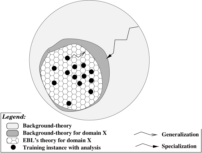
Figure 4: Two views of EBL: generalization and specialization

A most vivid summary of the difference between inductive learning and EBL is given in [Mitchell, 1997] page 334:“Purely inductive learning methods formulate general hypotheses by finding empirical regularities over the training examples. Purely analytical methods use prior knowledge to derive general hypotheses deductively”.

For specializing the background-theory, EBL resorts to analyzing the given explanations of the training instances. This analysis involves the extraction of the set of features (from the instance-representation which is a tuple of features) that is essential and sufficient for classifying each instance. For example, if the instance of a day contains features that do not influence the concept Rainy-day (e.g. year), then EBL’s conclusion is to “exclude” (i.e. mask) these features for this target concept. Besides this specialization step, EBL generalizes over the values that the features may take by computing for each explanation (proof tree) the weakest conditions under which the proof still holds. In other words, EBL transforms an explanation of many derivation-steps into a complex rule (also called macro-rule) which has the form: generalized-instance implies target-concept. The generalized-instance is the most general form of the instance, according to the background-theory, for which the explanation (proof) still holds.

Since EBL does not aim at learning a hypothesis in the absence of one, but rather to improve the performance of an existing background-theory, one often tends to underestimate EBL’s contribution. But consider for example the game of chess, which has a perfectly defined background-theory which consists of all rules of the game. It is clear that good chess players do not try all possibilities in their heads before they make a move. Instead, they develop some expertise through experience under the full awareness of the rules of the game. These good players seem to develop a more specialized and operational “theory” of chess that enables them to arrive faster at better results. EBL seems to provide part of the computational explanation of phenomena such as human learning from explanations for specialization and improving efficiency. Here it is worthwhile emphasizing that the term “efficiency” does not necessarily mean speed-up. Efficiency can mean an improvement in any aspect of a system’s performance such as time, space or overgeneration. There are no limitations in EBL that prevent employing it for improving any desired performance measure.

Finally, the EBL paradigm makes two major assumptions [Mitchell, 1997]: 1) the background-theory is correct (i.e. “sound”) and complete (i.e. has full coverage) with respect to the instance space and the target-concept at hand, 2) The training material does not contain any errors or inconsistencies. In cases where the background-theory is not perfect (i.e. incorrect and incomplete), Mitchell [Mitchell, 1997] suggests to combine EBL with inductive learning.

10.3.1 EBL: specification

The specification of the general scheme for an EBL algorithm consists of four preconditions and one postcondition. The preconditions are defined as follows:

Background theory:

A description language for the task at hand together with rules, assertions and facts about the task. For instance, in natural language parsing, the description languages used in the background-theories are usually grammars e.g. CFGs. Facts about the task are provided by a human annotator who is responsible for providing the right non-ambiguous descriptions.

Training examples:

A history of explicit explanations that are given by the background-theory to example instances of the concept being learned. In parsing, for example, this is a tree-bank annotated under a CFG, i.e. a derivation or a parse-tree constitutes an explanation for why a sequence of words is a sentence in the language of the (background theory) CFG.

Target concept:

A formal description, in terms of the alphabet of the background-theory, of the domain and the range of the function that is to-be-learned (this also defines the instance-scheme). For instance, when given a tree-bank annotated under a CFG $G$ = ($V_{N}$, $V_{T}$, $S$, ${\cal R}$), a target concept can be the notion of “constituency”; this concept is defined by $V^{+}$ as domain and by $V_{N}$$\cup\{NOT\}$ as range, where NOT denotes sequences that are not constituents. As an example, the instance-scheme could be in the form: XP($x_{1}\cdots x_{m}$), $m\geq~{}1$, expressing a CFG rule ${XP\rightarrow x_{1}\cdots x_{m}}$ (not necessarily a member in ${\cal R}$).

Operationality criterion:

A requirement on the form of the target concept (i.e. its domain and range), in order to render the learned hypothesis “operational” with respect to some measure. In parsing, this can be a formal requirement on any CFG rule that can be learned. For example, one could set an operationality criterion that limits the length of the right hand side of CFG rules, in order to limit the size of the CFG that is learned. Or, one could demand that the CFG rule be Right-Linear if one intends to parse using an FSM.

The postcondition is:

Postcondition:

To find a generalization of the instances of the target concept given in the training-examples, that satisfies the operationality criterion and the background theory. In our example on parsing, the generalization consists of CFG rules (or subtrees of the tree-bank trees, if one maintains also an internal structure for these rules) that satisfy the operationality criteria.

The operationality criteria represent in fact extra bias in order to render the learned knowledge, i.e. the target concept, operational. These are requirements on the form of the target-concept, which may originate in part from the background-theory and in part from knowledge of the “machinery”, which will be employed for exploiting the learned target-concept. For example, if one is planning to run the learned knowledge on a Finite-State Machine (FSM) then it is worth considering an operationality criterion stating that the target-concept must be a regular expression.

10.3.2 EBL: short literature overview

Historically speaking, EBL [DeJong, 1981, DeJong and Mooney, 1986, Mitchell et al., 1986] is the name of a unifying framework for various methods that learn from explanations of examples of a certain concept using a background-theory. In most existing literature, the main goal of EBL is faster recognition of concepts than the background-theory; EBL learns “shortcuts” in computation (called macro-operators or “chunks”), or directives for changing the thread of computation. EBL stores the learned macro-operators in the form of partial-explanations to previously seen input instances, in order to apply them in the future to “similar” input instances (in EBL, also “similarity” is assumed to be provided by the background-theory). However, as mentioned above, Speedup Learning is in fact only one area where EBL can be applied.

Past experience in Machine Learning cast doubt on the feasibility of improving performance by using EBL [Minton, 1990]. In his paper, Minton explains that EBL does not guarantee better performance, since the cost of applying the learned knowledge might outweigh the gain since EBL has no mechanism for measuring the utility of the learned knowledge. For this reason, Minton discusses a formula for computing the utility of knowledge during learning. Generally speaking, this formula is not part of EBL; it is an extension to the EBL scheme by e.g. statistical inference over large sets of training examples.

For an overview of the literature on EBL the reader is referred to chapter 4 of [Shavlik and Dietterich, 1990] and chapter 11 of [Mitchell, 1997]. For a formal framework and discussion of Speedup Learning the reader is referred to [Tadepalli and Natarajan, 1996]. For a study of the relation between EBL and partial-evaluation the reader is referred to [van Harmelen and Bundy, 1988].

11 Thesis goals and overview

The focus of this thesis is on the ambiguity problem in natural languages and their grammars. The primary goal is to present efficient solutions for the problem of ambiguity resolution in natural language parsing. The starting point for this study is that the solutions must be algorithmic and general, do not necessitate human intervention except for supplying the input, and are amenable to empirical assessment. The main vehicles that carry the present solutions are Machine Learning and Probability Theory.

As in various preceding work, the task of natural language parsing is conceptually divided in two modules: 1) the parser which is the module that generates the linguistic analyses that are associated with the input (i.e. the parse-space), and 2) the disambiguator which is the module that selects one preferred analysis from among the many that the parser generates. The parser is based on a grammar, e.g. a CFG or a TSG (not necessarily a competence grammar). The disambiguator is based on a probabilistic enrichment of the relations (e.g. subsentential-forms, partial-derivations, partial-trees) that can be expressed by the grammar of the parser. We refer to this probabilistic enrichment with the term probabilistic model. Despite of this conceptual devision of labour between both modules, it is easy to see that the parser also involves “disambiguation” because the grammar that underlies it already delimits the parse-space of the input even before probabilistic disambiguation starts. Therefore, the grammar itself constitutes another location where ambiguity resolution can take place.

For acquiring (or training) both the grammar and the probabilistic model, this work adopts the Corpus-Based view that it is most expedient to employ an unambiguously and correctly annotated (i.e. by a human) sample of real-life data as training material, i.e. a tree-bank. This offers the possibility that the resulting parser and disambiguator will answer to similar distributions as the sample that was used for training, which is considered representative of some domain of language use.

This thesis concentrates on the inefficiency aspect of existing performance models of ambiguity resolution. The thesis defends the hypothesis that the task of ambiguity resolution in parsing limited domains of language use can be implemented more efficiently and more accurately by integrating two complementary and interdependent disambiguation methods:

1. Through the automatic learning of a less ambiguous grammar from a tree-bank representing a specific domain. The main goal here is to cash in on the measurable biases in that domain (which are properties of human language processing in limited domains). We refer to this as off-line partial-disambiguation or grammar specialization through ambiguity reduction.

2. Through utilizing a probabilistic model that imposes a complete ordering on the space of analyses and allows the selection of a most probable analysis. This can be called on-line full-disambiguation. The DOP model is the most suitable candidate for this task since it generalizes over most existing probabilistic models of disambiguation.

These two manners of disambiguation are complementary: on-line disambiguation is applied only where it is impossible to disambiguate off-line without causing undergeneration. And they are interdependent since a less ambiguous grammar, acquired off-line, can serve as the linguistic annotation scheme for the tree-bank from which the probabilistic model is obtained.

Although on-line full disambiguation seems sufficient for ambiguity resolution, there are reasons to believe that off-line partial disambiguation by grammar specialization is an essential element of disambiguation:

• None of the existing probabilistic models has the property that frequently occurring and more grammatical input is processed faster. This is the main property accounted for by specialization by ambiguity reduction, i.e. off-line disambiguation as implemented in this thesis.

• A grammar that extremely overgenerates on some domain forms a bottleneck for any probabilistic model which is obtained from a tree-bank representing that domain and annotated under that grammar. Such an overgenerating grammar imposes an extreme strain on the probabilistic model: applying probabilistic computations that are based on a large table of probabilities to a large parse-space implies a very inefficient parser. This situation is most evident when parsing word-graphs output by a speech-recognizer using a DOP STSG as probabilistic model.

• When a performance model such as DOP employs a tree-bank that has an extremely overgenerating underlying grammar, it acquires a probabilistic grammar that has a large number of statistical parameters. It is common wisdom in probabilistic modeling that the larger the number of parameters, the more data are necessary for estimating them from relative frequencies. Therefore, large probabilistic grammars are more prone to sparse-data effects than smaller ones. Extreme overgeneration is a source of data-sparseness in probabilistic models.

Specialization by ambiguity-reduction provides solutions to these problems and combines very well with probabilistic models such as DOP.

The order of the subsequent chapters reflects the course of events that led to the shift in my subject of interest from parsing-algorithms to the more general subject of learning how to parse efficiently. After proving that some problems of probabilistic disambiguation are intractable (chapter 3) I arrived at the conclusion that it is necessary to develop non-traditional methods for improving the efficiency of parsing (chapter 4) and to combine them together with optimized (relatively) traditional methods (chapter 5). Next I elaborate on the contents of these chapters.

Chapters 3 and 5:

The choice for DOP for the task of on-line disambiguation implies a time- and space-bottleneck, because it employs huge probabilistic STSGs and involves complex computations. Chapters 3 and 5 study the computational aspects of disambiguation under the DOP model. Chapter 5 presents efficient parsing and disambiguation algorithms that provide useful solutions to some of the problems of disambiguation under DOP. The chapter presents optimized deterministic polynomial-time algorithms for computing the MPD (and the total probability) of a tree, a sentence, an FSM (word-graph without probabilities) and an SFSM (a word-graph as output by speech-recognizers). Moreover, it also suggests effective heuristics for the application of DOP, and exhibits extensive experiments with the DOP model on various domains and for various applications. These algorithms and heuristics have been fully implemented in the Data Oriented Parsing and DISambiguation environment (DOPDIS) [Sima’an, 1995].

In contrast to chapter 5, chapter 3 brings the (often negatively interpreted) news that some disambiguation problems under DOP are (currently and most probably in the future) not solvable in deterministic polynomial-time. It supplies a study of the computational complexity of (on-line) probabilistic disambiguation, under SCFGs and STSGs. It provides proofs that the following problems are NP-Complete: the problem of computing the MPP of a sentence or a word-graph under STSGs, the problem of computing the Most Probable Sentence (MPS) of a word-graph under STSGs and SCFGs. These proofs imply that it is highly unlikely that efficient deterministic polynomial-time solutions can be found. This redirects the research on finding solutions to these problems in non-conventional ways, e.g. off-line disambiguation as presented in chapter 4.

Chapter 4:

For off-line disambiguation, chapter 4 presents a brand new view on the subject of grammar specialization, embodied by the Ambiguity Reduction Specialization (ARS) framework. Rather than learn a grammar that has shorter derivations, as preceding work on grammar specialization expresses its goals, the ARS framework suggests to learn a less ambiguous grammar without jeopardizing coverage. Chapter 4 presents the ARS framework and derives from it two learning algorithms for grammar specialization. Grammar specialization under ARS improves the efficiency of parsing and disambiguation, especially on more frequent and longer input.

An interesting aspect of ARS is that it relates the following issues on parsing and disambiguation to each other: efficiency, partial-parsing, partial-disambiguation, and grammar and DOP specialization to specific domains. Grammar specialization in ARS is equal to reducing ambiguity only where possible (i.e. partial-disambiguation). The specialized-grammar in ARS is always partial to the original grammar (partial-parsing). Projecting a DOP STSG from the specialized tree-bank results in a specialized DOP model. Chapter 4 elaborates each of these issues.

A novel property of ARS is that it learns partial-parsers that can be combined with a full parser in a complementary manner; the full parser is engaged in the parsing processes only where and when necessary. The partial-parser can be implemented in various ways among which the most natural is a Cascade of Finite State Transducers. Chapter 4 discusses these issues of partial-parsing and full-parsing in detail.

Chapter 6:

The ARS learning and parsing algorithms are implemented in the Domain Ambiguity Reduction Specialization (DOARS) system. Chapter 6 discusses implementation issues of DOARS and exhibits an empirical study of the ARS algorithms on various domains. DOARS is evaluated on its own and in combination with DOPDIS on sentence and word-graph disambiguation.

Chapter 7:

Chapter 7 summarizes and discusses the general conclusions of this thesis.

Each of the subsequent chapters relies to some extent on the definitions and background information discussed in the present chapter. Nevertheless, to avoid a large background chapter, each chapter contains its own necessary definitions and background information. Therefore, reading the subsequent chapters can take place in any desired order.

Chapter 3 Complexity of Probabilistic Disambiguation

Probabilistic disambiguation, represented by the DOP model, constitutes one of the two methods of disambiguation that this thesis combines. A major question in applying probabilistic models is whether it is possible and how to transform optimization problems of probabilistic disambiguation to efficient algorithms ? The departure point in answering this question lies in classifying these problems according to the time-complexities of their solutions. A problem that does not have solutions of some desirable time-complexity, constitutes a source of inconvenience and demands special treatment.

The present chapter provides a proof that some of the common problems of probabilistic disambiguation, under DOP and similar models, belong to a class of problems for which we do not know whether we can devise deterministic polynomial-time algorithms. In fact, there is substantial evidence that the problems that belong to this class, the NP-complete class, do not have such algorithms. For NP-complete problems, the only known deterministic algorithms have exponential-time complexity. This is, to say the least, inconvenient since exponential-time algorithms imply a serious limitation on the kinds and sizes of applications for which probabilistic models can be applied.

For obvious reasons, the problems considered in this chapter are stated in a form that generalizes over the case of the DOP model. All these problems involve some form of probabilistic disambiguation under SCFG-based models [Jelinek et al., 1990, Black et al., 1993, Charniak, 1996] or STSG-based models [Sekine and Grishman, 1995, Bod, 1995a]. Moreover, the results of the present proofs apply also to TAG-based models [Schabes, 1992, Schabes and Waters, 1993, Resnik, 1992] and the proofs themselves have been adapted to prove that other similar problems of disambiguation are also NP-complete [Goodman, 1998]. The applications that face these hard disambiguation problems range from applications that involve parsing and interpretation of text to applications that involve speech-understanding and information retrieval.

12 Motivation

As mentioned earlier, an important facility of probabilistic disambiguation is that it enables the selection of a single analysis of the input. Parsing and disambiguation of some input, e.g. under the DOP model, can take place by maximizing the probability of some entity (in short “maximization-entity”). Chapter 5 exhibits efficient deterministic algorithms for some problems of disambiguation under DOP. Among these problems, there are the problems of computing the Most Probable Derivation (MPD) and computing the probability of an input tree/sentence/word-graph. These algorithms serve as useful disambiguation tools for various tasks and in various applications. However, there are many other applications for which the DOP model prescribes to compute other entities. For example, under current DOP, the disambiguation of sentences can (theoretically speaking) better take place by computing the Most Probable Parse (MPP). Another example is syntactic disambiguation in speech-understanding applications where the Most Probable Sentence (MPS) of a word-graph, produced by the speech-recognizer, is the desired entity.

In the present chapter we consider the problems of computing the MPP or the MPS for input sentences or word-graphs under STSGs in general. We provide proofs that these problems are NP-complete. This means that, as far as we know, there are no deterministic polynomial-time algorithms for computing these entities in an exact manner. For this reason, NP-complete problems are treated in practice as intractable problems. Surprisingly, the “intractability” of the problem of computing the MPS of a word-graph carries over to models that are based on SCFGs.

This work is not only driven by mathematical interest but also by the desire to develop efficient algorithms for these problems. As mentioned above, such algorithms can be useful for various applications that demand disambiguation facilities, e.g. speech-recognition and information retrieval. The proofs in this chapter serve us in various ways. They save us from investing time in searching for deterministic polynomial-time algorithms that do not exist. They provide an explanation for the source of complexity, an insight that can be useful in developing models that avoid the same intractability problems. They place our specific problems in a general class of problems, the NP-complete class, which has the property that if one of its members ever becomes solvable, due to unforseen research developments, in deterministic polynomial-time, all of its members will be solvable in deterministic polynomial-time and the algorithms will be directly available. And they form a license to redirect the research for solutions towards non-standard methods, discussed in the conclusions of this chapter.

The structure of this chapter is as follows. Section 13 provides a short overview of the theory of intractability, its notions, and its terminology. Section 14 states more formally the problems that this chapter deals with. Section 15 provides the proofs for each of the problems. Finally, section 16 discusses the conclusions of this study and the questions encountered that are still open.

13 Tractability and NP-completeness

This section provides a short overview of the notions of tractability and NP-completeness. The present discussion is not aimed at providing the reader with a complete account of the theory of NP-completeness. Rather, the aim is to provide the basic terminology and the references to the relevant literature. Readers that are interested in the details and formalizations of tractability and NP-completeness are referred to any of the existing text books on this subject e.g. [Garey and Johnson, 1981, Hopcroft and Ullman, 1979, Lewis and Papadimitriou, 1981, Davis and Weyuker, 1983, Barton et al., 1987].

The present discussion is formal only where that is necessary. It employs the terminology which is common in text books on the subject e.g. [Garey and Johnson, 1981]. For a formalization of this terminology and a discussion of the limitations of this formalization, the reader is referred to chapters 1 and 2 of [Garey and Johnson, 1981].

Decision problems:

The point of focus of this section is the notion of a tractable decision problem. Informally speaking, a problem is a pair: a generic instance, stating the formal devices and components involved in the problem, and a question asked in terms of the generic instance. A decision problem is a problem where the question can have only one of two possible answers: Yes or No. For example, the well known 3SAT (3-satisfiability) problem is stated as follows:

INSTANCE: A Boolean formula in 3-conjunctive normal form (3CNF) over the variables $u_{1},\ldots,u_{n}$. We denote this generic instance of 3SAT with the name INS. Moreover, we denote the formula of INS by the generic form:

$$(d_{11}\vee d_{12}\vee d_{13})\wedge(d_{21}\vee d_{22}\vee d_{23})\wedge\cdots\wedge(d_{m1}\vee d_{m2}\vee d_{m3})$$

where $m\geq 1$ and $d_{ij}$ is a literal over {$u_{1},\ldots,u_{n}$}, for all $1\leq~{}i~{}\leq~{}m$ and all $1\leq~{}j~{}\leq~{}3$. This formula will also be denoted $C_{1}\wedge C_{2}\wedge\cdots\wedge C_{m}$, where $C_{i}$ represents $(d_{i1}\vee~{}d_{i2}\vee~{}d_{i3})$, for all $1\leq~{}i~{}\leq~{}m$.

QUESTION: Is the formula in INS satisfiable ? i.e. is there an assignment of values true or false to the Boolean variables $u_{1},\ldots,u_{n}$ such that the given formula is true ?

Decision problems are particularly convenient for complexity studies mainly because of the natural correspondence between them and the formal object called “language” (usually languages and questions in terms of set-membership are the formal forms of decision problems). The size or length of an instance of a decision problem is the main variable in any measure of the time-complexity of the algorithmic solutions to the problem (in case these exist). Roughly speaking, this length is measured with respect to some reasonable encoding (deterministic polynomial-time computable) from each instance of the decision problem to a string in the corresponding language. In order not to complicate the discussion more than necessary, we follow common practice, as explained in [Garey and Johnson, 1981], and assume measures of length that are more “natural” to the decision problem at hand (knowing that it is at most a polynomial-time cost to transform an instance to a string in the language corresponding to the decision problem). For 3SAT, for example, the length of an instance is $3m+(m-1)+2m$, i.e. the number of symbols in the formula is linear in the number of conjuncts $m$.

Tractable problems and class P:

While Computability Theory deals with the question whether a given problem has an algorithmic solution or not, the theory of NP-completeness deals, roughly speaking, with the question whether the problem has a general solution that is computationaly attainable in practice. In other words:

Is there a (deterministic) algorithmic solution, which computes the answer to every instance of the problem and for every input to that instance, of length $n\geq 1$, in a number of computation steps that is proportional to a “cheap” function in $n$ ?

The problem with defining the term “cheap” lies in finding a borderline between those functions that can be considered expensive and those that can be considered cheap. A first borderline that has been drawn by a widely accepted thesis (Cook-Karp) is between polynomials and exponentials. Problems for which there is a deterministic polynomial-time solution are called tractable. Other problems for which there are only deterministic exponential-time solutions are called intractable.

The main motivation behind the Cook-Karp descrimination between polynomials and exponentials is the difference in rate of growth between these two families. Generally speaking, exponentials tend to grow much faster than polynomials. Strong support for the Cook-Karp thesis came from practice: most practically feasible (“naturally occuring”) problems (in computer science and natural language processing) have deterministic polynomial-time solutions where the polynomial is of low degree. Only very few problems with exponential-time solutions are feasible in practice; usually these problems have a small expected input length. Moreover, the overwhelming majority of problems that are not solvable in deterministic polynomial-time turn out to be not feasible in practice. For further discussions on the stability of this thesis (also in the face of massively parallel computers) the reader is reffered to the text books listed above, especially [Garey and Johnson, 1981, Barton et al., 1987].

Class P and class NP-hard:

As stated above, according to the Cook-Karp thesis, a decision problem (i.e. every one of its instances) that has a deterministic polynomial-time solution in the length of its input is considered tractable. All other decision problems are considered intractable. The tractable decision problems, i.e. those that have a polynomial-time deterministic algorithmic solution (a so called Deterministic Turing Machine (DTM)), are referred to with the term class P problems. All other problems, that are intractable, are referred to with the term NP-hard problems (see below for the reason for this terminology).

Class NP:

Interestingly, there exist problems that are solvable in polynomial-time provided that the algorithmic solution has access to an oracle, which is able to guess the right computation-steps without extra cost (a so called Non-deterministic Turing Machine (NDTM)). Note that every problem in class P is found among these so called Non-deterministic Polynomial-time solvable problems, also called class NP problems (i.e. P $\subseteq$ NP). The question is, of course, are there more problems in class NP than in class P ? This is where we enter the gray zone in the theory of NP-completeness: nobody yet knows the answer to this question. Most computer scientists suspect, however, that P $\neq$ NP.

NP-complete problems:

Strong evidence to the hypothesis P $\neq$ NP is embodied by the discovery of many practical and theoretical problems that are known to be in class NP but for which nobody yet knows how to devise deterministic polynomial-time solutions; these problems are in class NP but are not known to be in class P. In fact, if P$\neq$NP is true then these problems are indeed NP-hard (and also in NP). This set of problems is called the class of NP-complete problems. Thus, NP-complete problems are those that lie in the difference between class P and class NP, if indeed P$\neq$NP is true.

Now, the term NP-hard can be explained as denoting those problems that are at least as hard as any problem that is in NP (the formal definition of this relies on the notion of deterministic polynomial-time reducibility, which we discuss below). And the NP-complete problems are the hardest among all problems that are in NP.

Proving NP-completeness:

To prove that a given problem $L$ is NP-hard, it is sufficient to show that another problem that is known to be NP-complete is polynomial-time reducible to $L$. This is done by providing a polynomial-time reduction (i.e. function) from the NP-complete problem to problem $L$. Such a reduction shows how every instance of the NP-complete problem can be transformed into an instance of problem $L$. Naturally, the reduction must be answer-preserving, i.e. for every instance of the NP-complete problem and for every possible input, the instance answers Yes to that input iff the $L$-instance (resulting from the reduction) also does answer Yes to the transformed-form of that input. Note that the reducibility relation between problems is a transitive relation.

Thus, once we lay our hands on one NP-complete problem, we can prove other problems to be NP-hard. Fortunately, a problem that has been proven to be NP-complete is the 3SAT problem stated above. Therefore 3SAT can serve us in proving other problems to be NP-hard. In addition, proving that a problem is NP-hard and that it is also in NP, proves it to be NP-complete.

The NP-complete “club”:

Note that all NP-complete problem are polynomial-time reducible to each other. This makes the NP-complete problems an interesting class of problems: either all of them can be solved in deterministic polynomial-time or none will ever be. Discovering one NP-complete problem that has a deterministic polynomial-time solution also implies that P = NP.

Currently there are very many problems that are known to be NP-complete, but none has been solvable in deterministic polynomial-time yet. The efforts put into the study of these problems in order to solve them in deterministic polynomial-time have been immense but without success. This is the main evidence strengthening the hypothesis that P$\neq$NP and that NP-complete problems are also intractable. In the current situation, where we don’t know how to (and whether we can) solve NP-complete problems in deterministic polynomial-time, we are left with a fact: all current solutions to these problems (in general) are not feasible, i.e. these problems are “practically intractable”. This might change in the future, but such change seems highly unlikely to happen soon. In any event, the main motivation behind proving that a new problem is NP-complete lies in saving the time spent on searching for a deterministic polynomial-time solution that most likely does not exist. Of course, proving a problem to be NP-complete does not imply that the problem should be put on the shelf. Rather, it really provides a motivation to redirect the effort towards other kinds of feasible approximations to that problem.

Optimization problems and NP-completeness:

In this work the focus is on optimization problems rather than decision problems. In general, it is possible to derive from every optimization problem a decision problem that is (at most) as hard as the optimization problem [Garey and Johnson, 1981]. Therefore, it is possible to prove NP-completeness of optimization problems through proving the NP-completeness of the decision problems derived from them. To derive a suitable decision problem from a given maximization/minimization problem, the QUESTION part of the maximization/minimization problem is stated differently: rather than asking for the maximum/minimum, the question asks whether there is a value that is larger/smaller than some lower/upper bound that is supplied as an additional parameter to the problem. For example, the problem of computing the maximum probability of a sentence of the intersection between an SCFG and an FSM, is transformed to the problem of deciding whether the intersection between an SCFG and an FSM contains a sentence of probability that is at least equal to $p$, where $0<p\leq 1$ is an extra input to the decision problem that serves as a “threshold”.

14 Problems in probabilistic disambiguation

To start, the generic devices that are involved in the problems, which this chapter deals with, are SCFGs, STSGs and word-graphs (SFSMs and FSMs). For word-graphs (SFSMs and FSMs), it is more convenient to consider a special case, which we refer to with the term “sequential word-graphs”, defined as follows:

Sequential word-graph (SWG):

A sequential word-graph over the alphabet $Q$ is$Q_{1}\times\cdots\times Q_{m}$, where $Q_{i}\subseteq Q$, for all $1\leq~{}i\leq~{}m$. We denote a sequential word-graph with $Q^{m}$ if $Q_{i}~{}=~{}Q$, for all $1\leq~{}i\leq~{}m$.

Note that this defines a sequential word-graph in terms of cartesian products of sets of the labels on the transitions (every $Q_{i}$ is such a set); transforming this notation into an FSM is rather easy to do ($Q$ is the set of transitions where the set of states is simply $\{0,\cdots,m+1\}$ and all transitions are between states $i$ and $i+1$, state $0$ is the start state and state $m+1$ is the final state). In the sequel, we refer to an SWG with the more general term word-graph. This need not entail any confusion, this chapter refers to SWGs only, and any statement in the proofs that applies to SWGs automatically applies to word-graphs in general.

14.1 The optimization problems

Now it is time to state the optimization problems that this study concerns. Subsequently, these problems are transformed into suitable decision problems that will be proven to be NP-complete in section 15.

The first problem which we discuss concerns computing the Most Probable Parse of an input sentence under an STSG. This problem was put forward in [Bod, 1993a] and was discussed later on in [Sima’an et al., 1994, Bod, 1995b, Sima’an, 1997b]. These earlier efforts tried to supply algorithmic solutions to the problem: none of the solutions turned out to be deterministic polynomial-time. Then came the proof of NP-completeness [Sima’an, 1996], which forms the basis for the proof given in this chapter. The problem MPP is stated as follows:

1. Problem MPP:

   INSTANCE:

   An STSG $G$ and a sentence $w_{0}^{n}$.

   QUESTION:

   What is the MPP of sentence $w_{0}^{n}$ under STSG $G$ ?

The role of the MPP in the world of applications is rather clear: in order to derive the semantics of an input sentence, most Natural Language Processing systems (and the linguistic theories they are based on) assume that one needs a syntactic representation of that sentence. Under some linguistic theories, the syntactic representation is a parse-tree. DOP and many other probabilistic models select the MPP as the parse that most probably reflects the right syntactic structure of the input sentence. Applications in which problem MPP is encountered include many systems for parsing and interpretation of text.

A related problem is the problem of computing the MPP for an input word-graph, rather than a sentence, under an STSG:

1. Problem MPPWG:

   INSTANCE:

   An STSG $G$ and a sequential word-graph $SWG$.

   QUESTION:

   What is the MPP of $SWG$ under STSG $G$ ?

Applications of this problem are similar to the applications of problem MPP. In these applications, the input sentence is not a priori known and the parser must select the most probable of the set of parses of all sentences which the word-graph accepts. By selecting the MPP, the parser selects a sentence of the word-graph also. Typical applications lie in Speech Understanding, morphological analysis, but also in parsing sequences of words after PoS-tagging by a tagger that provides at least one (rather than exactly one) PoS-tag per word (packed in a word-graph).

The third problem is the following:

1. Problem MPS:

   INSTANCE:

   An STSG $G$ and a sequential word-graph $SWG$.

   QUESTION:

   What is the Most Probable Sentence (MPS) in $SWG$ under STSG $G$ ?

This problem has applications that are similar to problem MPPWG. In Speech Understanding it is often argued that the language model should select the MPS rather than the MPP of the input word-graph. Selecting the MPS, however, does not entail the selection of a syntactic structure for the sentence, a necessity for interpretation of the spoken utterance.

And finally:

1. Problem MPS-SCFG:

   INSTANCE:

   An SCFG $G$ and a sequential word-graph $SWG$.

   QUESTION:

   What is the MPS in $SWG$ under SCFG $G$ ?

This problem is equal to a special case of problem MPS: an SCFG is equal to an STSG in which the maximum depth of subtrees is limited to 1 (see section 27). Applications that face this problem are similar to those that face problem MPS described above.

14.2 The corresponding decision problems

The decision problems that correspond to problems MPP, MPPWG, MPS and MPS-SCFG are given the same names:

1. Decision problem MPP:

   INSTANCE:

   An STSG $G$, a sentence $w_{0}^{n}$ and a real number $0<p\leq 1$.

   QUESTION:

   Does STSG $G$ generate for sentence $w_{0}^{n}$ a parse for which it assigns a probability greater or equal to $p$ ?

1. Decision problem MPPWG:

   INSTANCE:

   An STSG $G$, a sequential word-graph $SWG$ and a real number $0<p\leq 1$.

   QUESTION:

   Does STSG $G$ generate for $SWG$ a parse for which it assigns a probability greater or equal to $p$ ?

1. Decision problem MPS:

   INSTANCE:

   An STSG $G$, a sequential word-graph $SWG$ and a real number $0<p\leq 1$.

   QUESTION:

   Does $SWG$ accept a sentence for which STSG $G$ assigns a probability greater or equal to $p$ ?

1. Decision problem MPS-SCFG:

   INSTANCE:

   An SCFG $G$, a sequential word-graph $SWG$ and a real number $0<p\leq 1$.

   QUESTION:

   Does $SWG$ accept a sentence for which SCFG $G$ assigns a probability greater or equal to $p$ ?

In the sequel we refer to the real value $p$ in these decision problems with the terms “threshold” and “lower bound”.

Figure 5: The elementary-trees for the example 3SAT instance

15 NP-completeness proofs

As section 13 explains, for proving the NP-completeness of some problem it is necessary to prove that the problem is NP-hard and is a member of class NP. For proving NP-hardness, it is necessary to exhibit a suitable reduction from every instance of 3SAT to every instance of the problem at hand. This is what we do next for each of the decision problems listed in the preceding section. To this end, we restate the generic instance INS of 3SAT here:

INSTANCE: A Boolean formula in 3-conjunctive normal form (3CNF) over the variables $u_{1},\ldots,u_{n}$:

$$(d_{11}\vee d_{12}\vee d_{13})\wedge(d_{21}\vee d_{22}\vee d_{23})\wedge\cdots\wedge(d_{m1}\vee d_{m2}\vee d_{m3})$$

where $m\geq 1$ and $d_{ij}$ is a literal over {$u_{1},\ldots,u_{n}$}, for all $1\leq~{}i~{}\leq~{}m$ and all $1\leq~{}j~{}\leq~{}3$. This formula is also denoted $C_{1}\wedge C_{2}\wedge\cdots\wedge C_{m}$, where $C_{i}$ represents $(d_{i1}\vee~{}d_{i2}\vee~{}d_{i3})$, for all $1\leq~{}i~{}\leq~{}m$.

QUESTION: Is the formula in INS satisfiable ?

Proposition 3.1

Decision problems MPP, MPPWG, MPS and MPS-SCFG are NP-complete.

15.1 A guide to the reductions

The reductions in the next section are structured as follows. The first reduction is conducted from 3SAT to MPPWG and from 3SAT to MPS simultaneously, i.e. the same reduction serves proving both problems to be NP-hard. Then the reductions from 3SAT to MPP and from 3SAT to MPS-SCFG are obtained from the preceding reduction by some minor changes.

15.2 3SAT to MPPWG and MPS simultaneously

In the following, a reduction is devised which proves that both MPPWG and MPS are NP-hard. For convenience, the discussion concentrates on problem MPPWG, but also explains why the same reduction is suitable also for MPS.

The reduction from the 3SAT instance INS to an MPPWG instance must construct an STSG, a word-graph and a threshold value in deterministic polynomial-time. Moreover, the answers to the MPPWG instance must correspond exactly to the answers to INS. The presentation of the reduction shall be accompanied by an example of the following 3SAT instance [Barton et al., 1987]:

$$(u_{1}\vee\overline{u}_{2}\vee u_{3})\wedge(\overline{u}_{1}\vee u_{2}\vee\overline{u}_{3}),$$

where $u_{1}$, $u_{2}$ and $u_{3}$ are Boolean variables.

Note that a 3SAT instance is satisfiable iff at least one of the literals in each conjunct is assigned the value true. Implicit in this, but crucial, the different occurrences of the literals of the same variable must be assigned values consistently. These two observations constitute the basis of the reduction. The reduction must capture these two “satisfiability-requirements” of INS in the problem-instances that it constructs. For example, for MPPWG, we will construct an STSG and a WG. The WG will be $WG~{}=~{}\{{\bf T},~{}{\bf F}\}^{{\bf 3m}}$, where $3m$ is the number of literals in the formula of INS. The STSG will be constructed such that it has two kinds of derivations for every path in WG that constitutes a solution for INS (if there is such a solution): one kind of derivations takes care of the consistent assignment of truth values, and the other takes care of assigning the value true for exactly one literal in every conjunct. The derivations will have such probabilities that will enable us to know whether a path in WG is a solution for INS by inspecting the probability of that path; the probability of a path in WG will tell us whether the STSG derives that path by enough derivations of each kind in order for that path to be a solution for INS.

15.2.1 The reduction:

The reduction constructs an STSG and a word-graph. The STSG has start-symbol labeled $S$, two terminals represented by T and F , non-terminals which include (beside $S$) all $C_{k}$, for $1\leq k\leq m$, and both literals of each Boolean variable of the formula of INS. The set of elementary-trees and probability function and the word-graph are constructed as follows:

1. The reduction constructs for each Boolean variable $u_{i}$, $1\leq~{}i~{}\leq~{}n$, two elementary-trees that correspond to assigning the values true and false to $u_{i}$ consistently through the whole formula. Each of these elementary-trees has root $S$, with children $C_{k}$, $1\leq~{}k~{}\leq~{}m$, in the same order as they appear in the formula of INS; subsequently the children of $C_{k}$ are the non-terminals that correspond to its three disjuncts $d_{k1}$,  $d_{k2}$ and $d_{k3}$. And finally, the assignment of true (false) to $u_{i}$ is modeled by creating a child terminal T (resp. F ) to each non-terminal $u_{i}$ and F (resp. T ) to each $\overline{u}_{i}$. The two elementary-trees for $u_{1}$, of our example, are shown in the top left corner of figure 5.

2. The reduction constructs three elementary-trees for each conjunct $C_{k}$. The three elementary-trees for conjunct $C_{k}$ have the same internal structure: root $C_{k}$, with three children that correspond to the disjuncts $d_{k1}$,  $d_{k2}$ and $d_{k3}$. In each of these elementary-trees exactly one of the disjuncts has as a child the terminal T ; in each of them this is a different one. Each of these elementary-trees corresponds to the conjunct where one of the three possible literals is assigned the value T . For the elementary-trees of our example see the top right corner of figure 5.

3. The reduction constructs for each of the literals of each variable $u_{i}$ two elementary-trees where the literal is assigned in one case T and in the other F . Figure 5 shows these elementary-trees for variable $u_{1}$ in the bottom left corner.

4. The reduction constructs one elementary-tree that has root $S$ with children $C_{k}$, $1\leq~{}k~{}\leq~{}m$, in the same order as these appear in the formula of INS (see the bottom right corner of figure 5).

5. The reduction assigns probabilities to the elementary-trees that were constructed by the preceding steps. The probabilities of the elementary-trees that have the same root non-terminal must sum up to $1$. The probability of an elementary-tree with root $S$ that was constructed in step 1 of this reduction is a value $p_{i}$, $1\leq~{}i\leq~{}n$, where $u_{i}$ is the only variable of which the literals in the elementary-tree at hand are lexicalized (i.e. have terminal children). Let $n_{i}$ denote the number of occurrences of both literals of variable $u_{i}$ in the formula of INS. Then $p_{i}$ = $\theta~{}(\frac{1}{2})^{n_{i}}$, for some real $\theta$ that has to fulfill some conditions which will be derived next. The probability of the tree rooted with $S$ and constructed at step 4 of this reduction must then be $p_{0}~{}=~{}[1~{}-~{}2\sum_{i=1}^{n}p_{i}]$. The probability of the elementary-trees of root $C_{k}$ (step 2) is $(\frac{1}{3})$, and of root $u_{i}$ or $\overline{u}_{i}$ (step 3) is $(\frac{1}{2})$. For our example some suitable probabilities are shown in figure 5.

Let $Q$ denote a threshold probability that shall be derived below. The MPPWG (MPS) instance produced by this reduction is:

INSTANCE:

The STSG produced by the above reduction (probabilities are derived below), the word-graph $WG~{}=~{}\{{\bf T},~{}{\bf F}\}^{{\bf 3m}}$, and a probability value $Q$ (also derived below).

QUESTION:

Does this STSG generate for the word-graph $WG=\{{\bf T},~{}{\bf F}\}^{{\bf 3m}}$ a parse (resp. a sentence) for which it assigns a probability greater than or equal to $Q$ ?

Deriving the probabilities and the threshold:

The parses generated by the constructed STSG differ only in the sentences on their frontiers. Therefore, if a sentence is generated by this STSG then it has exactly one parse. This justifies the choice to reduce 3SAT to MPPWG and MPS simultaneously.

By inspecting the STSG resulting from the reduction, one can recognize two types of derivations in this STSG:

1. The first type corresponds to substituting for a substitution-site (i.e literal) of any of the $2n$ elementary-trees constructed in step 1 of the reduction. This type of derivation corresponds to assigning values to all literals of some variable $u_{i}$ in a consistent manner. For all $1\leq i\leq n$ the probability of a derivation of this type is

   $$p_{i}(\frac{1}{2})^{3m-n_{i}}~{}=~{}\theta(\frac{1}{2})^{3m}$$

2. The second type of derivation corresponds to substituting the elementary-trees that $C_{k}$ as root in $S$ $\rightarrow$ $C_{1}\ldots~{}C_{m}$, and subsequently substituting in the substitution-sites that correspond to literals. This type of derivation corresponds to assigning to at least one literal in each conjunct the value true. The probability of any such derivation is

   $$p_{0}(\frac{1}{2})^{2m}(\frac{1}{3})^{m}~{}=~{}[1-2\theta\sum_{i=1}^{n}(\frac{1}{2})^{n_{i}}](\frac{1}{2})^{2m}(\frac{1}{3})^{m}$$

Now we derive both the threshold $Q$ and the parameter $\theta$. Any parse (or sentence) that fulfills both the “consistency of assignment” requirements and the requirement that each conjunct has at least one literal with child T , must be generated by $n$ derivations of the first type and at least one derivation of the second type. Note that a parse can never be generated by more than $n$ derivations of the first type. Thus the threshold $Q$ must be set at:

$$Q=n\theta(\frac{1}{2})^{3m}~{}+~{}[1-2\theta\sum_{i=1}^{n}(\frac{1}{2})^{n_{i}}](\frac{1}{2})^{2m}(\frac{1}{3})^{m}$$

However, $\theta$ must fulfill some requirements for our reduction to be acceptable:

1. For all i: $0<p_{i}<1$. This means that for $1\leq~{}i\leq~{}n$: $0~{}<~{}\theta(\frac{1}{2})^{n_{i}}~{}<~{}1$, and $0<p_{0}<1$. However, the last requirement on $p_{0}$ implies that

   $$0~{}<~{}2\theta\sum_{i=1}^{n}(\frac{1}{2})^{n_{i}}~{}<~{}1,$$

   which is a stronger requirement than the other $n$ requirements. This requirement can also be stated as follows: $0<\theta<\frac{1}{2\sum_{i=1}^{n}(\frac{1}{2})^{n_{i}}}$.

2. Since we want to be able to know whether a parse is generated by a second type derivation only by looking at the probability of the parse, the probability of a second type derivation must be distinguishable from first type derivations. Moreover, if a parse is generated by more than one derivation of the second type, we do not want the sum of the probabilities of these derivations to be mistaken for one (or more) first type derivation(s). For any parse, there are at most $3^{m}$ second type derivations (e.g. the sentence T $\dots$T ). Therefore we require that:

   $$3^{m}[1-2\theta\sum_{i=1}^{n}(\frac{1}{2})^{n_{i}}](\frac{1}{2})^{2m}(\frac{1}{3})^{m}~{}<~{}\theta(\frac{1}{2})^{3m}$$

   Which is equal to demanding that: $\theta~{}>~{}\frac{1}{2\sum_{i=1}^{n}(\frac{1}{2})^{n_{i}}~{}+~{}(\frac{1}{2})^{m}}$.

3. For the resulting STSG to be a probabilistic model, the “probabilities” of parses and sentences must be in the interval $(0,1]$. This is taken care of by demanding that the sum of the probabilities of elementary-trees that have the same root non-terminal is 1, and by the definition of the derivation’s probability, the parse’s probability, and the sentence’s probability.

Existence of $\theta$:

There exists a $\theta$ that fulfills all these requirements because the lower bound $\frac{1}{2\sum_{i=1}^{n}(\frac{1}{2})^{n_{i}}~{}+~{}(\frac{1}{2})^{m}}$ is always larger than zero and is strictly smaller than the upper bound  $\frac{1}{2\sum_{i=1}^{n}(\frac{1}{2})^{n_{i}}}$.

Polynomiality of the reduction:

This reduction is deterministic polynomial-time in $m$ and $n$ (note that $n\leq 3m$ always). It constructs not more than $2n+1+3m+4n$ elementary-trees, each consisting of at most $7m+1$ nodes. And the computation of the probabilities and the threshold is also conducted in deterministic polynomial-time.

The reduction preserves answers:

The proof that this reduction preserves answers concerns the two possible answers Yes and No:

1. If INS’s answer is Yes then there is an assignment to the variables that is consistent and where each conjunct has at least one literal assigned true. Any possible assignment is represented by one sentence in $WG$. A sentence which corresponds to a “successful” assignment must be generated by $n$ derivations of the first type and at least one derivation of the second type; this is because the sentence $w_{1}^{3m}$ fulfills $n$ consistency requirements (one per Boolean variable) and has at least one T as $w_{3k+1}$, $w_{3k+2}$ or $w_{3k+3}$, for all $0\leq~{}k~{}<~{}m$. Both this sentence and its corresponding parse have probability $\geq~{}Q$. Thus MPPWG and MPS also answer Yes.

2. If INS’s answer is No, then all possible assignments are either not consistent or result in at least one conjunct with three false disjuncts, or both. The sentences (parses) that correspond to non-consistent assignments each have a probability that cannot result in a Yes answer. This is the case because such sentences have fewer than $n$ derivations of the first type, and the derivations of the second type can never compensate for that (the requirements on $\theta$ take care of this). For the sentences (parses) that correspond to consistent assignments, there is at least some $0\leq~{}k~{}<m$ such that $w_{3k+1}$, $w_{3k+2}$ and $w_{3k+3}$ are all F . These sentences do not have second type derivations. Thus, there is no sentence (parse) that has a probability that can result in a Yes answer; the answer of MPPWG and MPS is NO   $\Box$

To summarize, we have deterministic polynomial-time reductions, that preserve answers, from 3SAT to MPPWG and from 3SAT to MPS. We conclude that MPPWG and MPS are both NP-hard problems. Now we prove NP-completeness in order to show that these problems are deterministic polynomial-time solvable iff P = NP.

15.2.2 NP-completeness of MPS and MPPWG

Now we show that MPPWG and MPS are in NP. A problem is in NP if it is decidable by a non-deterministic Turing Machine in polynomial-time. In general, however, it is possible to be less formal than this. It is sufficient to exhibit a suitable non-deterministic algorithm, which does the following: it proposes some entity as a solution (e.g. a parse for MPPWG and a sentence for MPS), and then computes an answer (Yes/NO) to the question of the decision problem, on this entity, in deterministic polynomial-time (cf. [Garey and Johnson, 1981, Barton et al., 1987]). The non-deterministic part lies in guessing or proposing an entity as a solution.

For MPPWG, a possible algorithm proposes a parse, from the set of all parses which the STSG $G$ assigns to $WG$, and computes its probability in deterministic polynomial-time, using the algorithms of chapter 5, and verifies whether this probability is larger or equal to the threshold $p$. Similarly, an algorithm for MPS proposes a sentence, from those accepted by the word-graph, and computes its probability in polynomial-time, using the algorithms in chapter 5, and then verifies whether this probability is larger or equal to the threshold $p$. In total, both algorithms are non-deterministic polynomial-time, a thing that proves that MPPWG and MPS are both in class NP.

In summary, now we proved that decision problems MPPWG and MPS are both NP-hard and in NP, therefore both are NP-complete problems. Therefore, the corresponding optimization problems MPPWG and MPS are NP-hard.

15.3 NP-completeness of MPP

The NP-completeness of MPP can be easily deduced from the proof in section 15.2. The proof of NP-hardness of MPP is based on a reduction from 3SAT to MPP obtained from the preceding reduction by minor changes. The main idea now is to construct a sentence and a threshold, and to adapt the STSG in such a way, that the sentence has many parses, each corresponding to some possible assignment of truth values to the literals of the 3SAT instance. As in the preceding reduction, the STSG will have at most two kinds of derivations and suitable probabilities; again the probabilities of the two kinds of derivations enable inspecting whether a parse is generated by enough derivations that it corresponds to an assignment that satisfies the 3SAT instance, i.e. a consistent assignment that assigns the value true to at least one literal in every conjunct.

The preceding reduction is adapted as follows. In the reduction, the terminals of the constructed STSG are now fresh new symbols $v_{ij}$, $1\leq~{}i~{}\leq~{}m$ and $1\leq~{}j~{}\leq~{}3$, instead of T and F ; the symbols T and F become non-terminals in the STSG of the present reduction. Then, some of the elementary-trees and some of the probabilities, constructed by the preceding reduction, are adapted as follows (any entity not mentioned below remains the same):

1. In each elementary-tree, constructed in step 1 or step 2 of the preceding reduction (with root node labeled either $S$ or $C_{k}$), the leaf node labeled T /F , which is the child of the $j$th child (a literal) of $C_{k}$, now has a child labeled $v_{kj}$.

2. Instead of each of the elementary-trees with a root labeled with a literal (i.e. $u_{k}$ or $\overline{u}_{k}$), constructed in step 3 of the preceding reduction, there are now $3m$ elementary-trees, each corresponding to adding a terminal-child $v_{ij}$, $1\leq~{}i~{}\leq~{}m$ and $1\leq~{}j~{}\leq~{}3$, under the (previously leaf) node labeled T /F .

3. The probability of an elementary-tree rooted by a literal (adapted in the preceding step) is now $\frac{1}{6m}$.

4. The probabilities of elementary-trees rooted with $C_{k}$ do not change.

5. The probabilities of the elementary-trees that has a root labeled $S$ are adapted from the previous reduction by substituting for every $(\frac{1}{2})$ the value $\frac{1}{6m}$.

6. The threshold $Q$ and the requirements on $\theta$ are also updated accordingly, and then derived as done in the preceding reduction.

7. The sentence, which the reduction constructs, is $v_{11}\ldots~{}v_{m3}$.

8. And the decision problem’s question is whether there is a parse generated by the newly constructed STSG for sentence $v_{11}\ldots~{}v_{m3}$, that has probability larger than or equal to $Q$ ?

The proofs that this reduction is polynomial-time and answer-preserving are very similar to that in section 15.2. It is easy also to prove that MPP is in class NP (very much similarly to MPPWG). Therefore, the decision problem MPP is NP-complete.

15.4 NP-completeness of MPS-SCFG

The decision problem MPS is NP-complete also under SCFG, i.e. MPS-SCFG is NP-complete. The proof is easily deducible from the proof concerning MPS for STSGs. The reduction is a simple adaptation of the reduction for MPS. Every elementary-tree of the MPS reduction is now simplified by “masking” its internal structure, thereby obtaining simple CFG productions. Crucially, each elementary-tree results in one unique CFG production. The probabilities are kept the same and also the threshold. The word-graph is also the same word-graph as in the reduction of MPS. The present decision-problem’s question is: does the thus created SCFG generate a sentence with probability $\geq~{}Q$, accepted by the word-graph $WG~{}=~{}\{{\bf T},~{}{\bf F}\}^{{\bf 3m}}$.

Note that for each derivation, which is possible in the STSG of problem MPS there is one corresponding unique derivation in the SCFG of problem MPS-SCFG. Moreover, there are no extra derivations. Of course, each derivation in the SCFG of problem MPS-SCFG generates a different parse. But that does not affect the probability of a sentence at all: it remains the sum of the probabilities of all derivations that generate it in the SCFG. The rest of the proof follows directly from section 15.2. Therefore, computing the MPS of a word-graph for SCFGs is also NP-complete.

16 Conclusions and open questions

We conclude that optimization problems MPP, MPPWG and MPS are NP-complete. This implies that computing the maximization entities involved in these problems (respectively MPP of a sentence, MPP of a word-graph and MPS of a word-graph) under STSG- and STAG-based models is (as far as we know) not possible in deterministic polynomial-time; examples of such models are respectively [Sekine and Grishman, 1995, Bod, 1995a] and [Schabes, 1992, Schabes and Waters, 1993, Resnik, 1992]. In addition, we conclude that problem MPS-SCFG is also NP-complete; note that MPS-SCFG concerns SCFGs, i.e. the “shallowest” of all STSGs. This is, to say the least, a serious inconvenience for applying probabilistic models to Speech-Understanding and other similar applications. In particular, the models that compute probabilities in the same manner as DOP does, clearly suffer from this inconvenience, e.g. SCFG-based models [Jelinek et al., 1990, Black et al., 1993, Charniak, 1996], STSG-based models [Sekine and Grishman, 1995, Bod, 1995a], and TAG-based models [Schabes, 1992, Schabes and Waters, 1993, Resnik, 1992].

The proof in this chapter helps to understand why these problems are so hard to solve efficiently. The fact that computing the MPS of a word-graph under SCFGs is also NP-complete implies that the complexity of these problems is not due to the kind of grammar underlying the models. Rather, the main source of NP-completeness is the following common structure of these problems:

Each of these problems searches for an entity that maximizes the sum of the probabilities of processes that are defined in terms of that entity.

For example, in problem MPS-SCFG, one searches for the sentence, which maximizes the sum of the probabilities of the derivations that generate that sentence; to achieve this, it is necessary to maintain for every sentence, of the (potentially) exponentially many sentences accepted by the word-graph, its own space of derivations and probability. In contrast, this is not the case, for example, in the problem of computing the MPD under STSGs for a sentence or even a word-graph, or in the problem of computing the MPP under SCFGs for a sentence or a word-graph. In the latter problems there is one unique derivation for each entity that the problems seeks to find.

The proof in this paper is not merely a theoretical issue. It is true that an exponential algorithm can be a useful solution in practice, especially if the exponential formula is not much worse than a low degree polynomial for realistic sentence lengths. However, for parse-space generation, for example, under natural language grammars (e.g. CFGs), the common exponentials are much worse than any low degree polynomial; in [Martin et al., 1987], the authors conduct a study on two corpora and conclude that the number of parses for a sentence, under a realistic grammar, can be described by the Catalan series and in some cases by the Fibonnachi series. The authors conclude:

$\cdots$, many of these series grow quickly; it may be impossible to enumerate these numbers beyond the first few values. $\cdots$

A further complication in the case of DOP STSGs is the huge size of the grammar. For example, the exponential $|G|~{}e^{n}$ and the polynomial $|G|~{}n^{3}$ are comparable for $n\leq~{}7$ but already at $n~{}=~{}12$ the polynomial is some 94 times faster. If the grammar size is small and the actual comparison is between execution-time of respectively 0.1 seconds and 0.001 seconds for actual sentence length, then polynomiality might be of no practical importance. But when the grammar size is large and the comparison is between 60 seconds and 5640 seconds for a sentence of length 12 then things become different. For larger grammars and for longer sentences the difference can acquire “the width of a crater”. While the polynomial gives hope to be a practical solution in the near future, the exponential does not really warrant hopeful expectations since future applications will become larger and more complex.

Of course, by proving these problems to be NP-complete we did not solve them yet. The proof, however, implies that for efficient solutions to these problems it is necessary to resort to non-standard and non-conventional methods, as:

• to model observable efficiency properties of the human linguistic system. This can be done by employing learning methods prior to probabilistic parsing in order to reduce the actual complexity encountered in practice in a way that enables sufficiently efficient computation most of the time, e.g. Ambiguity Reduction Specialization as presented in chapter 4,

• to approximate the DOP model by allowing more suitable assumptions, and by inferring such STSGs in which the MPP can be approximated by entities that have deterministic polynomial-time solutions, e.g. MPD,

• to approximate the search space delimited by an instance of any of these problems through “smart” sampling to improve on the brute-force Monte-Carlo algorithm [Bod, 1993a, Bod, 1995a].

These solutions, especially the first, might offer these problems a way out of the trap of intractability. However, it is also necessary to incorporate other crucial disambiguation sources (based on e.g. semantics, discourse-information and other world-knowledge) that are missing in the existing performance models.

Chapter 4 Specialization by Ambiguity Reduction

This chapter addresses the task of specializing general purpose grammars, called Broad-Coverage Grammars (BCGs), and DOP STSGs to limited domains. It presents a new framework for grammar specialization, called the Ambiguity Reduction Specialization (ARS) framework, and two different algorithms that instantiate it.

The present chapter is organized as follows. Section 17 discusses the motivation behind this work. Section 18 provides an analysis of other contemporary work on BCG specialization and motivates the need for a new approach. Section 19 presents the ARS framework and sketches, in most general terms, its application to BCG-specialization, DOP-specialization and parsing. Sections 20 and 21 instantiate the ARS framework into two different ARS algorithms and discuss the related subjects of specializing DOP and related parsing algorithms in the light of these ARS algorithms. Finally, section 22 summarizes the results of this chapter and lists the unanswered questions of this study.

17 Introduction

The development of linguistic grammars is a major strand of research in linguistics. Although most linguistic research concerns itself with specific isolated competence phenomena of language, still the developed grammars make explicit the major variables and factors that play a role in understanding language utterances. In some cases, these grammars are adapted and combined together into a so called Broad-Coverage Grammar (BCG). Prominent examples of such BCGs are the XTAG grammar [Doran et al., 1994], the CLE grammar [Alshawi, 1992] and the CG system [Karlsson et al., 1995].

At the other end of the spectrum of linguistic research, one finds efforts to exploit existing knowledge of linguistic grammars in order to annotate large corpora. Often, these efforts involve much creativity in filling the gaps in linguistic grammars. These efforts result in real-life linguistic grammars, so called “annotation schemes”. In most cases these annotation schemes are broad-coverage, as their BCG counterparts, in the sense that they do not encapsulate domain specifics.

In computational and empirical linguistics, the principle subject of study is the ambiguity problem. In this line of research, the exploitation of BCGs and broad-coverage annotation schemes (in the sequel loosely BCGs) for constructing tree-banks enables the extraction of performance models of language that attach probabilities to grammatical relations (whether elementary relations such as CFG rules or complex ones such as partial-trees). These probabilities enable the resolution of ambiguities by selecting a most probable analysis according to the probabilistic model.

The feasibility and usefulness of BCGs is of major interest to linguists as well as language-industry. The task of specializing these BCGs to specific domains is the next step in the enterprise of exploiting linguistic knowledge for tasks that involve language. Usually, a BCG recognizes sentences or generates analyses that are not plausible in a given domain. The specialization of a BCG to a given domain amounts to reducing its redundancy (i.e. overgeneration) with respect to that domain; this often involves restricting its descriptive power to fit only utterances that are from that domain. The gain from specialization of BCGs is in improving time and space consumption, and in the case of probabilistic models, which are based on these linguistic grammars, in minimizing the effects of data-sparseness.

Research on automatic grammar specialization has been initiated by Rayner [Rayner, 1988] who incorporates manually extracted domain specifics into an EBL (Explanation-Based Learning) algorithm. Other attempts at automatic BCG specialization using EBL followed Rayner’s with success [Samuelsson, 1994b, Rayner and Carter, 1996, Srinivas, 1997, Neumann, 1994]. These works, without exception, concentrated on the speed-up of the classical form of parsing, i.e. parse-space generation. But current linguistic parsing involves more than mere parse-space generation. It also involves probabilistic disambiguation using models that rely on extensive tables of probabilities of linguistic relations. This is exactly the case for the DOP model, where probabilistic disambiguation is by far the main source for time and space consumption.

This chapter presents a new framework for the automatic specialization of linguistic grammars. This framework, called the Ambiguity Reduction Specialization (ARS) framework, construes grammar specialization as learning the smallest least ambiguous grammar which assigns to every constituent which it recognizes a parse-space which contains all its “correct structures”; roughly speaking, a structure is correct for some constituent in a given domain if it is partial to a correct structure of some sentence from that domain. The latter property of the ARS framework enables a novel way of integrating the specialized grammar and the BCG.

The idea behind grammar specialization through ambiguity reduction is to exploit the statistics of a given tree-bank in order to cash in on the specifics of the domain which it represents. The resulting specialized grammar should be able to quickly span a smaller (but sufficient) parse-space than the original grammar. Since typical grammars span the parse-space of a sentence with little cost (time and space), relative to the cost of probabilistic disambiguation, the cost of applying the expensive probabilistic disambiguation module is smaller when using the specialized grammar. The net effect of specialization on the total parsing process can be large: both time and space costs are reduced.

As mentioned above, in many performance models of language, e.g. [Bod, 1995a, Charniak, 1996, Sekine and Grishman, 1995], the relationship between the two modules, the grammar and the disambiguator, is strong: the grammar provides the basis for the stochastic relations present in the disambiguator. By specializing a BCG through ambiguity reduction, we obtain a new, less ambiguous, grammatical description, which, in turn, may serve as the basis for new, smaller, probabilistic models; these models are obtained by reannotating the tree-bank using the specialized grammar. Therefore, successful specialization should result in a new space of probabilistic relations and new probability distributions, which are good approximations of the originals. The specialized probabilistic models should be smaller yet (practically) as powerful as the original.

Theoretically speaking, a very attractive property of ARS specialization, which is missing in Bod’s DOP model [Bod, 1995a], is that more frequent input in a given domain is represented in the specialized DOP model as un-ambiguously as possible in that domain. For the DOP model, specialization implies that the speed-up on more frequent input is larger than on rare input. This brings in a property described by Scha [Scha, 1990, Scha, 1992] (page 16) as follows:

We expect that, in the present processing model, the most plausible sentences can be analyzed with little effort, and that the analysis of rare and less grammatical sentences takes significantly more processing time.

Note that grammaticality in the DOP model is strongly associated with frequency in the training tree-bank, and that the only interpretation of the term “plausible sentence” in DOP is through probability. We will refer to this desirable property with the name the Frequency-Complexity Correlation Property (FCCP).

In essence, grammar specialization techniques share a common goal with techniques for dynamic pruning of the parse space [Rayner and Carter, 1996, Goodman, 1998]. However, while pruning is a useful technique, it is by no means a substitute for good specialization methods. The problem with pruning is the main concept of pruning itself: to prune some of the partial-analyses, it is necessary to generate them in the first place. Apart from the fact that generating analyses and then pruning them is time-consuming (the more analyses to prune the larger the time-cost), pruning does not provide a solution for the problem of grammar redundancy. Nevertheless, in practice pruning techniques can complement off-line specialization methods as [Rayner and Carter, 1996] show. We maintain this view and also argue that the theoretical study of how to specialize a theory to specific domains is in itself very interesting, let alone the fact that it is rewarding on the practical side.

Throughout this chapter, we employ the Machine Learning terminology defined in section 10. Since the EBL paradigm is a central player in this chapter, we briefly restate it here: to construct an EBL algorithm it is necessary to have a background-theory, a set of training-examples, a definition of the target-concept and a definition of the operationality criterion. The product of an EBL algorithm is a function that generalizes the instances of the target-concept that are found in the training-examples, and that satisfies the operationality criterion and the background-theory.

18 Analysis of other work

As mentioned earlier, grammar specialization using EBL was introduced to natural language parsing by Rayner [Rayner, 1988]. In Rayner’s work and joint work together with Samuelsson, e.g. [Rayner and Samuelsson, 1990, Samuelsson and Rayner, 1991], and other work on combining grammar specialization with pruning techniques [Rayner and Carter, 1996], the operationality criterion for an EBL algorithm is specified manually based on intuitions and knowledge of the domain at hand. The first attempt to automatically compute the operationality criterion in grammar specialization is due to Samuelsson [Samuelsson, 1994a, Samuelsson, 1994b], who uses the measure of entropy for this purpose, thereby extending EBL with inductive learning by collecting statistics over large sets of explanations. A more conventional application of EBL is found in [Srinivas and Joshi, 1995], where Lexicalized Tree-Adjoining Grammar (LTAG) [Joshi, 1985] is used as the background-theory. And an effort that involves different methods of generalization is due to Neumann [Neumann, 1994] who combines manually specified operationality criteria on syntax (in line with [Samuelsson and Rayner, 1991]) with generalizations implied by Head-driven Phrase-Structure Grammar (HPSG) as the background-theory (in line with [Srinivas and Joshi, 1995]).

In this section, we review the different efforts on BCG specialization and provide a short analysis of their goals, features, capabilities and shortcomings. The discussion starts with a short overview of each method, listing the EBL elements that constitute it, followed by a joint analysis of these methods.

18.1 CLE-EBL: Rayner and Samuelsson

The CLE-EBL [Rayner, 1988, Rayner and Samuelsson, 1990, Samuelsson and Rayner, 1991, Rayner and Carter, 1996] referres to various grammar specialization schemes that share a common basis. We try here to describe the common parts of these schemes.

In CLE-EBL, the goal of specialization is to trade-off coverage for speed in parsing. To achieve this, the training tree-bank trees are “cut” into partial-trees and then employed for parsing new input. In this, CLE-EBL assumes that in some contexts, some non-terminals, i.e. constituent-types, are much less generating than other types, and hence can be considered internal to the latter. If a constituent-type generates extremely little compared to others, its impact on coverage should be very small.

The domain of application for CLE-EBL is the ATIS domain [Hemphill et al., 1990]. The training tree-bank for EBL consists of a manually corrected output of the SRI Core Language Engine (CLE) [Alshawi, 1992]. In many cases, the annotations of the training tree-bank are based on unification grammars that employ feature-structures. The target-concept is a constituent-category represented by various non-terminals of the grammar (including a special category for lexicon entries). The operationality criteria are manually specified. The CLE-EBL learning scheme is based on the general Prolog generalizer specified in e.g. [van Harmelen and Bundy, 1988]. However, CLE-EBL extends this scheme in two ways that later became common use in most work on grammar specialization:

1. There can be multiple levels of target-concepts, i.e. the target-concepts form a hierarchy. This means that the operationality criteria refer to labeled-nodes at various levels in the parse trees. This is contrast to earlier work on EBL that employed operationality criteria that refer to target-concepts at the same level.

2. The learnt rules are indexed in special “data-bases” that enable fast recognition and retrieval of the learnt rules.

The operationality criteria in the CLE-EBL are schemes for identifying nodes in a training tree that should constitute the lhs and the rhs symbols of a learnt macro-rule. Each of the operationality criteria consists of three parts: a grammar category that serves a target-concept and as the lhs of the learnt rule, other grammar categories that serve as the rhs of the learnt rule, and conditions on when to learn such a rule. For example, one operationality criterion that was used in this work marks as operational all NPs, PPs and lexical categories that are in a partial-tree that has a root labeled S when S is specified as the target-concept. This criterion results in learning rules that have S at their lhs and sequences consisting of symbols that are either NPs, PPs or lexical categories at their rhs. The various CLE-EBL operationality criteria are specified in a hierarchy of target-concepts such that the categories that are operational under some target-concept are specified lower in the hierarchy than that target-concept.

The literature on CLE-EBL contains various extensions to the general approach briefly described here. One such extension for instance allows discriminating between recursive and non-recursive categories (e.g. NPs) in defining operationality criteria. For example, non-recursive NPs, PPs and lexical categories are operational when the target-concept is a recursive NP.

It is worth noting that currently the CLE-EBL is the most extensively tested and widely applied grammar specialization method. Its success has inspired the other grammar specialization methods that followed later including the present work.

18.2 Samuelsson’s entropy thresholds

Samuelsson [Samuelsson, 1994b, Samuelsson, 1994a] is the first to explore a fully data-driven function for inducing the operationality criteria. His method employs exactly the same setting as in the CLE-EBL: the ATIS is the domain of application and the CLE is the BCG. The target-concept is also the concept of constituency. However, the main assumption here is more refined than that of the CLE-EBL: there are constituent-types for which a rule application is, in some contexts (e.g. preceding partial-derivation), quite easy to predict. These “easy-to-predict” constituent types (in the corresponding contexts) are considered internal to the other types.

Samuelsson’s scheme can be summarized as follows:

1. Compile the training trees into a decision-tree called AND-OR tree, which represents them compactly. To do so, first represent every training tree by an “explicit tree” that shows at every node not only the lhs of the rule that is applied but the rule itself. Then store these explicit trees in the AND-OR tree one at a time.

   The AND-OR tree has a special root node. An OR-node corresponds to some grammar rules that have the same lhs symbol. And an AND node corresponds to the rhs $X_{1}\ldots X_{n}$ of a grammar rule $A\rightarrow X_{1}\ldots X_{n}$. We describe the construction of the AND-OR tree recursively. Let $AOT$ denote the current AND-OR tree and let be given an explicit-tree $rule\rightarrow sub_{1}\cdots sub_{n}$, where $rule$ is a grammar rule and each $sub_{i}$ is a subtree of the explicit tree. To store this explicit tree in $AOT$, we first deal with $rule$: if there is an arc emerging from the root of $AOT$ and is labeled $rule$ then we follow it to arrive at an AND-node that is labeled with the rhs of $rule$; otherwise, we add a new arc labeled $rule$ that leads to an AND-node labeled by the rhs of $rule$. In any event, for the $ith$ symbol $XP_{i}$ in the rhs of $rule$ an arc emerges (either already existing or newly added) from this AND-node and leads to an OR-node $COR_{i}$ labeled by $XP_{i}$; the arc is labeled by the number $i$ of that symbol in the rhs of $rule$. Subsequently we deal with each of $sub_{i}$ recusively from the OR-node $COR_{i}$. The recursion terminates if $sub_{i}$ is a lexical rule $A\rightarrow word$ in which case a special rule identifier $lex$ is used and is added under the OR-node.

2. Define at every OR-node in the AND-OR tree a probability function as follows. At an OR-node $N$ for symbol $X$, the probability function assigns to every arc emerging from that OR-node and that is labeled by a rule $X\rightarrow\gamma$, a probability value conditioned on the OR-node $N$. This probability is computed as the ratio between the frequency of $X\rightarrow\gamma$ and the frequency of the nodes labeled $X$ that correspond to OR-node $N$ in the training tree-bank explicit trees.

3. Compute the complexity (as measured by the entropy) of the choice at each OR-nodes. The hardest points of choice (largest complexity) in the tree are marked as cut points. In practice, a threshold on the entropy is set according to the desired coverage such that all nodes that exceed that threshold are considered operational i.e. are cut nodes.

4. Then cut up the tree-bank trees by matching each of them against the AND-OR tree, thereby resulting in the specialized grammar.

In [Samuelsson, 1994b, Samuelsson, 1994a] this scheme is extended by an iterative mechanism: after each iteration, the set of OR-nodes is partitioned into equivalence classes each corresponding to the non-terminal symbol of the OR-node and some local context in the AND-OR tree. The entropies of the OR-nodes are recomputed: the entropy of an OR-node is now the sum of the entropies of all OR-nodes that are together with it in the same equivalence class. And then the procedure is repeated. The iteration stops when the change in the set of cut-nodes is not significant any more (according to a predefined measure) (for detail, see the discussion on finding the cutnodes in [Samuelsson, 1994b]). This iterative training procedure is not guaranteed to stop, i.e. it does not always arrive at a preferred set of cut nodes [Samuelsson, 1994b]. In [Samuelsson, 1994b], this entropy scheme is further augmented with manually specified limitations on the training algorithm, in order to achieve better results.

It is worth noting that Samuelsson’s EBL is, strictly speaking, not pure EBL; it involves inductive learning by collecting statistics over large sets of explanations. As we shall see in the next section, this extension is inevitable if one is to employ data-driven learning in the absence of background-theories that supply the operationality criteria and the generalization power. But more importantly, it is inevitable because it addresses statistical properties of samples: properties that are not addressed by linguistic theories.

18.3 LTAG-EBL: Srinivas and Joshi

The application of EBL in the context of the LTAG theory is probably the most according-to-recipe EBL algorithm. It relies totally on the strong background-theory, which it assumes, i.e. LTAG theory; the generalizations it achieves and also the indexing scheme are directly taken from the LTAG representation. The target-concept here is the notion of a sentence rather than the more general concept of a constituent-type. The explanations are provided by LTAG (manually selected) as LTAG-derivations to sentences in the training tree-bank.

LTAG incorporates natural language syntax into the lexicon. Each combination of a word and a specific syntactic environment it might appear in is represented by a structure, called elementary-tree, which makes explicit its necessary and sufficient arguments. To account for long-distance behaviour, LTAG “factors” out recursion, i.e. adjuncts and modifiers, from the representation of other kinds of words. It then allows recursive trees, representing these modifiers and adjuncts, to “adjoin” in prespecified points in the elementary trees. The LTAG theory is implemented in a system which allows also for morphological representations, rather than only phrase-structure representations. For more on LTAG and its properties see [Srinivas, 1997].

LTAG-EBL exploits these properties of LTAG as follows. Firstly, for every tree in the training-set, its LTAG-derivation is generalized by un-instantiating the morphological descriptions, i.e. features, as well as the specific words that it incorporates. Secondly, every generalized derivation is stored indexed by the sequence of PoSTags which forms its frontier. Then each of these sequences of PoSTags is generalized by representing the recursion, due to modifiers and adjuncts, into a regular expression, i.e. an FSM. With every FSM there is a set of associated generalized parse-trees, i.e. it is a Finite State Transducer (FST). For parsing a new input sentence, firstly its PoSTag sequence is obtained from a part-of-speech tagger, then it is processed by the FSTs to obtain generalized parses. These generalized parses are then instantiated by the features of the current sentence to result in full-parses.

18.4 HPSG-EBL: Neumann

The background-theory in [Neumann, 1994] is HPSG and the domain is Appointment-Scheduling. The operationality criteria are of two types and are both manually specified: 1) syntactic criteria in the spirit of [Samuelsson and Rayner, 1991], and 2) feature-structure uninstantiation criteria in the spirit of [Srinivas and Joshi, 1995].

In [Neumann, 1994], the tree-bank is assumed to contain HPSG-trees: each tree is a combination of a syntactic CFG-backbone-tree (shortly bare-tree) and a feature structure (with the correspondences between the nodes in the bare-tree and the features in the feature structure). The learning process is not complicated and can be summerized (with some minor simplifications) as follows:

1. The CFG-backbone-trees (shortly bare-trees) of the training HPSG-trees are cut into partial-trees at some manually predefined syntactic categories,

2. The feature structures associated with every tree are then “taken apart” such that with every bare partial-tree (resulting from the preceding step) the right feature structure remains associated,

3. The features in the fearture structures of a partial-tree that correspond to substitution sites at the frontier of the bare partial-tree are uninstantiated by introducing suitable variables instead of their values.

4. The resulting partial-trees are stored in a discrimination-tree indexed by the feature structures that correspond to the terminals on their frontiers. Note that partial-trees that have no terminals on their frontiers are not indexed and are not used during the phase of applying the learned knowledge to new input.

During the application phase, the words of the input sentence receive the corresponding feature structure entries in the lexicon (after morphological analysis) and the resulting sequence is used as the index of the input sentence. For every part of the sentence the discrimination-tree is tarversed to retrieve the associated partial-trees. Subsequently, the feature structures of the retrieved partial-trees are instantiated by (and unified with) the values found in the lexicon-entries of the words. The retrieved and instantiated partial-trees are stored in a Earley-type chart. However, rather than employing the Earley-parser, Neumann employs a deterministic Earely-type parser that prefers larger retrieved partial-trees to smaller ones; the algorithm neither backtracks nor computes the whole parse-space of the input sentence. He also describes a way to combine the specialized parser obtained by EBL with the original HPSG parser such that the retrieved partial-trees are completed by the HPSG-parser. However, this manner of combining the two parsers is based on a best-first search heuristic, i.e. it is not based on a quality of the specialization algorithm that enables complementary roles for the two parsers.

18.5 Analysis

From the overview given above we see that there are currently three types of EBL from tree-banks: 1) manually specified generalization rules based on knowledge of the specific domain, 2) manually specified generalization rules that are theory specific, and 3) automatically inferred generalization rules using statistics. Strictly speaking, the third type is in fact a combination of EBL together with inductive learning.

The following points are common to the work described above:

• Either the result of parsing is still ambiguous or additional intuitive heuristics (e.g. prefer largest partial-trees) are employed to disambiguate it. Thus, all these works conceptually divide the parsing system into a parser which generates the possible tree-space for the input, and a disambiguator which selects the preferred tree (in these works the disambiguator is embodied by the heuristics).

• Speed-up of parse-space generation is the goal of learning.

• None of these methods takes the cost of full probabilistic disambiguation into account during learning.

• None of these methods is able to integrate the specialized grammar, a partial-parser, with the original BCG parser in a manner in which the failure of the partial-parser does not always imply full recomputation of the parse-space for the input sentence. If the partial-parser fails to parse some input, the BCG parser always has to do the whole job from scratch, accumulating the processing times of the two parsers.

In addition to these common features, each of the four efforts has its own specific strengths and weaknesses. The specific strengths and weaknesses of LTAG-EBL are:

Strengths:

Relies on a strong linguistic theory that offers elegant generalization capabilities. Features a simple and fast learning algorithm.

Weaknesses:

It is specific to the LTAG theory and the XTAG system. And currently it is limited to learning on the sentential level only; therefore, the coverage of the resulting specialized grammars is usually too limited.

For CLE-EBL the situation is the following:

Strengths:

It features a fast learning algorithm. Relies on a strong linguistic theory. The learning algorithms and operationality criteria are well-tested and are (claimed to be) general.

Weaknesses:

It is based on manual specification which depends on the intuitions of linguists. It does not provide a direct mechanism to control tree-language coverage, where “tree-language coverage” is, roughly speaking, a measure of coverage of a parser related to well known recall measure; this measure indicates the expected percentage of sentences for which the parser is able to assign a parse-space that contains the correct analysis (rather than any analysis). We define the term “tree-language coverage” more precisely in the next section but for now it is sufficient to say that the CLE-EBL does not provide a mechanism that guarantees (to any desired extent) covering the correct partial-trees that a constituent might be associated with, in the domain. Note that if a category is not operational in some contexts, other categories, that depend on it, may not be able to produce some of the parses that are necessary for the coverage of some sentence. As a consequence, this sentence would get a non-empty parse-space that does not contain the right parse.

Neumann’s HPSG-EBL has the following strengths and weaknesses:

Strengths:

Relies on a strong linguistic theory HPSG. Features a simple and fast learning algorithm. Combines various generalization capabilities inspired by the other three approaches.

Weaknesses:

It is based on manual specification which depends on good knowledge of the domain and on the intuitions of linguists. It does not offer a direct mechanism for controlling the tree-language coverage of the learnt partial-parser.

As for the novel entropy-thresholds EBL [Samuelsson, 1994b]:

Strengths:

Generally applicable due to automatic estimation of the operationality criteria by means of information theoretic measures that rely on statistics over large bodies of training-explanations. Allows control of the desired balance between coverage and efficiency.

Weaknesses:

It does not offer a direct mechanism for controlling the tree-language coverage of the learnt partial-parser.

To summarize, none of the above mentioned learning methods takes into account the cost of full disambiguation during learning. The speed up which these methods have addressed, is in fact partial (or complementary in the best case) to the speed up we aim at, namely the speed-up of the sum of parsing and disambiguation. Moreover, most of the above mentioned methods do not have a (direct) mechanism to control the tree-language coverage on real-life data, and this should be a major concern for grammar specialization algorithms.

In the next section we present a new framework for grammar-specialization, which specifically deals with these two shortcomings. In this framework, the goal of learning is a small less ambiguous grammar, which provides a special mechanism for controlling the tree-language coverage. The new framework benefits from some of the insights of preceding work. In particular it shares with Samuelsson’s method two major insights: 1) in order to capture efficiency properties of human processing in limited domains it is necessary to combine EBL with statistical knowledge, and 2) specialization is most fruitful when it reduces the ambiguity of the grammar. However, the present framework differs from Samuelsson’s framework in major issues, especially the way it views specialization. In Samuelsson’s framework, the task of specialization is stated as a problem of off-line filtering/pruning by thresholds; in contrast, the present framework states specialization as a constrained-optimization problem.

19 Ambiguity Reduction Specialization

This section presents a theoretical framework for specializing BCGs by reducing their ambiguity, called the Ambiguity Reduction Specialization (ARS) framework. The ARS framework states the necessary and sufficient requirements for successful BCG specialization algorithms. Actual specialization algorithms that operationalize the ARS framework are presented in sections 20 and 21.

In addition to presenting the ARS framework, this section also discusses how to exploit the specialization result under the ARS framework on two fronts: parsing (i.e. parse-space generation) and probabilistic disambiguation under DOP.

19.1 The ARS framework

As mentioned in chapter 2, learning can be seen as search in a space of hypotheses, using inductive bias (training-data and prior knowledge) as a guide in the search. Let us consider the elements of learning as search that underly the ARS framework.

The departure point of the ARS framework is that an ARS learning algorithm must have access to training material. As training material we assume a manually annotated and corrected tree-bank, which represents a specific domain. We also assume that the BCG is represented by the grammar underlying the tree-bank, thereby limiting our knowledge of the background-theory only to what the tree-bank contains.

Two notions are central to the ARS framework: tree-language coverage and ambiguity. We will now define the notion of tree-language coverage with respect to a domain of language-use. This definition can be operationalized only by approximation: tree-language coverage is measured on samples (e.g. tree-banks) representing the domain of language-use. Theoretically speaking, in the limit when the tree-bank is a good sample of the domain, the approximation approaches this theoretical measure of tree-language coverage.

Domain:

A domain of language use ${\cal D}$ is a bag (or multi-set) of pairs $\langle s,t\rangle$, where $t$ is a parse-tree assigned to sentence $s$ by some annotation scheme (formal grammar) $G$.

Correct structure:

A partial-tree $pt$ is correct for a string of symbols $sq$ under domain ${\cal D}$ iff $sq$ is identical to $pt$’s yield and $\exists\langle s,t\rangle\in{\cal D}$ such that $pt$ is a subtree of $t$.

Tree-language coverage on a constituent:

The tree-language coverage of a grammar $G$ on a constituent $C$ with respect to some domain $D$, is measured as the ratio between the correct structures which $G$ assigns to $C$ and the total number of correct structures associated with $C$ in domain $D$.

Grammar’s tree-language coverage:

The Tree-Language Coverage (TLC) of a grammar $G$ with respect to a given domain $D$ is the expectation value of the tree-language coverages of $G$ on each of the constituents which it recognizes in $D$. The expectation value is computed on a tree-bank representing (i.e. a sample from) domain $D$.

The tree-language coverage of a grammar is a measure that is strongly related to another measures used in the community: recall. The tree-language coverage of a grammar can be seen as “subtree-recall” on constituents.

In the ARS framework, the concept-definition is identical to the grammar type of the annotation scheme underlying the training tree-bank. The target-concept is called a specialized grammar; this is a grammar that is partial with respect to the grammar underlying the training tree-bank.

19.1.1 Requirements and biases

The specialized grammar is identified by an ARS learning algorithm as the grammar that satisfies the following requirements:

1. Tree-language coverage:

The specialized grammar must provide a satisfying tree-language coverage for each constituent it recognizes. In other words, the learning algorithm must provide a mechanism for favoring grammars with a satisfying tree-language coverage.

2. Ambiguity reduction:

The specialized grammar must be as unambiguous as possible, taking the other constraints into consideration.

3. Compactness:

The specialized grammar must be as small as possible, taking the other constraints into consideration.

4. Recognition power:

The specialized grammar must recognize as many of the sentences in the domain as possible, taking the other constraints into consideration.

Besides these requirements, the algorithm may embody some further biases:

1. Any desired application and/or domain dependent biases.

2. A general objective and task-independent learning-bias.

The first requirement is, on the one hand, the most straightforward, and, on the other, the most tricky. The problem lies in the definition of tree-language coverage of a constituent. As we saw in the analysis of preceding work on BCG-specialization, often there is no guarantee that a grammar encapsulates (with high probability) all correct structures that might be associated with a constituent in the given domain. This requirement states exactly that the specialized grammar should provide sufficient tree-language coverage i.e. if the specialized grammar recognizes a constituent, it also provides (with high probability) all its correct structures. Note that if a grammar has a satisfying tree-language coverage, by the virtue of the compositionality property of grammars, it is able to guarantee, to some extent, satisfying tree-language coverage on full sentences.

The second requirement states that the specialized grammar be minimally redundant, within the borders delimited by the other constraints. As we shall see later on, it is possible to employ various frameworks to define a measure of redundancy, e.g. entropy, probability. The source for ambiguity reduction is domain-specific bias exploited by the learning algorithm. Crucial in this respect:

Measuring ambiguity:

We measure ambiguity on a given training tree-bank which constitutes a sample of a certain domain. Theoretically, in the limit, when the tree-bank is infinitely large, the ambiguity of the grammar on that tree-bank is a realistic estimation of the ambiguity of the grammar on the given domain.

The third requirement excludes the situation where the the specialized grammar is so large that the cost of parse-space generation cancels the gain from ambiguity reduction. The predicate “smallest” grammar refers to some measure of the size of a grammar, which should be specified by the learning algorithm. We exemplify this in the next sections.

The fourth requirement (besides the third requiremnt) guarantees that ARS learning generalizes over the training tree-bank. Without this requirement, grammar specialization might result in learning the whole tree-bank as a specialized grammar, a clear case of overfitting.

Since grammar specialization often has an application-dependent character, the ARS framework states that beyond these three requirements, the designer may add own biases based on prior knowledge of the domain and the application. For example, one such bias could be a requirement on the form of the grammar rules, limiting the grammars to those that can be represented by some kind of machines e.g. FSMs, LR-parsers.

Note that the four requirements stated above do not make the ARS-framework a complete prescription for grammar-specialization. They only state the safety requirements for successful specialization. For implementing the ARS-framework into learning algorithms, it is necessary to specify a learning paradigm, e.g. Bayesian Learning or Minimum-Description Length (MDL), which provides the objective principles of learning, independent of the task of grammar-specialization. In the ARS-framework, this is incorporated in the task-independent learning-bias which enables generalization over the training-data by selecting a preferred paradigm. The preferred paradigm enables combining the other biases into full-fledged learning algorithms. For example, if we choose Bayesian Learning, the likelihood of the data as well as the prior probability provide places for expressing the other biases that are specified by the ARS requirements. We exemplify this in the next section, where we present various ARS specialization algorithms.

19.1.2 Hypotheses-space

Having stated the training material, the target-concept and the inductive bias, which guide learning, the next step is to identify explicitly the search space (or hypothesis space) for an ARS algorithm: a space of grammars. In the general case, there are no limitations on the choice of this space. However, since the goal of ARS, in this thesis, is the specialization of tree-bank annotations, by Explanation-Based Learning, the space of grammars is determined by the expressive power of the BCG underlying the tree-bank. Currently, tree-bank annotations are limited to Phrase Structure Grammars (PSGs), i.e. have a CFG backbone. Therefore, the grammar space of the ARS framework is currently (a subset of) the Tree-Substitution Grammar (TSG) space of the tree-bank; a TSG is in the TSG-space of a tree-bank iff each of its elementary-trees is a subtree of trees in that tree-bank. This constraint on the learning space is another major reason, besides using a tree-bank, to qualify this learning framework as involving EBL. In contrast, we could allow some inductive generalization over the number of modifications in a constituent, analogous to LTAG-EBL [Srinivas and Joshi, 1995], extending the learning space beyond the TSG-space, and thus beyond the capabilities of pure EBL.

19.2 Parsing under ARS

Before we specify and implement the ARS framework into actual algorithms, let us first sketch how we shall use the properties of the specialized partial-grammar resulting from learning. Two aspects of this grammar provide a unique possibility for a novel method of parsing, which integrates the specialized grammar and the BCG in a natural way. Firstly, as the first requirement states, if this grammar spans a non-empty space for a domain’s constituent, this space is (with high probability) complete in the sense that it contains all correct partial-trees that can be associated with the constituent in this domain. And secondly, the parse-space of a constituent, according to this grammar, is smaller than or equal to the space spanned by the BCG for the same constituent.

The integration of the specialized grammar and the original BCG results in a continuous two phase parser. The specialized grammar is allowed to parse all constituents of the input string resulting in a parse-space for every such constituent, including the input string as a whole. As the first property guarantees, a non-empty parse-space must be complete in the sense described above. Thus, for constituents that receive a non-empty space, the BCG-parser need not do anything. For the other possible constituents we can employ the BCG-parser to span the parse-space. This results in a complementary role for the BCG-parser with regard to the role of the specialized parser (as partial-parser): the BCG-parser recognizes constituents with empty space (according to the specialized grammar) and integrates the results of the specialized parser together with its own results into a parse-space for the whole input string. And by the second property of the specialized grammar, the integrated parser overgenerates as little as possible. We elaborate more on this integrated parsing algorithm in the sequel.

19.3 Specializing DOP with ARS

Beyond BCG specialization, ARS provides a way to specialize probabilistic models such as DOP. To achieve this, one should consider the partial-trees of the specialized grammar as atomic units. This can be achieved by identifying these partial-trees in the trees of the tree-bank and marking them as atomic units; then DOP is allowed to cut the tree-bank in any way which does not violate the atomicity of these partial-trees. The resulting DOP models should be smaller than the original one and have less wide coverage.

However, due to the possibility of complementing the specialized grammar with the BCG grammar, it is possible to complement the specialized DOP model with the original DOP model. This is achieved by parsing the input with the integrated parser. In case the whole parse-space is determined solely by the specialized grammar then it is sufficient to employ the specialized DOP model for disambiguation. In all other cases, where the BCG grammar complements the space, one employs the original DOP model for disambiguation. Note that even in this last case the cost of disambiguation is smaller than when using only the DOP model. This is simply because the parse-space is expected to be smaller due to employing the specialized parser.

An interesting question in specializing DOP models concerns the faithfulness of the probabilistic distributions of the specialized models. The answer to this question, in the ARS framework, is a combination of two major properties of specialized grammars and specialized DOP models:

• The probabilistic subtrees of specialized DOP models are combinations ofspecialized-grammar rules (i.e. partial-trees).

• Each recognizable constituent has a complete parse-space in the sense discussed in the first requirements of ARS.

Due to the first property, a specialized DOP model should be able to evaluate probabilistically all structures in the parse-space of any constituent, which the specialized parser is able to recognize. And due to the second property, it is clear that ARS discards only incorrect structures of constituents. Since the inference of probabilities of specialized DOP models is exactly the same as that for the original DOP models, the “specialized” distributions should be satisfying approximations to the original ones.

To see this, we note that ARS specialization of DOP models does not introduce a new rule for redistributing the probabilities of a discarded incorrect structure; therefore, the probability of a discarded structure is redistributed among the remaining structures, that fall into the same distribution, proportionally to the original probabilities. Moreover, the impact of this redistribution on the remaining distributions is limited due to a property of DOP: incorrect structures receive much lower probability relative to correct ones.

19.4 Summary

The ARS framework for BCG specialization:

• provides a means for controlling the tree-language coverage,

• learns a grammar as small and as unambiguous as possible,

• enables combining the specialized grammar together with the BCG into a novel parsing algorithm, which provides high coverage,

• and specializes DOP and similar stochastic models.

In the rest of this chapter we present various computational learning and parsing algorithms that implement the ARS-framework and operationalize the ideas presented above. Chapter 6 exhibits experimental results to support this theoretical discussion of grammar specialization under the ARS.

20 An instance ARS algorithmic scheme

The various ARS algorithms presented in the next sections are all based on inductive extensions to EBL. They all share a common learning strategy, a common choice of target-concept, training-data and background-theory. The only aspect where these algorithms differ is the inductive learning technique, which defines the measure of ambiguity and the operationality criteria. This section presents the algorithmic scheme that encompasses exactly the common aspects of these algorithms, where the measures of ambiguity and size are left unspecified. The scheme is derived from the ARS framework through the adoption of various assumptions and approximations, which our presentation here aims at exposing. In addition to this scheme, this section presents a novel parsing algorithm and a novel method for specializing DOP, thereby instantiating our preceding theoretical discussion on parsing and DOP-specialization under the ARS framework.

20.1 A sequential covering EBL scheme

A precondition to the present scheme is access to an adequate tree-bank representative of a given domain, both in the statistical and in the linguistic sense. As explained earlier, in this it already assumes access to a background-theory represented by the annotation scheme of the tree-bank at hand.

The target concept of this scheme is a formalization of the concept of constituency where the notion of a Sub-Sentential Form (SSF) (defined in chapter 2) plays a major role:

SSF:

Any ordered sequence of terminal and non-terminal symbols, which is the frontier of a subtree of a tree in the tree-bank is called an SSF of that tree-bank. The set of all SSFs of a tree-bank $TB$ is denoted $SSF_{TB}$.

The term SSF is derived from the better known term “sentential-form”: any ordered sequence of symbols, which results from a finite set of derivation steps starting from the start symbol of a grammar (not necessarily leading to a sequence of terminals). Thus, a sentential-form is a sequence which forms the frontier of some partial-tree with as its root the start symbol of the grammar.

Subtree associated with an SSF:

If an SSF $ssf$ constitutes the frontier of a subtree $pt$ of a tree in the tree-bank, $pt$ is called a subtree (or partial-tree) associated with $ssf$.

Note that there can be many subtrees associated with the same SSF. Therefore the following definition.

Ambiguity set of an SSF:

The ambiguity set of $ssf$ over a tree-bank is the set of all subtrees associated with $ssf$ in that tree-bank. The ambiguity set of $ssf$ over tree-bank $TB$ is denoted as $[[ssf]]_{TB}$. When the tree-bank can be unambiguously determined from the context we may omit the subscript $TB$. The set of the ambiguity-sets of all SSFs in $SSF_{TB}$ is denoted $AS_{TB}$.

Target concept:

The target concept of the present learning algorithmic scheme is a function ${\cal T}$: $D$ $\rightarrow$ $R$, where the domain $D$ is a subset of the set $SSF_{TB}$ and the range $R$ is a subset of the set $AS_{TB}$ that contains the ambiguity-sets of all SSFs in $D$. The function ${\cal T}$ assigns to every SSF $ssf\in D$ its ambiguity-set $[[ssf]]\in R$.

Generalization of the target-concept:

This definition of the target concept does not take into account that under some linguistic theories different SSFs are considered variations of the same entity; for example in LTAG, two SSFs that are equivalent up to a different number of the same kind of adjunctions are variations of the same entity. Under such linguistic theories, the training tree-bank’s set of SSFs is partitioned into equivalence classes according to some notion of linguistic equivalence between SSFs. For these linguistic theories, the definition of the target concept is a straightforward generalization of the definition stated above to equivalence classes of SSFs. For clarity of the presentation here we will restrict the discussion to a target concept which is based on individual SSFs. We will return back to this point during the discussion of the implementation detail.

Figure 6: A toy example tree-bank

Example 4.1

In figure 6, three example trees are shown. Examples of SSFs are the sequences ($P$ $NP$ $P$ $NP$), $(from~{}NP~{}to~{}NP)$ and ($P$ $NP$), taken from the top-most tree in the figure. The first of these two SSFs is also a sentential-form, since it is derived from the start non-terminal of the grammar. Some example SSFs in the middle tree are ($P~{}NP$), ($V~{}P~{}NP~{}INFP$), ($P~{}NP~{}INFP$), ($PER~{}V~{}MP~{}INFP$) and ($PER~{}V~{}P~{}NP~{}INFP$). The last two are also sentential-forms. The sequence $NP~{}INFP$, for example, is not an SSF. In this toy tree-bank, each SSF has only one subtree associated with it. The ambiguity sets of these SSFs are, therefore, singletons.

An example ambiguity set which contains two partial-trees is seen in the classical linguistic example: I saw the man with the telescope. This sequence of words is an SSF with which we can associate two structures:

S( I VP( VP(saw NP(the man)) PP(with the telescope) ) )

S( I VP( saw NP(NP(the man)  PP(with the telescope))) )

that correspond to two different ways of attachment for (with the telescope), i.e. verb phrase vs. noun phrase attachment.

Having defined the target-concept, we now turn to deriving the learning algorithm. For this we need the following definitions:

Constituency Probability:

The Constituency-Probability of a sequence of symbols $sq$, denoted $CP_{TB}(sq)$, over a given tree-bank $TB$, is the probability of $sq$ being a subsentential-form in the tree-bank; it is equal to the ratio between the number of times $sq$ is a subsentential-form (denoted $Freq_{C,TB}(sq)$) to the total number of times it appears in the tree-bank (denoted $Freq_{TB}(sq)$). When the tree-bank is known we may omit the subscript $TB$ from the notation: $CP(sq)\stackrel{{\scriptstyle def}}{{=}}\frac{Freq_{C}(sq)}{Freq(sq)}$. The value of $CP(sq)$ is undefined if $Freq(sq)=0$ in the training tree-bank.

The constituency probability of a sequence of symbols $X$ is the probability that $X$ is an SSF. Beside this constituency probability we also define:

Ambiguity-Set Distribution (ASD):

This is a discrete probability function $ASD_{ssf}$ over the ambiguity-set of an SSF $ssf$. Each structure $t$ in this ambiguity-set has probability $ASD_{ssf}(t)$ equal to the ratio of the frequency of the structure $t$ in the tree-bank (denoted $Freq(t)$) to the total frequency of $ssf$ as an SSF in the tree-bank, i.e. $ASD_{ssf}(t)\stackrel{{\scriptstyle def}}{{=}}\frac{Freq(t)}{Freq_{C}(ssf)}$. The value of $ASD_{ssf}(t)$ is undefined if $Freq_{C}(ssf)=0$.

Note that the ASD distribution assumes that a structure associated with $s$, given that $s$ is an SSF, is a random variable. Let $struct(ssf)$ denote this random variable. The ASD of $ssf$ describes the various probabilities $ASD_{ssf}(struct(ssf)=t)$ for every $t$ in its ambiguity set. Moreover, the value $CP($ssf$)\times ASD_{ssf}(t)$, for any $t$ in the ambiguity set of $ssf$, denotes the total probability of assigning $t$ as a structure to $ssf$ prior to knowing whether it is an SSF or not; it combines the two decisions 1) whether $ssf$ is an SSF and 2) what structure to assign to $ssf$ given that it is an SSF.

In the light of the definitions above, it is worth pausing shortly at this point and considering the ARS framework’s requirement concerning tree-language coverage (first bias-rule). It turns out that this requirement can be implemented as follows, under the important assumption that we have access to an infinitely large tree-bank (i.e. in the limit):

If the specialized grammar can recognize a certain SSF in the domain, it must be able to generate its ambiguity set.

Since the limit case is only a theoretical situation, we have to use a good approximation, i.e. a sufficiently large tree-bank. If the tree-bank is not sufficiently large, we should be able to decide whether a given SSF has a “sufficiently complete” ambiguity set in that tree-bank or not. We will delay the discussion of this problem until section 20.1.4 and assume, for the time being, that we are able to decide which SSFs in the tree-bank have a sufficiently complete ambiguity set. Given this and assuming an EBL-based learning algorithm, the first requirements specification of the present algorithmic scheme can be stated as follows:

To cut the tree-bank trees in such a way that the obtained set of partial-trees is the union of only sufficiently complete ambiguity sets of SSFs. Moreover, this set of partial-trees is both the smallest and least ambiguous among those that fulfill the condition.

Needless to say, the currently vague requirement “smallest and least ambiguous” still needs to be specified and quantified. As mentioned above, the present algorithmic scheme encapsulates only the commonalities of the various ARS algorithms, which we present. Since these algorithms differ exactly in the measures of ambiguity and grammar size (and the ways of weighing them against each other), the specification of this requirement is left to the discussions in the next sections.

20.1.1 The search strategy: sequential-covering

An exhaustive search for the way of cutting the tree-bank trees which fulfills the requirements stated above, is virtually impossible due to time and space limitations. Therefore, we need to limit the search in order to find good approximations. Our choice here is for the so called Sequential Covering search strategy [Mitchell, 1997]. Sequential covering is an iterative strategy which can be summarized as follows: learn some rules, remove the data they cover and iterate this process. Hence the name Sequential Covering (SC) scheme. Due to its stepwise reductive nature, the SC strategy of learning reduces the space of hypotheses (i.e. grammars in our case) drastically after each iteration, thereby facilitating faster learning from larger bodies of data. Needless to say, the SC strategy is a greedy approach that might be suboptimal in comparison to exhaustive search.

The SC strategy is incorporated in the present algorithmic scheme in such a way that at each iteration the tree-bank trees are reduced in a bottom-up fashion only. Of course, there are many other reduction strategies which might be as good. But our choice here for a bottom-up fashion has to do with the way we wish to integrate the resulting specialized grammar and the initial Broad-Coverage Grammar. This will become clearer when we discuss the parsing algorithm in section 20.3. In essence, the present algorithmic scheme learns in iterations until the tree-bank is empty. At each iteration, the following actions are taken:

1. A set of SSFs, each with a sufficiently complete ambiguity set, is learned. The SSFs which are considered at the current iteration are only those that are on the frontiers of the tree-bank partial-trees (i.e. we proceed in a bottom-up fashion). Moreover, the union set of the ambiguity sets of the learned SSFs must be the smallest and least ambiguous possible.

2. All instances of the partial-trees in the ambiguity-sets of learned SSFs are removed from the current tree-bank partial-trees, resulting in the tree-bank of the next iteration. The removal of the instances of the partial-trees takes place only bottom-up, i.e. the iterations “nibble” on the tree-bank trees from their lower parts upwards.

Example 4.2

We assume only in this example that the SSFs that our algorithm is allowed to learn do not contain terminals (this assumption is not inherent to the algorithm). Consider again the trees in figure 6. These trees are cut-up into the partial-trees, delimited with dotted-lines, by the present SC EBL learning algorithm. In the top-most tree, there is only one SSF that reduces the whole tree, namely ($P$ $NP$ $P$ $NP$), which corresponds to “from Amsterdam to Utrecht”. Therefore, this tree was entirely reduced after one iteration of the algorithm. In the middle tree, there are two SSFs, ($P~{}NP$) and ($PER~{}V~{}MP~{}INFP$). The first of these two was learned in the first iteration, resulting in reducing its associated subtree. And the second was learned in the second iteration. A similar situation holds for the tree at the bottom of the figure.

20.1.2 The operationality criterion

At this point we make another convenience assumption: each SSF competes only with a limited number of other SSFs on a place in the learned grammar. This limits the number of combinations of SSFs, since if an SSF is determined to be more suitable than any of its competitors, it will be part of the learned grammar. A suitable definition of a competitor seems the following:

Competitors of an SSF:

In tree-bank $TB$, $ssf_{c}$ is called a competitor of $ssf$ if and only if there is a tree $t$ in $TB$ such that there are $st_{c}\in[[ssf_{c}]]$ and $st\in[[ssf]]$ which are subtrees of $t$ and $st_{c}$ is a subtree of $st$. The set of competitors of SSF over a tree-bank contains all competitors of SSF in that tree-bank.

Note that the relation “competitor” is asymmetric. The motivation behind this definition is that if we choose to limit the free competition between SSFs on a place in the learned grammar, we should take care that this competition does not harm the coverage of the learned grammar too much. This definition can be used by the learning algorithm to guarantee that an SSF is learned only if it “beats” all SSFs in the tree-bank that are either subsequences of it or of which it is a subsequence. And this means that either an SSF is represented as a whole (either on its own or as a subsequence of another SSF), or subsequences of it are represented.

Since the algorithm learns from a given tree in the tree-bank, in a bottom-up fashion, it considers the SSFs on the frontier of that tree and the competitors of these SSFs in the whole tree-bank. For every such SSF, we have to decide, on the basis of global information from the whole tree-bank, on whether to learn it or not. An SSF is learned from a given tree, if and only if it has a sufficiently complete ambiguity set and is the “best choice” among all its competitors. The predicate “best choice” must be defined and quantified to facilitate the choice of the “smallest and least ambiguous” grammar possible. This amounts to localizing these measures to individual SSFs rather than applying it to a whole grammar. Instead of choosing the smallest and least ambiguous grammar, we now choose the grammar which is the union of the smallest and least ambiguous ambiguity sets of SSFs, where the comparison is only between an SSF and its competitors, as defined above.

Summary:

To summarize, the present algorithmic scheme assumes:

• a macro-rules EBL-algorithm extended with inductive learning, i.e. the goal is to cut the tree-bank trees into a set of macro-rules that forms the specialized-grammar,

• an (iterative) sequential covering strategy of learning, i.e. the specialized-grammar is the union of a finite sequence of macro-rule sets, each in its turn being the union of ambiguity sets of the SSFs learned at a certain iteration. Let $SG$ denote the specialized grammar, $i$ a counter of iterations and $j$ a counter of SSFs learned at the same iteration, then:

  $$SG=\bigcup_{i}\bigcup_{j}~{}[[ssf_{i,j}]],$$

  In other words, $SG$ is the union of ambiguity-sets of SSFs that are learned from the tree-bank,

• the space of SSFs in the tree-bank is divided into (not necessarily mutually exclusive) sets of competitors,

• each set of competitors contributes its best choices of SSFs to the learned grammar; the best choices are determined on each tree in the tree-bank individually, using measures of size and ambiguity of SSFs, which will be defined in the sequel.

We will refer to the grammar resulting from this learning process, i.e. the specialized-grammar, also as the partial-grammar; this grammar is partial with respect to the original BCG. And we will refer to the learned SSFs, i.e. the SSFs that underly the specialized-grammar, with the term specialized-grammar SSFs.

 

0.

$i:=0$;

Repeat

  1.

Compute ${{\cal SSF}}_{i}$,

  2.

$\forall~{}ssf\in{{\cal SSF}}_{i}$ compute
     the frequencies that are necessary for $\cal M$ ($ssf$), and
     the $Competitors_{i}(ssf)$,

  3.

$\forall~{}ssf\in{{\cal SSF}}_{i}$: $Viable(ssf):=true$ iff
     $ssf$ has a sufficiently complete ambiguity-set in ${\cal TB}_{i}$, and
     $\forall ssf2\in Competitors_{i}(ssf)$: $\cal M$ ($ssf$) $\geq$ $\cal M$ ($ssf2$),

  4.

$\forall$ $t\in{\cal TB}_{i}$,
$\forall$ node address $N$ in $t$:
N	is marked as cut node iff
	$Viable($$\underline{F}$$(N))$ is true and
	$\forall$ $Nx\neq N$ in $t$:  $Viable($$\underline{F}$(Nx)$)$ $\rightarrow$$\underline{F}$(N)$\notin$ Competitors($\underline{F}$(Nx))

 5.

$i:=i+1;$

 6.

${\cal TB}_{i}$ := (${\cal TB}_{i-1}$ after reducing all partial-trees under marked nodes);

until

((${\cal TB}_{i}==\emptyset$) or  (${\cal TB}_{i}=={\cal TB}_{i-1}$));

 

Figure 7: An implementation of the present algorithmic scheme

20.1.3 Operationalizing the algorithmic scheme

Figure 7 contains a functional specification of the present algorithmic scheme. The specification in figure 7 assumes the following notation and definitions:

• $N$ denotes a unique address for each node of a tree $t$ in the tree-bank.

• ${\cal TB}_{i}$ denotes the tree-bank obtained after $i$ iterations; ${\cal TB}_{0}$ thus denotes the initial tree-bank.

• $\underline{F}$($N$) denotes the sequence of leaf nodes dominated by $N$.

• $Competitors_{i}(ssf)$ denotes the set of all competitors of $ssf$ in tree-bank ${\cal TB}_{i}$.

• ${{\cal SSF}}_{i}$ denotes the set of all SSFs in tree-bank ${\cal TB}_{i}$.

• $\cal M$ () denotes the combined measure of ambiguity and grammar size:

  $\cal M$ : SSFs $\rightarrow$${\cal R}$ assigns a larger (real) value to SSFs that result in less ambiguous and smaller grammars.

In section 21, function $\cal M$ () will be defined in various ways, according to different choices of the inductive learning paradigms and measures of ambiguity and grammar size.

In the specification, the goal is to mark the cut nodes in the tree-bank trees; the cut nodes in the tree-bank trees denote the borders of the partial-trees associated with the learned SSFs. By cutting the trees of the tree-bank at the cut nodes we obtain a set of subtrees of the tree-bank trees. This set is the union of the Ambiguity-Sets of the learned SSFs.

Cut node marking implements the present algorithmic scheme in one of the many possible (and equivalent) ways. A node with address $N$ is marked in tree $t$ of the tree-bank iff 1) its frontier SSF ($\underline{F}$$(N)$) has a larger $\cal M$ () value than all its competitors in the tree-bank and 2) for every other node $Nx$ in $t$, if the frontier of $Nx$ in $t$ has a larger $\cal M$ () value than all its competitors $\underline{F}$(N) is not one of them. This is equal to traversing the tree $t$ by a depth-first traversal from the root downwards and stopping the in-depth traversal at those nodes that have a $Viable$ frontier SSF.

20.1.4 Sufficient completeness

The question whether an SSF has a sufficiently complete ambiguity-set can be stated as follows. Given an SSF $ssf$ of a training tree-bank $TB$, what is the probability that the ambiguity-set of $ssf$ over $TB$ is not complete ?, or equivalently: what is the probability that a new sentence of the domain (i.e. not in $TB$) has a parse $t$ in which $ssf$ is the frontier of a subtree $st$ of $t$ such that $st$ is not in the ambiguity-set of $ssf$ over $TB$ ?. It is not hard to see that the latter question can be reduced to the older well-known research question: does the CFG underlying the training tree-bank generate for a sufficient portion of the domain sentences the right parse-trees ?.

In general, all methods that employ tree-banks for learning assume that the training tree-bank is sufficient in the sense that it is a sample of the domain it represents, i.e. the distributions in the tree-bank are good approximations. In many cases this is an incorrect assumption, and probabilistic methods try to compensate for this by using smoothing or reestimations methods that improve the distributions obtained from the tree-banks e.g. Good-Turing [Good, 1953], Back-Off [Katz, 1987] and Successive Abstraction [Samuelsson, 1996].

The question that we deal with can be solved by the same methods that are used to reestimate the probabilities of subtrees of the tree-bank trees e.g. [Good, 1953, Bod, 1995a]. These methods “reserve” some probability-mass for subtrees that did not occur in the tree-bank and adjust the probabilities of the subtrees that did occur in the tree-bank to allow for this. Suppose now that this method is applied to a DOP model obtained from the training tree-bank. Now we have the original DOP model, denoted $O$ and the reestimated DOP model, denoted $E$. In any DOP model, the probability of the ambiguity-set $[[ssf]]$ is the sum of the probabilities of all partial-derivations that generate any of the subtrees in $[[ssf]]$. Denote the probability of the ambiguity-set of $ssf$ with respect to model $X\in\{O,E\}$ with $P_{X}([[ssf]])$. Then ${P_{O}([[ssf]])-P_{E}([[ssf]])}$ is an estimate of the probability that a subtree is missing from the ambiguity-set of $ssf$.

Clearly, this procedure can be very expensive if it is applied to every SSF in the training tree-bank. The number of SSFs in a tree-bank is as large as the number of DOP subtrees; for the tree-banks we are dealing with, the space which is necessary for computing these subtrees exceeds a few Giga-bytes. And the number of SSFs runs in the millions. This costs a huge amount of time to compute if it is possible to do so at all. Therefore, in the sequel I will assume that the training tree-banks are sufficiently large such that all SSFs have sufficiently complete ambiguity-sets. However, the issue of how to estimate the sufficient completeness of SSFs in a practical way remains an open question for future research.

20.2 Completing composed ambiguity sets

Let us now consider the important question whether the above instantiation of the ARS framework fulfills the ARS requirement concerning a satisfying tree-language coverage. This requirement states that if the specialized grammar is able to recognize a certain constituent, it is able to generate its ambiguity set. To consider this requirement in the light of the present learning algorithm, we may distinguish between two cases in applying the learned grammar to recognizing constituents:

i.

a constituent is recognized in (among others) a derivation that consists of a single derivation-step.

ii.

a constituent is recognized only by derivations that are compositions of at least two derivation-steps (denoted composed derivations).

Let us now consider whether the requirement concerning the tree-language coverage is fulfilled in both case:

1. For the first case, since the ambiguity sets, that constitute the specialized-grammar, are all assumed sufficiently complete by the learning algorithm, the requirement is immediately fulfilled.

2. Assume we are given a constituent $cssf$ of the second type. We note that $cssf$ is recognized by a composition of at least two SSFs from the specialized-grammar. The composition of these SSFs is governed by the composition of subtrees from their ambiguity sets; composition here is limited to the substitution of one tree in another. The result of composing subtrees from the ambiguity sets of SSFs from the specialized-grammar is a composed partial-tree, which has $cssf$ as its frontier. The set of composed partial-trees that can be constructed in this way is called the composed ambiguity set of $cssf$.

   For this type of constituents it is not immediately clear that the requirement of a satisfying tree-language coverage is fulfilled. The issue here is on the one hand, the ability of a grammar to represent language in a compositional manner, and on the other hand, the compositional nature of language use in the given domain. As usual in language modeling, it is reasonable to assume that this subrequirement is fulfilled to a large extent but not quite the whole way. This is because a problem might arise with the so called idiomatic and semi-idiomatic constructions, which are not compositional. In general, these constructions are much less frequent than the compositional constructions of language, but they are still not negligible. Thus, to some small extent, the above algorithmic scheme, as is, fails to fulfill the requirement.

To tackle the problem caused by constituents of the second type, we complement our learning algorithm with another simple algorithm, which aims at completing the composed ambiguity sets by a second round of learning from the tree-bank.

20.2.1 An algorithm for completing ambiguity sets

The only source of information we can employ for completing the composed ambiguity sets using an automatic algorithm, is the training tree-bank and the markings of the cut nodes provided by the specialization algorithm. The goal here is to detect structures which are missing from ambiguity sets of composed specialized-grammar SSFs.

In essence, the algorithm for completing the ambiguity sets consists of the following steps:

1. It simply scans the tree-bank output by the specialization algorithm (cut nodes are marked). It collects all possible SSFs on the frontiers of trees in the tree-bank, and maintains for every SSF a set of pairs. Each pair in the set for $ssf$ points to a node in a tree in the tree-bank, which is the root of a subtree that has $ssf$ at its frontier. A pair $\langle Marked,\mu\rangle$ consists of the unique address of the node, $\mu$, and a truth-value $Marked$, stating whether the node is marked or not.

2. For every SSF on the frontier of a tree in the domain:

   1. The SSF is marked incomplete iff its set of pairs (i.e. nodes) contains unmarked as well as marked nodes. Marked nodes indicate that the SSF can be constructed from one or more of the SSFs, which were learned by the specialization algorithm. And unmarked nodes, in contrast, indicate subtrees which should be associated with that SSF but which have not been learned by the specialization algorithm.

   2. The subtrees associated with an incomplete SSF which have unmarked root nodes are extracted and kept aside.

3. The specialized grammar now consists of the ambiguity sets learned by the specialization algorithm complemented by all extracted subtrees learned in the present algorithm.

Figure 8: A compositional SSF

Example 4.3

Figure 8 shows two trees from a tree-bank. The “bullets” $\bullet$ indicate cut nodes marked by the specialization algorithm. In the right tree, the SSF $ssf$ is a combination of three SSFs ($ssfy1$, $ssfy2$ and $ssfy3$); the associated subtree in this case is $ty3\circ ty1\circ ty2$. In contrast, in the left tree $ssf$ was not learned at all. Furthermore, $ssfx3$, the SSF which enables recognizing $ssf$ in a compositional way (using $ssfx1$ and $ssfx2$), has not been learned either. The subtree associated with $ssf$ in the lhs tree is $tx3\circ tx1\circ tx2$. The ambiguity set of $ssf$ misses the latter subtree. Therefore, during parsing a sentence similar to that of the lhs tree, the specialized grammar might be unable to construct the lhs tree. In many cases the specialized grammar might contain many other partial-trees so that it might be able construct other wrong trees for that sentence. To avoid this situation, the partial-tree under node $Nx$ should be in the specialized grammar. This is achieved by the algorithm for completing the ambiguity sets, which is applied in this case to $ssf$; since node $Nx$ is unmarked but node $Ny$ is marked, then the partial-tree $tx3\circ tx1\circ tx2$, with $Nx$ as root, is added to the specialized grammar.

Notice that the algorithm considers only SSFs that are on the frontiers of trees (i.e. those that are constituents) in the tree-bank. This is because the aim here is to learn idiomatic structures that were missed by the original learning algorithm. And intuitively, idiomatic constructions can be expected to involve the lowest levels of the trees most (if not all) of the time.

20.3 A novel parsing algorithm

As described in section 19.2, the parsing algorithm under the ARS scheme integrates the specialized grammar and the BCG in a two phase parser. Below we instantiate this parsing algorithm for the SC EBL-scheme described above. But let us first consider the types of specialized grammars which result from the present learning algorithm.

20.3.1 The specialized grammar

There are three ways to view the specialized grammar: as a Tree-Substitution Grammar (TSG) or as a Cascade of Finite State Transducers (CFSTs):

TSG:

Consider the ambiguity-sets of the SSFs that are learned from a given tree-bank, with our scheme. The union of these sets is a CFG with rules that are partial-trees, i.e. a TSG. The start-symbol, the set of non-terminal symbols and the set of terminal symbols of this TSG are exactly those of the BCG underlying the tree-bank.

CFSTs:

The TSG implementation masks the iterative process in which the SSFs were learned and results in a (possibly) recursive grammar. An alternative is to keep the sets of SSFs, and their ambiguity sets, for each iteration apart. For each iteration, the set of SSFs and their ambiguity sets learned at this iteration are considered as a set of Finite State Transducers (FSTs); each SSF is a regular expression (i.e. FSM) which, upon recognition, emits its ambiguity set. When parsing a given input, the set of FSTs of iteration $i$ is applied only to the output of iteration $i-1$, for all $i\geq 1$. The set of FSTs learned at iteration $1$ is applied to the given input sentence or word-graph.

Union-FST:

An FST can be obtained by taking the union of the FSTs that are constructed in the CFST implementation. This Union-FST can be applied in a feed-back construction to an input sentence. The feed-back iterations stop when the last output is equivalent to the last input.

There are two major differences between the TSG and the CFST:

1. Due to the finite number of iterations, the CFSTs implementation does not allow unlimited recursion.

2. Due to the requirement that the set of FSTs of each iteration be applied only when its turn comes, the CFST implementation imposes a further constraint on the substitution of partial-trees. In a TSG, it is sufficient that the root of one partial-tree $t$ be labeled with the same non-terminal symbol as a substitution-site in another partial-tree $tx$, in order for the substitution of $t$ in $tx$ to take place. In the CFST, $t$ and $tx$ must fulfill an extra requirement: $t$ and $tx$ must be in the ambiguity sets learned, respectively, at iteration $i$ and $i+j$, where $j\geq 1$.

These differences imply that both the language and the tree-language of the CFSTs implementation maybe proper subsets of those of the TSG implementation. In fact, both the string-language and tree-language of the CFST are finite (since the number of iterations and the ambiguity sets are also finite). Nevertheless, because of its close fit with the process of learning, the CFSTs implementation might provide a better tree-language coverage than the TSG. Similar differences exist between the Union-FST implementation and the TSG and CFST implementation.

Because of the substantial additional effort that might be involved in implementing the CFSTs implementation and the Union-FST, we pursue only the TSG implementation in this thesis.

20.3.2 Integrating the two parsers

As mentioned before, the present parsing algorithm integrates the TSG specialized parser (denoted by the term partial-parser) with the original BCG parser in a pipeline construction; the input sentence is fed to the partial-parser and the result is then fed to a constrained BCG-based parser. For implementing the partial-parser we employ the CKY parsing algorithm [Younger, 1967] extended and optimized for TSGs as described in detail in chapter 5 of this thesis . And for combining it with the BCG-parser we employ a novel constrained version of the CKY algorithm described next.

In the CKY algorithm, an input sentence $w_{1}\cdots w_{n}$ of length $n$ is considered as a sequence of $n+1$ different states; a state before the first word, a state after the last word and a state between every two consecutive words (see figure 10). These states are numbered $0\cdots n$. Now, for every combination of two states in this sequence $i<j$, a parse-table (or so called well-formed substrings table or chart) contains an entry $[i,j]$; entry $[i,j]$ holds all nodes, representing roots of structures spanned between states $i$ and $j$, i.e. for the word sequence $w_{i+1}\cdots w_{j}$. A node labeled with the start symbol of the grammar in entry $[0,n]$ implies a parse of the whole input sentence.

 

/*  $root_{TSG}(r)$ denotes the predicate: $r$ is a root of           */

/*  a partial-tree of the specialized grammar (a TSG).     */

/*  CKY_ParserG(sentence, i, j) denotes the CKY parser,  */

/*  instantiated for grammar $G$ (either a BCG CFG or a  */

/*  specialized TSG), applied to entry $[i,j]$ of input sentence $sentence$. */

1. $\forall$	$1\leq k\leq n$  and  $\forall$ $0\leq i\leq(n-k)$
	CKY_ParserTSG($w_{1}\cdots w_{n}$, i, i+k);
2. $\forall$	$1\leq k\leq n$  and  $\forall$ $0\leq i\leq(n-k)$
	if ($r\rightarrow\alpha\bullet\in$$[i,i+k]$  and  $root_{TSG}(r))$
	then $Complete(i,i+k)=true$;
3. $\forall$	$1\leq k\leq n$  and  $\forall$ $0\leq i\leq(n-k)$
	if (Complete(i,i+k) == false)
	then CKY_ParserBCG($w_{1}\cdots w_{n}$, i, i+k);

 

Figure 9: Integrated parsing algorithm

Figure 10: A simplistic sketch of combined parsing

The integration of the partial-parser with the BCG-parser employs a single CKY parse-table. The integrated parser uses this parse-table as follows (figure 9 provides a specification):

1. The partial-parser is employed first in order to recognize as much as it can from the input. The structures built by the partial-parser, are placed in the table. These structures are combinations of partial-trees of the TSG, i.e. combinations of partial-trees from ambiguity-sets of the SSFs which were acquired during the learning phase.

2. Every entry $[i,~{}j]$, which contains a node corresponding to the root of a partial-tree of the partial-parser’s TSG, is marked as “complete”; indicated by the proposition $Complete(i,~{}j)$ in figure 9. Note that this is justified by the tree-language coverage property of the partial-parser.

3. All and only those entries that are not marked complete are reparsed by the BCG-based CKY parser. This involves building structures for these entries using the CKY algorithm, i.e. by:

   1. exploiting the structures in entries marked as complete,

   2. building new structures from scratch when there are no such structures,

   3. and combining all these structures together as the CKY algorithm dictates.

Figure 10 depicts this process using a hypothetical example. The figure shows only parses of the whole string but other partial-parses might be in the chart as well.

20.3.3 Complexity of the integrated parser:

The time complexity of this parsing algorithm is still equal to that of an ordinary CKY for TSGs, i.e. $O(An^{3})$, where $A$ denotes the total number of nodes in the elementary-trees of the TSG and $n$ denotes the length of the input sentence. The space complexity of the algorithm is also equal to that of the CKY for TSGs, i.e. for recognition this is $O(An^{2})$ and for parse-forest generation this is $O(A^{2}n^{2})$.

The main gain from combining the partial-parser together with the BCG-based parser is in the fact that on the one hand the partial-parser is able to provide a satisfying tree-language coverage of the sentence portions that it is able to recognize, and on the other hand, it spans a smaller parse-space for these portions. The integrated parser’s output is therefore less ambiguous than the BCG-based parser (in the limit) without loss of tree-language coverage.

20.4 Specializing DOP

As mentioned in the preceding chapter, we assume that a parser consists of two modules, a parse-space generator (the parser) and a probabilistic parse-space evaluator (the disambiguator). Chapter 5 describes a two phase DOP STSG parsing and disambiguation algorithm based on this assumption: the parsing phase employs the CFG underlying the STSG to span the parse-space of the input, and the disambiguation phase applies the DOP STSG’s probability computations on this phase.

20.4.1 Integrating the partial-parser and the DOP STSG

The integrated parser described in the preceding section allows integrating the specialized grammar and the CFG underlying the DOP STSG during the parsing phase. In this construction, henceforth referred to as the partial-parser+DOP STSG (abbreviated shortly by ParDOP), the role of the partial-parser is simply to limit the parse-space prior to the disambiguation phase. The result is that the parse-space generation produces smaller parse-spaces; the disambiguation phase, i.e. the DOP STSG, does not change.

20.4.2 Acquiring Specialized DOP STSGs (model SDOP)

Apart from the specialized grammar, the learning algorithm results in marking cut nodes in the tree-bank trees. These cut nodes are used for acquiring the Specialized DOP (SDOP) STSG from the tree-bank. The idea here is that the specialized grammar’s partial-trees are atomic units, i.e. rules, and thus their internal nodes should not be used for acquiring the SDOP STSG. Given a tree-bank in which the specialization algorithm marked the cut nodes, acquiring the SDOP STSG is done as follows: in the tree-bank trees, only nodes that are marked as cut nodes qualify for the extraction of subtrees (which become the SDOP STSG’s elementary-trees). In other words:

a subtree $st$ is extracted from a tree-bank tree $t$ iff 1) its root node corresponds to a marked node of $t$, and 2) its leaf nodes correspond either to marked nodes or to terminal nodes of $t$.

The Specialized DOP (SDOP) STSG is simply the STSG that has a set of elementary-trees that contains all subtrees extracted only from nodes marked as cut nodes in the tree-bank. Note that every elementary-tree of the SDOP STSG is a combination of partial-trees of the specialized grammar. Specialized DOP STSGs are much smaller but (at least) as accurate as the STSG’s obtained according to the original DOP model [Bod, 1995a].

20.4.3 Integrating the SDOP with Par+DOP (model ISDOP)

In the same manner as the specialized grammar is integrated with the BCG, the Par+DOP model is integrated together with the SDOP in a complementary manner; the partial-parser (based on the specialized grammar) forms the basis for the integration. The integration has the following modules:

Par+DOP:

the partial-parser (specialized grammar) is integrated with the CFG underlying the (original) DOP STSG for the parsing phase; the disambiguation phase simply applies the DOP STSG to the parse-space resulting from the parsing phase.

SDOP:

the Specialized DOP STSG acquired as described above.

The integration of these modules, called Integrated Specialized DOP (ISDOP), operates as follows:

1. Parse the input sentence with the partial-parser. This results in a CKY table containing a parse-space.

2. Mark entries in the table with $Complete()$ as explained in section 20.3.2.

3. If $Complete(0,n)$ is true then apply the SDOP STSG for disambiguation of the parse-space (see chapter 5 for the details of this). Else apply the CFG underlying the (original) DOP STSG for completing the parse-space as described in section 20.3.2, and then apply the DOP STSG for disambiguation of the resulting parse-space.

Figure 11 depicts the ISDOP construction, where the parse-space generated by the partial-parser is denoted P1, and the parse-space P1 complemented by the CFG underlying the DOP STSG is denoted P2. The following properties of this integration make it attractive:

• The integration does not result in wasted parsing time since the partial-parser’s work is not lost in any case: in case the parse-space contains parses of the whole input sentence, the parse-space is used as is, and in the other case it is complemented by the CFG underlying the DOP STSG.

• The DOP STSG is applied only when it is sure that the input sentence is not in the language of the SDOP. This implies that the large DOP models (in general) are applied to input sentences that deviate in unexpected ways from the training tree-bank sentences.

• The tradition in acquiring DOP STSG by limiting the maximum depth of subtrees is exploited in acquiring SDOPs to improve the accuracy of the acquired SDOP STSG. In acquiring SDOP STSGs, only marked nodes are counted in calculating the depth of subtrees. This results in a smaller number of subtrees that are much deeper than DOP STSG’s subtrees. This captures many probabilistic relations that cannot be captured by limited depth DOP STSGs.

Figure 11: Integrating SDOP with DOP on basis of the partial-parser

21 Measures of ambiguity and size

In this section we discuss a two different measures of the ambiguity and the size of an SSF, that instantiate the function $\cal M$ of the ARS specialization algorithm of section 20. The first instantiation is the based on Information Theoretic measures; it is theoretically the better instantiation. And the second one is based on straightforward heuristic measures of length and ambiguity that are less expensive to compute; this is the practically more attractive instantiation.

21.1 Entropy minimization algorithm

In this section we derive an algorithm which mirrors the assumptions made by the specialization algorithm presented in section 20, and employs entropy as a measure for ambiguity. This derivation introduces new assumptions necessary for arriving at a computationally attractive formula.

The goal of the specialization algorithm is to learn a specialized grammar, which is on the one hand satisfactorily small, and on the other hand satisfactorily less ambiguous than the BCG. This can be implemented in a constrained optimization algorithm, which tries to minimize ambiguity while satisfying the requirements on size. To express this optimization algorithm, we observe that the ambiguity of a sentence with respect to a given grammar can be seen as uncertainty about what structure should the grammar assign to that sentence. The measure of entropy, introduced to grammar specialization by Samuelsson [Samuelsson, 1994b], is strongly associated with the concept of uncertainty. Therefore, it is a candidate for measuring the ambiguity of a sentence with respect to a given grammar. However, for computing the entropy of a sentence with respect to a given grammar, we need first to extend that grammar with probabilities that are computed from relative frequencies collected from a tree-bank.

Assume for the time being that we know how to assign suitable probabilities to grammars in order to measure ambiguity by entropy; we will come back to this issue a bit later. Let $Cor$ denote the tree-bank sentences $S_{1}\cdots S_{N}$, and let $TB$ denote the tree-bank trees $T_{1}\cdots T_{N}$. The constrained optimization problem can be stated as follows:

$$\left\{\begin{tabular}[]{rcl}$SG$&=&$argmin_{G}H(Cor|G)$\\ $G$&:&$L(G)\leq\chi$\end{tabular}\right.$$ (3)

where $H(Cor|G)$ expresses the entropy of the sentences of the tree-bank given that grammar, $L(G)$ expresses the size of grammar $G$, and $\chi$ is an upper-bound on the sizes of the grammars considered in the optimization. This optimization algorithm expresses the wish to find the least ambiguous grammar of which the size is less than $\chi$.

Optimization algorithm 3 concerns measures of ambiguity and size of grammars, while the function $\cal M$ is based on measures of SSFs. To see how this algorithm can be fitted to SSFs, we concentrate our derivation first only on $H(Cor|G)$ and come back later to $L(G)$ and how to determine $\chi$.

Derivation for $H(Cor|G)$:

Next we will derive a sequential-covering algorithm that approximates algorithm 3. To start, we note the assumption of independence between the sentences of the tree-bank:

$$H(Cor|G)=\sum_{i=1}^{N}H(S_{i}|G).$$

The next assumption concerns restricting the search space to the TSG-space of the tree-bank. Since the CFG underlying the tree-bank is in that space and forms a good starting point, we may as well express this in our algorithm as the wish to improve on it, i.e. search for a less ambiguous grammar. However, we need the stochastic version of that CFG which enables measuring the ambiguity of an SSF. This is the version which assigns a probability to every rule conditioned on the right-hand side of that rule (rather than the left hand side as in SCFGs, since we intend to measure the ambiguity of SSFs, which are constructed from the right-hand sides of rules). This stochastic CFG is denoted CFGS in order to stress the conditioning of its probabilities on the right hand sides of rules. Thus, the entropy optimization formula in algorithm 3 is approximated as:

$$argmin_{STSG}\sum_{i=1}^{N}(H(S_{i}|STSG)-H(S_{i}|CFGS))$$ (4)

Note that the term $H(S_{i}|CFGS)$ is a constant that does not affect the optimization. However, in the next derivation of a greedy approximation of this optimization algorithm, the term $H(S_{i}|CFGS)$ is going to become essential for expressing a more attractive approximation. We state it here already only for convenience.

Let $x$ denote the number of iterations of the Sequential Covering EBL specialization algorithm. Our next assumption is that each STSG in the search space is the union of ambiguity-sets of SSFs. For simplicity we also assume that the algorithm learns only a single SSF at each iteration. This assumption about the learned STSG $STSG$ can be expressed by $STSG=\bigcup_{1\leq j\leq x}[[ssf_{j}]]$ and denoted by $STSG^{\cup}$.

Assume that $TB_{0}$ and $Cor_{0}$ denote respectively the original tree-bank and the corresponding corpus of sentential-forms. After iteration $j$, for all $1\leq j\leq x$, the algorithm learns $ssf_{j}$ and its ambiguity set $[[ssf_{j}]]$, and reduces (bottom-up) the current tree-bank partial-trees $TB_{j-1}$ and sentential-forms $Cor_{j-1}$ to result in respectively $TB_{j}$ and $Cor_{j}$. Let $Cor_{j-1}-Cor_{j}$ denote the difference between the sentential-forms before iteration $j$ and those in the situation after it, i.e. the part reduced by learning $ssf_{j}$. Analogous to this, let $TB_{j-1}-TB_{j}$ denote the difference between the partial-trees before iteration $j$ and those in the situation after it, i.e. the part reduced by learning $[[ssf_{j}]]$.

Assume independence between $ssf_{j}$ and the other sentential-forms in $Cor_{j}$, and between $[[ssf_{j}]]$ and the other partial-trees in $TB_{j}$, for all $j$. Due to this assumption we can write, for all $G$:

$$\forall j:H(Cor_{j-1}|G)=H(Cor_{j}|G)+H(Cor_{j-1}-Cor_{j}|G)$$

Taking all iterations into consideration and knowing that $TB_{x}$ and $Cor_{x}$ are empty, we can translate the sequential covering nature of our algorithm into entropy notation:

$$H(Cor_{0}|G)=\sum_{j=1}^{x}~{}H(Cor_{j-1}-Cor_{j}|G)$$

By writing $Cor_{j-1}-Cor_{j}$ as ${\Delta Cor}_{j}$, and assuming independence between $ssf_{i}$ and $ssf_{j}$ and between $[[ssf_{i}]]$ and $[[ssf_{j}]]$, for all $0\leq i<j\leq x$, we can write for the STSG $SG$, which our algorithm learns:

$$H(Cor_{0}|SG)=\sum_{j=1}^{x}~{}H({\Delta Cor}_{j}~{}|~{}[ssf_{j}])$$

where $[ssf_{j}]$ denotes an STSG rather than a mere set of partial-trees. By incorporating the latter facts into optimization algorithm 4, we obtain:

$$SG=argmin_{STSG^{\cup}}\sum_{j=1}^{x}~{}H({\Delta Cor}_{j}~{}|~{}[ssf_{j}])-H({\Delta Cor}_{j}~{}|~{}CFGS)$$ (5)

To simplify even further, we incorporate a greedy search strategy, i.e. minimize during each iteration rather than on the total sum of all iterations.

$$SG=\bigcup_{j=1}^{x}argmin_{[ssf_{j}]}~{}H({\Delta Cor}_{j}~{}|~{}[ssf_{j}])-H({\Delta Cor}_{j}~{}|~{}CFGS)$$ (6)

Note that here the term $H({\Delta Cor}_{j}~{}|~{}CFGS)$ is not a constant but an important factor in this greedy optimization. Without it, the greedy optimization would result in extreme overfitting: by learning at each iteration a minimum entropy SSF, entropy equal to zero, the algorithm learns a tree of the tree-bank. And since this is not what we want from this greedy strategy, a good way to prevent this is to improve on the CFGS underlying the tree-bank as expressed by formula 6.

To summarize, the derivation arrives at optimization algorithm 6, which represents our specialization algorithm. Now we still need to explain how to compute the term $H(Cor_{j-1}-Cor_{j}|XXX)$, for $XXX\in\{CFGS,[ssf_{j}]\}$. And that is exactly what we do next.

Recall that $Cor_{j-1}-Cor_{j}$ denotes the part of $Cor_{j-1}$ which was reduced by learning $ssf_{j}$, i.e. by reducing all occurrences of the partial-trees in $[[ssf_{j}]]$). If we assume independence between all these occurrences then:

$$H(Cor_{j-1}-Cor_{j}|XXX)=Freq_{c}(ssf_{j})\times H(ssf_{j}|XXX)$$

Let $ssf$ be the string $w_{1}\cdots w_{n}$ and let $H_{XXX}()$ be the conditional entropy $H(~{}|XXX)$. Now consider the general case of an $STSG^{\cup}$ $XXX$ and denote with $T^{N}_{ssf}$ a partial-tree $T$ with $ssf$ as frontier and $N$ as root label, where $T$ is derivable within $XXX$. Then we can write:

$$H_{XXX}(ssf)=\sum_{T}H_{XXX}(T^{N}_{ssf})$$ (7)

This is to say that the entropy of the SSF according to grammar $XXX$ is the sum of the entropies of the trees assigned to it by $XXX$.

For grammar $[ssf_{j}]$, the computation of this entropy is direct:

$$H_{[ssf_{j}]}(ssf_{j})=\sum_{t\in[[ssf_{j}]]}H_{[ssf_{j}]}(t)$$ (8)

where the definition of entropy is the common definition:

$$H_{XXX}(Y)=-P_{XXX}(Y)\times\log{P_{XXX}(Y)}$$

and where we employ the definition:

$$P_{[ssf_{j}]}(t)=\frac{Freq(t)}{Freq(ssf_{j})}$$ (9)

For other grammars than $[ssf_{j}]$, in particular $CFGS$, we develop a different computation. It can be assumed without loss of generality that we are dealing only with Chomsky Normal Form (CNF) STSGs. We can write the term in equation 7 in a recursive manner employing the elementary-trees (i.e. rules) of the STSG $XXX$. In CNF there are too cases:

Binary:

elementary-trees with two non-terminals on the rhs. Denote such an elementary-tree with $N\stackrel{{\scriptstyle\tau}}{{\longrightarrow}}~{}N_{k}N_{l}$, where $\tau$ is a unique label for each elementary-tree of $XXX$ and $N$, $N_{k}$ and $N_{l}$ are non-terminals of $XXX$. Then:

$$H_{XXX}(ssf)=\sum_{j,k,l,\tau}H_{XXX}(~{}N(~{}N_{k}(w_{1}\cdots w_{j})~{}N_{l}(w_{j+1}\cdots w_{n}))~{})$$

or in other words:

$$H_{XXX}(ssf) = \sum_{j,k,l,\tau}H_{XXX}(N_{k}(w_{1}\cdots w_{j}))+$$

$$H_{XXX}(N_{l}(w_{j+1}\cdots w_{n})~{}|~{}N_{k}(w_{1}\cdots w_{j}))+$$

$$H_{XXX}(N\stackrel{{\scriptstyle\tau}}{{\longrightarrow}}~{}N_{k}N_{l}~{}|~{}N_{l}(w_{j+1}\cdots w_{n})~{}N_{k}(w_{1}\cdots w_{j}))$$

As usual in these cases, we assume independence between the two spaces of partial-trees under $N_{k}$ and $N_{l}$, and limited dependence of $N\stackrel{{\scriptstyle\tau}}{{\longrightarrow}}~{}N_{k}N_{l}$ on them two, i.e. only on their roots. This way we arrive at the point of recursion in our computation:

$$H_{XXX}(ssf) \approx \sum_{j,k,l,\tau}H_{XXX}(N\stackrel{{\scriptstyle\tau}}{{\longrightarrow}}~{}N_{k}N_{l}|N_{k}N_{l})+$$ (10)

$$~{}~{}~{}~{}~{}~{}~{}H_{XXX}(N_{k}(w_{1}\cdots w_{j}))+$$

$$~{}~{}~{}~{}~{}~{}~{}H_{XXX}(N_{l}(w_{j+1}\cdots w_{n}))~{}$$

Terminal:

elementary-trees with a single terminal symbol on their rhs:

$$H_{XXX}(N\stackrel{{\scriptstyle\tau}}{{\longrightarrow}}~{}w_{t})=H_{XXX}(N\stackrel{{\scriptstyle\tau}}{{\longrightarrow}}~{}w_{t}|w_{t})+H_{XXX}(w_{t})$$

And since $w_{t}$ is given, its entropy is zero and we arrive at:

$$H_{XXX}(N\stackrel{{\scriptstyle\tau}}{{\longrightarrow}}~{}w_{t}) = H_{XXX}(N\stackrel{{\scriptstyle\tau}}{{\longrightarrow}}~{}w_{t}|w_{t})$$ (11)

The above recursive computation of $H_{XXX}(ssf)$, expressed in equations 10 and 11, takes place on the parse-space of $ssf$ spanned by $XXX$.

The probabilities involved in computing these entropies are defined as follows:

$$P_{XXX}(N\stackrel{{\scriptstyle\tau}}{{\longrightarrow}}~{}N_{k}N_{l}|N_{k}N_{l}) = \frac{Freq(N\stackrel{{\scriptstyle\tau}}{{\longrightarrow}}~{}N_{k}N_{l})}{Freq(N_{k}N_{l})}$$

$$P_{XXX}(N\stackrel{{\scriptstyle\tau}}{{\longrightarrow}}~{}w_{t}|w_{t}) = \frac{Freq(N\stackrel{{\scriptstyle\tau}}{{\longrightarrow}}~{}w_{t})}{Freq(w_{t})}$$ (12)

where $Freq$ denotes the frequency in the given tree-bank.

Now that we know how to compute the entropy of an SSF and we are aware of the assumptions made by our specialization algorithm, we need to deal with the question of how to measure size of grammars. This is our next derivation.

Computing $L(G)$:

A suitable measure of the size of a grammar might be the optimal expected description length according to Shannon (see chapter 2). This measure is independent of any coding-scheme and provides an independent estimate of the size of the grammar.

The grammars $G$ dealt with in our algorithm are all STSGs of the training tree-bank. Moreover, in the sequential covering scheme, the algorithm learns ambiguity sets of SSFs rather than single trees, thereby constraining the space to the STSGs denoted $STSG^{\cup}$.

Grammar size:

The size of a grammar $STSG^{\cup}$ is the sum of the lengths of each of the ambiguity-sets that constitute it.

Let $L([[ssf_{j}]])$ denote the length of the ambiguity set of $ssf_{j}$, the SSF learned at iteration $j$ of the algorithm. Then:  $L(STSG^{\cup})=\sum_{j=1}^{x}L([[ssf_{j}]])$, where $STSG^{\cup}=\bigcup_{j=1}^{x}[[ssf_{j}]]$. The quantity $L([[ssf_{j}]])$ is defined as the sum of the lengths of all partial-trees in $[[ssf_{j}]]$, i.e. $L([[ssf_{j}]])=\sum_{t\in[[ssf_{j}]]}l(t)$, where $l(t)=-\log P(t)$ and $P(t)$ is the probability of $t$ among all possible partial-trees of the tree-bank, or alternatively:

$$L([[ssf_{j}]]) = -logP([[ssf_{j}]])$$

$$P([[ssf_{j}]]) = \frac{Freq_{C}(ssf_{j})}{\sum_{ssf\in Corp}Freq_{C}(ssf)}$$ (13)

Note here that we employ Shannon’s optimal code length for defining $L$.

Combining ambiguity and size:

The combination of the results of the above derivations leads to the constrained optimization:

$$\left\{\begin{tabular}[]{l}$SG$ = $\bigcup_{j=1}^{x}argmax_{[ssf_{j}]}~{}H({\Delta Cor}_{j}~{}|~{}CFGS)-H({\Delta Cor}_{j}~{}|~{}[ssf_{j}])~{}~{}~{}~{}~{}~{}$\\ \\ $L(SG)$ $\leq$ $\chi$\end{tabular}\right.$$ (17)

where the length $L(SG)=\sum_{j=1}^{x}-\log{P([[ssf_{j}]])}$, the entropy $H$ is defined in equations 11,  10 and 8 using the probabilities defined in equations 13, 12, and 9, and $\chi$ is an a priori set upper-bound on the size of the learned grammar.

The upper-bound $\chi$ is still on the size of the whole grammar. Since our algorithm learns in a sequential covering iterative manner, it would be more convenient to express the size-constraint locally on the size of $ssf_{j}$ rather than on the whole grammar. Therefore, we assume a sequence $\chi_{j}$ of upper-bounds on the sizes of SSFs, each for an iteration of the algorithm:

$$\left\{\begin{tabular}[]{l}$SG$ = $\bigcup_{j=1}^{x}argmax_{[ssf_{j}]}~{}H({\Delta Cor}_{j}~{}|~{}CFGS)-H({\Delta Cor}_{j}~{}|~{}[ssf_{j}])~{}~{}~{}~{}~{}~{}$\\ \\ ~{}~{}~{}$\forall j$ : $-\log{P([[ssf_{j}]])}\leq\chi_{j}$\\ \end{tabular}\right.$$ (21)

The question now is how to determine $\chi_{j}$ in a sensible manner. One way to do so is to make an informed estimate of the average size of $[[ssf_{j}]]$ by inspecting the training tree-bank. This involves determining two values: the number $|[[ssf_{j}]]|$ of partial-trees in $[[ssf_{j}]]$ and their average probability $AP_{j}$ in the training tree-bank. For example, we could say that, on average, the partial-trees should be expected to be as probable as $AP_{j}=1\%$ and that $|[[ssf_{j}]]|=2$, thereby setting $\chi_{j}=-2\times\log{0.01}$.

21.1.1 Entropy-Minimization and MDL

In this subsection we clarify the relationship between the Entropy-Minimization algorithm and the Minimum Description Length (MDL) principle, and highlight some of the approximations that it embodies. This is done in the following list of issues.

• Consider again algorithm 3 and its approximation algorithm 21. Both algorithms can be expressed slightly differently in a less constrained form as follows:

  (23)

  $$\left\{\begin{tabular}[]{rl}$SG$~{}= $\bigcup_{j=1}^{x}argmin_{[ssf_{j}]}~{}$&$[~{}H({\Delta Cor}_{j}~{}|~{}[ssf_{j}])~{}-~{}$\\ &~{}~{}$H({\Delta Cor}_{j}~{}|~{}CFGS)$~{}] ~{}{\bf+{}}\\ &~{}~{}$[~{}-\log{P([[ssf_{j}]])}-\chi_{j}~{}]$\end{tabular}\right.$$ (27)

  This shows much similarity to the Bayesian interpretation of the Minimum Description Length (MDL) [Rissanen, 1983] principle. By removing $\chi$ and $\chi_{j}$ from the sum, we obtain an algorithm which tries to minimize the sum of the size and the ambiguity measures. This is a very interesting and theoretically attractive algorithm which has one single disadvantage: it has to scan the whole space of grammars rather than a constrained space.

• The derivation of the Entropy-Minimization algorithm can be expressed in the terminology of the Bayesian Learning paradigm, i.e. with the Bayes formula as a starting point. The Bayesian derivation is parallel to the present derivation and does not add any news. Therefore, we do not work it out here.

• An interesting aspect of optimization algorithm 21 is that it enhances the search by improving on the $CFGS$ underlying the tree-bank. Consider the optimization algorithm which searches the whole space:

  $$\left\{\begin{tabular}[]{rcl}$SG$&=&$\bigcup_{j=1}^{x}argmin_{[ssf_{j}]}~{}H({\Delta Cor}_{j}~{}|~{}[ssf_{j}])$\\ &&\\ $\forall j$&:&$-\log{P([[ssf_{j}]])}\leq\chi_{j}$\\ \end{tabular}\right.$$ (31)

  It might seem that algorithm 21 is in fact algorithm 31 but involving an extra “constant” $H({\Delta Cor}_{j}~{}|~{}CFGS)$. However, this is not the case since ${\Delta Cor}_{j}$ depends on $ssf_{j}$. This implies a major difference between these, essentially similar, algorithms: the first profits from a better search start point, which enables it to arrive faster at a better result (it is better equipped to avoid some of the local minima, which algorithm 31 might fall into).

21.2 Reduction Factor algorithm

Among the measures of the ambiguity of an SSF $ssf$ one clearly can identify the Constituency Probability (i.e. $CP(ssf)$) measure; it expresses the probability that $ssf$ is a constituent. The earliest and simplest algorithm within the ARS framework, presented in [Sima’an, 1997d, Sima’an, 1997c], relies on this simple measure of ambiguity. The function $\cal M$ is defined in this algorithm as follows:

if   ($CP(ssf)\leq\delta$)  then   $\cal M$ $(ssf)\stackrel{{\scriptstyle def}}{{=}}0$;

else   $\cal M$ $(ssf)=GRF(ssf)$;

where $GRF$ is called the Global Reduction Factor, a measure of size of the grammar, which will be defined below, and $\delta$ is a probability threshold chosen prior to training. This definition simply says that we prefer SSFs which are SSFs in at least $\delta\times 100$% of their occurrences in the training tree-bank. This way, during parsing an input, if the specialized grammar recognizes an SSF, the chance that it is not an SSF is less than $1-\delta$.

The measure $GRF(ssf)$ expresses the amount by which an $ssf$ is able to reduce the tree-bank if it is learned by the specialization algorithm. We employ this measure to express our preference for reducing the tree-bank trees the fastest way, thereby expressing a wish for a smaller grammar. When a subtree associated with an SSF in a tree in the tree-bank is reduced to its root, we obtain a partial-tree which has a frontier shorter than the original’s tree frontier by the length of the SSF minus one. This is exactly the Reduction Factor ($RF$) of the SSF:

Reduction Factor:

$RF(ssf)\stackrel{{\scriptstyle def}}{{=}}|ssf|-1$

Since an SSF is reduced simultaneously in all places where it appears in the whole tree-bank, in fact it reduces the tree-bank by the amount equal to its Global Reduction Factor:

Global RF:

$GRF(ssf)\stackrel{{\scriptstyle def}}{{=}}RF(ssf)\times Freq_{C}(ssf)$

A reminder: $Freq_{C}(ssf)$ expresses the frequency of the sequence $ssf$ as an SSF in the tree-bank, i.e. the sum of the frequencies of all subtrees associated with $ssf$.

Discussion:

In words, this algorithm learns the smallest grammar of which the SSFs are not more ambiguous than a predefined measure. The definition of $\cal M$ does not take into account the Ambiguity-Set Distribution of an SSF (defined in section 20). This means that the measure of ambiguity in $\cal M$ is not optimal. Moreover, weighing the two measures of ambiguity and size of an SSF in $\cal M$ is not possible. Nevertheless, as the experiments in the next section exhibit, it is an effective, simple and conceptually clear algorithm.

21.2.1 A back-off approximation of GRF

The function $\cal M$ $()$ is context-free in the sense that its value does not depend on the context of its parameter; for any sequence of symbols $S$: $\cal M$ $(S)>0$ iff $CP(S)>\delta$. Often however, due to data-sparseness, the context-free requirement that $CP(S)>\delta$ is too rigid. Therefore, the implementation of the GRF-based learning algorithm employs a back-off technique on local context in the computation of the value of $\cal M$ $(S)$. Here the local context is limited to two grammar symbols to the left and two to the right of the sequence $S$.

Let the operator “$\cdot$” denote the infix concatenation operator on sequences of symbols. To redefine $\cal M$ , we introduce the following definitions:

• Let $C_{TB}(S)$ denote the set of all pairs (contexts) $\langle LC,RC\rangle$, where $LC$ and $RC$ are each a sequence of two grammar symbols, with which sequence $S$ is encountered in tree-bank $TB$.

• Let $GC^{i}(S)$ denote the set of pairs $\langle GLC,GRC\rangle$, where $0\leq i\leq 4$ and $\langle GLC,GRC\rangle$ is obtained from a context $\langle LC,RC\rangle\in C_{TB}(S)$ by replacing exactly $i$ symbols in $LC\cdot RC$ by the wild-card symbol $*$. Note that $GC^{4}(S)$ is the singleton set $\{\langle**,**\rangle\}$ and that $GC^{0}(S)$ is in fact $C_{TB}(S)$.

  If $G=\langle GLC,GRC\rangle$ is obtained from $I=\langle LC,RC\rangle$ by replacing symbols with wild-cards, $G$ is called a generalization of $I$ and $I$ is called an instance of $G$. Two contexts are called unrelated iff they are neither generalizations nor instances of one another. A context $C1$ is called more general than context $C2$ iff $C1$ contains more wild-cards than $C2$.

• Let $Viable(LC,S,RC)$ denote the proposition that is true iff the frequency of $\langle LC\cdot S\cdot RC\rangle$ exceeds the threshold $\Phi$ and $CP(LC,S,RC)>\delta$, where $CP(LC,S,RC)$ is the Constituency Probability of the sequence of symbols $LC\cdot S\cdot RC$.

• $MGUVC(S)$ is the set of Most General Unrelated Viable Contexts of a sequence of symbols $S$, defined by $\langle LC,RC\rangle\in MGUVC(S)~{}~{}{\bf iff}$

  1. there is some $0\leq i\leq 4$ such that $\langle LC,RC\rangle\in GC^{i}(S)$,

  2. $Viable(LC,S,RC)$ is true,

  3. $\forall\langle LC1,RC1\rangle\in MGUVC(S)$: if $LC\neq LC1$ or $RC\neq RC1$ then $\langle LC,RC\rangle$ and $\langle LC1,RC1\rangle$ are unrelated, and

  4. for every $i$ and every $\langle LC1,RC1\rangle\in GC^{i}(S)$, if $Viable(LC1,S,RC1)$ is true then $\langle LC1,RC1\rangle$ is an instance of or identical to $\langle LC,RC\rangle$.

• Let $\cal M$_g$(LC,S,RC)$ denote the following generalization of the original $\cal M$ $(S)$, where $\langle LC,RC\rangle\in GC^{i}(S)$ for some $0\leq i\leq 4$:

  if   ($Viable(LC,S,RC)$ == false)  then   $\cal M$g$(LC,S,RC)=0$;

  else   $\cal M$g$(LC,S,RC)=GRF(LC\cdot S\cdot RC)$;

  Note that if $\langle LC,RC\rangle\in GC^{i}(S)$ for $i>0$, then the frequencies of $\langle LC\cdot S\cdot RC\rangle$ are the sums of the corresponding frequencies of the instances of $\langle LC,RC\rangle$ in the set $GC^{0}(S)$.

Now we redefine the function $\cal M$ by:   ${\cal M}(S)=\sum_{\langle LC,RC\rangle\in MGUVC(S)}{\cal M}_{g}(LC,S,RC)$. This redefinition sums over the GRF values of all unrelated most general contexts of the sequence $S$. Note that in the case $MGUVC(S)=\{\langle**,**\rangle\}$ the value of this context-sensitive function ${\cal M}(S)$ is equal to that of the original M$~{}(S)$. And in case $\langle**,**\rangle$ is not $Viable$ then the new definition of $\cal M$ (S) backs-off to the set $MGUVC(S)$ of unrelated most general contexts of $S$ that are viable.

22 Summary and open questions

In this chapter I presented a new framework for specializing broad-coverage grammars (BCG) and DOP-probabilistic-grammars to specific domains represented by tree-banks. The framework, Ambiguity Reduction Specialization (ARS), specifies the requirements that specialization algorithms must satisfy in order to guarantee any degree of success in learning specialized grammars. Of these requirements two are central: 1) a specialized grammar must be able to span all structures expected to be associated with any constituent it is able to recognize, and 2) the specialized grammar must be less ambiguous than the BCG it specializes and must have a size which does not cancel the gain from its ambiguity reduction. I also provided an analysis of preceding work on specialization and concluded that these efforts are less suitable for specializing probabilistic performance models. I also presented two new learning algorithms based on the ARS framework, namely the Global-Reduction Factor (GRF) algorithm and Entropy Minimization algorithm. In addition, I discussed how to integrate the learned specialized grammar and the original BCG into a novel parsing algorithm.

In this chapter I also encountered problems and questions for which no solutions are provided in this thesis. These problems might constitute the subject of future work on the present framework:

• An interesting aspect of the present learning and parsing algorithms is that a domain-language is partially modelled by a finite set of SSFs and their ambiguity-sets. It is evident that in practice the present learning algorithms face a problem: due to the huge number of different lexical entries (i.e. words) it is hard to imagine them as part of SSFs. Thus, generally speaking SSFs will not contain words of the language. Moreover, a complication that all learning methods face is that no tree-bank whatsoever contains all the lexical entries that are probable in the domain. Thus, the use of a lexicon in some way or another is inevitable. Here we envision that the presence of a lexicon provides information that might enable local-disambiguation of the ambiguity sets of SSFs. Methods for learning this kind of local-disambiguation in the presence of a lexicon provide, not only theoretically but also in practice, a way to lexicalize the ARS framework. A related issue is the issue of learning from richer descriptions that contain e.g.

• In this work we assume that the tree-bank contains analyses of sentences. These analyses can be syntactic but also more elaborate descriptions involving e.g. semantic formulae or feature-structures. For feature structures in particular, the ambiguity-sets of the learned grammar would consist of partial-analyses that also contain partially instantiated feature-structures learnt from the tree-bank. The issue of how to uninstantiate feature-structures during learning has been exemplified by earlier work on grammar specialization e.g. [Neumann, 1994, Srinivas, 1997].

• As discussed in section 20.3, the specialized grammar can be implemented as a Cascade of Finite State Transducers (CFSTs). There have been many earlier attempts at parsing using CFSTs [Ejerhed and Church, 1983, Ejerhed, 1988, Koskenniemi, 1990, Abney, 1991, Hindle, 1994], all specifying the transducers manually. The CFSTs implementation of a specialized grammar represents a finite language. This language can be extended by generalizing over the SSFs of the CFST with a Kleene-star, as in the work of [Srinivas and Joshi, 1995]. This generalizes over the BCG. Open questions in this regard are:

  • What is the expected coverage and accuracy of a CFSTs implementation compared to the current TSG implementation ?

  • How does post-learning inductive generalization over the learned SSFs improve coverage and accuracy ? How does pre-learning inductive generalization of the tree-bank annotations (i.e. the BCG) enable acquiring generalized SSFs automatically, and how does this affect coverage and accuracy compared to an TSG implementation ?

• Given an SSF $ssf$ of a tree-bank $TB$ representing some domain $X$, what is the probability that a new sentence of domain $X$ (i.e. not in $TB$) is assigned a parse $t$ in which $ssf$ is the frontier of a subtree $st$ of $t$ such that $st$ is not in the ambiguity-set of $ssf$ over $TB$ ?.

Chapter 5 Efficient algorithms for DOP

Since its birth in [Scha, 1990], Data Oriented Parsing was considered by many as an unattainable goal; interesting but only as a theoretical account of probabilistic disambiguation. For many it was unthinkable that parsing natural language could take place on basis of such huge probabilistic grammars. Bod was the first to run experiments [Bod, 1993b, Bod, 1995a] on the small Penn-Tree-bank ATIS (total of 750 trees). Bod’s experiments raised conflicting feelings: the reported accuracy results were “good enough” to warrant the effort of looking into the model, but the fact that parsing one sentence took on average 3.5 hours seemed to support the argument that DOP is not feasible. In the absence of more efficient alternatives, Bod conducted these experiments using a Monte-Carlo algorithm [Bod, 1993a], an approximation based on iterative random sampling, on Sun Sparc 2 machines. In retrospect, Bod can be credited for one thing: “daring to look the beast in the eyes with so much patience”.

Nevertheless, daring as they were, Bod’s limited and unstable experiments exhibit only the theoretical possibility of the Data Oriented Parsing approach. They demonstrate neither its feasibility nor its usefulness for real-life applications. In the world of applications, the natural habitat for performance models such as DOP, there are various other requirements besides correct modeling. Efficiency is one major requirement: given the current limitations on space and time, what is the scope of applicability (e.g. language-domains, input-size, kind of application) of a given method ?

For DOP to be viable in the applications-world, it is necessary to have the algorithmic means that facilitate more efficient disambiguation. These algorithmic means can be expected to go through various stages of development before they can achieve their full potential. In this process of development, both the algorithms and the model are expected to evolve: while the algorithms become more efficient, often they also reshape their models through acquiring new insights into these models.

This chapter thus considers the question of how to disambiguate under DOP in an efficient manner. It provides efficient algorithmic solutions to some problems of disambiguation under DOP; typical to all these solutions is that they are, unlike Monte-Carlo parsing, deterministic polynomial-time and space. The present algorithms are “pure” solutions, in the sense that they do not incorporate any assumptions or approximations that do not originate from the DOP model. To improve the behavior of these algorithms in practice, this chapter also presents approximations and heuristics that proved very effective and useful in empirical studies of the DOP model. Some of these heuristics and approximations moderately reshape the DOP model.

23 Motivation

An important facility of probabilistic disambiguation is that it enables the selection of a single analysis of the input. Parsing and disambiguation of an input under the DOP model can take place by means of maximization of the probability of some entity (in short “maximization-entity”), e.g. for input sentences DOP could be made to select the Most Probable Parse (MPP), Most Probable Derivation (MPD) etc.. A central question in research on DOP has become the question: what entity should one maximize ?

23.1 What should we maximize ?

In his presentation of the DOP model, Bod [Bod, 1995a] singles out the MPP as the best choice for disambiguation under the DOP model when parsing input sentences. According to Bod, the MPP is, at least theoretically, superior to the MPD. This statement is supported by some empirical results on the small Penn-TreeBank ATIS domain (750 trees in total) [Bod, 1995a, Bod and Scha, 1996].

The choice of the MPP, rather than the MPD, as maximization-entity is unique among existing probabilistic parsing models. Apparently this is due to the major role that SCFGs always played in these models: in SCFGs, there is no such difference between the MPD and the MPP (since every derivation generates exactly one unique parse-tree). Theoretically speaking, the MPP is superior to the MPD in the sense that it reduces the probability of commiting errors. However, as we prove in chapter 3, the problem of computing the MPP under STSGs is an NP-Complete problem. And, as we argue below, the existing non-deterministic algorithms (particularly Monte-Carlo parsing [Bod, 1995a]) do not constitute practical solutions to this problem. The crucial question that rises here is: is it always necessary to maximize the theoretically most accurate entity ? In other words, are there situations when parsing sentences where maximizing another entity than the MPP, e.g. the MPD, is sufficient ?

To answer this question we note first that in any situation the desired maximization entity should commit as little errors as possible. Generally speaking, error-rates are measured with respect to subsequent interpretation of an analysis; eventually, the interpretation module is the one that determines how fine-grained an analysis should be. And in its turn, the amount of information contained in an analysis determines the kind of measure of error-rate (e.g. exact-match, labeled bracketing precision). In its turn, the measure of error determines the maximization entity that might be sufficient for the situation at hand. Clearly, in parsing sentences, whatever interpretation module we employ after parsing, the MPP remains the one that minimizes the chance of errors. But there might be another entity that achieves as good (or comparable) results when the measure of error is less stringent than exact-tree match.

As a concrete example, consider the task of (non-labeled) bracketing sentences. In such a task, one aims at minimizing the errors in assigning a bracketing to the input sentence. To this end, it is sufficient to maximize an entity that minimizes the chance of committing a wrong bracket. Although the MPP achieves this goal perfectly, a less complex maximization entity achieves it equally well. This argument is the main motivation behind this and other work on developing efficient algorithms for DOP [Goodman, 1996, Goodman, 1998].

23.2 Accurate + efficient $\approx$ viable

Bod’s Monte-Carlo algorithm computes only approximations of the Most Probable Derivation (MPD) and the Most Probable Parse (MPP) of an input sentence. For achieving good approximations, it is necessary to apply the sampling procedure iteratively; a quality of Monte-Carlo is that the result approaches the MPP/MPD as the number of iterations becomes larger. Bod claims that Monte-Carlo approximation is non-deterministic polynomial-time [Bod, 1995a]; the polynomial is cubic in sentence length and square in error-rate. However, Goodman [Goodman, 1998] argues that the error-rate in the time-complexity of the Monte-Carlo algorithm is actually not a constant but rather a function of sentence length; this implies that Monte-Carlo parsing has in fact exponential time-complexity. Chapter 3 supplies a proof that the problem of computing the MPP for an input sentence under DOP is indeed NP-Complete, making the Monte-Carlo algorithm one of the few “brute-force” possibilities available.

The fact that the Monte-Carlo algorithm obtains good approximations only when the number of iterations is relatively large, makes it more of a prototyping-tool rather than a practical alternative. Future developments in multi-processor parallel computing and high-speed computing might change this but only to a limited extent. Given the fact that there will always be larger applications and larger domains, it will always remain necessary to develop alternative efficient algorithms that constitute good solutions. As far as we can see, the presence of constraints on space and time is an invariant in the evolution of computer programs. Thus, if we wish to apply DOP within the given time and space limitations rather than wait for a miracle to happen, we are obliged to develop efficient algorithms for as accurate as possible disambiguation under DOP. Of course, we are also obliged to remain aware of the ultimate accuracy of the original DOP model and strive for improving the efficiency of the algorithmic means for achieving it.

23.3 Efficient algorithms

The goal of the present chapter is to present efficient and accurate algorithms for disambiguation under large STSGs. We present:

• algorithms for computing the MPD under STSGs of an input 1) parse-tree, 2) sentence, 3) FSM and 4) SFSM (i.e. word-graph - see chapter 2).

• algorithms for computing the probability under STSGs of an input 1) parse-tree, 2) sentence, 3) FSM and 4) SFSM.

These algorithms are based on the same general algorithmic scheme. Common to the present algorithms and other algorithms developed earlier within the Tree-AdjoiningGrammar (TAG) framework (see section 24) is that they are all based on extensions of parsing and recognition algorithms that originally stem from the CFG tradition. The present algorithms differ from the algorithms developed in the TAG framework in that they are two-phase (rather than single phase) algorithms. They are most suitable for large DOP STSGs: their superiority is enhanced as the ratio between the size of the DOP STSG and the size of the CFG underlying it becomes larger, a typical situation in natural language DOP STSGs.

In short, the present algorithms have two phases. The first phase spans a good approximation of the parse-space of the input; this approximation is spanned by parsing under a simplified CFG that is an approximation of the CFG underlying the DOP STSG. The second phase computes the maximization entity (and the probabilities) on the parse-space that was spanned in the first phase. Crucially, the parse-space spanned in the first phase constitutes a substantial limitation of the space that the DOP STSG would have to explore when parsing from scratch. Moreover, in a typical DOP STSG, the CFG employed in the first phase is very small relative to the large DOP STSG. Therefore, the costs of the first phase in space and time are negligible relative to the second phase, and the second phase is computed in linear time-complexity in grammar-size with as little “failing” derivations as possible. The sum of the time/space costs of the two phases constitutes a substantial improvement on the alternative one-phase algorithms.

The present algorithms compute the exact values rather than approximations as Monte-Carlo does. Moreover, except for the algorithm for computing the MPD for an input sentence, none of these algorithms have been developed before within the Monte-Carlo framework. In fact, for some of the above listed entities, it is highly questionable whether the Monte-Carlo algorithm can be adjusted to provide good approximations in reasonable computation-times (e.g. computing the probability of a parse-tree, a sentence or a word-graph).

An essential quality of the present algorithms, is that they have time-complexity linear in STSG size and cubic in input length. Crucially, linearity in STSG size is achieved without sacrificing memory-use, a typical situation in all other alternative algorithms that could be used for parsing DOP, e.g. [Younger, 1967, Earley, 1970, Schabes and Joshi, 1988, Schabes and Waters, 1993]. In section 25 I explain why in the case of DOP STSGs the Cocke-Kasami-Younger (CKY) algorithm [Younger, 1967, Aho and Ullman, 1972] does not succeed in providing a good compromise between time and space needs for achieving time-complexity linear in STSG size. The same argument carries over to the other alternative algorithms that are listed above.

This chapter is structured as follows. Section 24 lists references to and discusses related work on parsing and disambiguation under tree-grammars. Section 25 mainly provides the background to the rest of this chapter: it discusses CKY parsing under CFGs and the Viterbi optimization for computing the MPD/MPP of input sentences under SCFGs. It also argues that the CKY algorithm and the Viterbi for CFGs are not suitable for parsing the huge DOP STSGs. Section 26 presents deterministic polynomial-time algorithms and optimizations thereof. Section 27 presents useful heuristics for improving the time- and space-consumption of DOP models. And finally section 28 summarizes the conclusions of this chapter.

24 Overview of related work

Historically speaking, parsing Tree-Grammars has been developed mainly within the TAG framework. Most work has concentrated on the recognition problem under TAGs e.g. [Vijay-Shanker and Joshi, 1985], [Vijay-Shanker, 1987], [Vijay-Shanker and Weir, 1993]. To a much smaller extent, some work concentrated on probabilistic disambiguation and probabilistic training of some restricted versions of STAGs, e.g. [Schabes and Waters, 1993].

The algorithm presented in [Schabes and Waters, 1993] can be used to compute the MPD of an input sentence under STSGs. Similarly, existing SCFG algorithms based on CFG parsing algorithms [Fujisaki et al., 1989, Jelinek et al., 1990] can be extended to compute the MPD for an input sentence under STSGs, as the next section explains. However, as I argue in that section, none of these algorithms can achieve time-complexity linear in STSG size without resulting in huge memory-use. Moreover, since none of these algorithms is really tailored for the huge DOP STSGs, none of them suitably exploits the properties that are typical to these STSGs.

Recently, Goodman [Goodman, 1996, Goodman, 1998] presented a new DOP projection mechanism: rather than projecting a DOP STSG from the tree-bank, Goodman projects from the tree-bank an equivalent SCFG. The projected SCFG is equivalent to the DOP STSG of that tree-bank in the sense that both generate the same parse-space and the same parse-probabilities. However, the derivation-spaces of the STSG and the SCFG differ essentially. The SCFG implementation of DOP (or DOP SCFG) does not have the notion of a subtree and thus prohibits the computation of such entities that depend on subtrees e.g. the MPD (of the STSG). Moreover, as we proved in chapter 3, computing the MPP of a sentence as DOP prescribed is NP-hard under STSGs; switching to Goodman’s SCFGs, of course, does not change this. However, the SCFG implementation enables fast parsing and computation of other maximization entities of an input sentence under the SCFG implementation of DOP.

Besides the SCFG projection mechanism, [Goodman, 1996, Goodman, 1998] presents efficient algorithms for computing new maximization entities under the DOP SCFG and studies the plausibility of Bod’s empirical results. The main maximization entity in that work concerns the so-called General Labeled Recall Parse (GLRP); the GLRP is the parse-tree which maximizes the expectation value of the Labeled Recall rate. Goodman shows that on the small ATIS, the GLRP achieves exactly the same accuracy as the MPP of the DOP STSG (which is equal to the MPP of the DOP SCFG).

A nice property of Goodman’s SCFG instantiation of DOP is that it employs the whole training tree-bank as is for parsing; this is equal (in the sense mentioned above) to the DOP STSG as defined in chapter 2. This nice quality is also the bottleneck of Goodman’s implementation. Goodman does not offer a way to limit the grammar’s subtrees; this is an essential property for obtaining DOP models under larger tree-banks and for avoiding sparse-data effects. An attempt at limiting the depth and the number of substitution-sites (see section 27) of subtrees in Goodman’s SCFG, immediately results in large SCFGs (hundreds of thousands of different rules). As section 25 explains, such large SCFGs currently form a serious problem for parsers.

Although Goodman’s algorithms provide efficient solutions to some problems of disambiguation under DOP, Goodman’s solutions are only suitable for DOP models that are represented as SCFGs. In this chapter, I provide efficient solutions to other disambiguation problems under STSGs in general, and in particular under DOP STSGs.

25 Background: CKY and Viterbi for SCFGs

In this section I discuss the classical CKY algorithm for (deterministic) polynomial-time parsing of CFGs. I argue that direct use of this algorithm for parsing DOP STSGs is impractical because it does not successfully compromise the two conflicting requirements of extensive memory-needs and high computation costs. The direct application of the CKY algorithm for DOP is therefore only a theoretical possibility.

25.1 CFG parsing with CKY

For the definition and notation of CFGs the reader is referred to chapter 2. Some extra definitions and assumptions are necessary here:

CNF:

To simplify the presentation of CKY we assume CFGs in Chomsky Normal Form (CNF); a CFG is said to be in CNF iff each of its rules is in one of two possible forms: the binary form ${A\rightarrow BC}$ or the terminal form ${A\rightarrow a}$.

Sizes:

$|X|$ denotes the cardinality of a given set $X$. $|\alpha|$ denotes the number of symbols in string $\alpha$. And $|G|$ denotes the size of a CFG $G$=($V_{N}$, $V_{T}$, $S$, ${\cal R}$), not necessarily in CNF, where by definition: $|G|$=$\sum_{{A\rightarrow\alpha}\in{\cal R}}|\alpha|+1$.

Finitely ambiguous:

Throughout this work we assume that the CFGs we deal with are finitely ambiguous i.e. the CFG derives any finite string it can recognize only in a finite number of different left-most derivations.

Items:

In parsing theory, an item is a CFG rule with a dot inserted somewhere in its right-hand side, e.g. $A$$\rightarrow$$\alpha\bullet\beta$ where ${A\rightarrow\alpha\beta}\in$ ${\cal R}$. Items $A$$\rightarrow$$\alpha\bullet$ are called final. Roughly speaking, in general, the dot in the item is a marker, which identifies the stage of a derivation beginning from the rule underlying the item: $\alpha$ is the part already recognized and $\beta$ is the part that still has to be recognized. In the following characterization of the CKY algorithm we show exactly what the dot marks.

The CKY algorithm [Younger, 1967] is one of the earliest and simplest algorithms for polynomial-time recognition of arbitrary Context-Free Languages (CFLs). CKY employs a data-structure, called well-formed substrings table, with entries $[i,j]$ for all $0\leq i<j\leq n$, where $n$ is the number of terminals in the input sentence. An entry is a store of items that are introduced during the parsing process. Let $w_{1}\cdots w_{n}$ denote the input sentence, and let $w_{0}=\epsilon$. The invariant of CKY is to maintain the following condition for every entry $[i,j]$ in the table at all times:

$A$$\rightarrow$$\alpha\bullet\beta$$\in[i,j]$ iff ${A\rightarrow\alpha\beta}$ $\stackrel{{\scriptstyle*}}{{{\rightarrow}}}$$w_{i}^{j}\beta$ holds in the CFG at hand.

This condition implicitly explains the notation of an item; CKY recognizes the input sentence iff there is an item $S$$\rightarrow$$\alpha\bullet$ in entry $[0,n]$.

A specification of the CKY algorithm is given in figure 12. For more information on the CKY and on how to implement it efficiently, the reader is referred to [Aho and Ullman, 1972, Graham et al., 1980].

 

Init:
	$\forall$	$0<i\leq n$
		$\forall$	${A\rightarrow w_{i}}\in$ ${\cal R}$
			add $A$$\rightarrow$$w_{i}\bullet$ to $[i-1,i]$
		$\forall$	$B\rightarrow\beta\bullet\in[i-1,i]$ and  $\forall~{}{A\rightarrow BC}\in$ ${\cal R}$
			add $A$$\rightarrow$$B\bullet C$ to $[i-1,i]$
Deduce:
	$\forall~{}0\leq i<n$
	$\forall$	$i<j\leq n$
		$\forall$	$i<k<j$ and  $\forall$  $A$$\rightarrow$$B\bullet C$$\in[i,i+k]$
			if   $\exists$ $C$$\rightarrow$$\alpha\bullet$ $\in[i+k,j]$
			then   add $A$$\rightarrow$$BC\bullet t$o $[i,j]$
		$\forall$	$B\rightarrow\beta\bullet\in[i,j]$ and  $\forall~{}{A\rightarrow BC}\in$ ${\cal R}$
			add $A$$\rightarrow$$B\bullet C$ to $[i,j]$

 

Figure 12: CKY algorithm for CFGs in CNF

As figure 12 shows, the CKY recognition algorithm has time-complexity proportional to $|G|\times n^{3}$. However, to achieve time-complexity linear in grammar size $|G|$ it is necessary to be able to decide on the membership condition “whether $\exists$ $C$$\rightarrow$$\alpha\bullet$$\in[i+k,j]$” in $O(1)$. This is easily achieveable using very efficient implementations of entries as arrays. Note that such an array, however, has to be of size $|V_{N}|$ in order to allow this. Good hashing functions approximate this behaviour using smaller arrays or lists.

Figure 13: Illustration of a possible implementation of a parse-forest

The recognition algorithm is in itself not very useful since it does not offer an efficient way for retrieving parse-trees for the input sentence. For this reason, the algorithm is usually extended at the Deduce phase as follows: when adding item $I$ to entry $[i,j]$, a set of “pointers”, referred to as $AddedBySet_{I,i,j}$, is attached to item $I$ (see illustration in figure 13). Each pointer in $AddedBySet_{I,i,j}$ points to one or more items, in this or other entries, that resulted in adding $I$ to $[i,j]$ during the Deduce phase of the algorithm. Note that a final binary item $A$$\rightarrow$$BC\bullet$ is added to $[i,j]$ by pairs of items $A$$\rightarrow$$B\bullet C$ $\in$ $[i,i+k]$ and $C$$\rightarrow$$\gamma\bullet$ $\in$ $[i+k,j]$; therefore, $AddedBySets$ of final binary items are always pairs of pointers. For simplicity we refer to $AddedBySet_{I,i,j}$ as the $AddedBy$ set of $I$. The CKY table together with the $AddedBy$ sets is called a parse-forest, a compact and nice representation of the parse-space (set of all parse-trees) of the input sentence. A depth-first traversal of the pointers, starting at any item $S$$\rightarrow$$\alpha\bullet$$\in[0,n]$, leads to retrieving parses for the input sentence.

A complication, which occurs in implementing a CKY that constructs a parse-forest in time linear in $|G|$ is exactly in maintaining the $AddedBy$ sets of binary items. For the item $A$$\rightarrow$$BC\bullet$$\in[i,j]$, there are usually many items $C$$\rightarrow$$\beta\bullet$$\in[k,j]$, for each $i<k<j$ and any $\beta$, that resulted in adding it to the table. Moreover, usually there are many items $C$$\rightarrow$$\beta\bullet$ in every entry $[k,j]$ that result in adding $A$$\rightarrow$$BC\bullet$ into $[i,j]$. For achieving time-complexity linear in grammar size it is necessary to maintain for every non-terminal $C$ and for every $[k,j]$, $i<k<j$, a set of all items $C$$\rightarrow$$\beta\bullet$, for any $\beta$ value, in a special set, which we denote with $Final(C,k,j)$. Again, this can be achieved only if we implement every entry $[k,j]$ as an array of length $|V_{N}|$. At array-entry $C$, of table entry $[i,j]$, we gather together all items $C$$\rightarrow$$\beta\bullet$. Even good hashing-functions can lead to sacrificing linearity in grammar-size just because a “bucket” (in the hash-table) containing $C$$\rightarrow$$\beta\bullet$ might also contain other items $D$$\rightarrow$$\gamma\bullet$, making the construction of the $AddedBy$ sets, during Deduce, go deep into these buckets in order to filter them. This can lead, in the worst case, to time-complexity $|G|^{2}\times n^{3}$.

The space-complexity of the CKY parser for CFGs is $O(|G|^{2}\times n^{3})$ (this includes the $O(|G|\times n^{2})$ recognition and for every item in the recognition chart there can be at most $O(|G|\times n)$ pairs of items in its $AddedBy$ list). Usually, very efficient storage methods such as bit-vectors can be used to implement table entries and items, in order to minimize the actual memory-consumption for large $|G|$ values. However, these methods have a hidden overhead (retrieval time-costs) that might defeat their utility in many cases.

For general CFGs, the CKY algorithm has some known disadvantages:

• For many grammars, the transformation of the CFG into CNF results in expanding the grammar dramatically. In some cases, the size of the CNF grammar is square the size of the original grammar $|G|$ [Graham et al., 1980]. This sets the algorithm back at time-complexity proportional to $|G|^{2}$. [Graham et al., 1980] offers solutions for this but in practice, as I argue below, these solutions cannot avoid this problem for very large CFGs.

• The characterization of the CKY algorithm given above means that an item $A$$\rightarrow$$\alpha\bullet$ is added to $[i,j]$ regardless of whether it participates in a derivation of the string $w_{k}^{i}w_{i}^{j}w_{j}^{l}$, for any $0\leq k<i<j<l\leq n$. Consequently, many of the items added to the table are “useless” since they do not contribute to derivations of the whole input sentence. The run-time and memory costs, which these “useless” items imply, can be reduced to a certain degree with simple optimization methods discussed also in [Graham et al., 1980].

Next I argue that, in practice, for real-life DOP STSGs, the above two disadvantages imply either very slow speeds or very huge memory costs or both.

25.2 Computing MPP/MPD for SCFGs

An algorithm for the computation of the Most Probable Parse (MPP) (and at the same time the Most Probable Derivation - MPD) based on CKY for SCFGs is presented in [Fujisaki et al., 1989, Jelinek et al., 1990]. The computation does not alter the time or space complexity of the CKY. It is based on the Viterbi [Viterbi, 1967] observation that two partial-derivations, starting from the same root non-terminal $N$ and ending in the same portion $w_{i}^{j}$ of the input sentence, can be extended to derivations of the whole sentence exactly in the same ways. Therefore, if the one partial-derivation has a lower probability than the other, it can be discarded.

Be given an SCFG ($V_{N}$, $V_{T}$, $S$, ${\cal R}$, P)  and an input sentence $w_{1}^{n}$. Let $MaxP(item,i,j)$ denote the probability of the MPP (MPD) starting from an item $item\in$ $[i,j]$. Figure 14 shows the specification of an extension of the CKY algorithm for computing $MaxP$ for every item in the CKY table. The operator ${\bf Max}$ computes the maximum of a set of reals. The probability of the MPP of the input sentence $w_{1}^{n}$ is then found as ${\bf Max}\{MaxP(S\rightarrow\alpha\bullet,0,n)~{}|~{}S\rightarrow\alpha\bullet\in[0,n]\}$.

 

$MaxP(A\rightarrow a\bullet,i-1,i)=~{}P({A\rightarrow a})$
$MaxP(A\rightarrow B\bullet C,$$i,j)=$ ${\bf Max}_{\beta}~{}\{MaxP(B\rightarrow\beta\bullet,i,j)~{}|~{}B\rightarrow\beta\bullet\in[i,j]\}$
$MaxP(A\rightarrow BC\bullet~{},$	$i,j)=P({A\rightarrow BC})\times$
	${\bf Max}_{i<k<j}$ {	$MaxP(A\rightarrow B\bullet C,i,k)\times$
		${\bf Max}_{\gamma}$ {$MaxP(C\rightarrow\gamma\bullet,k,j)~{}|~{}C\rightarrow\gamma\bullet\in[k,j]$} }

 

Figure 14: The MPD algorithm for CFGs in CNF

Note that in SCFGs a derivation and the parse it generates have exactly the same probability simply because every parse can be generated by one single derivation. The algorithm described above can be used for computing the probability of the input sentence by replacing every ${\bf Max}$ operator with the $\sum$ operator. For computing the MPP (MPD) of an input sentence, the algorithm of figure 14 should be extended with a storage that keeps track of all entities that result in the maximum value in every ${\bf Max}$ term (i.e. replace every ${\bf Max}$ by $argmax$).

25.3 Direct application to DOP STSGs

An STSG ($V_{N}$, $V_{T}$, $S$, ${\cal C}$, $PT$) can be seen as a SCFG, where each elementary-tree $t$ is considered a production rule “root(t) $\rightarrow$ frontier(t)”. A problem can arise if two internally different elementary-trees result in the same CFG production rule. To avoid this every elementary-tree receives a unique address and the address is attached to the rule. So if the number of elementary-trees in the STSG at hand is denoted by $|{\cal C}|$, the size of the rule set of the corresponding CFG is also $|{\cal C}|$. Also let $|A|$ denote the number of internal nodes of all elementary-trees of the STSG. In practice, for real-life DOP STSGs, the number of elementary-trees runs in the hundreds of thousands (these figures are obtained on limited domain tree-banks such as the OVIS [Scha et al., 1996] and the ATIS [Hemphill et al., 1990]). For future tree-banks and applications, these numbers are expected to grow. In any case, let us consider what happens when applying the CKY directly for such huge CFGs that are obtained from DOP STSGs:

• The CFG is not in CNF. As explained earlier, a transformation to CNF expands the number of rules and non-terminals by the size of that CFG. The size of the CFG, defined above, is the sum of the lengths of its productions. For this CFG this is equal to $|{\cal C}|$$\times\mu(|rule|)$, where $\mu(|rule|)$ is the average length of a rule of the CFG. For linguistic annotations, $|{\cal C}|$$\times\mu(|rule|)$ is of the same order of magnitude as the total number of nodes in the DOP STSG’s elementary-trees, denoted by $|A|$. In the CKY, to achieve time complexity proportional to linear in $|A|$, each entry of the algorithm must be represented as an array of length $|A|$, as the number of non-terminals of the CNF CFG is also in the order of magnitude of $|A|$. In the current limited domain applications the number $|A|$ runs also in the hundreds of thousands. Clearly, maintaining such huge entries implies such memory-needs that are beyond those that are currently available, especially if the application involves large tables for long input sentences or word-graphs (e.g. with up to 70 states). Therefore, linearity of the CKY in $|A|$, the STSG size, has to be sacrificed and we fall back to $|A|^{2}$ worst case complexity. A second issue in CNF transformation is that it may even result in squaring the size of the STSG [Graham et al., 1980], a thing that also sets us back at the $O(|A|^{2}\times n^{3})$ time-complexity.

• The second problem is the huge number of failing derivations in such a large grammar. As explained in the preceding section, this implies extra work that leads to useless nodes, useless partial-derivations and useless partial-parses. Of course this is inevitable in CFG parsing but it is important to minimize its effects. Methods that use lookahead variables and rely on knowledge of the grammar can reduce this a bit. But for such a large STSG, this remains a serious burdon that begs for an alternative solution.

This argues against direct application of the CKY parser for real-life DOP STSGs. In section 26 I introduce an algorithm that exploits the CKY algorithm but avoids these problems. The idea is to first parse with a very small grammar which approximates the STSGs parse-space. And subsequently to apply the large STSG on this parse-space in order to conclude the parsing process with the parse-forest of the STSG.

26 An optimized algorithm for DOP

This section presents an alternative to the direct application of the CKYalgorithm [Younger, 1967] for parsing DOP STSGs. Among the advantages of this alternative is that this algorithm achieves an almost linear time-complexity in STSG-size with substantially less memory costs than the CKY algorithm.

The structure of this section is as follows. Subsection 26.1 provides an introduction and some necessary definitions. Subsection 26.2 describes a simple approximation of the CNF transformation. Subsection 26.3 discusses the algorithm for recognizing STSG derivations of an input sentence, which constitutes the basis for the present optimization algorithm. Subsection 26.4 presents the algorithm for computing the MPD of an input sentence and explains how with minimal changes it can be adapted for computing sentence probability and the MPD of an input parse-tree. Subsection 26.5 presents the optimization that leads to linear time-complexity in grammar-size. And finally, subsection 26.6 presents an extension of this optimized algorithm for disambiguation of word-graphs.

26.1 A two-phase parser

The algorithm is based on the idea that it is possible to span a good approximation of the parse-forest of an STSG using a relatively small grammar. The exact computation of the STSG’s parse-forest takes place on this approximated parse-forest rather than from scratch. This results in reducing the number of useless derivations and the storage costs substantially. Subsequently, a simple optimization, based on a nice property of sets of paths of STSGs and CFGs, brings the time complexity of the two-phase algorithm back to linear in STSG size, without extra storage costs.

The small grammar of the first phase is an approximation of the CNF of the CFG underlying the given STSG (shortly original CFG). Rather than transforming the elementary-trees of the STSG into CNF in the usual manner, the transformation is simplified such that the tree- and string sets of the CNF CFG, underlying the CNF STSG resulting from the transformation, are supersets of those of the original CFG. This simplified transformation has an advantage over the regular CNF transformation: the size of the resulting CNF CFG is guaranteed to be of the same order of magnitude as that of the original CFG. Crucially, transforming the STSG elementary-trees to CNF, in the simplified way, does not change its (weak and strong) generative power. A suitable correspondence between the CNF CFG rules and the CNF STSG elementary-trees’ nodes allows applying the second phase of the parsing algorithm in an efficient manner.

Below we need the following definitions:

String language:

The string-language of a CFG, SCFG, TSG or STSG $G$, denoted ${\cal L}(G)$, is the set of all strings of terminals that it can generate.

Tree language:

The tree-language of a CFG, SCFG, TSG or STSG $G$, denoted ${\cal T}(G)$, is the set of all parse-trees that it can generate for all strings in its string-language.

Moreover, the following property of STSGs plays a central role in our discussion:

The string/tree language of an STSG is always a subset of the string/tree language of the CFG underlying it.

Furthermore, for the rest of this section we assume that we are given a finitely ambiguous and $\epsilon$-free STSG $G_{stsg}$, and that the CFG underlying $G_{stsg}$, denoted $G_{cfg}$, is also finitely ambiguous and $\epsilon$-free.

26.2 CNF approximation

The CNF transformation discussed here is a simple approximation of the well-known CNF transformation of CFGs. Although often the “traditional” CNF transformation can also be applied to the CFG underlying the STSG without introducing too many rules, I prefer here the following approximation.

The transformation is applied to the elementary-trees of the STSG $G_{stsg}$. Two observations underly this Approximated CNF (ACNF):

• Every elementary-tree of the STSG is an atomic unit. Every parser must treat the elementary trees as such, in one way or another, in order to compute the parse-forest of the STSG.

• Based on the first observation, it does not matter in what way we transform the internal structure of an elementary-tree into CNF, provided that we take care that its atomicity is preserved. In the present parsing algorithm, the second phase takes care of the atomicity of elementary-trees.

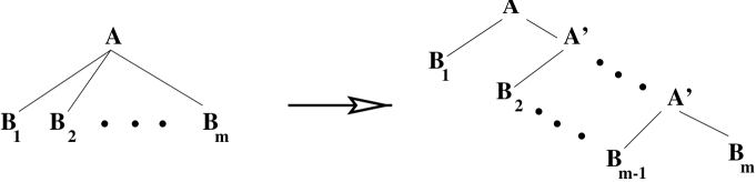
Figure 15: An approximation of the CNF transformation

Given these two observations, the ACNF transformation starts by assigning to every elementary-tree of the STSG a unique address from a domain $\Pi$. During the ACNF transformation, every elementary-tree retains its address. The ACNF transformation has the following steps:

• Transform the elementary-trees of $G_{stsg}$ to elementary-trees containing no unary productions.

• Transform the elementary-trees, resulting from the preceding transformation, to a form where every node, in every elementary-tree, has either children that are all non-terminals or has one single terminal child.

• Transform every resulting elementary-tree to CNF by traversing it from its root to its leaves in a breadth-first traversal. Under every node in the elementary-tree, encountered during the traversal, there is now a production rule; if the production rule is not in CNF then it must be a rule ${A\rightarrow B_{1}\cdots B_{m}}$, where $m>2$ and all $B_{i}$ is a non-terminal. Transform this rule into a right linear (or left linear) structure by introducing exactly $m-2$ nodes labelled with the same fresh symbol $A^{{}^{\prime}}$. Figure 15 depicts this step.

The tree- and string-sets of the resulting CNF CFG are supersets of the respective sets of the CNF STSG. In fact, the ACNF transformation results in a CNF CFG that behaves in two different ways: internal to elementary-trees as a right-linear grammar (a regular grammar) and external to elementary-trees as a CFG.

It is important here to restate two simple facts, mentioned above, and sketch their proof informally:

Proposition 5.1

The ACNF transformation results in a CNF STSG with the same string language as the original STSG $G_{stsg}$. Moreover, up to a simple reverse transformation, the tree language of the CNF STSG is equal to that of $G_{stsg}$.

Proof 5.1:

The transformation alters only the internal structure of elementary-trees, i.e. it does not alter the root node or the leaf nodes and their labels. Exactly the same derivations, substition sequences of elementary-trees together with their unique addresses, are still possible in the CNF STSG as the original STSG. Thus the string language of the CNF STSG is the same as that of the original STSG. A simple reverse-transformation gives back the same tree language also. Text books on parsing exhibit for the first two transformations reverse transformations, e.g. [Aho and Ullman, 1972]. For the third step, a reverse transformation simply removes every node labeled with $A^{{}^{\prime}}$, where $A$ is a non-terminal of the STSG and uses the unique addresses in order to retrieve the original structures  $\Box$

Proposition 5.2

The string/tree language of the CFG underlying the STSG $G_{stsg}$, i.e. $G_{cfg}$, is a subset of (respectively) the string/tree language of the CNF CFG (underlying the CNF STSG resulting from the approximate CNF transformation).

Proof 5.2:

It can be eaily observed that every derivation of $G_{cfg}$  is still possible in the ACNF CFG resulting from the transformation. However, the ACNF CFG might have extra non-terminals introduced during the transformation. This introduces new derivations for (possibly) other strings and other trees  $\Box$

As mentioned earlier, the string/tree language of an STSG is always a subset of (respectively) the string/tree language of the CFG underlying it. Together with the above two facts this means that the tree/string language of the original STSG is respectively a subset of the tree/string language of the CNF CFG.

The ACNF transformation introduces new rules. The number of the newly introduced rules is at most equal to the sum of the lengths of the right hand sides of the rules of the CFG underlying the STSG, i.e. $O(|G_{cfg}|)$. The number of non-terminals has grown but it is at most double that of the CFG $G_{cfg}$. In this way, we have a small CNF grammar of the same order of magnitude as the original CFG $G_{cfg}$. For linguistic CFGs, the right hand sides of rules are much shorter than the lengths of frontiers of elementary-trees of DOP STSGs. And besides, some of the newly introduced rules have more chance to be identical than in transforming the STSG into CNF, implying even a smaller grammar. Most importantly, the ACNF transformation, even in the worst-case, does not result in squaring the size of the CFG. All in all, this approximation of the CNF results in a small grammar that can be parsed very fast using the CKY.

The transformation results also in a CNF STSG that has new nodes in its elementary-trees. As explained above, the number of the new nodes is in the worst case equal to the length of the frontiers of the elementary-trees, i.e. $O(|A|)$, where $|A|$ is the total number of nodes in the elementary-trees of the STSG. This doubles the number of nodes in the worst-case, but the CNF approximation introduces only $O(|G_{cfg}|)$ new non-terminals (as opposed to $O(|A|)$ in the usual CNF transformation, as explained earlier).

26.3 STSG-derivations recognition

Be given an STSG $G_{stsg}$ $=$ ($V_{N}$, $V_{T}$, $S$, ${\cal C}$, $PT$)  in CNF (the transformation to CNF is as described above). The input sentence is denoted $w_{0}^{n}$, where $w_{0}=\epsilon$. The present algorithm has the structure:

Phase 1.

Apply the CKY algorithm using the (CNF) CFG underlying $G_{stsg}$, denoted $G_{cfg}$, resulting in a parse-forest of the input sentence. As mentioned above, this parse-forest is a superset of the parse-forest which $G_{stsg}$ spans for the same sentence.

Phase 2.

Apply an algorithm, described below, for computing the parse-forest of $G_{stsg}$ from the approximate parse-forest of the previous phase, and compute the MPD on this parse-forest.

Often, I will refer to the first phase with the general term “parsing phase” and to the second phase with the term “disambiguation-phase”. Both terms do not reflect the exact task of each phase. They only reflect the main task of each phase: (approximating) parse-forest generation in the first, and computation of the MPD, i.e. the selection of one preferred tree from the exact parse-forest, in the second.

Below I discuss the second phase, which fulfils three requirements: preserve atomicity of $G_{stsg}$’s elementary-trees, preserve the uniqueness of every elementary-tree, and recognize exactly $G_{stsg}$’s parse-forest and derivations for the input sentence from the CFG parse-forest. But first I discuss the issue of how to recognize a derivation of $G_{stsg}$ when given a parse-forest of $G_{cfg}$. The issue of recognizing an STSG derivation is central in the MPD-computation algorithm. But first the following definitions.

Node address:

This is a unique address from some domain $\Pi$ assigned to a non-leaf node in an elementary-tree of $G_{stsg}$.

Every non-leaf node in every elementary-tree of $G_{stsg}$is assigned such a unique node-address from $\Pi$. It is useful if the addresses of the nodes of an elementary-tree enable fast checking of the parent-child (and the number of the child if counting from left to right) and sisterhood relations between nodes in an elementary-tree.

Decorated tree:

A tree in which every non-leaf node is decorated with exactly one address, from the STSG elementary-trees’ node addresses, is called a decorated tree. The collection of node addresses in a decorated tree is called the decoration of that tree.

Derivation-tree:

Every derivation of the STSG can be characterized by a unique decoration of the tree it generates; in this decoration every node in the tree is decorated with the unique address of the corresponding node of an elementary-tree. We refer to this decorated tree with the term derivation-tree.

   

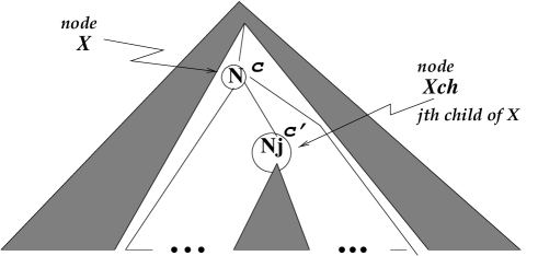
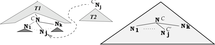
Figure 16: (Top) decorated tree, (bottom) the viability property

Note that not every decorated tree is a derivation-tree since some decorations do not correspond to STSG derivations. We observe that a simple algorithm can be used for recognizing whether a decorated tree is a derivation-tree of $G_{stsg}$ or not. To this end, we need to define the viability property, a main element of this algorithm and the algorithm for computing the MPD.

Viability property:

Let $X$ be a node in a decorated-tree, labeled $N$ and decorated with address $c$, and let $Xch$ be its $j$th child-node, labeled $N_{j}$ and decorated with address $c^{{}^{\prime}}$, $j\in\{1,2\}$. We say that the viability property holds for nodes $X$ and $Xch$ if one of the following two holds (see figure 16):

Parenthood:

There is some elementary-tree, in $G_{stsg}$, for which $c$ and $c^{{}^{\prime}}$ correspond to two of its non-leaf nodes that are related (respectively) as parent and its $j$th child. Moreover the node corresponding to $c$/$c^{{}^{\prime}}$ in that elementary-tree is labeled respectively with $N$/$N_{j}$.

Substitution:

There is some elementary-tree, in $G_{stsg}$, for which the address $c$ corresponds to one of its nodes that is labeled $N$ and that has a leaf child-node labeled with a non-terminal $N_{j}$, i.e. a substitution-site. And there is some elementary-tree, in $G_{stsg}$, for which the address $c^{{}^{\prime}}$ corresponds to its root node that is labeled $N_{j}$.

The algorithm for recognizing whether a decorated tree is a derivation-tree of $G_{stsg}$ is shown is figure 17; we will refer to it with the name algorithm 17.

 

Root:

Check whether the root of the tree is labeled $S$ and is decorated with an address which corresponds to the root of an elementary-tree. If not then goto Fail below.

Iterate:

For every node in the decorated tree, that is not a leaf node, do:
1) let that node be the current node,
2) for the current node $X$, labeled $N$ and decorated with address $c$, and its $j$th child-node $Xch$, labeled $N_{j}$ and decorated with address $c^{{}^{\prime}}$, $j\in\{1,2\}$, check that the viability property holds for $X$ and $Xch$, otherwise goto Fail.

Accept:

return accept and exit.

Fail:

return reject and exit.

 

Figure 17: Algorithm 17: Recognizing a derivation-tree

The following propositions express the role which the viability property plays in recognizing derivation-trees.

Proposition 5.3

If a decorated tree contains a node that does not fulfill the viability property, the decorated tree is not a derivation-tree of the STSG at hand.

Proposition 5.4

Algorithm 17 recognizes a decorated tree iff it is a derivation-tree of the STSG at hand.

The proofs of these two propositions are simple to construct and will be skipped here.

As a result to the propositions above, if given a parse-forest, spanned by the STSG $G_{stsg}$ for some input sentence, it is possible to determine the set of all derivation-trees of the sentence by applying the above algorithm to the parse-forest. However, applying this algorithm blindly would result in exponential time-complexity. It is necessary to apply it in an efficient manner. Moreover, instead of applying the recognition of the derivation-trees of a sentence to $G_{stsg}$’s parse-forest, we may apply it to the CFG’s parse-forest; this determines the derivation-trees of the sentence according to the STSG $G_{stsg}$ and, as a side effect, this delimits $G_{stsg}$’s parse-forest for the sentence, since trees without $G_{stsg}$’s derivation-trees are not trees of $G_{stsg}$.

To obtain a (deterministic) polynomial-time algorithm for the recognition of the set of derivation-trees of an input sentence, we employ a new compact structure, in analogy to a parse-forest, called a derivation-forest of the sentence. To this end, define:

Rule occurrence:

Let rule $R\in$ ${\cal R}$ be found under a non-leaf node with address $c$ of some elementary-tree. The address $c$ is called an occurrence of $R$ in that elementary-tree. An occurrence of an item $A$$\rightarrow$$\alpha\bullet\beta$ is an occurrence of the rule ${A\rightarrow\alpha\beta}$.

Occurrence set:

The occurrence set, denoted ${\cal A}(R)$, of rule $R\in$ ${\cal R}$ is the set of all occurrences of $R$ in all elementary-trees of $G_{stsg}$.

Item’s occurrences set:

Let $A$$\rightarrow$$\alpha\bullet\beta$ $\in$ $[i,j]$. The occurrences set of this item is defined as ${\cal A}(A\rightarrow\alpha\bullet\beta,~{}i,~{}j)$ = ${\cal A}({A\rightarrow\alpha\beta})$.

Given the CFG parse-forest and the CKY table of the input sentence, built by the CKY algorithm, a decoration of the items in the table enables recognizing the derivation-forest of that sentence. We maintain with every item its occurrence set. The derivation-forest is constructed on top of the CFG parse-forest, also in a bottom-up fashion by applying an algorithm for recognizing derivation-trees to the occurrence sets of the items that are connected together in the parse-forest by the $AddedBy$ relation described in the previous section. Similar to our presentation of the Viterbi CKY, we do not show exactly how to construct the derivation-forest, instead we show how to compute the MPD of the input sentence. The construction of the derivation-forest extends the MPD algorithm described below only by associating sets of pointers between occurrences of items. Recall that if an item $B$ results in adding another item $A$ to entry $[i,j]$, during Deduce of CKY, then $B\in AddedBySet_{A,i,j}$, where this expresses a pointer from $A$ to $B$. Similarly, a set is associated with every occurrence, $c$, of $A$, denoted $ViabilitySet_{c,A}$. If $B\in AddedBySet_{A,i,j}$ and $b$ is an occurrence of $B$, then $b\in ViabilitySet_{c,A}$ iff a predicate $Viable?(c,b,j)$, defined below, is true; except for final binary items, $j$ is always equal to 1. For final binary items, the value $j\in\{1,2\}$ allows testing the predicate $Viable?(c,b,j)$ for the left (“first child”) or right (“second child”) items in the pairs of items in $AddedBy$ of the final binary item. The predicate $Viable?$ tests the viability property defined earlier for the algorithm 17 for recognizing derivation-trees.

26.4 Computing the MPD

For computing the MPD of an input sentence under $G_{stsg}$, it is useful to precompile the $G_{stsg}$ into a form that makes the viability property explicit. To this end, infer the following predicates and functions from $G_{stsg}$$=$ ($V_{N}$, $V_{T}$, $S$, ${\cal C}$, $PT$):

1. $Parent?(c,~{}c^{{}^{\prime}},~{}j)$ denotes the proposition “$c$ and $c^{{}^{\prime}}$ are the addresses of a parent and its $j$-th child in an elementary-tree in ${\cal C}$”.

2. $Root?(c)$ denotes the proposition “$c$ is the address of the root node of an elementary-tree in ${\cal C}$”.

3. $TreeOf(c)$ denotes the function that returns $t\in$${\cal C}$such that $c$ is the address of some node in $t$.

4. $SubSite?(c,j)$ denotes the proposition “child nr. $j$ of the node with address $c$, in some elementary-tree, is a substitution-site”.

Then infer the eight-tuple ($V_{N}$, $V_{T}$, $S$, ${\cal R}$, $\cal A$, $Viable?$, $P$, $PF$), from $G_{stsg}$, where:
$\bullet$ ($V_{N}$, $V_{T}$, $S$, ${\cal R}$)  is the CFG underlying ($V_{N}$, $V_{T}$, $S$, ${\cal C}$, $PT$), $\bullet$ $\forall$ $R\in{\cal R}$:  ${\cal A}(R)$ = $\{c~{}|c$ is the address of an occurrence of $R\},$ $\bullet$ $Viable?(c,~{}c_{j},~{}j)$  =  $Parent?(c,c_{j},j)$  or  $(~{}SubSite?(c,j)$  and  $Root?(c_{j})~{})$, $\cal A$ = {$\cal A$$(R)$ $|$ $R\in$ ${\cal R}$}, $\bullet$ $P$ : $\Pi$ $\rightarrow$$(\Pi\times\{1,2\})$ $\rightarrow$$[0..1]$, For $c,c^{{}^{\prime}}\in\Pi$ and $j\in\{1,2\}$: $P(c)(c^{{}^{\prime}},j)$ = $\left\{\begin{tabular}[]{ll}$PT(TreeOf(c))$&[$j=2$ {\footnotesize\bf and}~{} $Viable?(c,c^{{}^{\prime}},j)$ {\footnotesize\bf and}~{} $Root?(c)$]\\ {\bf 1}&[$Viable?(c,c^{{}^{\prime}},j)$ {\footnotesize\bf and}~{} ($j=1$ {\footnotesize\bf or}~{} {\bf not} $Root?(c)$)]\\ {\bf 0}&[{\bf otherwise}~{}],\\ \end{tabular}\right.$ $\bullet$ $PF$ : $\Pi$ $\rightarrow$$[0..1]$, for $c\in\Pi$: $PF(c)$ = $\left\{\begin{tabular}[]{ll}$PT(TreeOf(t))$&[$Root?(c)$]\\ {\bf 1}&[~{}{\bf not} $Root?(c)$]\\ \end{tabular}\right.$

The predicate $Viable?()$ formalizes the viability property. For a decorated tree, in which $c$ decorates a node $X$, the term $P(c)$ denotes the probability of $c$ as a function of the address $c^{{}^{\prime}}$ of the $j$th child of $X$ (counting children is always from left to right).This definition enables writing the algorithm as a recursive function. $P$ expresses the probabilities in terms of the “probabilities” of the rules of the CFG underlying $G_{stsg}$; the probability of a rule of the CFG underlying $G_{stsg}$ is a function of its particular occurrence, i.e. address, in the elementary-trees set of $G_{stsg}$.

 

$$\begin{array}[]{rl}&\\ P_{mpd}(w_{0}^{n})=&{\bf Max}_{\tiny\begin{tabular}[]{l}\mbox{$S$$\rightarrow$$\alpha\bullet$$\in\mbox{[0, n]}$}\\ \mbox{$c\in{\cal A}(S\rightarrow\alpha\bullet,~{}0,~{}n)$}\\ \mbox{and $Root?(c)$}\\ \mbox{}\\ \end{tabular}}Pp(c,~{}S\rightarrow\alpha\bullet,~{}0,~{}n)\\ \mbox{ }&\\ Pp(c,item,i,j)=&{\bf case}~{}item~{}{\bf of{}}\\ \mbox{ }&\\ A\rightarrow w_{i+1}\bullet:&PF(c),~{}~{}~{}$where$~{}$j = i+1$,\\ \\ A\rightarrow B\bullet C:&\overbrace{{{\bf Max}}_{\alpha}{{\bf Max}}_{c1\in{\cal A}(B\rightarrow\alpha\bullet,i,j)}P(c)(c1,1)\times Pp(c1,B\rightarrow\alpha\bullet,i,j)},\\ \\ A\rightarrow BC\bullet:&{\bf Max}_{i<k<j}~{}Pp(c,A\rightarrow B\bullet C,i,k)~{}\times\\ &\overbrace{{\bf Max}_{\alpha}{\bf Max}_{c2\in{\cal A}(C\rightarrow\alpha\bullet,k,j)}P(c)(c2,2)\times Pp(c2,C\rightarrow\alpha\bullet,k,j)}\end{array}$$

Figure 18: Algorithm 18 for computing the MPD of a sentence $w_{0}^{n}$

 

Let ${\bf Max}_{Pred(x)}A(x)$ denote the maximum of the set {$A(x)$ /  $Pred(x)$}. The algorithm for computing the MPD of a sentence $w_{1}^{n}$ is shown in figure 18, also referred to as algorithm 18. It computes the MPD of the input sentence on the parse-forest, which was constructed in the first phase by the CKY of the CFG $G_{cfg}$. The function $P_{mpd}(w_{0}^{n})$ computes the probability of the MPD of the sentence $w_{0}^{n}$, where $w_{0}=\epsilon$. The function $Pp:~{}\Pi\times~{}ITEMS\times~{}[0,~{}n]\times~{}[0,~{}n]\rightarrow~{}[0,~{}1]$ computes recursively the probability of the most probable among the “partial-derivations”, that start with address $c$ and generate a partial-tree for $w_{i}^{j}$.

Note that for SCFGs, i.e. when the elementary-trees of $G_{stsg}$have no internal nodes, the algorithm in figure 18 computes the MPD exactly as algorithm 14. This becomes more obvious if one notices that the probability function $P(c)$ always computes to $PT(t)$ or $1$, due to the fact that the elementary-trees have no internal nodes at all. For the general case of STSGs, a proposition and its proof, following the next definitions, take care of the correctness of the present algorithm.

Partial derivation-tree:

A partial derivation-tree of an STSG is a partial-tree, resulting from a partial-derivation of the CFG underlying that STSG, in which each node is decorated with a node-address such that the viability property still holds for each of the nodes.

A partial derivation-tree consists of, on the one hand, a sequence of elementary-tree substitutions, and on the other hand, other “pieces” of elementary-trees. A piece is a decorated subtree, of an elementary-tree, that either contains the root or some leaf-nodes of that elementary-tree but not both. The elementary-trees and the pieces in the partial derivation-tree are combined with substitution under the STSG’s viability property, i.e. substitution is allowed only of a node that has the address of a root of an elementary-tree on a node that originally was a substitution-site in an elementary-tree.

We will say that an elementary-tree fully participates in a partial derivation-tree $DT$ iff the addresses of all its nodes decorate nodes in $DT$. And we will say that an elementary-tree partially participates in a partial derivation-tree $DT$ iff the addresses of some of its nodes do not decorate a node in $DT$, but the addresses of the other nodes do decorate nodes in $DT$.

Sub-derivation:

For every partial derivation-tree there is exactly one corresponding sequence of substitutions, of both the elementary-trees that fully and those that partially participate in that partial derivation-tree; this sequence is denoted with the term the sub-derivation corresponding to the partial derivation-tree.

In particular, a derivation of the STSG is a sub-derivation 1) that starts with an elementary-tree with a root node labeled $S$, 2) that has leaf nodes labeled with terminals and 3) in which every elementary-tree fully participates.

Probability of a sub-derivation:

The probability $Pp(DT)$ of a sub-derivation $DT$ is equal to the product of the probabilities of all elementary-trees that fully participate in it. The probability of a partial derivation-tree is equal to the probability of the corresponding sub-derivation.

Thus, a partial derivation-tree corresponds to some “acceptable” decoration of a partial-tree’s nodes. The viability property determines the “acceptable” decorations that corresponds to actual sub-derivations of the given STSG. The algorithm in figure 18, in short algorithm 18, exploits the viability property by assigning zero probability to non-acceptable decorations and the right probability to the acceptable decorations.

Proposition 5.5

$\forall~{}item\in$ $[i,j]$, $0\leq i<j\leq n$, and $\forall~{}c\in{\cal A}(item,i,j)$, $Pp$ fulfills one of two:

• $Pp(c,item,i,j)$, is equal to the maximum probability of all possible partial derivation trees $dt$ of $w_{i}^{j}$, that fulfill

  • if $item=$$A$$\rightarrow$$\alpha\bullet$ then $dt$ has a root node labeled $A$, decorated with $c$, and has children labels that (when concatenated from left to right) form a string equivalent to $\alpha$,

  • if $item=$$A$$\rightarrow$$B\bullet C$ then $dt$ has a root node labeled $B$ and decorated with $c^{{}^{\prime}}$ such that $Viable?(c,c^{{}^{\prime}},1)$ is true.

• There are no such partial derivation-trees as in the preceding case and $Pp(c,item,i,j)$ is equal to zero.

Proof 5.5:

The proof is by induction on $x$, $1\leq x=(j-i)<n$. It depends partially on the CKY property that $A\rightarrow\alpha\bullet\beta\in[i,j]$ iff ${A\rightarrow\alpha\beta}$ $\stackrel{{\scriptstyle*}}{{{\rightarrow}}}$$w_{i}^{j}\beta$.

${\bf x=1:}$

Then $\alpha=w_{i+1}$. By the CKY property, in this case there is at most one possible partial derivation-tree, i.e. ${A\rightarrow w_{i+1}}\in{\cal R}$ with $A$ decorated with $c$. Therefore, $Pp(c,A\rightarrow w_{i+1}\bullet,i,i+1)=PF(c)$. The proposition holds since there is only one partial-derivation tree.

${\bf x=m:}$

Assume the proposition holds for all $1\leq x\leq m$, $m<n$.

${\bf x=m+1:}$

Let $A$$\rightarrow$$\alpha\beta\bullet$ $\in$ $[i,j]$ and $c\in{\cal A}({A\rightarrow\alpha\beta})$. By the CKY property there is a partial CFG-derivation (or many such derivations) ${A\rightarrow\alpha\beta}$ $\stackrel{{\scriptstyle*}}{{{\rightarrow}}}$$w_{i}^{j}\beta$. Now there are two cases:

$\alpha=BC,\beta=\epsilon$:

Again by the same CKY property, for every partial CFG-derivation ${A\rightarrow BC}$ $\stackrel{{\scriptstyle*}}{{{\rightarrow}}}$$w_{i}^{j}$, there is $i<k<j$ such that there are two partial CFG-derivations: ${A\rightarrow BC}$ $\stackrel{{\scriptstyle*}}{{{\rightarrow}}}$$w_{i}^{k}C$ and $C$ $\stackrel{{\scriptstyle*}}{{{\rightarrow}}}$$w_{k}^{j}$. The proof now is for every $i<k<j$ for which this is true. For the current value of $k$, let us consider the probabilities of the possible decorations, of the partial CFG-derivation of $w_{i}^{j}$ at hand, that have $c$ decorating $A$ in $A$$\rightarrow$$BC\bullet$. As explained above, with every such decoration there are (at least) two decorated partial CFG-derivations for $w_{i}^{k}$ and $w_{k}^{j}$. By the CKY property and the inductive assumption three things hold for these pairs of decorations:

1. for all $\gamma$, for all $cb\in{\cal A}({B\rightarrow\gamma})$, $Pp(cb,B\rightarrow\gamma\bullet,i,k)$ is equal either to zero or to the maximum probability of all partial derivation-trees of $w_{i}^{k}$ starting at ${B\rightarrow\gamma}$ with $B$ decorated with address $cb$.

2. $Pp(c,A\rightarrow B\bullet C,i,k)$ is equal either to zero or to the maximum probability of any partial derivation-tree of $w_{i}^{k}$ starting at ${B\rightarrow\gamma}$ with $B$ decorated with address $cb$ and $Viable?(c,cb,1)$ is true.

3. for all $\delta$, for all $cc\in{\cal A}({C\rightarrow\delta})$, $Pp(cc,C\rightarrow\delta\bullet,k,j)$ is equal either to zero or to the maximum probability of any partial derivation of $w_{k}^{j}$ starting at ${C\rightarrow\delta}$ with $C$ decorated with address $cc$.

If $Pp(c,A\rightarrow B\bullet C,i,k)$ is zero for the current value of $k$, then $Pp(c,A\rightarrow BC\bullet,i,j)$ is also zero. By the inductive assumption we conclude that there is no partial derivation-tree starting at $A$$\rightarrow$$BC\bullet$ and where $A$ is decorated with $c$, for the current value of $k$. If it is not zero, we face two cases for all $\delta$ and for all $cc\in{\cal A}({C\rightarrow\delta})$:

1. $Viable?(c,cc,2)$ is false: then $P(c)(cc,2)=0$

2. $Viable?(c,cc,2)$ is true: $P(c)(cc,2)$ is either $PT(TreeOf(c))$ or $1$, depending on whether $Root?(c)$ is true or not.

The last case in the switch of algorithm 18 (case $A$$\rightarrow$$BC\bullet$) takes the maximum of all $P(c)(cc,2)\times Pp(cc,C\rightarrow\delta\bullet,k,j)$, for all $\delta$ and for all $cc\in{\cal A}({C\rightarrow\delta})$. By the inductive assumption and the viability property and the definition of partial derivation-trees, this is equal either to zero or to the maximum probability of all partial derivation-trees starting at $A$$\rightarrow$$BC\bullet$ with address $c$, for this value of $k$. Again by the inductive assumption, multiplying this with $Pp(c,A\rightarrow B\bullet C{},i,k)$ and maximizing this for all values of $k$ proves the proposition for this case.

$\alpha=B,\beta=C$:

The proof for this case follows a similar line of argumentation as the preceding case.    $\Box$

Proposition 5.6

Algorithm 18 computes the MPD of $w_{1}^{n}$ under $G_{stsg}$.

Proof 5.6:

Easy to derive from algorithm 18, proposition 5.5 and the unique correspondence between derivation-trees and STSG derivations.   $\Box$

Complexity:

The time complexity of the second phase of the algorithm is $O(|{\cal A}|^{2}\times n^{3})$. And the time complexity of the first phase is $O(|{\cal R}|\times n^{3})$. For DOP STSGs $|{\cal R}|$, the size of the CFG underlying the STSG, is usually in the order of $1\%$ of $|{\cal A}|$. Therefore in practice the algorithm given above behaves as if having time-complexity $O(|{\cal A}|^{2}\times n^{3})$. However, a simple optimization, discussed below, reduces the time-complexity of the second phase to $O(|{\cal A}|\times n^{3})$. Moreover, the algorithm computes the second phase on the result of the first phase, i.e. a parse-forest that already pruned many of the failing STSG derivations. This saves space and time that are expected to be much larger than the small overhead of having a first and a second phase. The net effect is faster computation that uses smaller space.

Derived algorithms:

Algorithm 18 can be easily modified to result in other useful algorithms. To compute the probability of the input sentence, as the sum of the probabilities of all its derivations, exchange ${\bf Max}$ with the operator $\sum$ everywhere in the specification of the algorithm. For computing the MPD and the probability of a given parse-tree, the first phase of the algorithm is exchanged for a small algorithm that transforms the parse-tree into a CKY table with items in the entries; the second phase is applied as is either with ${\bf Max}$ or with $\sum$, depending on the algorithm wanted.

Implementation issues:

It is important to note that, for clarity of presentation, the specification given in figure 18 is not as efficient as the algorithm can be implemented. For implementing the second phase of the algorithm, one precompiles the STSG, as explained above, in order to make the viability property tables explicit. The second phase is applied on the parse-forest in a bottom-up fashion (rather than top-down recursion as the specification does) making use of the $AddedBy$ sets of the items in the parse-forest of the first-phase. Moreover, failing sub-derivations, which have probability zero, are discarded (rather than dragged together with the others all the way).

26.5 Optimization: approaching linearity in STSG size

Here we discuss an important optimization of algorithm 18, based on the following property of STSGs:

Paths:

A sequence of nodes, i.e. pairs of labels and addresses, starting at the root node of a derivation-tree and terminating at a leaf node (labeled with a terminal symbol) is called a path of the derivation-tree.

Path set:

The path set of a derivation-tree is the set of all paths in that derivation-tree. The path set of a given tree is the union of the path sets of all derivations that generate the tree under the STSG at hand. Similarly, the path set of a sentence is the union of all path sets of the derivations that generate it under the STSG at hand. The path set of the STSG is the union of the path sets of the sentences in its string language.

Relevant property:

The path set of an input sentence under a TSG is a regular language. This property is known to be true for CFGs [Thatcher, 1971] and can be easily proved for TSGs.

This property implies that recognition of the path set, and also the derivations, of an input sentence under an STSG should be possible in time complexity linear in the number of possible node-labels and their addresses, i.e. $|{\cal A}|$. A simple observation, related to the viability property, makes this even clearer: in an elementary-tree, a node labeled $A$ with address $c$ can be only in one of the following two configurations:

• $SubSite?(c,j)$ is true, i.e. the $j$th child of $c$ is a substitution-site in the elementary-tree (i.e. a frontier non-terminal). In this configuration, $Viable?(c,cj,j)$ is true only for all $cj$ such that $Root?(cj)$.

• $Parent?(c,cj,j)$ is true for some $cj$, i.e. $c$ and $cj$ are both non-leaf nodes in the elementary-tree and are respectively the addresses of a parent and its $j$th child in that elementary-tree. Only one single $cj$ fulfills this (due to the unique addresses of nodes in elementary-trees).

Let $itemP$ denote any item to the left of the semicolon in algorithm 18. And let $itemCh$ denote any item found in the overbraced term also in algorithm 18. The algorithm checks the viability of every address $c\in{\cal A}(itemP)$ with address $cj\in{\cal A}(itemCh)$. The above observation says that this is unnecessary since there are only two complementary configurations in which $c$ and $cj$ fulfill the viability property. In fact it says even that $c\in{\cal A}(itemP)$ can be in one of two configurations, and $cj\in{\cal A}(itemCh)$ can also be in one of two corresponding configurations. This motivates partitioning ${\cal A}(itemP)$ and ${\cal A}(itemCh)$ into:

$$HasSubSite(itemP,j) = \{c\in{\cal A}(itemP)~{}|~{}SubSite?(c,j)~{}is~{}true\},$$

$$HasChild(itemP,j) = {\cal A}(itemP)~{}-~{}HasSubSite(itemP,j),$$

$$RootsOf(itemCh) = \{cj\in{\cal A}(itemCh)~{}|~{}Root?(cj)~{}is~{}true\},$$

$$InternOf(itemCh) = {\cal A}(itemCh)~{}-~{}RootsOf(itemCh)$$

Recall that the viability property states that:

$Viable?(c,cj,j)$ is true for $c\in{\cal A}(itemP)$ and $cj\in{\cal A}(itemCh)$ iff either [$c\in HasSubSite(itemP,j)$ and $cj\in RootsOf(itemCh)$] or [$c\in HasChild(itemP,j)$ and $cj\in InternOf(itemCh)$].

The above mentioned observation extends it and states that:

For every $c\in HasSubSite(itemP,j)$ and every $cj\in RootsOf(itemCh)$ holds $Viable?(c,cj,j)$ is true. And, for every $c\in HasChild(itemP,j)$, there is at most one $cj\in InternOf(itemCh)$ such that $Viable?(c,cj,j)$ is true.

For both cases it is possible to conduct the computation for every $c\in itemP$ in $O(1)$ rather than $O(|{\cal A}|)$ (i.e. $|{\cal A}(itemCh|)$). In the first case, compute only once the set $RootsOf(itemCh)$ and its maximum probability and pass this to every $c\in HasSubSite(itemP,j)$. In the second case, an off line precompilation of the place of the $j$th child, for $j\in\{1,2\}$, of every $c\in HasChild(itemP,j)$ in ${\cal A}(R)$, for every $R$ enables finding it in $O(1)$; then the maximum probability of the $j$th child is passed to $c$ for computing its maximum probability in $O(1)$.

More formally, the overbraced expression in figure 18 in each of the last two cases of algorithm 18 is rewritten. Let these two expressions be represented by the more general expression

$${{\bf Max}}_{\alpha,~{}c_{l}\in{\cal A}(itemCh,m,q)}P(c)(c_{l},l)\times Pp(c_{l},itemCh,m,q).$$

Substitute for this expression the following, where $item,i$ and $j$ are as defined by algorithm 18:

$$\left\{\begin{array}[]{lll}{\bf if}~{}~{}(c\in HasSubSite(item,l))&:&PF(c)\times\\ &&{{\bf Max}}_{\alpha,~{}c_{l}\in RootsOf(itemCh)}Pp(c_{l},itemCh,m,q),\\ {\bf if}~{}~{}(c\in HasChild(item,l))&:&PF(c)\times\\ &&{\bf if}~{}~{}{\bf(~{}}\exists c_{l}\in InternOf(itemCh):~{}Parent?(c,c_{l},l){\bf~{})}\\ &&{\bf then}~{}~{}{{\bf Max}}_{\alpha}Pp(c_{l},itemCh,m,q)\\ &&{\bf else}~{}~{}~{}~{}0.\\ \end{array}\right.$$

Both cases in this specification must be implemented as explained above in order to achieve linearity in $|{\cal A}|$ during the second phase of the algorithm. The time complexity of the algorithm (two phases) is now proportional to $(|{\cal R}|+|{\cal A}|)\times n^{3}$. As mentioned earlier, $\frac{|{\cal R}|}{|{\cal A}|}$ is very small for DOP STSGs. Therefore, the time complexity actually approaches $O(|{\cal A}|\times n^{3})$ as $\frac{|{\cal R}|}{|{\cal A}|}$ approaches zero. For most DOP STSG the actual time complexity indeed approaches the linear in STSG size. This optimization does not result in any change in the space complexity, which remains $O((|R|+|{\cal A}|)\times n^{2})$.

It is interesting to observe the effect of this optimization in practice. To this end, I conducted a preliminary experiment comparing various versions of the algorithm: a linear version in STSG size, a square version and a version that searches for the child of each address using Binary-Search on ordered arrays. The results are listed in Table 1. The experiments reported in table 1 used the ATIS domain Penn Tree-bank version 0.5 (Penn TreeBank Project, LDC) without modifications. They were carried out, on a Sun Sparc station 10 with 64 MB RAM, parsing ATIS word-sequences. The three versions were compared for execution-time by varying STSG sizes on the same test set of 76 sentences, randomly selected. The sizes of the STSGs were varied by varying the allowed maximum depth of elementary-trees and by projecting only from part of the tree-bank in some other cases (with a maximum of 750 training trees). Average cpu-time includes parse-forest generation, i.e. both phases. It is clear that there is a substantial difference in growth of execution-time between the three versions as grammar size grows. Note also that this experiment exemplifies, to some extent, the ratio between $|R|$ and $|A|$ for ATIS DOP STSGs. These observations hold also for experiments with DOP on other domains, reported in chapter 6.

 

num. of	$|$${\cal R}$$|$	$|{\cal A}|$	Avg.Sen.	Average CPU-secs.
elem. trees			Length	linear	Bin.Search	Square
74450	870	436831	9.5	445	993	9143
26612	870	381018	9.5	281	$-$	$-$
19094	870	240619	9.5	197	$-$	2458
19854	870	74719	9.5	131	223	346

Table 1: Disambiguation times for various STSG sizes

 

26.6 Extension for disambiguating word-graphs

The two-phase algorithm for parsing and disambiguating sentences under STSGs can be easily extended for parsing and disambiguating word-graphs as those produced by speech recognizers. As mentioned in chapter 2 a word-graph is a Stochastic Finite State Machine (FSM). For notation and definitions on word-graphs, the reader is referred to chapter 2.

Assumptions:

In this work we assume FSMs and SFSMs that contain no cycles, i.e. paths $s_{x}\cdots s_{x}$ $\stackrel{{\scriptstyle*}}{{{\rightarrow}}}$$w_{1}^{n}$, for $n\geq 1$. Due to the preceding assumption we may assume, without loss of generality, that the set of states $\Sigma$, of SFSM $(Q,\Sigma,S,T,F,P)$, is equal to the set of numbers $\{0,1,\cdots(|\Sigma|-1)\}$ such that: 1) each transition $\langle s1,s2,w\rangle$ fulfills $s1<s2$, 2) the start-state $S$ is $0$, and 3) the target state is $(|\Sigma|-1)$.

Before discussing how to parse and disambiguate word-graphs under DOP STSGs, it is clarifying to note that a sentence $w_{1}^{n}$ is also a simple word-graph. The CKY algorithm exploits this by numbering a position between the words $w_{i}$ and $w_{i+1}$, for all $1\leq i\leq n$, by the number $i$. It also numbers the position before the first word by $0$. These are the states of a word-graph with the transitions $\langle i-1,i,w_{i}\rangle$, for all $1\leq i\leq n$. Note that in a sentence, every transition is from a state $i$ to the state $i+1$. In general word-graphs this is not the case; transitions can be from any state $i$ to any state $j>i$.

Parsing an FSM with a CFG is known in the literature as the problem of computing the intersection of the two machines; studies of algorithms for conducting this intersection are discussed in e.g. [van Noord, 1995]. Below I discuss how to extend the two-phase MPD computation algorithm under STSGs for word-graphs, i.e. SFSMs. Firstly I discuss how to extend the CKY parser of the first phase for this task in a similar fashion to preceding work. After that, I discuss how to compute the MPD of an SFSM under an STSG, in the second phase of the present algorithm.

Assume again that we are given the STSG $G_{stsg}$= ($V_{N}$, $V_{T}$, $S$, ${\cal C}$, $PT$)  in CNF, and let $G_{cfg}$= ($V_{N}$, $V_{T}$, $S$, ${\cal R}$)denote the CFG underlying it. Moreover, let $WG$ denote the wordgraph $(Q,\Sigma,S,T,F,P)$ where $\Sigma=$$\{0,\cdots M\}$, $M\geq 1$, $Q=\{w_{i}|1\leq i\leq X\}$, and $S$ denotes $0$ and $F$ denotes $M$. For the rest of this section, we assume that $Q\subseteq$$V_{T}$ holds.

26.6.1 First phase

Recall that when the CKY algorithm parses the sentence $w_{1}^{n}$ under a CFG, it maintains the following invariant for every entry $[i,j]$ in its table:

$A$$\rightarrow$$\alpha\bullet\beta$$\in[i,j]$ if and only if (iff) ${A\rightarrow\alpha\beta}$ $\stackrel{{\scriptstyle*}}{{{\rightarrow}}}$$w_{i}^{j}\beta$ holds in the CFG at hand.

Both parts of the CKY, Deduce and Init, maintain this. In particular, the Deduce part also relies in its inference on this invariant when combining a partial-derivation of $w_{i}^{k}$ together with a partial-derivation of $w_{k}^{j}$ into a partial-derivation of $w_{i}^{j}$.

For a word-graph with a set of states $\{0,\cdots M\}$, $M\geq 1$, the CKY employs a table as used for a sentence of length $M$. The only change in the CKY algorithm is in the Init part, which now adds the items $A$$\rightarrow$$w_{l}\bullet$, for all ${A\rightarrow w_{l}}\in{\cal R}$, to entry $[i,j]$ if there is a transition $\langle i,j,w_{l}\rangle$ in the word-graph at hand. Figure 19 shows the CKY algorithm extended for word-graphs. One can easily see that this extension of Init still fulfills the CKY invariant. A useful property of word-graphs is that if there is a path from state $i$ to state $k$ and a path from state $k$ to state $j$, then there is a path from state $i$ to state $j$. Therefore, it is easy to prove that the above modest extension of the CKY is sufficient to maintain the invariant of the CKY algorithm for parsing word-graphs. The CKY table now contains a parse-forest consisting of all possible parses of every sequence of transitions, i.e. all paths, in the input word-graph.

 

Init:
	$\forall$	$\langle i,j,w\rangle~{}\in~{}T$
		$\forall$	${A\rightarrow w}\in$ ${\cal R}$
			add $A$$\rightarrow$$w\bullet$ to $[i,j]$
		$\forall$	$B\rightarrow\beta\bullet\in[i,j]$
			$\forall~{}{A\rightarrow BC}\in$ ${\cal R}$
			add $A$$\rightarrow$$B\bullet C$ to $[i,j]$
Deduce:
	$\forall$	$0\leq i<M$ and  $\forall$  $i<j\leq M$
		$\forall$	$i<k<j$ and  $\forall~{}A\rightarrow B\bullet C\in[i,i+k]$
			if   $\exists$ $C$$\rightarrow$$\alpha\bullet$ $\in[i+k,j]$
			then   add $A$$\rightarrow$$BC\bullet t$o $[i,j]$
		$\forall$	$B\rightarrow\beta\bullet\in[i,j]$ and  $\forall~{}{A\rightarrow BC}\in$ ${\cal R}$
			add $A$$\rightarrow$$B\bullet C$ to $[i,j]$

 

Figure 19: CKY algorithm for parsing word-graphs under CFGs in CNF

The time-complexity of this extended CKY for word-graphs is a function of the number of states $M$. Similar to the original CKY, the time-complexity is $O(|{\cal R}|\times M^{3})$ and the space-complexity is $O(|{\cal R}|\times M^{2})$. Note that the number of transitions between any two states does not affect this time-complexity. The number of transitions does not play a role in the parsing steps taken by the CKY Deduce and it only introduces an additional contant of time and space complexity during CKY Init. But even this constant is accounted for the worst case complexity analysis given above (the $O()$ notation).

26.6.2 Second phase

Intersection derivation:

An intersection-derivation (or simply i-derivation) of $G_{stsg}$  with $WG$ is a pair $(D_{stsg},D_{WG})$, where $D_{stsg}$ is a $G_{stsg}$  derivation of the sentence $w_{1}^{n}$, and $D_{WG}$ is a $WG$ derivation of $w_{1}^{n}$, i.e. $D_{WG}$ = $0,k_{1},\cdots,k_{m},M$$\stackrel{{\scriptstyle*}}{{{\rightarrow}}}$$w_{1}^{n}$, where $\forall 1\leq i\leq m$: $k_{i}\in\Sigma$.

Probability of i-derivation:

The probability of the i-derivation $(D_{stsg},D_{WG})$ is equal to the multiplication of the probability of $D_{stsg}$ with the probability of $D_{WG}$.

MPiD:

The Most Probable i-Derivation (MPiD) of a word-graph $WG$ under the STSG $G_{stsg}$  is defined as the pair $(D_{stsg},D_{WG})$ with the maximum probability.

For computing the MPiD of $WG$ under $G_{stsg}$  we note that the second phase of the present algorithm does not discriminate between a word-graph and a sentence; all it sees is a parse-forest in a CKY table. Therefore, algorithm 18 can be applied for computing the MPiD of an input word-graph without transition probabilities, i.e. an FSM. For incorporating the probabilities of the transition of an SFSM word-graph, the algorithm is extended in a very simple manner: for every item $A$$\rightarrow$$w_{l}\bullet$ in entry $[i,j]$ the term for $Pp$ is multiplied with the transition probability $P(\langle i,j,w_{l}\rangle)$. Figure 20 exhibits the specification of this algorithm. A proof of the correctness of this algorithm is very simple and will be skipped here.

 

$$\begin{array}[]{rll}&&\\ P_{mpd}(w_{0}^{n})&=&{\bf Max}_{\tiny\begin{tabular}[]{l}\mbox{$S$$\rightarrow$$\alpha\bullet$$\in\mbox{[0, n]}$}\\ \mbox{$c\in{\cal A}(S\rightarrow\alpha\bullet,~{}0,~{}n)$}\\ \mbox{and $Root?(c)$}\\ \mbox{}\\ \end{tabular}}Pp(c,~{}S\rightarrow\alpha\bullet,~{}0,~{}n)\\ \mbox{ }&&\\ Pp(c,item,i,j)&=&{\bf case}~{}item~{}{\bf of{}}\\ \mbox{ }&&\\ A\rightarrow w_{l}\bullet&:&P(\langle i,j,w_{l}\rangle)\times PF(c),\\ \\ A\rightarrow B\bullet C&:&\overbrace{{{\bf Max}}_{\alpha}{{\bf Max}}_{c1\in{\cal A}(B\rightarrow\alpha\bullet,i,j)}P(c)(c1,1)\times Pp(c1,B\rightarrow\alpha\bullet,i,j)},\\ \\ A\rightarrow BC\bullet&:&{\bf Max}_{i<k<j}~{}Pp(c,A\rightarrow B\bullet C,i,k)~{}\times\\ &&\overbrace{{\bf Max}_{\alpha}{\bf Max}_{c2\in{\cal A}(C\rightarrow\alpha\bullet,k,j)}P(c)(c2,2)\times Pp(c2,C\rightarrow\alpha\bullet,k,j)}\end{array}$$

Figure 20: Algorithm for computing the MPiD of word-graph $WG$

 

The algorithm in figure 20 can be adapted for computing the total probability of a given word-graph under the given STSG. This can be achieved by exchanging every ${\bf Max}$ with a $\sum$.

Similar to the original algorithm, the time-complexity when applying the optimization (which is still valid) is $O(|{\cal A}|\times M^{3})$ and the space-complexity is $O(|{\cal A}|\times M^{2})$. The total times-complexity for both phases of the algorithm is $O((|R|+|{\cal A}|)\times M^{3})$ and the space-complexity is $O((|R|+|{\cal A}|)\times M^{2})$

27 Useful heuristics for a smaller STSG

Our practice has shown that as soon as the domains and the applications take practical forms, the interesting DOP STSGs acquire non-manageable sizes. In some cases, these models could not be acquired or executed, even on sizeable machines, due to the huge number of elementary-trees (typically exceeding a hundered million for small domains). And in the few cases where they could be acquired and executed, various problems were encountered: sparse data effects, extremely slow execution-times and extremely small probabilities. A possible solution is to search for approximations that are manageable.

In analogy to n-gram models, Bod [Bod, 1995a] suggested to infer DOP STSGs with elementary-trees of some maximal depth (i.e. number of edges in longest path). In many cases this proved quite useful, e.g. maximum depth four turned out to be a good approximation in various situations. However, since limiting subtree-depth to small values (typically depth one or two) simply implies sacrificing accuracy, one ends up employing “mid-range” values (e.g. four, five or six). For mid-range values the number of subtrees remains extremely large (depth four already exceeds a couple of million for small domains). Therefore, usually limiting subtree-depth alone is not effective enough[Bonnema and Scha, 1999]. Next I discuss shortly other similar heuristics that are at least as effective as the upper bound on depth and can be applied in conjunction with it.

An interesting aspect of the MPD in DOP is a general tendency for preferring shorter derivations involving more probable trees. Shorter derivations imply a smaller number of substitutions. In general, one can imagine that there is an upper bound on the number of substitutions in most probable derivations of sentences of a certain domain under some DOP model.

In practice, this knowledge can be exploited in two different ways. Firstly, during training, off line, a smaller size DOP STSG can be projected from the tree-bank. This is operationalized through setting an upper bound on the number of substitution-sites a DOP STSG’s elementary-tree is allowed to have; for example, a maximum of two substitution-sites per elementary-tree. This heuristic has been exploited in many experiments and turned out to reduce the size of the DOP STSG up to two orders of magnitude without loss of accuracy or coverage e.g. [Sima’an, 1995, Sima’an, 1997a, Bod et al., 1996a, Scha et al., 1996, Bonnema et al., 1997]. And secondly, during the computation of the MPD, an upper bound on the number of substitutions can be exploited for pruning derivations exceeding that upper bound. The latter pruning heuristic has not been applied yet in our system. In any event, the two heuristics are complementary to each other and can be applied simultaneously.

Other heuristics in the same spirit turned out to be useful: an upper-bound on the number of terminals per elementary-tree and an upper bound on the number of consecutive terminals per elementary-tree. In total, there are currently four upper bounds in use: on depth (denoted $d$), on the number of substitution-sites (denoted $n$), on the number of terminals (denoted $l$) and on the number of adjacent terminals (denoted $L$). These upper bounds are combined together in conjunction during learning a DOP STSG. In most experiments reported in this thesis these heuristics are employed in some form or another.

28 Conclusion

In this chapter we presented various deterministic polynomial-time algorithms for parsing and disambiguation under the DOP model. We also presented optimizations of these algorithms that make them particularly suitable to deal efficiently with the DOP STSGs, which are typically extremely large; in particular, these algorithms have time-complexity linear in STSG size at almost no extra memory cost. We also discussed various useful heuristics for projecting smaller and more feasible DOP STSGs from large tree-banks.

The majority of the algorithms in this chapter were originally presented in [Sima’an et al., 1994, Sima’an, 1995] and later in an improved version in [Sima’an, 1997a]. Prior to the presentation of these algorithms, preceding work on DOP was unaware of the possibility of deterministic polynomial-time parsing and disambiguation under STSGs in general and under DOP in particular.

The present algorithms have been implemented in an environment for training DOP STSGs and parsing and disambiguation of sentences and word-graphs (i.e. SFSMs), dubbed the Data Oriented Parsing and Disambiguation System (DOPDIS). Since their implementation in DOPDIS, the present algorithms have enabled intensive studies of the behavior of the DOP model, a model that was considered unattainable by many. The speedup that these algorithms achieve (in comparison to preceding Monte-Carlo [Bod, 1995a]) is in the order of magnitude of hundreds of times (due to the optimized deterministic polynomial nature of the algorithms rather than to any implementation detail). This has made DOPDIS a very attractive experimentation-tool for other work involving DOP e.g. [Bonnema, 1996, Bod et al., 1996a, Scha et al., 1996, Bonnema et al., 1997]. Currently, DOPDIS serves as the kernel of the Speech-Understanding Environment of the Probabilistic Natural Language Processing [Scha et al., 1996] in the OVIS system, that is being developed in the Priority Programme Language and Speech Technology of the Netherlands Organization for Scientific Research (NWO).

Chapter 6 Implementation and empirical testing

This chapter discusses the details of the current implementation of the ARS learning and parsing algorithms (chapter 4) and exhibits an empirical study of its application to specializing DOP for two domains: the Dutch OVIS domain (train time-table information) and the American ATIS domain (air-travel information). These domains are represented respectively by the Amsterdam OVIS tree-bank (syntactic and semantic annotation) and the SRI-ATIS tree-bank (syntactic annotation).

The experiments on the OVIS domain compare the behavior of various DOP models and Specialized DOP models that are trained on the OVIS tree-bank. In some of the experiments the models are trained only on the syntactic annotation of the tree-bank, and in the other experiments they are trained on the syntactic-semantic annotation. In each case, the experiments observe the effect of varying some training-parameters of the models (e.g specialization algorithm, subtree depth, training tree-bank size) on their behavior; only one parameter is allowed to vary in each experiment, while the rest of the parameters are fixed. A similar but less extensive set of experiments compares the models on the SRI-ATIS tree-bank. To the best of my knowledge, the present experiments are the most extensive experiments ever that test the DOP model on large tree-banks using cross-validation testing.

The structure of this chapter is as follows. Section 29 discusses the implementation details of the learning and parsing algorithms. Section 30 introduces the goals of the experiments and their general setting, and the measures that are used for evaluating the systems. Section 31 exhibits experiments on the OVIS domain for parsing word-strings and word-graphs. Section 32 exhibits experiments on the ATIS domain for parsing word-strings. And finally section 33 discusses the achievements and the results of the experiments and summarizes the general conclusions on the applicability and utility of ARS to specializing DOP for these domains.

29 Implementation details

This section discusses the details of the implementations of the parsing and learning algorithms of chapters 4 and 5 as used in the present experiments.

29.1 ARS learning algorithms

In order to implement the ARS learning algorithms of the preceding chapter, it is necessary to take into consideration various issues such as data-sparseness, and time- and memory-costs of learning on existing tree-banks. Next we discuss how these issues are dealt with in the current implementation.

29.1.1 (29.1.A)  Data-sparseness effects:

In order to reduce the effects of data-sparseness we incorporate the following solutions into the implementation:

Sparseness of lexical atoms:

Because sequences of actual words (lexical atoms) of the language often have low frequencies, the current implementation allows learning only SSFs that are sequences of grammar symbols that are not words of the language (i.e. are not terminals). This implies that the sequences of symbols that the learning algorithm considers consist of either PoSTag-symbols or higher level phrasal symbols. This is clearly a severe limitation of the current implementation since lexical information is essential in disambiguation of syntax and semantics. Without a central role for lexical information in ambiguity reduction specialization, one can not expect extensive ambiguity reduction to take place. Therefore, the current implementation of the learning algorithms is severely suboptimal. Note that this limitation is not so much a theoretical one as a practical choice dictated in part by data-sparseness and in part by the limited annotations of the available tree-banks. Some suggestions on how to lexicalize the learning algorithms in practice (in the light of sparse-data problems) were discussed in section 22.

Stop condition:

In the theoretical version of the sequential covering scheme, the iterations continue until the tree-bank is totally reduced into the roots of the original trees. However, since in real tree-banks the SSFs that are closer to the roots of the trees are much less frequent than SSFs that are closer to the leaves, the last iterations of the algorithm operate on less frequent SSFs. This implies that the Constituency Probabilities of the SSFs become poorer and their ambiguity-sets become more prone to incompleteness. By setting a threshold on the frequency of the sequences of symbols that are considered during learning it is possible to avoid these problems. Moreover, this threshold can serve as a limit on the size of the learned grammar. Therefore, a threshold $\Phi$ is set on the frequency of SSFs; SSFs are considered Viable iff they abide by the requirements of the algorithm given in figure 7 and also have a frequency that exceeds the threshold. In general, after the learning algorithm stops there will remain a tree-bank of partial-trees that is not represented in the learned grammar. After the last iteration all these partial-trees are then included in the learned grammar, thereby expanding the learned grammar to represent the whole tree-bank. For specializing DOP, the root nodes of all trees of the tree-bank are also marked as cut nodes after the last iteration.

This frequency threshold is supplemented by a “coverage upper-bound” in the spirit of the one employed in [Samuelsson, 1994a]. In this case, however, the coverage upper-bound is set in a direct manner on the percentage of nodes in the tree-bank trees that is reduced in all iterations. In other words, as long as the tree-bank contains a percentage of nodes (w.r.t. the original tree-bank) that exceeds a priori selected percentage (one minus the upper-bound) and there are SSFs to learn, the learning algorithm continues. Not all implementations benefit from this kind of a coverage upper-bound stop condition. In those implementations and experiments that did benefit from it, this fact will be mentioned and the value of the coverage upper-bound will be specified.

29.1.2 (29.1.B)  Reducing time and memory costs of learning

Off-line learning does not have to meet real-time requirements. However, practical memory and time limitations on the learning system do exist: computers have physical limitations and our patience is not without limit. To enable acceptable time and memory costs of learning, the current implementation incorporates the following approximations:

Frequencies:

The computation of the frequencies (total frequency and frequency as an SSF) of a sequence of symbols from the tree-bank trees is a time-consuming task; in fact, the number of all sequences that can be extracted from the trees of a tree-bank prohibits exhaustive training on realistic tree-banks. Therefore, we approximate the frequencies of sequences of symbols in the tree-bank by assuming that sequences that occur lower (closer to the leaves) in the trees rarely occur again higher (closer to the root) in the trees. For implementing this in the sequential covering scheme, the frequency of a sequence of symbols is computed only with respect to the current iteration. In other words, at each iteration of the algorithm the frequencies are initiated at zero and the current frequencies are computed by extracting sequences of symbols from the frontiers of the partial-trees in the current tree-bank.

Length threshold:

The length of the sequences of symbols that are considered during learning can be limited by a predefined threshold without jeopardizing the quality of the learned grammar; the threshold can be set at a length that is expected to be larger than most learned SSFs. In most of the present experiments the “magic” number 8 was selected to be the threshold on the length of sequences of symbols that are considered during learning.

29.1.3 (29.1.C)  Extensions to the learning algorithms

In some experiments we also employed a different definition of the target-concept:

Equivalence classes for SSFs:

A common problem in most tree-banks is repetition of categories under the same mother node. For example, in the UPenn tree-bank there is the shallow multi-modifiers construction: consecutive $PP$s that are the children of the same node in tree-bank trees constitute sequences of any length one can think of. Usually this causes the number of grammar rules to explode and prohibits the recognition of constructions that are mere “number modifications” of each other. The same problem occurs in noun-phrases consisting of compound nouns. It is usually felt that these impoverished constructions tend to prohibit successful learning.

The solution proposed for the present algorithm is a simple and limited one; its only merit is the fact that it is an approximation to the intuitive ideal solution. It deals only with cases of consecutive repetitions of single symbols within the borders of SSFs such as in “$NP~{}PP~{}\cdots~{}PP$”. More formally, we redefine the target-concept of the learning algorithms from individual SSFs to equivalence classes of SSFs. To this end we define first the notion of a bracketed SSF:

Bracketed SSF:

A bracketed SSF is obtained from a partial-tree $t$ by removing the labels of its non-leaf nodes leaving behind a partial-tree with labels only on the leaf nodes.

Initial bracketed-SSF:

An Initial bracketed-SSF is obtained from a bracketed SSF by removing all nodes that dominate non-leaf nodes, leaving an ordered non-connected sequence of partial-trees or individual-nodes.

An initial bracketed SSF is an ordered sequence of bracketed sequences of grammar symbols. For example, for the partial-tree $s(np,vp(v,np(dt,n)))$ - for a sentence such as “np ate the banana” - the initial bracketed SSF is $np~{}v~{}(dt~{}n)$. An initial bracketed SSF $S$ is represented by an ordered sequence of brackets $B_{1}\cdots B_{n}$, where $B_{i}$ is the $i$-th element of $S$ (which is either a single symbol or a bracketed sequence of symbols in $S$). Thus, the sequence $np~{}v~{}(dt~{}n)$ can be represented by the sequence of brackets $(np)(v)(dt~{}n)$.

Let $RP(B_{i})$ represent the function that removes consecutive repetitions of symbols from a bracket $B_{i}$. The equivalence classes of SSFs are obtained by partitioning the space of bracketed SSFs in the tree-bank by the following relation of one-symbol-repetition ($OSR$): $\langle B1_{1}\cdots B1_{n},B2_{1}\cdots B2_{m}\rangle\in OSR$   iff
$m=n$ and for all $1\leq i\leq n$: $RP(B1_{i})$ is identical to $RP(B2_{i})$.

Not all implementations and experiments employ this definition. In those experiments where the implementation is based on this extension, this will be stated explicitly.

29.2 Implementation detail of the parsers

The implementation of the various parsing and disambiguation algorithms (i.e. partial-parser TSG, DOP STSG, SDOP STSG and ISDOP STSG) involved in the experiments is based on the DOPDIS implementation of chapter 5. Two implementation issues, however, must be addressed for the present experiments:

Unknown words:

For enabling the parsing and disambiguation of sentences containing words that are unknown to the parser, we employ a simplified version of the Add-One method [Gale and Church, 1994] as follows:

1. The elementary-tree sets of the specialized TSG (partial-parser), DOP STSG and the SDOP STSG are extended with a set of elementary-trees

   $$~{}~{}\{{POS\rightarrow UNKNOWN}~{}|~{}POS~{}is~{}a~{}PoSTag~{}of~{}the~{}whole~{}tree-bank\}$$

   where the symbol UNKNOWN is a new terminal symbol that is used to denote every word that is not a terminal of the (S)TSG. A word in the input sentence that is not a terminal of the (S)TSG is replaced by the terminal UNKNOWN and then the resulting sentence is parsed.

2. Every elementary-tree POS $\rightarrow$ UNKNOWN receives a probability in the DOP STSG and the SDOP STSG by the Add-One method as follows: when projecting the DOP or SDOP STSG from the training tree-bank the frequency of this elementary-tree is set to be equal to one and the frequencies of all other elementary-trees obtained from the training tree-bank are set to one more than their actual frequency. This probability assignment is equivalent to an Add-One method that assumes that there is exactly one unknown word in the domain; this is of course a wrong assumption that results in assigning too small probabilities to unknown words. The only reason for making this assumption is the simplicity of its implementation.

In the DOP and SDOP models that allow the computation of semantics, unknown words do not have semantics and thus do not allow the computation of a semantic formula for the whole input sentence.

Projection parameters:

As explained in section 27, to obtain manageable DOP models, a DOP STSG is projected from the training tree-bank under constraints on the form of the subtrees that constitute its elementary-trees; these constraints are expressed as upper-bounds on: the depth (d), the number of substitution-sites (n), the number of terminals (l) and the number of consecutive terminals (L) of the subtree. In the experiments reported in this thesis these constraints apply to all subtrees but the subtrees of depth 1, i.e. subtrees of depth 1 are all allowed to be elementary-trees of the projected STSG whatever the constraints are.

In the sequel we represent the four upper-bounds by the short notation $d{\bf d}n{\bf n}l{\bf l}L{\bf L}$. For example, $d4n2l7L3$ denotes a DOP STSG obtained from a tree-bank such that every elementary-tree has at most depth 4, and a frontier containing at most 2 substitution-sites and 7 terminals; moreover, the length of any consecutive sequence of terminals on the frontier of that elementary-tree is limited to 3 terminals.

The same constraints are used in projecting SDOP models. Note however that for SDOP models obtaining the subtrees takes place only at the marked nodes; the elementary-trees of the specialized TSG are atomic units and thus have depth 1. The elementary-trees of the SDOP model are combinations of the elementary-trees of the specialized TSG. Their depth is therefore computed such that the atomicity of the elementary-trees of the specialized TSG is not violated. To highlight this issues the projection parameters for the SDOP models are shortly represented by $D{\bf D}n{\bf n}l{\bf l}L{\bf L}$ (note $D$ rather than $d$ for depth of a subtree).

Since in the present experiments all projection parameters except for the upper-bound on the depth will usually be fixed, the DOP STSG obtained under a depth upper-bound that is equal to an integer $i$ will be represented by the short notation DOPⁱ. A similar notation is used for the SDOP models e.g. SDOP² denotes a SDOP STSG which has elementary-trees of depth equal or less than 2. For ISDOP models (section 20.4), there are two depth upper-bounds for respectively the SDOP model and the DOP model. Therefore, the notation ISDOP${}_{i}^{j}$ will be used to denote an ISDOP model that integrates an SDOPⁱ with a DOP^j model.

30 Empirical evaluation: preface

In sections 31 and 32 we present experiments both on the OVIS and the ATIS domains. Before we exhibit the results of the experiments, it is necessary to state the goals of the experiments and the limitations of the current implementation, and to list the definitions of the evaluation measures that are used. This section discusses exactly these issues.

30.1 Goals, expectations and limitations

The main goal of the experiments in this chapter is to explore the merits and scope of application of ARS for specializing DOP to certain domains. Essential in this respect is to observe the influence of the ARS on the tree-language coverage (see chapter 4) of the specialized grammars in comparison to the original grammars. The experiments should clearly show that ARS specialization conserves the tree-language coverage. Moreover, the specialization of DOP models should not result in unexpectedly worse accuracy results than the original DOP models; in fact, when the amount of training material is sufficient we expect that the ARS should not result in any worsening of precision at all. And finally, we expect from specialization a significant improvement in time and space consumption. Of course, the extent of this improvement strongly depends on the ability of the current implementation of the learning algorithms to reduce ambiguity.

The ARS algorithm that we test here is the GRF algorithm of section 21. Although the Entropy Minimization algorithm can be expected to be superior to the GRF algorithm, the GRF algorithm has the advantage of much faster learning. Fast learning enables thorough experimentation with variations of the GRF algorithm on two tree-banks and on two tasks (sentence and word-graph parsing and disambiguation). Of course, being an ARS algorithm, and despite of the fact that it might not be optimal, the experiments with the GRF algorithm must show that it is possible to specialize grammars without loss of tree-language coverage and with some gain in processing time and space.

The goals of and the expectations from the experiments are of course subject to the limitations of the available tree-banks, the hardware and the current implementation of the learning algorithm. For DOP, the available hardware (SGI Indigo2 640 MB RAM) allows extensive experimentation on tree-banks such as the OVIS [Scha et al., 1996] and SRI-ATIS [Carter, 1997] tree-banks (respectively 10000 and 13335 annotated utterances). These two tree-banks represent the kind of domains that have limited diversity in language use and are therefore interesting for the task of grammar specialization. In fact, these domains represent the typical kind of training and test material that was used in earlier studies of Broad-Coverage Grammar (BCG) specialization [Samuelsson and Rayner, 1991, Samuelsson, 1994b, Srinivas and Joshi, 1995, Neumann, 1994]. Of course, the conclusions of any experiments on this kind of limited domains do not generalize to other kinds of domains.

The main limitation of the current implementation of the ARS learning algorithms is that they are not lexicalized, i.e. lexicon-entries do not play any role in the learning algorithms. This limitation means that the ambiguity reduction will be less spectacular than one might wish or expect. Without lexicalization it is very hard to control the combinatorial explosion of the number of analyses. As mentioned earlier, this limitation is merely a byproduct of data-sparseness and limited tree-bank annotations. Other clear limitations of the current implementations are the sequential covering scheme’s suboptimal search strategy and the many approximations that are necessary for achieving a system that can run on the available hardware.

30.2 The systems that are compared

To observe the effects of ARS it is necessary to compare the specialized models (resulting from ARS training) to the original (or base-line) models. Preceding work on BCG specialization compares the specialized grammars (result of EBL training) to base-line systems that are based on full-fledged BCGs e.g. the CLE system in [Samuelsson and Rayner, 1991, Samuelsson, 1994b] and the XTAG system in [Srinivas and Joshi, 1995]. Since in our case we are interested mainly in the specialization of DOP models and the effects of specialization on the total process of parsing and disambiguation (and since we have no access to any BCG-based system), the comparison in this work will be mainly between the specialized DOP models and the original DOP models. More specifically, in the present experiments the comparison is between three parsing and disambiguation models: DOP, SDOP and ISDOP. The DOP model serves as the base-line model and the SDOP and ISDOP models are the results of the ARS training.

In addition to this comparison, we also observe whether (and to what extent) ARS training conserves the tree-language coverage; this is achieved by comparing the specialized grammar (a TSG) directly to the CFG that underlies the tree-bank (as the base-line parser). Note that usually the grammar that underlies a tree-bank is much smaller than any BCG and is based on an annotation scheme that is manually tailored to a certain extent for the domain. This implies that when comparing the specialized grammar to the CFG underlying a tree-bank, the net gain (e.g. speed-up) from specialization can be expected to be less spectacular than when comparing it against a real BCG.

In evaluating the results of specialization it is necessary to take care that the systems that are being compared do not feature extra optimizations that are not related to the specialization. Therefore, in the present comparison all compared systems are based on the same parsing and disambiguation implementations that are described in chapter 5. The effects of the optimizations of chapter 5 are therefore included in the results of all systems. Thus, any speed-up that is observed is entirely due to the specialization using ARS. The net speed-up which results from both ARS and the other optimizations that this thesis presents is therefore much larger than the speed-up observed in the present experiments.

It is important here to note that none of the parsing and disambiguation systems involved in the present experiments employ any preprocessing tools e.g. Part-of-Speech Taggers. Generally speaking, the form of the input to these systems is a word-graph (an SFSM as defined in chapter 2) of actual words of the language; of course, a simple sequence of words (i.e. a sentence) is a special case of a word-graph.

The output of each of DOP STSG, SDOP STSG and ISDOP STSG is the parse generated by the Most Probable Derivation (MPD) (or MPiD in the case of an actual SFSM as chapter 5 explains) which the STSG assigns to the input. Along with the parse, when the training material contains semantic information, the output also contains semantic information. When testing the tree-language coverage of a TSG or the CFG underlying the tree-bank, the test will consist of checking whether the parse-space which the TSG/CFG assigns to the input contains the right parse-tree (as found in the tree-bank) or not.

30.3 Evaluation measures

In an experiment, a system is trained on one portion of the available tree-bank, the training-set, and then tested on another portion, the test-set. The partitioning into train/test sets is achieved by a random generator. Some experiments are conducted on various independent partitions into train/test sets and the means and standard deviations of the measurements on the various partitions are calculated and compared. For the task of analyzing (i.e. parsing and disambiguating) sentences, the test-set is considered a sequence of pairs $\langle sentence,~{}test$-$parse\rangle$, where the $sentence$ is fed as input to the system that is being evaluated and the $test$-$parse$ is considered the correct parse for that sentence (i.e. the gold-standard). And for the task of analyzing word-graphs, the test-set is considered a sequence of triples $\langle sentence,word$-$graph,test$-$parse\rangle$, where the $word$-$graph$ is the input to the system, the $sentence$ is the correct sequence of words and the $test$-$parse$ is the correct parse for the sentence.

The output of a parsing and disambiguation system for an input (sentence or word-graph) is a parse-tree which we refer to here with the term the output-parse. To compare the various systems, various measurements are done on the output of each system. The measurements on the output of a system (parsing and disambiguation) are conducted at two points: 1) after parsing but before disambiguation referred to with “parser quality measures”, and 2) after parsing and disambiguation referred to with “overall-system measures”. The measurements after the parsing stage (the spanning of a parse-space for the input) enable the evaluation of the string-language and the tree-language of the parser. And the measurements after the disambiguation stage enable the evaluation of the system as a whole. Together, the two kinds of measures enable also the evaluation of the quality of the disambiguator (i.e. the quality of the probability distributions).

Some notation is necessary for the definition of the evaluation criteria:

• The size of the test-set $TEST$, denoted $|TEST|$, is the number of trees in $TEST$.

• A non-terminal node-label in a parse-tree is a pair $\langle syntaxL,semanticL\rangle$ where $syntaxL$ is a syntactic category and $semanticL$ is a semantic category. If the tree-bank does not have any semantic categories then every non-terminal node-label is a scalar $syntaxL$; the scalar $syntaxL$ can be viewed as equivalent to a pair $\langle syntaxL,SEML\rangle$ where $SEML$ is a nil semantic category.

• For any tree $T$: $Frontier(T)$ denotes the sentence (ordered sequence of terminals) on the frontier of $T$, $NoLex(T)$ denotes the tree resulting from $T$ after removing all terminal nodes, $Syntax(T)$ denotes the tree resulting from $NoLex(T)$ after substituting instead of every node-label $\langle syntaxL,semanticL\rangle$ the pair$\langle syntaxL,SEML\rangle$, $Semantic(T)$ denotes the tree resulting from $NoLex(T)$ after substituting instead of every node-label $\langle syntaxL,semanticL\rangle$ the pair$\langle SYNL,semanticL\rangle$ where $SYML$ is a nil syntactic category.

• For every natural number $n\leq|TEST|$: $I_{n}$ and $T_{n}$ denote respectively the $n$th input sentence/word-graph and the $n$th test-parse (the correct parse for $I_{n}$) in $TEST$, and $O_{n}$ denotes the output-parse for input $I_{n}$ (output by the system that is being evaluated). The nil-tree $NIL$ is output by the system whenever the system fails to compute a tree for the input. $NIL$ does not contain any nodes at all.

• For every tree $T$ (not equal to $NIL$): the terminals of $T$ are enumerated from left to right by consecutive natural numbers starting from one. For every non-terminal node in $T$: if the node has label $N$ and covers a (non-empty) sequence of terminals enumerated $i,\cdots,~{}j$ then that node is represented by the triple $\langle N,i-1,j\rangle$ referred to as a labeled-bracket; the pair $\langle i-1,j\rangle$ is called the non-labeled bracket of node $\langle N,i-1,j\rangle$. We use $LaBr(T)$ to denote the set of labeled-brackets that correspond to the non-terminal nodes of tree $T$, and $NonLaBr(T)$ to denote the set of non-labeled brackets that correspond to the non-terminal nodes of $T$. The tree $T$ can be represented as a pair $\langle Frontier(T),LaBr(T)\rangle$. The nil-tree $NIL$ is represented by the pair $\langle\epsilon,\emptyset\rangle$.

• For any two entities A and B of the same type:

  $$EQ(A,B) = \left\{\begin{tabular}[]{cr}$1$&if $A==B$,\\ $0$&otherwise.\\ \end{tabular}\right.$$

Assuming that the system that is being evaluated consists of a parser and a disambiguator, the evaluation measures can be divided into two sections: parser quality measures and overall-system measures. The overall-system measures can be divided into three sections: exact-match measures, bracketing measures and other measures. For computing the overall-system measures we employ the evaluation-environment $graph2form$ [Bonnema, 1998].

Next we list the definitions of the measures. In these definitions, $\sum_{i}{}$ ranges over $1\leq i\leq|TEST|$, where $TEST$ is the test-set:

1. Parser quality measures:

   Recognized

   is the percentage of test-set sentences/word-graphs that is assigned a parse by the system. This measures the coverage of the string-language of the parser.

   TLC

   or Tree-Language Coverage, is the percentage of test-set sentences/word-graphs for which the test-parse is found in the parse-space that the parser assigns to the input. This measures the coverage of the tree-language of the parser and the quality of the correspondence between the string-language and tree-language of the parser.

2. Exact match measures:

   Exact match

   is equal to the percentage $\frac{\sum_{i}{EQ(O_{i},T_{i})}}{|TEST|\times Recognized}$, Note the term Recognized in the formula, i.e. only the inputs that are assigned a tree that is not equal to $NIL$ are counted in this term.

   Sem. exact match

   or semantic exact match, is equal to

   $$\frac{\sum_{i}{EQ(Semantic(O_{i}),Semantic(T_{i}))}}{|TEST|\times Recognized}$$

   Syn. exact match

   or syntactic exact match, is equal to

   $$\frac{\sum_{i}{EQ(Syntax(O_{i}),Syntax(T_{i}))}}{|TEST|\times Recognized}$$

3. Bracketing measures: PARSEVAL [Black et al., 1991] measures.

   Labeled syntactic:

   Let $SynLBO_{i}$ denote the set $LabBracket(Syntax(O_{i}))$ and $SynLBT_{i}$ denote the set $LabBracket(Syntax(T_{i}))$:

   Syn. LBR

   or Syntactic Labeled Bracketing Recall;

   $$\frac{\sum_{i}{|SynLBO_{i}\cap SynLBT_{i}|}}{\sum_{i}{|SynLBT_{i}|}}$$

   Syn. LBP

   or Syntactic Labeled Bracketing Precision,

   $$\frac{\sum_{i}{|SynLBO_{i}\cap SynLBT_{i}|}}{\sum_{i}{|SynLBO_{i}|}}$$

   Labeled semantic:

   Let $SemLBO_{i}$ denote the set $LabBracket(Semantic(O_{i}))$ and $SemLBT_{i}$ denote the set $LabBracket(Semantic(T_{i}))$:

   Sem. LBR

   or Semantic Labeled Bracketing Recall,

   $$\frac{\sum_{i}{|SemLBO_{i}\cap SemLBT_{i}|}}{\sum_{i}{|SemLBT_{i}|}}$$

   Sem. LBP

   or Semantic Labeled Bracketing Precision,

   $$\frac{\sum_{i}{|SemLBO_{i}\cap SemLBT_{i}|}}{\sum_{i}{|SemLBO_{i}|}}$$

   Non-labeled:

   Bracketing measures on non-labeled trees:

   BR

   or Non-Labeled Bracketing Recall,

   $$\frac{\sum_{i}{|NonLaBr(O_{i})\cap NonLaBr(T_{i})|}}{\sum_{i}{|NonLaBr(T_{i})|}}$$

   BP

   or Non-Labeled Bracketing Precision,

   $$\frac{\sum_{i}{|NonLaBr(O_{i})\cap NonLaBr(T_{i})|}}{\sum_{i}{|NonLaBr(O_{i})|}}$$

   Crossing-measures:

   Two non-labeled brackets $\langle h,j\rangle$ and $\langle k,l\rangle$ are called crossing iff $h<k<j<l$ or $k<h<l<j$. For every two sets of non-labeled brackets $U$ and $V$, $Cross(U,V)$ denotes the subset of brackets from $U$ that cross with a least one bracket in $V$.

   NCB recall

   or Non-Crossing Brackets Recall,

   $$\frac{\sum_{i}{|NonLaBr(O_{i})|-|Cross(NonLaBr(O_{i}),NonLaBr(T_{i}))|}}{\sum_{i}{|NonLaBr(T_{i})|}}$$

   NCB Precision

   or Non-Crossing Brackets Precision,

   $$\frac{\sum_{i}{|NonLaBr(O_{i})|-|Cross(NonLaBr(O_{i}),NonLaBr(T_{i}))|}}{\sum_{i}{|NonLaBr(O_{i})|}}$$

   0-Crossing

   or percentage of Zero-Crossing sentences,

   $$\frac{\sum_{i}EQ(0,Cross(O_{i},T_{i}))}{|TEST|*Recognized}$$

   Input characteristics:

   Some empirical information on the test-set:

   #of sens/WGs

   or number of sentences/Word-Graphs in test-set $TEST$, i.e. $|TEST|$. This measure is necessary since in some experiments the results are reported only for some portion of the test-set. For example when parsing sentences the reported results are only for sentences that contain at least two words. And when parsing word-graphs, in some tables the reported results concern only word-graphs that contain the correct sentence.

   Sen. Length

   or average Sentence Length, is the mean length of the sentences in the test-set $TEST$.

   #states in WGs

   or the average number of states in the word-graphs in $TEST$.

   #trans in WGs

   or the average number of transitions in the word-graphs in $TEST$.

   CPU (secs.)

   is the Average CPU-time that the parsing and disambiguation system consumes in order to process the input in test-set $TEST$. The CPU-time is reported in seconds and is the time consumed by the CPU as reported by the UNIX system on an Indigo2 machine (one R10000 2.5 processor, 640MB RAM, IRIX64 6.2).

In many experiments we report the mean and standard deviation of every measure computed from the results of multiple partitions of the tree-bank into test/train sets. In those cases, the standard deviation figure is reported between brackets to the right of the mean, i.e. $mean$ ($std$). For convenience, all percentage figures in the tables are truncated at two digits after the decimal point; then the rightmost digit (e.g. 2 in 67.62%) was rounded to the closest of the three digits 0, 5 or 10 (the latter implies incrementing the neighboring digit). The standard deviations as well as all other figures that are not percentages (e.g. CPU-times) are not rounded in this manner.

Annotation	#grammar symbols		#grammar rules
Annotation	non-terminals	terminals	lexical	non-lexical
Syntax+semantics	433	816	1014	1708
Syntax	43	816	921	433

Table 2: The OVIS tree-bank in numbers

Figure 21: OVIS tree-bank: percentage of sentences as a function of the number of words per sentence

31 Experiments on OVIS tree-bank

The Amsterdam OVIS tree-bank contains 10000 syntactic and semantic trees. Each of the trees is the syntactic and semantic analysis of a transcribed user utterance. The user utterances are typically answers to questions asked by the system in a dialogue that has the goal of filling the slots in a predefined form that represents a travel plan. The slots in the form typically specify travel information e.g. a travel destination, point of departure, day and time of departure or arrival. But also other kinds of information pertaining to the state of the dialogue, e.g. denial of earlier specified values.

For detailed information concerning the syntactic and semantic annotation scheme of the OVIS tree-bank we refer the reader to [Scha et al., 1996]. Here we describe the tree-bank only briefly. The syntactic annotation of the OVIS tree-bank, although phrase-structure, does not completely conform to any existing linguistic theory. It does not contain traces of movements or cyclic constructions and there is no partitioning of the non-terminal symbols into PoSTags and higher level phrasal symbols. The semantic annotation decorates the syntactic one at the nodes of the trees. It is based on the update-formalism [Veldhuijzen van Zanten, 1996], which is a typed language specific for the OVIS domain. The semantic expression associated with an OVIS utterance is an update-expression from the update-formalism; the update-expression has a type in that formalism. In the OVIS tree-bank, the nodes of the syntactic trees are annotated with semantic types. If the correct semantic expression of a node in a tree in the tree-bank can be computed from the semantics of its daughter nodes in the update-formalism, the node is decorated with the type of that semantic expression. Following the philosophy of DOP on semantics (see [Scha, 1990, Van den Berg et al., 1994, Bonnema et al., 1997]), if the correct semantic-expression of a node in a tree cannot be computed compositionally, then the node is directly decorated with the type of the correct semantic expression; if there is no semantic expression (in the formalism) that expresses an intuitively plausible meaning for the constituent dominated by the node, the node is left unannotated semantically.

Apart from the decoration of the nodes with semantic types, a rewrite system is associated with the trees in the tree-bank. In this rewrite-system, a “ground” expression from the update-formalism is associated with every terminal (word of the language). And a function is associated with every pair $\langle rule,type\rangle$ in the tree-bank, where $type$ is the type decorating the node which constitutes the left-hand side of $rule$, which is a syntactic rule in a tree in the tree-bank. The function associated with the rule under a node in the tree-bank enables computing the semantic expression of the node from the semantic-expressions of its daughter nodes.

Currently, the semantic and syntactic annotations are treated by the DOP model as one annotation in which the labels of the nodes in the trees are a juxtaposition of the syntactic and semantic labels. This means that the DOP models that are projected from a syntactically and semantically annotated tree-bank are also STSGs. Although this results in many more non-terminal symbols (and thus also DOP model parameters), [Bonnema, 1996, Bod et al., 1996a] show that the resulting syntactic+semantic DOP models are better than the mere syntactic DOP models. Here, we follow this practice of combining semantics with syntax into one simple formalism.

It is worth noting that a large portion of the OVIS tree-bank was annotated semi-automatically using the DOPDIS system (described in chapter 5). The annotation was conducted in cycles of training DOPDIS on the existing annotated material and then using it for semi-automatically annotating new material.

Along with the OVIS tree-bank, there is also an OVIS corpus of the actually spoken utterances and word-graphs that were hypothesized by a speech-recognizer for these spoken utterances. A spoken utterance and a word-graph in the corpus are associated with a transcribed utterance and its analysis in the tree-bank.
Table 2 (page 2) and figure 21 (page 21) summarize the OVIS tree-bank characteristic numbers and show the graphs of percentage of sentences to number of words. The average sentence length for all sentences is 3.43 words. However, the results that we report are only for sentences that contain at least two words; the numbers of those sentences is 6797 and their average length is 4.57 words.

31.1 Early experiments: January 1997

In earlier work [Sima’an, 1997e, Sima’an, 1997c, Sima’an, 1997d] we reported experiments testing an early version of the GRF algorithm (section 21) on portions of the OVIS and the ATIS [Hemphill et al., 1990] domains. Apart from the difference in the tree-banks involved, these experiments differ from the present experiment in some essential aspects that can be summarized as follows:

Competitors definition:

Rather than defining the set of competitors of an SSF to contain the competitors from all trees of the tree-bank, in this early implementation the set of competitors of an SSF contained only the competitors from the same tree as the SSF. This implies that an SSF may have a different set of competitors in a different tree of the tree-bank. As a consequence, an SSF might be learned only from some of the tree-bank trees that contain it, thereby jeopardizing the tree-language coverage ARS requirement.

Local context effects:

An SSF was learned only in those contexts in which its GRF exceeded its competitors in the same contexts. Since the context was not used during parsing, this also contributed to jeopardizing the tree-language coverage ARS requirement.

No Ambiguity-Sets Completion:

The learning algorithms did not employ any mechanism for completing the ambiguity-sets as explained in section 20.2.1.

Specialized DOP:

In these early experiments, the result of the learning algorithm was a tree-bank of trees containing marked nodes; some trees that did not fully reduce during learning contain unmarked nodes that are not dominated by any marked nodes. Rather than marking the roots of these trees (as done in the present algorithms) all these unmarked nodes were simply also marked as cut nodes. Therefore the resulting SDOP models differ from the current SDOP models in that the projection of subtrees took place also at these nodes.

The following observations were made on basis of these early experiments:

• In parsing OVIS and ATIS sentences the specialized TSG lost some tree-language coverage when compared to the CFG underlying the tree-bank. However, this loss of tree-language coverage hardly affected the accuracy results of SDOP as compared to DOP [Sima’an, 1997c, Sima’an, 1997d].

• In parsing OVIS word-graphs the SDOP models exhibited hardly any loss of precision or recall but enabled an average speed-up of 10 times in comparison with the original DOP models. The speed-up was larger on larger word-graphs. However, in these experiments many (about 36%) word-graphs did not contain the right sentence (since the speech-recognizer was still in its early training stages). This meant that on these word-graphs both DOP as well as SDOP scored zero recall and zero precision. Since these word-graphs were typically the hardest, neither SDOP nor DOP had the chance to improve on the other. See [Sima’an, 1997e] for the details of these extensive experiments on parsing and disambiguation of word-graphs that are output by a speech-recognizer.

The conclusion of these early experiments was clear: the speed-up that was achieved is substantial and the SDOP models had coverage or accuracy that were comparable to the DOP models. However, the loss of tree-language coverage in the specialized TSG was alarming and needed a remedy. After inspecting the implementation detail of the systems it turned out that the main reason for the loss of tree-language coverage is simply that the implementation did not try to conserve the tree-language coverage in the first place; the dependency of the definition of the competitors of an SSFs on the current parse-tree and the dependency of the GRF function on local context implied that the same SSF could be learned in one context but not learned in many others. This clearly undermines the tree-language coverage of the specialized grammar since it makes our assumption concerning the completeness of the ambiguity-sets not justified.

31.2 Recent experiments on OVIS

Theoretically speaking, the new versions of the ARS learning algorithms (as discussed in chapter 4) are equipped with better mechanisms that enable conserving the tree-language coverage (as explained in sections 20.1.4 and 20.2). In the rest of this section we exhibit a new series of experiments that tests the GRF algorithm of chapter 4, implemented as explained in section 29, on the OVIS domain. The present experiments are partitioned into three subseries: 1) a subseries that trains the models on full-annotation (syntactic-semantic) and tests them on utterances, 2) a subseries that trains the models on syntactic annotation only and tests them on utterances, and 3) a subseries that trains the models on full-annotation and tests them on word-graphs.

The present experiments observe the effect of various training parameters on the results of training the DOP / SDOP / ISDOP models. These training parameters are: the training tree-bank size, the upper-bound on the depth of elementary-trees that the DOP/SDOP/ISDOP STSGs contain, and the definition of the target-concept (either as an individual SSF or a generalization of it into equivalence classes as specified in section 29). Other experiments test for the mean and standard deviations of each of the three models on different random partitions of the tree-bank into independent test and training sets.

Some of the training parameters were fixed in all experiments that are reported in the rest of this section: the upper-bound on the length of learned SSFs was set to 8 grammar symbols, the threshold on the frequency of sequences of symbols was set on 5, the threshold on the Constituency Probability of SSFs was set on 0.95, all DOP/SDOP/ISDOP STSG were projected under the projection parameters n2l7L3 (see section 29.2).

Since in the OVIS domain many of the utterances (approx. 33%) consist of only one word (e.g. “yes” or “no”), the figures reported below compare the results of the parsers and disambiguators only on utterances that contain at least two words. This avoids trivial input that might diminish the differences between the results of the various systems.

	B2000			B4000
	DOP4	ISDOP${}_{2}^{4}$	SDOP2	DOP4	ISDOP${}_{2}^{4}$	SDOP2
Recognized	89.10	88.10	80.15	91.90	91.60	85.00
TLC	77.79	77.79	77.79	83.67	83.67	83.67
Exact match	83.65	82.95	86.05	87.35	86.85	89.80
Syn. ex. match	93.40	93.80	95.80	95.20	95.00	96.70
Sem. ex. match	84.50	84.15	86.95	88.00	87.65	90.15
NCB recall	84.75	82.85	70.60	88.25	87.65	77.45
NCB prec.	99.40	99.50	99.75	99.60	99.60	99.80
0-Crossing	96.85	97.35	98.55	97.30	97.75	98.80
Syn. LBR	83.70	81.70	70.00	87.60	86.90	77.05
Syn. LBP	98.20	98.15	98.90	98.85	98.75	99.25
Sem. LBR	81.50	79.70	68.50	86.05	85.20	75.85
Sem. LBP	95.60	95.75	96.80	97.10	96.85	97.70
CPU (sec.)	0.57	0.25	0.19	0.99	0.33	0.28
Sen. length	4.40			4.45
# of sens	680.00
	B6000			B9000
	DOP4	ISDOP${}_{2}^{4}$	SDOP2	DOP4	ISDOP${}_{2}^{4}$	SDOP2
Recognized	94.10	93.40	88.25	95.15	94.40	91.30
TLC	86.32	86.32	86.32	89.11	89.11	89.11
Exact match	88.75	88.35	90.50	89.50	88.65	90.00
Syn. ex. match	96.10	95.30	96.50	95.50	94.40	95.95
Sem. ex. match	89.20	89.00	90.85	89.95	89.25	90.65
NCB recall	90.70	89.40	81.60	92.15	90.80	86.55
NCB prec.	99.65	99.40	99.65	99.60	99.60	99.80
0-Crossing	98.45	97.30	98.15	97.55	97.35	98.40
Syn. LBR	90.00	88.60	81.10	91.55	90.00	86.05
Syn. LBP	98.90	98.50	99.00	98.95	98.65	99.20
Sem. LBR	88.55	87.20	80.00	90.35	88.55	84.95
Sem. LBP	97.30	96.95	97.65	97.60	97.05	97.95
CPU (sec.)	1.70	0.48	0.43	2.43	0.68	0.65
Sen. length	4.45			4.50
# of sens	680.00

Table 3: Varying training TB-size: results for sentence length $>1$

	Number of elementary-trees			Number of internal-nodes
	(not including the lexicon)			(not including the lexicon)
TB-size	Spec. TSG	SDOP2	DOP4	Spec. TSG	SDOP2	DOP4
2000	549	4830	20215	2331	24284	108211
4000	842	7725	33822	3288	37805	185041
6000	1091	10174	46227	4069	49028	256908
9000	1355	12824	61425	4883	60798	346479

Table 4: Grammar size as a function of tree-bank size

Figure 22: %Recognized sentences as a function of tree-bank size

Figure 23: Exact match as a function of tree-bank size

Figure 24: CPU-time as a function of tree-bank size

Annotation	#grammar symbols		#grammar rules
Annotation	non-terminals	terminals	lexical	non-lexical
Syntax	32	911	1005	278

Table 5: The T-SRI-ATIS tree-bank in numbers

Spec. TSG: 1523 elementary-trees, 2640 internal-nodes
Number of elementary-trees				Number of internal-nodes
DOP1	DOP2	DOP3	DOP4	DOP1	DOP2	DOP3	DOP4
397	5920	24364	55178	1507	17795	162321	325431
SDOP1	SDOP2	SDOP3	SDOP4	SDOP1	SDOP2	SDOP3	SDOP4
530	10464	33301	51817	2421	47545	210533	374373

Table 6: Sizes of models to subtree-depth upper-bound (UB) trained on OVIS-syntax

31.3 Experiments using full annotation on utterances

In this section the experiments were conducted on the OVIS tree-bank with its full annotation (syntactic and semantic). Four sets of experiments were conducted. In each set of experiments the value of one training parameter is varied and the rest of the parameters are fixed.

31.3.1 A. Varying training-set size

In this set of experiments the 10000 trees of the OVIS tree-bank were initially split into a tree-bank of 9000 trees (tree-bank B9000) and another tree-bank of 1000 trees (tree-bank A) using a random generator. The 1000 trees of tree-bank A were set aside to be used as the test-set in the experiments. From tree-bank B9000 (9000 trees) another four smaller tree-banks of sizes 6000, 4000 and 2000 trees (denoted respectively tree-banks B6000, B4000 and B2000) were obtained by a random generator taking care that B2000$\subset$B4000$\subset$B6000$\subset$B9000.

In four independent experiments, each of tree-banks B2000 through B9000 was used as training material for projecting a DOP model and for ARS training and then projecting the SDOP and ISDOP models. Then the resulting DOP, SDOP and ISDOP models (twelve in total) were run independently on the 1000 sentences of tree-bank A. The results of parsing and disambiguation for each parser were matched against the trees in tree-bank A.

The upper-bound on subtree-depth of the models was set on: DOP⁴ and SDOP² (i.e. for DOP models the upper-bound was set on 4 and for SDOP models on 2). These upper-bounds were chosen for the following reasons: for DOP models depth 4 exhibited the best accuracy results for DOP models and for SDOP models depth 2 gave the smallest models that had comparable accuracy results (although not the best results the SDOP model can achieve as we will see in subsequent sections).

Table 3 (page 3) shows the sizes of the specialized TSG (i.e. partial-parser) and the DOP STSG and SDOP STSG models; the table shows the number of learned elementary-trees and also the size of the TSG (measured as the total number of internal nodes of the elementary-trees of the TSG). The number of elementary-trees of the specialized TSG is 1355 at B9000 but the rate of growth of this TSG is decreasing as the training tree-bank sizes increases (adding 3000 trees to B6000 results in an increase of 1.24 times, while adding 2000 trees to B4000 and B2000 results in an increase of 1.30 and 1.54 respectively). A similar growth-rate can be seen for the number of internal nodes figures. For the CFG underlying the training tree-bank the number of rules was: 788 (B2000), 1093 (B4000), 1368 (B6000) and 1687 (B9000).

Crucial here is to note the sizes of the SDOP STSGs against the DOP STSGs: at B9000 the size of the SDOP STSG is only 17% of that of the corresponding DOP STSG. This is more than 5.7 times reduction in memory consumption.

The Tree-Language Coverage (TLC) of the specialized TSG is exactly equal to that of the CFG underlying the training tree-bank at all tree-bank sizes. The ambiguity (measured as the number of active nodes in the parse-space) of the specialized TSG is smaller than that of the CFG underlying the tree-bank: approx. 1.2 times at B2000 and 1.6 times at B9000. The modesty of these ambiguity reduction figures is the result of the suboptimality of the non-lexicalized GRF algorithm when equipped with a sequential-covering scheme.

Table 3 (page 3) exhibits and compares the results of the twelve parsers on various measures. A general observation can be made here: while the ISDOP models recognize (almost) as many sentences as the DOP models do, SDOP models recognize less. However, the gap between the models narrows down from 9% to 3% as the tree-bank size increases. In contrast to recognition power results, exact-match results show that the SDOP models score better results all the way. The ISDOP models score exact-match results that increasingly improve but remain slightly behind the DOP results (approx. 0.5-0.8%). A similar observation applies to the (labeled) bracketing recall and precision results. This (slight) loss of accuracy in ISDOP models is not due to loss of tree-language coverage as the table shows. This implies that it is due to a slight degradation in the quality of the probability distributions of the SDOP STSGs as the training tree-bank size increases. Thus, the SDOP models’ accuracy improvement is mainly due to their limited recognition power rather than an improved disambiguation power. This observation is particularly subject to the reservation that the present experiments are conducted on one particular partitioning to training/test material. Mean and standard deviation results on five different and independent partitions are discussed below and can be considered more stable.

Concerning the speed of processing, the SDOP and ISDOP models are faster than the DOP models at all times: the speed-up increases from approx. 2-2.5 times at B2000 to approx. 4 times at B9000.

Some of the results are exposed in a graphical manner in figures 23, 22 and 24 that show respectively the change in exact-match, Recognized and CPU-time as a function of tree-bank size.

Figure 25: Number of elementary-trees as a function of subtree depth

Figure 26: Exact match as a function of subtree depth

Figure 27: Syntactic exact match as a function of subtree depth

Figure 28: CPU-time as a function of subtree depth

Figure 29: % Processed sentences as a function of a CPU-time threshold

Measures	DOP1	DOP3	DOP4	DOP5
Recognized	95.20	95.20	95.20	95.20
Exact match	85.15	88.85	89.15	89.00
Syn. ex. match	90.50	94.35	94.80	94.65
Sem. ex. match	85.95	89.30	89.60	89.45
NCB recall	91.45	92.15	92.20	92.20
NCB prec.	98.90	99.55	99.60	99.60
0-Crossing	94.20	97.55	97.85	97.85
Syn. LBR	90.65	91.50	91.50	91.50
Syn. LBP	98.05	98.80	98.85	98.85
Sem. LBR	88.90	90.00	90.00	90.00
Sem. LBP	96.15	97.15	97.25	97.20
CPU (sec.)	0.11	0.76	2.42	4.35
Measures	ISDOP${}_{1}^{1}$	ISDOP${}_{2}^{4}$	ISDOP${}_{3}^{5}$	ISDOP${}_{5}^{5}$
Recognized	95.05	95.05	95.05	95.05
Exact match	87.90	89.30	89.45	88.65
Syn. ex. match	94.20	94.50	94.80	94.50
Sem. ex. match	88.65	89.90	90.05	89.30
NCB recall	91.70	91.80	91.80	91.80
NCB prec.	99.40	99.45	99.45	99.50
0-Crossing	96.65	97.10	97.40	97.40
Syn. LBR	91.05	91.05	91.05	91.05
Syn. LBP	98.65	98.65	98.65	98.65
Sem. LBR	89.30	89.45	89.50	89.40
Sem. LBP	96.80	96.90	97.00	96.90
CPU (sec.)	0.16	0.69	2.08	2.85
Measures	SDOP1	SDOP2	SDOP3	SDOP5
Recognized	92.30	92.30	92.30	92.30
Exact match	89.45	90.85	91.00	90.20
Syn. ex. match	95.45	95.75	96.05	95.75
Sem. ex. match	90.05	91.00	91.50	90.70
NCB recall	88.10	88.60	88.10	88.15
NCB prec.	99.60	99.60	99.60	99.65
0-Crossing	97.65	97.80	98.10	98.10
Syn. LBR	87.60	88.10	87.55	87.55
Syn. LBP	99.05	99.05	99.00	98.95
Sem. LBR	86.20	86.80	86.35	86.25
Sem. LBP	97.45	97.60	97.60	97.50
CPU (sec.)	0.13	0.69	2.07	2.92

Table 7: Varying subtree-depth upperbound: sentence length $>1$

Measures	DOP4	ISDOP${}_{2}^{4}$	SDOP2
Recognized	95.25 (0.99)	94.85 (1.42)	91.45 (0.99)
TLC	89.60 (1.56)	89.60 (1.56)	89.60 (1.56)
Exact match	89.35 (0.56)	89.45 (1.55)	91.30 (1.39)
Syn. ex. match	94.90 (0.79)	94.80 (0.79)	96.30 (0.61)
Sem. ex. match	89.90 (0.30)	90.00 (1.30)	91.50 (1.39)
NCB recall	92.15 (1.51)	91.30 (2.25)	86.75 (1.55)
NCB prec.	99.40 (0.21)	99.35 (0.10)	99.70 (0.05)
0-Crossing	97.10 (0.72)	96.90 (0.41)	98.05 (0.34)
Syn. LBR	91.45 (1.51)	90.60 (2.06)	86.35 (1.43)
Syn. LBP	98.65 (0.29)	98.55 (0.22)	99.25 (0.15)
Sem. LBR	90.05 (1.57)	89.10 (2.03)	85.20 (1.31)
Sem. LBP	97.15 (0.36)	96.90 (0.26)	97.95 (0.26)
CPU (sec.)	2.55 (0.23)	0.74 (0.09)	0.70 (0.03)
# of sens	685.75 (8.42)
Sen. length	4.50 (0.03)

Measures	DOP1	ISDOP${}_{1}^{1}$	SDOP1
Recognized	95.25 (0.99)	94.75 (1.24)	91.40 (0.86)
TLC	89.60 (1.56)	89.60 (1.56)	89.60 (1.56)
Exact match	86.55 (0.97)	88.05 (1.18)	90.00 (1.17)
Syn. ex. match	91.65 (0.72)	93.75 (0.65)	95.45 (0.50)
Sem. ex. match	87.25 (0.83)	88.70 (0.96)	90.50 (1.16)
NCB recall	91.65 (1.56)	91.10 (1.90)	86.05 (1.41)
NCB prec.	99.00 (0.13)	99.25 (0.17)	99.60 (0.03)
0-Crossing	94.85 (0.65)	96.40 (0.39)	97.75 (0.21)
Syn. LBR	90.85 (1.45)	90.30 (1.75)	85.55 (1.36)
Syn. LBP	98.10 (0.24)	98.40 (0.27)	99.05 (0.12)
Sem. LBR	89.15 (1.51)	88.70 (1.68)	84.30 (1.24)
Sem. LBP	96.30 (0.42)	96.65 (0.29)	97.60 (0.22)
CPU (sec.)	0.12 (0.00)	0.17 (0.01)	0.14 (0.01)
# of sens	684.60 (7.73)
Sen. length	4.50 (0.03)

Table 8: Means and stds of 5 partitions: sentence length $>1$

Measures	DOP1	DOP2	DOP3	DOP4
Recognized	99.70	99.70	99.70	99.70
TLC	97.40	97.40	97.40	97.40
Syn. ex. match	84.20	89.30	92.30	92.40
NCB recall	97.70	98.20	98.80	98.80
NCB prec.	98.10	98.80	99.30	99.30
0-Crossing	89.60	93.60	95.90	96.30
Syn. LBR	96.00	97.10	98.00	97.90
Syn. LBP	96.50	97.60	98.50	98.30
CPU (sec.)	0.11	0.31	2.57	9.27
# of sens	687.00
Sen. length	4.60
Measures	ISDOP${}_{1}^{1}$	ISDOP${}_{2}^{4}$	ISDOP${}_{3}^{3}$	ISDOP${}_{4}^{4}$
Recognized	99.60	99.60	99.60	99.60
TLC	97.40	97.40	97.40	97.40
Syn. ex. match	87.40	90.50	92.00	91.70
NCB recall	98.10	98.30	98.40	98.50
NCB prec.	98.70	99.00	99.00	99.10
0-Crossing	93.00	94.90	95.60	95.80
Syn. LBR	96.50	97.10	97.50	97.40
Syn. LBP	97.10	97.70	98.10	98.00
CPU (sec.)	0.13	1.26	5.72	9.81
# of sens	687.00
Sen. length	4.60
Measures	SDOP1	SDOP2	SDOP3	SDOP4
Recognized	99.10	99.10	99.10	99.10
TLC	97.40	97.40	97.40	97.40
Syn. ex. match	87.50	90.60	92.10	91.80
NCB recall	97.60	97.90	98.00	98.00
NCB prec.	98.70	99.00	99.00	99.00
0-Crossing	92.90	94.90	95.60	95.70
Syn. LBR	96.10	96.70	97.10	97.00
Syn. LBP	97.10	97.80	98.10	98.00
CPU (sec.)	0.13	1.24	5.65	9.77
# of sens	687.00
Sen. length	4.60

Table 9: Training on OVIS-syntax: results for sentence length $>1$

	target concept: equivalence classes SSF
Measures	ISDOP${}_{2}^{4}$	SDOP2	ISDOP${}_{3}^{3}$	SDOP3
Recognized	94.90 (1.17)	91.30 (1.00)	94.90 (1.17)	91.20 (0.87)
TLC	89.60 (1.56)	89.60 (1.56)	89.60 (1.56)	89.60 (1.56)
Exact match	89.00 (1.35)	91.00 (1.25)	89.30 (1.37)	91.30 (1.26)
Syn. ex. match	94.50 (0.48)	96.10 (0.44)	94.80 (0.75)	96.40 (0.53)
Sem. ex. match	89.60 (1.16)	91.40 (1.25)	89.90 (1.11)	91.80 (1.21)
NCB recall	91.50 (1.84)	85.90 (1.41)	91.50 (1.79)	85.70 (1.18)
NCB prec.	99.40 (0.13)	99.70 (0.05)	99.30 (0.18)	99.70 (0.05)
0-Crossing	96.80 (0.40)	98.00 (0.29)	96.90 (0.37)	98.20 (0.25)
Syn. LBR	90.80 (1.72)	85.40 (1.30)	90.80 (1.67)	85.30 (1.08)
Syn. LBP	98.60 (0.17)	99.10 (0.12)	98.60 (0.27)	99.20 (0.13)
Sem. LBR	89.20 (1.70)	84.30 (1.22)	89.20 (1.66)	84.20 (1.04)
Sem. LBP	96.90 (0.20)	97.80 (0.17)	96.90 (0.27)	97.80 (0.19)
CPU (sec.)	0.63 (0.04)	0.58 (0.03)	1.93 (0.12)	2.02 (0.15)
# of sens	684.60 (7.73)
Sen. length	4.50 (0.03)

Table 10: Experiments with the definition of the target-concept as equivalence classes of SSFs that are equivalent up to consecutive repetition of symbols. The results are for sentence length $>1$

Measures	DOP4	ISDOP${}_{2}^{4}$	SDOP2
Recognized	99.60 (0.13)	99.40 (0.15)	98.30 (0.60)
TLC	97.40 (1.73)	97.40 (1.73)	97.40 (1.73)
Syn. ex. match	92.25 (0.69)	90.75 (1.04)	91.20 (0.94)
NCB recall	98.65 (0.33)	98.25 (0.31)	96.70 (0.82)
NCB prec.	99.15 (0.17)	99.00 (0.23)	99.05 (0.24)
0-Crossing	95.85 (0.33)	95.15 (0.77)	95.45 (0.76)
Syn. LBR	97.55 (0.31)	96.95 (0.21)	95.50 (0.77)
Syn. LBP	98.05 (0.25)	97.70 (0.40)	97.85 (0.42)
CPU (sec.)	10.11 (0.87)	1.56 (0.17)	1.47 (0.15)
# of sens	684.60 (7.73)
Sen. length	4.60 (0.05)

Table 11: Syntactic OVIS: Results for sentence length $>1$

Results on all word-graphs
Measures	DOP4	ISDOP${}_{2}^{4}$	SDOP2
Recognized	99.30 (.30)	99.10 (.35)	98.10 (.60)
Exact match	72.60 (.90)	72.70 (1.40)	73.20 (1.55)
Syn. ex. match	80.70 (1.10)	80.80 (1.70)	81.40 (1.90)
Sem. ex. match	75.10 (.50)	75.20 (1.40)	75.70 (1.55)
NCB recall	90.70 (.70)	90.00 (.55)	87.90 (1.10)
NCB prec.	93.30 (.80)	93.10 (.60)	93.60 (.70)
0-Crossing	87.50 (1.00)	87.30 (.90)	87.80 (1.10)
Syn. LBR	80.95 (1.50)	80.20 (1.20)	78.80 (1.10)
Syn. LBP	83.30 (1.80)	82.90 (1.60)	83.90 (1.90)
Sem. LBR	78.90 (1.60)	78.20 (1.40)	76.90 (1.30)
Sem. LBP	81.20 (1.90)	80.90 (1.80)	81.80 (2.10)
CPU (sec.)	33.10 (7.00)	8.60 (2.00)	8.20 (1.30)
# of WGs	1000.00 (0)
#states in WGs	8.40 (.10)
#trans in WGs	30.50 (2.00)
Corr. sen. in WG	89.80 (.55)
Results only on word-graphs containing the correct sentence
Measures	DOP4	ISDOP${}_{2}^{4}$	SDOP2
Recognized	99.40 (.20)	99.30 (.30)	98.60 (.50)
Exact match	80.80 (.70)	80.90 (1.25)	81.20 (1.30)
Syn. ex. match	87.80 (.80)	87.80 (1.40)	88.20 (1.50)
Sem. ex. match	83.10 (.70)	83.00 (1.30)	83.20 (1.40)
NCB recall	94.50 (.50)	93.90 (.40)	92.50 (1.20)
NCB prec.	96.40 (.70)	96.20 (.75)	96.40 (.70)
0-Crossing	92.85 (.70)	92.70 (.90)	93.00 (1.05)
Syn. LBR	88.70 (1.00)	88.10 (1.00)	86.90 (1.20)
Syn. LBP	90.45 (1.50)	90.30 (1.60)	90.60 (1.60)
Sem. LBR	87.00 (1.10)	86.50 (1.20)	85.30 (1.30)
Sem. LBP	88.75 (1.60)	88.60 (1.80)	88.90 (1.90)
CPU (sec.)	17.40 (3.70)	4.10 (.80)	4.05 (.85)
# of WGs	897.80 (5.50)
#states in WGs	7.30 (.10)
#trans in WGs	21.50 (1.10)
Corr. sen. in WG	100.00 (0)

Table 12: Results on OVIS wordgraphs: DOP⁴ vs. ISDOP${}_{2}^{4}$ and SDOP²

Results on all word-graphs
Measures	DOP1	ISDOP${}_{1}^{1}$	SDOP1
Recognized	99.40 (0.28)	99.10 (0.38)	98.20 (0.58)
Exact match	69.50 (0.95)	70.60 (1.36)	71.10 (1.49)
Syn. ex. match	77.90 (0.64)	79.20 (1.43)	79.70 (1.59)
Sem. ex. match	71.80 (0.71)	73.10 (1.29)	73.60 (1.45)
NCB recall	89.20 (0.64)	89.10 (0.91)	87.00 (1.13)
NCB prec.	92.40 (0.92)	92.60 (0.82)	93.00 (0.78)
0-Crossing	85.10 (0.96)	86.10 (1.12)	86.60 (1.15)
Syn. LBR	78.90 (1.25)	78.90 (1.61)	77.50 (1.46)
Syn. LBP	81.70 (1.78)	82.00 (1.85)	82.80 (1.94)
Sem. LBR	76.50 (1.33)	76.60 (1.66)	75.30 (1.55)
Sem. LBP	79.20 (1.85)	79.60 (1.95)	80.40 (2.06)
CPU (sec.)	1.40 (0.22)	1.57 (0.23)	1.47 (0.20)
# of WGs	1000.00 (0.00)
#states in WGs	8.40 (0.11)
#trans in WGs	30.50 (1.96)
Corr. sen. in WG	89.80 (0.55)
Results only on word-graphs containing the correct sentence
Measures	DOP1	ISDOP${}_{1}^{1}$	SDOP1
Recognized	99.40 (0.22)	99.30 (0.30)	98.70 (0.48)
Exact match	77.40 (0.77)	78.50 (1.18)	78.80 (1.21)
Syn. ex. match	84.90 (0.36)	86.10 (1.05)	86.40 (1.14)
Sem. ex. match	79.40 (0.82)	80.70 (1.29)	81.00 (1.34)
NCB recall	92.50 (0.68)	92.80 (0.66)	91.30 (1.28)
NCB prec.	95.20 (0.81)	95.50 (0.87)	95.60 (0.81)
0-Crossing	90.30 (0.80)	91.40 (1.05)	91.60 (1.02)
Syn. LBR	86.10 (1.09)	86.40 (1.29)	85.10 (1.54)
Syn. LBP	88.60 (1.49)	89.00 (1.65)	89.20 (1.59)
Sem. LBR	84.00 (1.06)	84.50 (1.44)	83.20 (1.59)
Sem. LBP	86.50 (1.42)	87.00 (1.82)	87.30 (1.78)
CPU (sec.)	0.77 (0.25)	0.82 (0.24)	0.81 (0.24)
# of WGs	897.80 (5.54)
#states in WGs	7.30 (0.08)
#trans in WGs	21.50 (1.10)
Corr. sen. in WG	100.00 (0.00)

Table 13: Results on OVIS word-graphs: DOP¹ vs. ISDOP${}_{1}^{1}$ and SDOP¹

31.3.2 B. Varying subtree depth upper-bound

In general, deeper elementary-trees can be expected to capture more dependencies than shallower elementary-trees. This is a central quality of DOP models. It is interesting here to observe the effect of varying subtree depth on the three models that are being compared. To this end, in a set of experiments, one random partition of the OVIS tree-bank into a test-set of 1000 trees and a training-set of 9000 was used to test the effect of allowing the projection of deeper elementary-trees in DOP STSGs, SDOP STSGs and ISDOP models. The subtree depth for DOP, SDOP and ISDOP is defined as discussed in section 29.2.

The training-set was used to project DOP, SDOP and ISDOP models. DOP STSGs were projected with upper-bounds on subtree depth equal to 1, 3, 4, and 5. Note that when the upper-bound is equal to 1, this results in a DOP STSG that is in fact a SCFG (a maximum-likelihood probability assignment to the CFG underlying the training tree-bank). For SDOP STSGs the upper-bounds on subtree depth were equal to 1, 2, 3 and 5. The ISDOP models were constructed from four different combinations of these SDOP and DOP models (ISDOP${}_{1}^{1}$, ISDOP${}_{2}^{4}$, ISDOP${}_{3}^{5}$ and ISDOP${}_{5}^{5}$).

Figure 25 shows the growth of number of elementary-trees as a function of depth upper-bound for DOP as well as SDOP models. Although SDOP models are larger at lower values for the depth upper-bound, the meaning of that value is different for the two models. The most important fact is that the SDOP models stabilize already at depth upper-bound value 6, whereas the DOP models are still growing even at depth upper-bound value 10 ! Moreover, the size of the largest SDOP model is less than half the largest DOP model.

Each of the twelve systems, trained only on the training-set, was run on the sentences of the test-set (1000 sentences). The resulting parse-trees were then compared to the correct test-set trees. Table 7 (page 7) shows the results of these systems. The number of sentences that consist of at least two words was 687 sentences and the reported results concern those sentences only. Note that the recognition power is not affected by the depth upper-bound in any of the systems. This is because all systems allowed all subtrees of depth 1 to be elementary-trees. The tree-language coverage for all twelve systems on the test-set was the same: 88.8%; this implies that specialization did not result in any loss of tree-language coverage. Again the ambiguity reduction for the SDOP models in comparison with the DOP models was modest: approx. 1.5 times.

Figures 26, 27 and 28 summarize graphically the three most important measures: exact-match, syntactic exact-match and CPU-time. In general, all models exhibit an increase of exact-match accuracy as depth increases with the exception of a slight degradation at DOP⁵, SDOP⁵ and ISDOP${}_{5}^{5}$. The degradation that SDOP and ISDOP models exhibit is larger than the degradation of the DOP model. An explanation of the degradation in the DOP model might be that including larger subtrees implies many more subtrees and sparse-data effects. However, the degradation in the SDOP and ISDOP models implies another possible factor since the number of elementary-trees in these models is much smaller and is comparable to smaller DOP models. It seems that all models tend to assign too much of the probability mass to extremely large elementary-trees. This explains the sharper degradation in SDOP and ISDOP models: SDOP models do not include as many small elementary-trees as DOP models and thus tend to assign a larger probability mass to extremely large elementary-trees. This is an interesting observation that seems to explain our earlier observation of a slight degradation of the probability distributions of SDOP models as compared to the DOP models.

Also worth noting here is that while the ISDOP models have a recognition power that is comparable to the DOP models, their exact-match accuracy figures improve on those of the DOP models. The best ISDOP models (ISDOP${}_{3}^{5}$) are slightly more accurate than the best DOP models (DOP⁴). Given the results of DOP⁴ and SDOP³, we conclude that the combination ISDOP${}_{3}^{4}$ should be even more accurate. The SDOP models again improve in accuracy on the DOP and ISDOP models at the small cost of 2.7% loss of recognition power.

Apart from the exact match figures, bracketing accuracy figures in general tend to be better for the DOP models than for the the ISDOP and SDOP models (even when the latter have better exact match figures). Bracketing results tend to be a better indicator of the robustness of the accuracy of a system than exact match results. In the light of the improvement in exact match results, the bracketing results might suggest that the SDOP models’ are slightly more overfitted than the DOP models.

A very interesting aspect of the effect of subtree depth on the models can be seen graphically in figures 26 and  27: the SDOP and ISDOP models already start with much higher accuracy figures at a subtree depth upper-bound that is equal to 1. This means that much smaller and much faster models already achieve an accuracy comparable to deeper DOP models. For example, ISDOP${}_{1}^{1}$ already achieves syntactic exact-match 94.20% while DOP¹ (a SCFG) remains far behind with 90.50%; note that the CPU times of both remain of the same order of magnitude though (0.16 and 0.11 seconds respectively). In fact ISDOP${}_{1}^{1}$ has syntactic exact match that is comparable to DOP³ (although the exact-match figures do differ) while being approx. 4.8 times faster. And ISDOP${}_{2}^{4}$ is already much better than DOP⁴ and DOP⁵ while being 3.5 and 6.3 times faster respectively. The CPU graph in figure 28 seems to indicate that increasing the subtree-depth upper-bound for the ISDOP and SDOP models does not increase CPU-time as fast as for the DOP models. In fact, ISDOP${}_{5}^{5}$ already covers most possible subtrees that can be projected from the training-set and thus has CPU-time consumption that is close to the maximum for ISDOP models. This is certainly not the case for DOP models since there are a lot more subtrees that can be projected for larger values of the depth upper-bound; in fact the number of DOP subtrees and the size of DOP STSG increases rapidly as subtree depth increases

We conclude from these experiments that ISDOP and SDOP models achieve as good accuracy results as DOP models but ISDOP and SDOP models achieve these results much faster and at much smaller grammar-size. All models show a tendency towards suffering from sparse-data problems. Due to an awkward bias in the DOP model towards preferring large elementary-trees to frequent ones (only recently discovered [Bonnema and Scha, 1999]), the probability distributions of the ISDOP and SDOP models tend to get worse than the DOP models as the subtree-depth upper-bound increases.

31.3.3 C. Varying train/test partitions: means and stds

The experiments in this section report the means and standard-deviations (stds) of the parsing and disambiguation results of each system (DOP, SDOP and ISDOP) on five independent partitions of the OVIS tree-bank into training-set (9000 trees) and test-set (1000 trees). For every partition, the three systems were trained only on the training-set and then tested on the test-set. Each of DOP and SDOP was trained with two different upper-bounds on subtree-depth and the ISDOP system combined the DOP and SDOP systems; the resulting systems are DOP⁴, SDOP², ISDOP${}_{2}^{4}$, DOP¹, SDOP¹ and ISDOP${}_{1}^{1}$ for every partition (i.e. thirty different parsing and disambiguation systems).

After training on each of the five training-sets independently, the specialized TSGs consisted of a mean number of elementary-trees of 1380.20 with std 29.39. These numbers do not include the lexicon (i.e. rules that assign to every word a PoSTag).

Table 8 (page 8) lists the means and stds for each of the six systems. At this point it is interesting to conduct two comparisons. Firstly, compare the CPU-time and memory-usage for systems that exhibit comparable recognition power and accuracy results (i.e. DOP⁴, SDOP² and ISDOP${}_{2}^{4}$). And secondly, compare the accuracy results of the fastest systems (e.g. DOP¹, SDOP¹ and ISDOP${}_{1}^{1}$).

In the first comparison, we see that the means of exact-match for ISDOP${}_{2}^{4}$ and for SDOP² are respectively approx. 0.10% and 1.95% better than those for DOP⁴. This comes relatively cheap since the cost in recognition-power is only 0.40% for ISDOP and 3.80% for SDOP. The mean speed-up is 3.65 times for SDOP and about 3.45 times for ISDOP. The other accuracy results (recall and precision) show again that the specialized systems have slightly less robust accuracy figures. The explanation given earlier holds here also (all systems have exactly the same tree-language coverage results): the probability distributions of the specialized systems are slightly worse than those of the DOP systems. The standard deviations confirm this observation: the specialized systems are slightly less “stable” than the DOP systems.

In the second comparison, concerning the fastest systems, we see that the three systems have CPU-times that can be considered comparable since they are so small; DOP¹ is only about 1.2 and 1.4 times faster than SDOP¹ and ISDOP¹ respectively. However, both specialized systems achieve better exact match results (1.5% more for ISDOP¹ and 3.45% more for SDOP¹) at a small cost of recognition power (0.40% and 3.80% respectively). Similarly, the other accuracy results concerning, syntactic match and semantic match exhibit similar improvements for the specialized systems; this is not fully true for the (labeled) bracketing precision and recall, however.

Figure 29 shows the percentage of sentences that each system processes as a function to a time-threshold. About 99.00% of the sentences is processed within 3.55 secs by SDOP², 4.08 secs by ISDOP${}_{2}^{4}$ and 14.65 secs by DOP⁴. Similarly, about 90% is processed within 1.40, 1.45, 5.46 seconds respectively. Let $X$ denote a time-threshold in seconds. For $X=1$ SDOP processes 81.40%, ISDOP processes 80.70% and DOP processes 72.90%. For $X=2$ the figures are 95.80%, 95.40% and 79.60% respectively. Clearly, the SDOP and ISDOP systems are much faster than the DOP systems.

31.3.4 D. Equivalence class as target-concept

In this set of experiments we used the same five partitions as in the experiments concerning varying the train/test partitions earlier in this section. We employ here also almost the same parameters and thresholds. The only difference lies in the definition of the target-concept: rather than using the notion of an SSF as target concept, here we use the SSF equivalence-class definition of subsection (29.1.C). For convenience, we refer to the simple target-concept experiments with the SSF-based experiments and to the present experiments with the EqC-based experiments.

After training it turned out that “packing” together those SSFs that differ only in repetition of categories results in learning much less elementary-trees in the specialized TSG (on the five partitions a mean of 642.80 with std 8.53). This is about half the number of elementary-trees learned by the algorithm with the SSF-based definition; there are less elementary-trees of depth one (i.e. CFG rules) (about 71%) and also fewer deep elementary-trees (about 28%). The reason for having many less deep elementary-trees is that the number of training tree-bank trees that did reduce totally by the iterations of the learning algorithm is much larger than in the SSF-based experiments. Another reason for having many less elementary-trees is that shorter SSFs that had smaller GRF value than longer competitors in the SSF-based experiment, now join together with longer SSFs into the same equivalence class and thus are able more often to have a larger GRF value than their competitors; this results in learning shallower elementary-trees that occur very often.

The results of the EqC-based experiments with ISDOP${}_{2}^{4}$, SDOP² are listed in table 10 (page 10) and should be compared to those of table 8 (page 8). The results of the EqC-based definition of a target-concept show a clear deterioration of accuracy in comparison with the SSF-based experiments. Despite of this, the EqC-based SDOP model (shortly SDOP_EqC) has higher bracketing recall results. Moreover, both the ISDOP_EqC and SDOP_EqC models are faster than those of the SSF-based experiments (about 1.2 times) and than the DOP⁴ model (about 4.4 times). This might be due to learning a smaller specialized TSG.

From the table we also can see that the tree-language coverage remained exactly equal to that of the DOP models and to that of the specialized models that are based on the simple definition. This implies that the deterioration of the accuracy results is again due to inferior probability distributions. One possible clarification for this is that the partition into equivalence classes of SSFs as done here is either too simplistic or the whole idea of partitioning the set of SSFs into equivalence classes is a bad one. It is not possible to determine this on the basis of the present experiments. Another plausible clarification is that the awkward bias found in DOP STSGs [Bonnema and Scha, 1999], is magnified in SDOP and ISDOP.

31.4 Experiments using syntax-annotation on utterances

In this series of experiments, the OVIS tree-bank was stripped of the semantic annotation leaving syntactic trees only. The experiments are divided into subseries of experiments reported in the following subsections.

31.4.1 A. Varying subtree-depth upper-bound

In this experiment we employed the same partition into train/test and the same training parameters as in the corresponding experiment on full annotation (experiment B in section 31.3). Table 6 (page 6) lists the sizes of the specialized TSG and the sizes of the SDOP and DOP STSGs as a function to the upper-bound on depth of subtrees (limited by depth 4). The specialized TSG trained on syntax has only 133 elementary-trees more than the syntactic DOP¹ (i.e. SCFG) but these elementary-trees are divided into only 240 (non-lexical) depth one elementary-trees and 290 deeper elementary-trees. Although the sizes of SDOP models seem larger than those of the DOP models for the same value of the depth upper-bound, one must keep in mind that the same value has a different meaning in the two cases as explained earlier. And as we have seen in table 25 (page 25), the SDOP models reach much faster a much smaller maximum size than the DOP models. The same applied in this case also.

The results of this experiment are listed in table 9 (page 9). Similar to earlier experiments, we see that the syntactic exact match for SDOP¹ and ISDOP¹ are 3.20% better than the DOP¹ model while being slightly slower and slightly larger. But, in contrast to the earlier experiments, the best DOP model (depth 4) is about 0.40% better than the best ISDOP model (depth 3). Generally, however, both DOP models as well as SDOP and ISDOP improve as the depth upper-bound is increased. An exception to this is the increase from value 3 to value 4 for SDOP and ISDOP; the explanation for this is clearly a worse probability distribution due to having many large elementary-trees.

It is very hard to compare the models here since their accuracy results are not directly comparable: for example ISDOP${}_{2}^{4}$’s syntactic exact-match falls between DOP² (1.20% better) and DOP³ (1.80% worse). But it is safe to state, however, that the specialization effort here is less successful than it is on the OVIS tree-bank with full annotation.

31.4.2 B. Varying train/test partitions: means and stds

The same five partitions into train/test sets as in section 31.3 (subsection C) and the same training parameters are employed in an experiment on syntax only. We also compare the DOP⁴ against SDOP² and ISDOP${}_{2}^{4}$ as in the earlier experiment.

In clear contrast to the similar experiment on full annotation, the DOP model has higher syntactic exact-match than ISDOP (1.50%) and than SDOP (1.05%). However, the specialized models are about 6-7 times faster. The differences between the bracketing accuracy results for the models are much smaller. The exact-match measure is more stringent than the bracketing measures and exposes a possible weakness in the specialized models compared to the DOP models. However, the speed of the specialized models might be attractive in application where bracketing accuracy is a sufficient criterion on the output.

Mainly due to increase in recognition power of all three models (between 98.30% and 99.70%) compared to the full annotation experiment (between 91.40% and 95.25%), the syntactic exact-match for the syntax-based systems is much less than that of the systems that are based on full annotation. Clearly the semantic annotation reduces both the recognition power and the CPU-time of the learned systems. Specialization seems to profit from this more than the regular DOP models. A possible reason for this is that the semantic annotation results in discriminating between SSFs that should be considered different in any case. Another possible reason is that the probability distributions of the specialized models that are trained on the full annotation suffer less badly than those trained only on syntax. The real reasons for this situation are still not totally clear and this needs further investigation.

31.5 Experiments using full annotation on word-graphs

The five partitions into training/test sets of the experiment of section 31.2.C are used here also for an experiment on parsing and disambiguation of the word-graphs that correspond to the utterances in the test-sets. Of course, every training-set (test-set) is used for training (resp. testing) independently from the other partitions.

The result of parsing and disambiguation of a word-graph is an output parse-tree that is compared to the test-parse on various measures including a test for equality of the utterances on the frontiers both trees. The selection of the output parse-tree is based on the Most Probable Intersection Derivation (MPiD) as defined in section 26.6. In short, an i-derivation (intersection derivation) is a combination of an STSG derivation and an SFSM derivation for the same sentence (that must be in the intersection of the string-languages of both machines); the probability of an i-derivation is the multiplication of the probability of the STSG derivation with the probability of the SFSM derivation. The MPiD, for a given STSG and a given SFSM, is the most probable of all i-derivations of any sentence that is in the intersection between the string-language of the SFSM and the string-language of the STSG. The parsing and disambiguation algorithms that compute the MPiD are described in detail in section 26.6.

We employ the same training parameters as the experiment of section 31.2.C. Table 12 (page 12) and table 13 (page 13) exhibit the mean and std results of six systems each trained and tested on the five partitions into train/test sets. The results for each system are reported once on all word-graphs and once only on those word-graphs that contain (i.e. accept) the correct utterance.

The exact-match results of ISDOP${}_{2}^{4}$ and SDOP², table 12 (page 12), are slightly better than those of DOP⁴; the recognition power of the three systems is comparable though. The main difference between the systems is in CPU-time: the specialized systems are about four times faster (and consume half the space). As the experiments of section 31.2.C show, except for exact-match, in general, the other accuracy measures of DOP⁴ are slightly better that those of ISDOP${}_{2}^{4}$; SDOP² has lower recognition power and recall results, but improved precision results, in comparison with the other two systems.

Table 13 (page 13) exhibits the results of DOP¹, SDOP¹ and ISDOP${}_{1}^{1}$. The specialized systems SDOP¹ and ISDOP${}_{1}^{1}$ are clearly better than DOP¹ (i.e. SCFG) in all accuracy measures, while their CPU-times do not differ much. It is clear that specializing the SCFG is most rewarding. Compared to the “deeper” systems (DOP⁴, ISDOP${}_{2}^{4}$ and SDOP²), however, all three have inferior accuracy results; their CPU-times figures are much smaller though.

Figure 30: CPU-time as a function of input probability (input length 4 words)

Figure 31: CPU-time as a function of input probability (input length 6 words)

31.6 More frequent input processed faster

The goal in this subsection is to observe the CPU-time of both DOP and ISDOP as a function of the relative frequency of the input. Ideally, for observing whether a system processes more frequent input faster, the only parameter that should be allowed to change is the frequency of the input; neither the grammar nor the input should change. This implies that it is necessary to conduct an experiment on two different tree-banks that share the same underlying grammar and contain exactly the same utterances but differ only as to the frequencies of the utterances and the other linguistic phenomena. Since this experiment is very hard to arrange in order for the results to be meaningful, we will compare here the CPU-times of the systems on utterances of different frequencies from the same tree-bank. This means that other factors than frequency may interfere in the results, e.g. the “degree of ambiguity” of an utterance and its length. We try to minimize the effect of such factors.

Here we compare the efficiency-behavior of DOP⁴ model to that of ISDOP${}_{2}^{4}$ model. Both systems are borrowed from the experiments reported in subsection 31.3.B. Since the specialization algorithm is not lexicalized, actual words should not play a role in the comparison. Therefore, both systems were adapted to parse and evaluate PoSTag sequences rather than word-sequences. Moreover, a suitable test-set is extracted from the original test-set: it consists of the correct sentential PoSTag sequences that are associated with the word-sequences of the original test-set.

As expected, it is hard to estimate the relative frequencies of sentential PoSTag sequences due to data sparseness. Luckily, we are not interested directly in the relative frequencies of sentential PoSTag sequences but in the shape of the probability distribution that they constitute over the various sentential PoSTag sequences. A reasonable approximation of the shape of this distribution is DOP’s probability distribution over these sequences. After all, DOP’s probability distribution over these sequences is derived from their relative frequencies. However, DOP’s probabilities depend to a certain extent on the length of the input. To avoid this effect, we decided to conduct comparisons only on inputs of the same length.

In figures 30 and 31 we plot the CPU-time as a function of the $-log(prob)$, where $prob$ is the DOP⁴ probability of the test PoSTag sequence. In figure 30 we plot this for sentence length 4 (164 events) and in figure 31 for sentence length 6 (62 events). We selected these two plots because they are representative of the various other possible plots for other sentence lengths. It is clear that the ISDOP${}_{2}^{4}$ is much faster than DOP⁴ (while they are comparable in precision and coverage as subsubsections 31.3.B and 31.3.C show). However, generally speaking SDOP${}_{2}^{4}$ processes more probable input slightly faster than it processes less probable input, while DOP⁴ seems to behave in an unpredictable manner in this respect. The slight fluctuations in the SDOP${}_{2}^{4}$ plot may be attributed to two factors. Firstly, these are often input sequences that are parsed and disambiguated by the Par+DOP model because they are not in the string-language of the SDOP model. And secondly, these sequences may constitute more ambiguous input. In any case, this modest experiment clearly shows that the behavior of the specialized model with respect to the frequency of the input is much more attractive than that of the original DOP model.

31.7 OVIS: summary of results and conclusions

To summarize the experiments on parsing and disambiguation of OVIS sentences and word-graphs:

• On full annotation, specialization results in at least equally accurate systems that are significantly smaller and faster than DOP systems. However, the specialized systems seem to have slightly more overfitted probability distributions than the DOP systems. A hypothesis on why this overfitting takes place in the specialized systems is that these systems are based on STSGs that consist of many larger subtrees and fewer smaller subtrees; the larger subtrees seem to claim too much of the probability mass (because there are fewer smaller subtrees than in the DOP models). This is due to a strange bias in the DOP model (which carries over to SDOP models).

• Both DOP and the specialized models tend to improve as the size of the training-set increases.

• The specialized models achieve better accuracy results than DOP models when the subtree depth is limited to shallow subtrees. In general, as subtree-depth upper-bound increases, all systems improve and become almost as accurate. However, from a certain value for the depth upper-bound, the systems start to suffer from sparse-data problems or/and overfitting.

• In particular, specializing DOP¹ (i.e. an $SCFG$) results in specialized systems SDOP¹ and ISDOP${}_{1}^{1}$ that are equally fast but that have much improved accuracy figures.

• Extending the definition of the target-concept to equivalence classes of SSFs results in accuracy results that are slightly inferior to those of the DOP model and the specialized models that are based on the original definition. The speed-up, however, improves slightly.

• On the syntactic OVIS tree-bank specialization results in worse exact-match than the DOP models. Bracketing measures, however, are comparable to the DOP models. The specialized models are also much faster. The ISDOP${}_{1}^{1}$ and SDOP¹ models improve in all measures on the DOP¹ model (i.e. SCFG).

• In general, more frequent input is parsed and disambiguated faster by the specialized models, whereas DOP tends to show unpredictable behavior in this respect.

We conclude here that specializing DOP by the current implementation of the GRF algorithm to the OVIS domain did not jeopardize the tree-language coverage (but it also reduced the ambiguity only by a limited amount due to the fact that it is not lexicalized). The specialized DOP models are faster, smaller and as accurate as (if not better than) the regular DOP models. In particular, two specializations are most successful. Firstly, the specialization of the SCFG (i.e. DOP¹) is quite successful: the specialized model is almost as fast but improves the accuracy results significantly. And secondly, the specialization of the deepest DOP models results in much smaller and faster but equally accurate models.

32 Experiments on SRI-ATIS tree-bank

In this section we report experiments on syntactically annotated utterances from the SRI International ATIS tree-bank. The utterances of the tree-bank originate from the ATIS (Air Travel Inquiry System; [Hemphill et al., 1990]) domain. For the present experiments, we have access to 13335 utterances that are annotated syntactically (we refer to this tree-bank here as the SRI-ATIS tree-bank). The annotation scheme originates from the linguistic grammar that underlies the Core Language Engine (CLE) system [Alshawi, 1992]. The annotation process is described in [Carter, 1997], it is a semi-automatic process with a human in the annotation loop; the CLE system, supplemented with various features, is used for suggesting analyses for the utterances that are being annotated. Among these features, there is a preference mechanism that can be trained on the annotated part of the material and enables partial disambiguation of the space of analyses. Another feature is a set of heuristics that enable rapid manual selection of the correct analysis by employing a compact and smart representation of the analyses.

The rest of this section is structured as follows. Subsection 32.1 discusses the detail of preparations that are necessary for conducting the experiments. Subsection 32.2 reports a set of experiments testing DOP and the specialized models on the ATIS tree-bank. And subsection 32.3 summarizes the results of the experiments on the ATIS domain.

32.1 Necessary preparations

To conduct the present experiments on the SRI-ATIS tree-bank two issues had to be addressed. Firstly, the tree-bank has an underlying grammar that is cyclic. And secondly, the tree-bank contains traces of movements, i.e. epsilons. Since the DOPDIS system can not deal with any of those, we had to devise solutions. The tree-bank is transformed by a simple algorithm into a tree-bank that has an acyclic underlying grammar. And the DOP projection mechanism is adapted to allow epsilon traces in elementary-trees but the epsilons are always internal to other elementary-trees. This section describes in detail both solutions.

32.1.1 Removing cycles

Since our parsers and disambiguators assume acyclic grammars , some measures had to be taken in order to remove the cycles from the grammar that underlies the SRI-ATIS tree-bank. We decided to apply a series of simple transformations to the trees of the tree-bank (rather than directly to the grammar underlying the tree-bank). The transformations are applied in turn to every tree of the tree-bank. The transformations that we developed do not change the tree-bank trees too much; a guideline was that only minimal changes that can be justified linguistically or that are really necessary should be used. We employed three transformation that were applied in a pipeline to every tree in the tree-bank. The transformations, in their order of application are:

Bamboo-trees:

If the tree $t$ in the tree-bank has a partial-tree $Bt$ that involves only unary productions (often referred to with the term “Bamboo” partial-trees), all nodes in $Bt$ are removed except for the bottom and the top nodes that are now connected directly. This reduces the number of cycles effectively. The intuition behind this is that the many internal nodes in a Bamboo partial-tree, if necessary at all, should be really internal and not visible. They should not serve as substitution sites or as left-hand sides of grammar rules. The choice of removing the internal nodes was the simplest sensible solution.

NP in VP:

If the tree $t$ has an internal node labeled NP (noun-phrase) that derives only a VP (verb-phrase), the VP is renamed into an INFVP, i.e. infinitive VP. This avoids the common cycle $VP\longrightarrow NP\longrightarrow VP$. The intuition here is that all these VPs are in fact infinitive VPs rather than usual VPs.

Clear cycles:

If in tree $t$ there is a node $N_{t}$ labeled $XP$ that governs a partial-tree that has an internal node $N_{l}$ labeled also $XP$ and if all branches along the path between $N_{t}$ and $N_{l}$ result only in empty-strings ($\epsilon$), then the whole partial-tree between $N_{t}$ and $N_{l}$ is removed and $N_{l}$ becomes a direct child of the node that was parent of $N_{t}$ (exactly in the same place instead of $N_{t}$). Virtually all such $XP$s in the SRI-ATIS tree-bank are in fact VPs. Again the intuition is that the removed partial-tree between the $XP$s should be also considered internal. This transformation removes only a small part of traces of movement in the tree-bank, many others remain in tact.

The resulting tree-bank has an underlying grammar that is acyclic. As we shall see, the coverage and the tree-language coverage of that grammar remains very high. In the sequel, the name “T-SRI-ATIS tree-bank” refers to the tree-bank obtained from the original SRI-ATIS tree-bank after these transformations.

Table 5 (page 5) summarizes some of the characteristic numbers of the T-SRI-ATIS tree-bank. The mean sentence length is approx. 8.2 words and the number of trees is 13335 trees.

32.1.2 Training and parsing in the presence of epsilons

Let the term empty-frontier partial-tree refer to a partial-tree that has a frontier that consists of a sequence of epsilons only (i.e. no other symbols). The DOPDIS system does not allow epsilon rules or empty-frontier elementary-trees because we think that such creatures should not be left on their own in the first place. In our view, for projecting STSGs, all empty-frontier partial-trees in the tree-bank should be treated as internal to other partial-trees that subsume them in the tree-bank trees. To achieve this effect, it is necessary to adapt the DOP (and SDOP) projection mechanism. The new mechanism projects all subtrees of the tree-bank trees except for the empty-frontier subtrees (i.e. the mechanism weeds out the empty-frontier subtrees). Crucial here is that all empty-frontier partial-trees in the tree-bank trees are now internal to the elementary-trees of the STSG. We stress this fact again: the resulting STSG generates also the empty-frontier partial-trees but always as part of other partial-trees that are not empty-frontier. For calculating the depth of a subtree, the mechanism assigns depth zero to empty-frontier partial-trees. The probabilities of the subtrees are calculated as usual from the relative frequencies of the non-empty-frontier subtrees only.

32.2 Experiments on T-SRI-ATIS

This section exhibits the first series of experiments that we conducted on the T-SRI-ATIS tree-bank. It is important to stress here that the present experiments differ completely from earlier experiments [Bod, 1995a, Goodman, 1998, Sima’an, 1995] with DOP on the ATIS tree-bank of the Penn Treebank Project; the latter tree-bank contains only approx. 750 trees (vs. 13335 trees in the SRI-ATIS) that exhibit much less variation of linguistic phenomena than the SRI-ATIS tree-bank. Moreover, the two tree-banks are annotated differently.

The specialization algorithm that is used here is the GRF algorithm implemented as described in section 29 with the equivalence classes of SSFs as the target concept. Some of the training parameters were fixed in all experiments that are reported in the rest of this subsection: the upper-bound on the length of learned SSFs was set to 8 grammar symbols, the threshold on the frequency of sequences of symbols was set on 10, the threshold on the Constituency Probability of SSFs was set on 0.87, and all DOP/SDOP/ISDOP STSGs were projected under the parameters n2l4L3 (as explained in section 29.2) unless stated otherwise.

Figure 32: T-SRI-ATIS: Number of subtrees to depth upper-bound

Measures	DOP1	DOP2	DOP3	DOP4
Recognized	99.90	99.90	99.90	99.90
TLC	99.50	99.50	99.50	99.50
Syn. ex. match	46.00	69.70	79.10	82.70
NCB recall	92.00	96.60	97.50	98.30
NCB prec.	94.20	97.40	97.90	98.40
0-Crossing	62.60	79.20	84.00	87.60
Syn. LBR	88.80	95.40	96.70	97.30
Syn. LBP	90.80	96.20	97.20	97.40
CPU (sec.)	2.49	16.29	146.73	710.58
Measures	SDOP1	SDOP2	SDOP3	SDOP6
Recognized	99.90	99.90	99.90	99.90
TLC	99.50	99.50	99.50	99.50
Syn. ex. match	50.80	71.20	79.80	83.60
NCB recall	93.50	96.60	97.70	98.20
NCB prec.	95.10	97.20	98.00	98.30
0-Crossing	65.90	80.50	84.60	87.30
Syn. LBR	90.60	95.40	96.90	97.30
Syn. LBP	92.10	96.00	97.20	97.40
CPU (sec.)	10.34	55.67	363.68	942.74
# of sens	1000.00
Sen. length	8.20

Table 14: ATIS experiments: DOP and SDOP models of various depths

Measures	DOP1	DOP2	SDOP1	SDOP2
Recognized	99.97 (0.05)	99.97 (0.05)	99.93 (0.05)	99.93 (0.05)
TLC	99.50 (2.16)	99.50 (2.16)	99.50 (2.16)	99.50 (2.16)
Syn. ex. match	46.50 (1.08)	70.50 (1.46)	50.00 (1.46)	70.80 (0.69)
NCB recall	92.50 (0.31)	96.80 (0.19)	93.50 (0.24)	96.80 (0.19)
NCB prec.	94.50 (0.25)	97.60 (0.16)	95.00 (0.24)	97.50 (0.20)
0-Crossing	63.20 (0.56)	80.50 (1.53)	65.70 (0.56)	80.60 (0.71)
Syn. LBR	89.20 (0.37)	95.60 (0.25)	90.50 (0.38)	95.60 (0.14)
Syn. LBP	91.20 (0.25)	96.40 (0.25)	91.90 (0.42)	96.20 (0.15)
CPU (sec.)	2.48 (0.07)	16.19 (0.34)	10.70 (0.56)	57.89 (3.00)
# of sens	1000.00 (0.00)
Sen. length	8.20 (0.04)

Table 15: ATIS: Means and STDs

32.2.1 A. Varying subtree depth

A training-set of 12335 trees and a test-set of 1000 trees were obtained by partitioning the T-SRI-ATIS tree-bank randomly. Both DOP and SDOP models with various depth upper-bound values were trained on the training-set and tested on the test-set. It is noteworthy that the present experiments are extremely time-consuming: for upper-bound values larger than three, the models become huge and very slow, e.g. it takes more than 10 days for DOP⁴ to parse and disambiguate the test-set (1000 sentences).

Figure 32 exhibits the number of elementary-trees as a function of subtree-depth upper-bound for the models DOP and SDOP (under the projection parameters n2l4L3). The size of the SDOP models becomes smaller than the DOP models only from subtree-depth upper-bound equal to four. The DOP model without any upper-bound on depth, i.e. the UTSG of the tree-bank, consists of twice as many elementary-trees as the corresponding SDOP model; this means that the SDOP model results in approx. 40-50% reduction of memory-use. However, both models are extremely large and, currently, this reduction does not result in useful speed-up. However, reducing the number of subtrees can be instrumental in dealing with sparse-data effects.

Table 14 (page 14) shows the results for depth upper-bound values smaller than four. A striking figure is that the percentage of recognized sentences of the SDOP is exactly equal to that of the DOP model. This means that the ISDOP models are equal to the SDOP models in this case. After studying the specialized tree-bank trees it turned out that after reducing a big portion of the tree-bank trees, the learning algorithm went on learning grammar rules until it reduced most of the trees totally. This happened because the stop condition of the algorithm relies on a frequency threshold that is very hard to set at suitable values. A better stop-condition would be to set an upper-bound on how much of the tree-bank should be covered by the training algorithm, e.g. check that the ratio between the number of nodes that remained after this iteration and the number of nodes in the original tree-bank trees does not drop under a certain a priori set minimum value.

The SDOP system turned out to have a parse-space that is on average about 1.2 times smaller than the DOP systems (i.e. we compare the parse-space of the Specialized TSG and the CFG underlying the training tree-bank). Clearly, this is a very small reduction in ambiguity. This is a bit surprising because one expects more reduction of ambiguity on the longer ATIS sentences than on the shorter OVIS sentences. This “surprise” is exactly a consequence of the severe practical limitations of the current implementation. In any case, although these SDOP models have a string-language and tree-language that are comparable to the DOP models, it remains interesting here to observe how these SDOP models compare to the DOP models, i.e. whether they conserve tree-language coverage, have good probability distributions and constitute any improvement on the DOP models.

As table 14 (page 14) shows, the shallow SDOP models (subtree depth limited to three) are still larger and therefore also slower than their DOP counterparts. The $SDOP^{1}$ and the DOP¹ models are the fastest in their families and the least accurate. However, SDOP¹ already improves on DOP¹ by some 4.78% syntactic exact match. The differences in exact match between the SDOP and DOP models become smaller but are still substantial. The SDOP models are also some 4 times slower for SDOP¹ and about 2.5 times for SDOP³. It is very interesting that by specializing the DOP model (the one that consists of all tree-bank subtrees without any depth upper-bound) we obtained a series of limited-depth SDOP models that are more accurate but also slower. In fact the SDOP models fit exactly in between the DOP models in matters of accuracy and CPU-time: SDOPⁱ fits between DOPⁱ and DOPⁱ⁺¹. Given that the size of the SDOP model becomes smaller than the DOP model only from depth upper-bound value four, we also expect speed-up to be observed only at those values. This means that this speed-up is currently not really useful.

32.2.2 B. Varying training/test partitions: means and stds

Four independent partitions into test (1000 trees each) and training sets (12335 trees each) were used here for training and testing the DOP and the SDOP models. The training parameters remain the same as in the preceding subsection (A). The means and the stds are exhibited in table 15 (page 15). The same situation as earlier occurs here also. The SDOP models and the DOP models are not directly comparable; the SDOP models fit in between the DOP models, where SDOPⁱ fits in between DOPⁱ and DOPⁱ⁺¹. The SDOP models are more accurate but slower than the DOP models.

32.2.3 Discussion

It is on the one hand disappointing that specialization by the GRF did not result in useful speed-up. On the other hand, three facts must be kept in mind. Firstly, the results show that the specialized models form an alternative to the DOP models since they fit in between the DOP models; especially SDOP¹ offers a more attractive PCFG model than the DOP¹ model. Secondly, this experiment has shown that on the ATIS tree-bank the GRF algorithm results in speed-up only at very large DOP models that are impractical. And thirdly, and most importantly, the seriously suboptimal current implementation (GRF algorithm without lexicalization) did not result in ambiguity reduction. It turns out that without significant ambiguity-reduction, the GRF learning algorithm does not provide useful speed-up. It does reduce the number of subtrees significantly, however, a thing that can help avoid sparse-data effects.

The question at this point is why does the speed-up come only at large depth values (four or deeper), while in the OVIS case the speed-up was already at SDOP². First of all, the fact that the SDOP models have the same string-language and tree-language as the DOP models already gives a clue. Contrary to the OVIS case, here the learning algorithm went on learning (43 iterations) until it reduced many of the tree-bank trees totally. From a certain iteration on (20th-22nd), the algorithm learned only CFG rules. The stop condition, a frequency lower-bound for SSFs, is too weak to control such behavior. Clearly, it is necessary to employ a stronger stop condition with direct monitoring of the coverage of the learned grammar. Secondly, the ATIS trees are larger than the OVIS trees and there is more variation. In the OVIS case, many trees were learned as is in one iteration. This means that these trees did not have cut nodes except their root nodes (and the PoSTag level nodes); and this implies that there are many less subtrees in the SDOP models than the DOP models already at small depth upper-bounds. The language use in OVIS is constrained by a dialogue protocol, a thing that makes it much simpler than the language use in the ATIS domain. Thirdly, the SDOP² in OVIS achieves the same accuracy results as the DOP⁴, whereas in the ATIS case, although SDOP² improves on DOP² in accuracy, it still does not compare to deeper DOP models. Clearly, subtree depth is a more important factor in accurate parsing of the ATIS domain than it is in parsing the OVIS domain. In OVIS, DOP¹ achieves syntactic exact match that is only 4% less than the best model $DOP^{4}$; in ATIS, the difference is about 35% ! It is very hard to bridge such a gap by the shallower SDOP models.

32.3 ATIS: summary of results and conclusions

The results of the ATIS experiments can be summarized as follows:

• The SDOP model that implements the idea of the DOP model as containing all subtrees of the tree-bank is substantially smaller than the original DOP model. When using a subtree depth upper-bound the SDOP models become smaller only from value 3. And the SDOP models can be faster than their DOP counterparts only from that value.

• The SDOP models have recognition power that is equal to the DOP models. The accuracy is also comparable.

• The series of SDOP models with the various depth upper-bound values constitutes a series of models that are hard to compare to their DOP counterparts. In fact the SDOP and DOP models can be merged into one series of models since $SDOP^{i}$ fits in between DOPⁱ and DOPⁱ⁺¹ in matter of accuracy and speed.

• The model SDOP¹ is an SCFG that achieves much better accuracy than the DOP¹ model at some limited cost of time and space.

In conclusion, the ATIS experiments have exposed a weakness in the current implementation of the specialization algorithm: it does not reduce ambiguity substantially to allow speed-up. However, the fact that the SDOP models have accuracy results that improve on their DOP counterparts implies that the specialized models have good probability distributions and tree-language coverage. It might be very attractive to set the parameters at such values that the SDOP models have less recognition power than the DOP models: this might mean some speed-up. However, we believe that restricting the string-language can be better done by ambiguity-reduction, i.e. restriction of the tree-language.

33 Concluding remarks

In this chapter we discussed the details of a first implementation of the specialization algorithms of chapter 4. This implementation is severely limited due to the currently available hardware. It employs the GRF measure, is not lexicalized and embodies many approximations that were dictated by the need to implement a system that runs within acceptable time and space limits.

The chapter presented also an extensive experiments on the OVIS and ATIS domains. We experimented with approx. 150 DOP and SDOP systems, each trained on 10000-12335 trees and tested on 1000 sentences or word-graphs. The experiments reported in this chapter are the first that train and test the DOP model on such large tree-banks extensively using the cross-validation method. It is very hard to compare the results of the DOP models or the SDOP models to other corpus-based models because (to the best of our knowledge) there are no such systems that report experiments on these two tree-banks. But the chapter presents the classical comparison between DOP and the Maximum-Likelihood SCFG (DOP model of depth-one subtrees) underlying the training tree-bank (or so called the “tree-bank grammar” [Charniak, 1996]). The DOP and SDOP models (of subtree depth upper-bound larger than one) clearly improve on the SCFG models in both domains. In the ATIS domain, the improvement is drastic (about 35% extra tree exact match improvement). In any case, the exact-match figures of the DOP models on these two differently annotated tree-banks (for two different languages and domains) exhibit the potential of DOP as a model of natural language disambiguation.

The experiments also show that the specialized DOP models (SDOP and ISDOP) are in general as accurate as the DOP models and have a comparable tree-language coverage. Due to the severely suboptimal current implementation, the ambiguity-reduction is small (1.2-1.6 times) and much less than one might expect.

On the OVIS domain, the SDOP and ISDOP models are as accurate as but smaller and faster than the DOP models. The experiments on parsing and disambiguation of utterances and word-graphs from that domain show clearly that the SDOP models are more attractive than the DOP models. In contrast to the DOP models, the SDOP and ISDOP models have the property that the processing times for more frequent input are smaller.

On the ATIS domain, the experiments show that the SDOP models constitute a different sequence of models than the DOP models. While the DOP model with a given subtree-depth upper-bound has accuracy results that is smaller than the SDOP model with the same value of subtree-depth upper-bound, the DOP model has smaller processing times. Therefore, it is very hard to directly compare the two kinds of models and it is even harder to conclude sharply that the one is better or faster than the other. Worth mentioning, however, is that the SDOP model that contains all subtrees of the tree-bank is much smaller than its DOP counterpart.

It is appropriate here to stress that both the SDOP and the DOP systems are based on the same optimized parsing and disambiguation algorithms of chapter 5. Therefore, the speed-up that the optimizations and heuristics of chapter 5 provide is already included in the CPU-times and the sizes of both the DOP and the SDOP models. However, it is safe to say that these optimizations and heuristics have often been a major factor in making the experiments not only considerably more efficient but also feasible at all.

Clearly, the conclusions from the present experiments remain limited to the domains that were used. It is very hard to generalize these conclusions to other domains. Moreover, due to the severely suboptimal current implementation, the original question pertaining to the utility of the ARS specialization algorithms in offline ambiguity-reduction is here only partially answered. The answer to this question depends on whether the theoretical ideas of chapter 4 can be implemented in an algorithm that does not embody strong assumptions but remains tractable.

Future work in this direction should address the limitations of the current implementation. A future implementation can be better off if it adopts the entropy-minimization formulae, does not employ the simple sequential covering scheme but a more refined one, and exploits lexical information to reduce ambiguity. A possible track of research here is to use lexical information both during learning and parsing. During learning the lexical information can be incorporated in the measures of ambiguity of SSFs (or equivalence classes of SSFs). Moreover, when the lexical infomation is represented in feature-structures, an instantiated feature-structure is associated with every subtree in the ambiguity-set of an SSF that is learned from the tree-bank. During parsing, instead of constructing all the instantiated feature-structures of a learned SSF by unification and inheritance, the feature-structures in the ambiguity set of that SSF are simply checked on whether they fit with the lexical input or not. This is expected to play a major role in speed-up of parsing since it enables the immidiate pruning of ambiguity-sets. On another track, it might be worth the effort to develop fast methods for partial-parsing the specialized grammar based on some clever indexing schemes or on the Cascade of Finite State Transducers discussed shortly in chapter 4. Such ideas have proved to be essential in earlier applications of EBL for specializing grammars [Samuelsson and Rayner, 1991, Samuelsson, 1994b, Srinivas and Joshi, 1995, Neumann, 1994].

Chapter 7 General conclusions

This thesis concentrated on the efficiency and the complexity of natural language disambiguation, especially under the Data Oriented Parsing model. On the one hand, it established that some problems of probabilistic disambiguation belong to classes that are considered intractable. And on the other hand, it provided various solutions for improving the efficiency of probabilistic disambiguation. Some of these solutions constitute optimized extensions of existing parsing and disambiguation algorithms, and others try to tackle the efficiency problem more fundamentally through specializing the models to limited domain language use. A central hypothesis that underlies the latter kind of solutions is that existing performance models can be more efficient if they are made to account for the property that more frequent input is processed more efficiently. The thesis also provided an empirical study of instances of these solutions on collections of data that are associated with some applications. Two questions may be raised at this point. Firstly, in how far do the solutions that this thesis provides solve the efficiency problem of the DOP model ?  And secondly, in how far do these solutions enable modeling the property that more frequent input is processed more efficiently ? Next we try to answer both questions.

We note first that the answer to the first question can be conclusive only in the light of some application that imposes clear time and space requirements. Therefore, it is suitable to restate that question as a more specific question that can be answered on the basis of our actual experience in this thesis: did our solutions enable substantially more efficient disambiguation under the DOP model on the domains employed in this thesis ? Clearly, the answer to this question may entail general conclusions concerning the present methods only when the applications being addressed involve similar limited domains.

If we look back at the starting point of this work we can apply the following simple-minded quantitative reasoning about how far we are now from that point. About five years ago, before this work started, the average time for processing an ATIS-domain Part-of-Speech (PoSTag) sequence by a DOP model trained on 700 trees was about 12000 seconds [Bod, 1993a, Bod, 1995a]. Three years ago, the optimized algorithms of chapter 5 enabled a net 100-500 times speed-up on the same material [Sima’an, 1995]. The efficiency improvement that these algorithms enable can also be seen in the relatively acceptable time and space results of the DOP model on OVIS domain utterances (section 31). Obviously, these algorithms have improved the efficiency of the DOP model substantially and have made it possible to experiment with the DOP model on larger tree-banks more extensively. However, we cannot conclude that these optimizations have completely solved the efficiency problem for DOP on all similar domains. The experiments that are reported in section 32 expose the magnitude of the efficiency problem of the DOP model even when using these optimized algorithms. For the DOP models that are employed in these experiments, trained on 15 times as many trees as the experiments mentioned above, the average time for processing a sentence by the optimized algorithms is 100-1000 seconds. Although our optimized algorithms enable a substantial speed-up when compared to those described in [Bod, 1993a], alas both kinds of algorithms are currently not yet useful for practical applications in the ATIS domain. Of course, we can still apply pruning techniques to improve the efficiency of these algorithms, but we feel that pruning techniques will not solve the problem fundamentally. This clearly indicates that the ultimate goal of making the DOP model efficient enough to be useful in real-world applications will not be achieved solely by optimizations of traditional parsing techniques. The question as to what kinds of “non-traditional” techniques should make this goal attainable is discussed in chapter 4.

The main motivation behind chapter 4 is exactly the efficiency bottleneck that traditional methods of parsing and disambiguation face when applied to the DOP model. Usually, the time-complexity and actual processing-times of these methods depend on general characteristics of the probabilistic grammar and the input sentence, e.g. size, length and ambiguity. The idea behind ambiguity-reduction specialization (ARS) (chapter 4) is that it should be possible to make processing time depend on general properties of the distribution of sentences in some domain of language use, rather than only on properties of individual sentences. Therefore, the ARS framework aims at learning from a tree-bank that represents a limited domain, a specialized probabilistic grammar that processes more frequent input more efficiently than comparable less frequent input. For specializing a probabilistic grammar, the ARS framework focuses the specialization effort on the observation that language use in a limited domain is much less ambiguous than it is in less limited domains. Specialization by ARS, therefore, aims at finding the least ambiguous grammar (in the Information Theoretic sense) that represents the limited language use in the domain without resulting in extreme overfitting or loss of precision.

The ARS framework can be implemented in a whole range of possible ways, of which only one has been tested here: the cheapest one. In our opinion, there are many other implementations that can improve radically on this one. Despite of the inferiority of the current implementation, it has been possible to exemplify that the ARS framework can specialize the DOP model to a domain so that it enables efficiency improvement without loss of recognition-power or precision of disambiguation. In fact, this is a remarkable result considering how hard it is to improve efficiency without jeopardizing the disambiguation-precision of a probabilistic model. Moreover, as we can see from the experiments on the OVIS domain (chapter 6) the specialized DOP models are usually faster on more frequent input.

Nevertheless, the experiments of section 32 also show that the current implementation of the ARS is not able to realize the theoretical promise of that framework on every limited domain of language use. The current implementation reduces ambiguity only to a small extent and does not always result in DOP models that are efficient enough to be useful in applications. On the ATIS domain, the current implementation failed to achieve an efficiency improvement that is comparable to its achievement on the OVIS domain. We think that this is mainly due to the inferiority of the current implementation. Future work may be able to show how other implementations can improve the efficiency of DOP on domains like the ATIS. However, another important factor should be kept in mind: it is unclear in how far the ATIS and the OVIS tree-banks that we employed for our experiments can be considered statistical samples from their respective domains. This is of course a major issue in determining the behavior of the learning algorithms.

In summary, the conclusion of this work has two sides. On the one side, we see that this thesis offers the DOP model a much better computational position than before. The efficiency improvement enables more serious experimentation with the model on larger tree-banks and the study of complexity explains why disambiguation under the DOP model is so hard. On the other side, it is fair to say that the efficiency problem of the DOP model is not totally solved by this thesis. It will remain an interesting subject of research where substantial improvement can be achieved.

Unfortunately, many people consider the efficiency problem as a kind of “gory detail” research subject. This point of view has its roots in modeling techniques that aim solely at the correctness of computer systems that model tasks that are conceptually clear. Indeed, this view is suitable for such computer systems. However, when modeling intelligent behavior, this point of view is truly mistaken. Efficiency is often considered a hallmark of intelligent behavior. There are many examples of this fact, but one such example is most suitable here: the game of Chess. The main difference between an expert and a novice who knows the rules of the game is mainly the efficiency of the expert that has specialized himself in Chess through experience. Not modeling the efficiency of the Chess expert in any way simply means studying the whole space of possibilities, which no intelligent Chess program does.

We envision that future research in natural language processing will address the efficiency problem more frequently than currently is the case and we hope that the present study exemplifies the range of interesting research directions pertaining to the efficiency of performance models. The subject of modeling and exploiting efficiency properties of human language processing is both interesting and rewarding.

Dit proefschrift analyseert de computationele eigenschappen van hedendaagse performance-modellen van menselijke taalverwerking, zoals Data-Oriented Parsing (DOP) [Scha, 1990, Scha, 1992, Bod, 1995a]. Het constateert enkele belangrijke beperkingen en tekortkomingen, en doet voorstellen voor verbeterde modellen en algorithmes, gebaseerd op technieken uit Explanation-Based Learning. Experimenten met implementaties van deze algorithmes leveren bemoedigende resultaten op .

Het is algemeen bekend dat formele grammatica’s van natuurlijke talen zeer ambigu zijn. Vaak kennen deze grammatica’s zeer veel analyses toe aan een uiting. Het overgrote deel van deze analyses wordt door een mens echter helemaal niet waargenomen. Desambiguëring, het kiezen van die ene analyse die door een mens als meest plausibel wordt beschouwd, vormt een van de belangrijkste doelstellingen van de huidige performance modellen van natuurlijke taal parsering. Veel van deze modellen implementeren desambiguëring door gebruik te maken van een probabilistische grammatica, die bestaat uit regels waaraan toepassings-waarschijnlijkheden zijn toegekend. Deze waarschijnlijkheden worden geschat op basis van een geannoteerd corpus (een tree-bank), dat bestaat uit een grote, representatieve hoeveelheid uitingen die elk voorzien zijn van een boomstruktuur die de juiste analyse van de uiting representeert. De toepassings-waarschijnlijkheden van de regels in een dergelijke probabilistische grammatica maken het mogelijk de verschillende analyses van een uiting te rangschikken op waarschijnlijkheid, zodat de analyse met de hoogste kans als de meest plausibele analyse uitgekozen kan worden.

Het Data-Oriented Parsing (DOP) [Scha, 1990, Scha, 1992, Bod, 1995a] model onderscheidt zich van andere performance-modellen doordat de ”probabilistische grammatica” die gebruikt wordt een zeer redundant karakter heeft. In dit model wordt een tree-bank die iemands taal-ervaring representeert, in zijn geheel opgeslagen in het geheugen. Vervolgens dient dit geheugen als databank voor het parseren van nieuwe uitingen door middel van analogie. In de thans bestaande realisaties van dit model, wordt een nieuwe input-zin geanalyseerd doordat er nagegaan wordt op welke manieren deze zin gegenereerd had kunnen worden door het combineren van “partiële analyses” (brokstukken van de bomen in de tree-bank). De voorkomens-frequenties van de verschillende brokstukken in de databank kunnen dan gebruikt worden om de waarschijnlijkheden van de verschillende mogelijke analyses te berekenen.

Plausibele performance-modellen zijn erg inefficiënt, en dat geldt in sterke mate voor DOP. Modellen die in zekere mate in staat zijn om input-zinnen suksesvol te desambiguëren op basis van de informatie in een tree-bank, lijken wat betreft hun efficiëntie-eigenschappen helemaal niet op het menselijke taalverwerkings-vermogen. Het is evident dat efficiëntie in menselijk gedrag in het algemeen en in taalkundig gedrag in het bijzonder, een essentieel kenmerk is van intelligentie. Bovendien vormen “echte” applicaties, waarin efficiëntie altijd belangrijk is, het natuurlijke biotoop van performance-modellen.

Dit proefschrift betreft de computationele complexiteit en de efficiëntie van probabilistische desambiguërings-modellen in het algemeen en van het DOP model in het bijzonder. Allereerst presenteren we in een theoretisch georiënteerd hoofdstuk een complexiteits analyse van probabilistische desambiguëring binnen het DOP model en soortgelijke modellen. Deze analyse impliceert dat efficiënte desambiguëring met zulke modellen niet bereikt zal kunnen worden met behulp van uitsluitend conventionele optimalisatie technieken. Daarom wordt in de volgende hoofdstukken een nieuwe aanpak van het inefficiëntie-probleem ontwikkeld. Deze aanpak integreert twee verschillende optimalisatie-methodes: een conventionele en een niet-conventionele. De conventionele optimalisatie richt zich op het bereiken van efficiënte deterministisch polynomiale-tijd desambiguërings algorithmes voor DOP. De niet-conventionele optimalisatie, die centraal staat in het proefschrift, richt zich op het specialiseren van performance modellen voor domeinen met een specifiek taalgebruik door middel van leren. Beide manieren van aanpak worden in dit proefschrift toegepast op het DOP model, en empirisch getoetst op bestaande, applicatie-gerichte, tree-banks.

De motivaties, methodes, en bijdragen van het proefschrift worden hieronder met betrekking tot ieder van deze onderwerpen samengevat.

Computationele complexiteit:

De computationele complexiteits studie gepresenteerd in hoofdstuk 3, bevat bewijzen dat verschillende problemen van probabilistische desambiguëring NP-hard zijn. Dit betekent dat ze niet opgelost kunnen worden m.b.v. deterministische polynomiale-tijd algorithmes. Deze desambiguërings-problemen worden hier beschouwd voor twee soorten grammatica’s: het soort grammatica’s dat door DOP wordt gebruikt, genaamd Stochastic Tree-Substitution Grammars (STSG’s), en de “traditionele” Stochastic Context-Free Grammars (SCFG’s). Voor STSG’s wordt van de volgende problemen bewezen dat ze NP-hard zijn: (1) het berekenen van de meest waarschijnlijke parse (Most Probable Parse - MPP) van een uiting, (2) het berekenen van de MPP van een woord-graaf, en (3) Het berekenen van de meest waarschijnlijke zin van een woord-graaf. We bewijzen tevens dat ook voor SCFGs het berekenen van de meest waarschijnlijke zin van een woord-graaf NP-hard is.

Geöptimaliseerde algorithmes:

Voorafgaande aan het werk dat in dit proefschrift wordt gepresenteerd bestonden er slechts inefficiënte non-deterministische exponentiële tijdscomplexiteit algorithmes voor het desambiguëren onder DOP [Bod, 1995a]. Deze situatie heeft vaak geresulteerd in onbetrouwbare en tijdrovende empirische experimenten. In dit proefschrift worden de eerste efficiënte deterministisch polynomiale-tijd algorithmes voor desambiguëren onder het DOP model beschreven (hoofdstuk 5). Deze algorithmes richten zich op het berekenen van de meest waarschijnlijke derivatie (Most Probable Derivation - MPD). Een belangrijke bijdrage aan de efficiëntie van desambiguëring onder DOP wordt geleverd door het beperken van de invloed van de meest vertragende factor: de grootte van een DOP STSG. Dit wordt bereikt door twee methodes te combineren: (1) een conventionele optimalisatie van de algorithmes, zodat deze algorithmes een lineaire tijdscomplexiteit in de STSG grootte hebben, en (2) verschillende heuristieken die een DOP STSG reduceren tot een kleinere doch meer accurate grammatica. Samen resulteren deze twee optimalisaties in een versnelling van twee ordes van grootte, vergeleken met de algorithmes die gebruikt werden voorafgaande aan dit werk. Bovendien, omdat de grootte van een DOP STSG kleiner is geworden, is het effect van het “sparse-data” probleem veel kleiner geworden dan oorspronkelijk het geval was.

Specialisatie door middel van ambiguïteits-reductie:

Centraal in dit proefschrift staat een niet-conventionele optimalisatie methode die performance modellen specialiseert voor specifieke domeinen van taalgebruik (hoofdstuk 4). In veel taalverwerkings toepassingen is het taalgebruik op een of andere manier beperkt. Deze beperkingen worden bepaald door het systeem-ontwerp (bijvoorbeeld beperkte vrijheid in dialogen) en/of door de keuze van het domein van de applicatie, bijvoorbeeld openbaar vervoer informatie, ticket reserverings systemen en computer handleidingen. Een interessante eigenschap vanmenselijk taalbegruik in specifieke domeinen is dat het minder breed en minder ambigu is dan het taalgebruik dat verondersteld wordt door linguistische Broad-Coverage Grammatica’s (BCGs). Deze eigenschap van menselijk taalgebruik heeft betrekking op hele domeinen, meer dan op individuele uitingen. Zulke eigenschappen kunnen worden gemeten als statistische biases in samples van geanalyseerde uitingen uit het domein. Wij menen de inefficiëntie van de huidige performance-modellen grotendeels te kunnen verklaren uit het feit dat ze geen rekening houden met zulke statistische biases in beperkte domeinen. Deze modellen maken gebruik van tree-banks die geannoteerd zijn onder linguistische BCG’s, die juist gericht zijn op niet-beperkt taalgebruik. De desambiguërings-algorithmes die door de huidige performance-modellen worden gebruikt, hebben daardoor een feitelijk tijdsverbruik dat onafhankelijk is van de eigenschappen van het domein. Het tijdsverbruik van deze algorithmes is alleen afhankelijk van de eigenschappen van individuele zinnen (b.v. zinslengte), en van de BCG (b.v. de ambiguiteit van de BCG). In dit proefschrift wordt een direkt verband gelegd tussen deze situatie en het ontbreken, in de huidige performance modellen, van een aantrekkelijke eigenschap van menselijke taalverwerking: frequente en minder ambiguë uitingen worden door een mens efficiënter geanalyseerd. Volgens dit proefschrift kan deze eigenschap verkregen worden door het interpreteren van de statistische biases in beperkte domeinen binnen een Informatie-Theoretisch raamwerk, dat performance-modellen specialiseert voor beperkte domeinen.

Het proefschrift presenteert een raamwerk dat deze ideeën implementeert, genaamd het “Ambiguity-Reduction Specialization (ARS) framework”. Het ARS framework incorporeert de bovengenoemde efficiëntie eigenschappen in performance modellen, door middel van een “off-line” leeralgorithme dat gebruik maakt van een tree-bank. Het doel van dit leeralgorithme is het beperken van zowel de herkennings-kracht als de ambiguïteit van de linguistische BCG die voor de annotatie van de tree-bank werd gebruikt, zodat er gespecialiseerd wordt voor het domein. Dit resulteert in een gespecialiseerde grammatica, en in een gespecialiseerde tree-bank geannoteerd onder deze grammatica. Deze nieuwe tree-bank kan dienen voor het verkrijgen van een kleinere en minder ambiguë probabilistische grammatica onder een bepaald performance-model. In het ARS framework wordt (voor het eerst) deze specialisatie-taak uitgedrukt in termen van beperkte optimalisatie. De algorithmes voor de uitvoering van deze taak kunnen daardoor geformuleerd worden als leeralgorithmes die gebaseerd zijn op beperkte optimalisatie. Er worden twee verschillende specialisatie-algorithmes gepresenteerd. Het principiëlere algorithme is gebaseerd op de noties van entropie en Shannon’s optimale codelengte, het practischere algorithme is gebaseerd op intuïtive statistische maten. Tevens presenteert dit proefschrift een nieuw parseer-algorithme dat de gespecialiseerde grammatica en de oorspronkelijke BCG integreert op een complementaire manier, zodat de parser geen tijdverlies lijdt wanneer de gespecialiseerde grammatica faalt in het herkennen van de input.

Empirisch onderzoek:

De boven genoemde leer- en parseeralgorithmes zijngeïmplementeerd in computer programma’s, en worden gebruikt in een project van de Nederlanse organisatie voor Wetenschappelijke Onderzoek (NWO). Het proefschrift rapporteert (hoofdstuk 6) uitgebreide empirische experimenten die de boven besproken theoretische ideeën testen op twee tree-banks, OpenbaarVervoer Informatie Systeem (OVIS) en Air Travel Inquiry System (ATIS). Deze tree-banks representeren twee domeinen, twee talen en twee desambigueertaken: het desambigueren van uitingen en het desambigueren van woord-grafen in een dialoogsysteem. In deze experimenten wordt het meer practische, maar minder optimale leeralgorithme, toegepast op het specialiseren van het DOP model voor gelimiteerde domeinen. De experimenten laten zien dat in beide domeinen de resulterende gespecialiseerde DOP STSG’s (genaamd SDOP STSGs) substantieel kleiner zijn dan de oorspronkelijke DOP STSG’s. Bovendien, in één van de domeinen (OVIS) zijn, op beide desambigueertaken, de SDOP STSG’s niet alleen minstens zo accuraat als de oorspronkelijke DOP STSG’s, maar ook veel efficiënter. In het andere domein (ATIS) zijn de SDOP STSG’s ook efficiënter dan de oorspronkelijke DOP STSG’s, maar deze efficiëntie verbetering wordt bereikt slechts voor DOP modellen die onbruikbaar zijn in de praktijk.

Tevens wordt de hypothese getoetst dat de gepresenteerde specialisatie-methode resulteert in efficiëntere parsering van frequente en minder ambiguë uitingen. Ondanks het feit dat dit wordt getest in een sub-optimaal experiment op het OVIS domein blijkt dat deze hypothese ondersteund wordt door de emipirische resultaten. De parseertijd van de SDOP STSGs is kleiner voor frequente invoer, dit in tegenstelling tot de parseertijd van DOP STSGs, die duidelijk onafhankelijk is van de frequentie van de invoer.

De conclusie heeft betrekking op beide onderzoeksonderwerpen die aan elkaar worden gerelateerd in dit proefschrift: enerzijds de computationele en efficiëntie-aspecten van het DOP model, en anderzijds het specialiseren van performance-modellen voor beperkte domeinen. De studie naar de computationele aspecten van het DOP model levert een complexiteits-analyse en een efficiënt algorithme op. De empirische resultaten laten duidelijk zien dat het nieuwe algorithme een aanzienlijke efficiëntie-verbetering oplevert. Deze resultaten maken echter ook duidelijk dat de computationele aspecten en de efficiëntie van het DOP -model verdere onderzoek vereisen. De studie naar het specialiseren van performance modellen voor gelimiteerde domeinen heeft nieuwe inzichten omtrent het modelleren van efficiëntie-eigenschappen van menselijk taalverwerking opgeleverd. Onze hypothese betreffende de relatie tussen statistische biases en deze eigenschappen blijkt ondersteund te worden door de empirische resultaten. Het zou echter voorbarig zijn te concluderen dat de gepresenteerde methode sucsesvol toepasbaar is op elk beperkt domein. De studie in dit proefschrift is immers beperkt gebleven tot sub-optimale implementaties die verschillende approximaties bevatten, als gevolg van beperkingen in de totnutoe beschikbare hardware. Het is daarom noodzakelijk om deze studie voort te zetten in toekomstig onderzoek.

The author was born in Haifa on the 12th of September 1964. In 1984 he started his studies in Computer Science at the Technion (Israel Institute of Technology) and obtained the B.A. degree in 1988. During 1988 and 1989 he worked both as a teacher at high school and as a software engineer in Haifa. In 1989 he moved to Amsterdam and followed a course in Dutch language. Between 1990 and 1992 he studied Informatics (formal specification languages and programming science) at the University of Amsterdam (UvA) and obtained the M.A. (“doctoraal”) degree cum laude. During the year 1993 he worked as a research-assistant (formal specification languages for real-time systems) at Delft University of Technology (TUD). From 1994 to 1996 he worked as a researcher (robust parsing) for the Foundation for Language and Speech (STT) at Utrecht University. During 1996 he worked as a researcher (learning efficient parsing) in the Priority Programme Language and Speech Technology (TST) of the Netherlands Organization for Scientific Research (NWO). And in mid 1997 he received a joint grant from NWO (TST) and STT for writing the present dissertation.

Titles in the ILLC Dissertation Series:

• Paul Dekker
  Transsentential Meditations; Ups and downs in dynamic semantics

• Harry Buhrman
  Resource Bounded Reductions

• Rineke Verbrugge
  Efficient Metamathematics

• Maarten de Rijke
  Extending Modal Logic

• Herman Hendriks
  Studied Flexibility

• John Tromp
  Aspects of Algorithms and Complexity

• Harold Schellinx
  The Noble Art of Linear Decorating

• Jan Willem Cornelis Koorn
  Generating Uniform User-Interfaces for Interactive Programming Environments

• Nicoline Johanna Drost
  Process Theory and Equation Solving

• Jan Jaspars
  Calculi for Constructive Communication, a Study of the Dynamics of Partial States

• Arie van Deursen
  Executable Language Definitions, Case Studies and Origin Tracking Techniques

• Domenico Zambella
  Chapters on Bounded Arithmetic & on Provability Logic

• V. Yu. Shavrukov
  Adventures in Diagonalizable Algebras

• Makoto Kanazawa
  Learnable Classes of Categorial Grammars

• Wan Fokkink
  Clocks, Trees and Stars in Process Theory

• Zhisheng Huang
  Logics for Agents with Bounded Rationality

• Jacob Brunekreef
  On Modular Algebraic Protocol Specification

• Andreja Prijatelj
  Investigating Bounded Contraction

• Maarten Marx
  Algebraic Relativization and Arrow Logic

• Dejuan Wang
  Study on the Formal Semantics of Pictures

• Frank Tip
  Generation of Program Analysis Tools

• Jos van Wamel
  Verification Techniques for Elementary Data Types and Retransmission Protocols

• Sandro Etalle
  Transformation and Analysis of (Constraint) Logic Programs

• Natasha Kurtonina
  Frames and Labels. A Modal Analysis of Categorial Inference

• G.J. Veltink
  Tools for PSF

• Giovanna Cepparello
  Studies in Dynamic Logic

• W.P.M. Meyer Viol
  Instantial Logic. An Investigation into Reasoning with Instances

• Szabolcs Mikulás
  Taming Logics

• Marianne Kalsbeek
  Meta-Logics for Logic Programming

• Rens Bod
  Enriching Linguistics with Statistics: Performance Models of Natural Language

• Marten Trautwein
  Computational Pitfalls in Tractable Grammatical Formalisms

• Sophie Fischer
  The Solution Sets of Local Search Problems

• Michiel Leezenberg
  Contexts of Metaphor

• Willem Groeneveld
  Logical Investigations into Dynamic Semantics

• Erik Aarts
  Investigations in Logic, Language and Computation

• Natasha Alechina
  Modal Quantifiers

• Lex Hendriks
  Computations in Propositional Logic

• Angelo Montanari
  Metric and Layered Temporal Logic for Time Granularity

• Martin H. van den Berg
  Some Aspects of the Internal Structure of Discourse: the Dynamics of Nominal Anaphora

• Jeroen Bruggeman
  Formalizing Organizational Ecology

• Ronald Cramer
  Modular Design of Secure yet Practical Cryptographic Protocols

• Natas̆a Rakić
  Common Sense Time and Special Relativity

• Arthur Nieuwendijk
  On Logic. Inquiries into the Justification of Deduction

• Atocha Aliseda-LLera
  Seeking Explanations: Abduction in Logic, Philosophy of Science and Artificial Intelligence

• Harry Stein
  The Fiber and the Fabric: An Inquiry into Wittgenstein’s Views on Rule-Following and Linguistic Normativity

• Leonie Bosveld - de Smet
  On Mass and Plural Quantification. The Case of French ‘des’/‘du’-NP’s.

• Sebastiaan A. Terwijn
  Computability and Measure

• Sjoerd D. Zwart
  Approach to the Truth: Verisimilitude and Truthlikeness

• Peter Grunwald
  The Minimum Description Length Principle and Reasoning under Uncertainty

• Giovanna d’Agostino
  Modal Logic and Non-Well-Founded Set Theory: Translation, Bisimulation, Interpolation

• Mehdi Dastani
  Languages of Perception

• Jelle Gerbrandy
  Bisimultations on Planet Kripke

• Khalil Simáan
  Learning Efficient Disambiguation

References

- [Aamodt and Plaza, 1994] Aamodt, A. and Plaza, E. (1994). Case-based reasoning: Foundational issues, methodological variations and system approaches. AI Communications, 7:39–59.
- [Abney, 1991] Abney, S. (1991). Parsing By Chunks. In Berwick, R., Abney, S., and Tenny, C., editors, Principle-Based Parsing. Kluwer Academic Publishers.
- [Aha et al., 1991] Aha, D. W., Kibler, D., and Albert, M. (1991). Instance-based learning algorithms. Machine Learning, 6:37–66.
- [Aho and Ullman, 1972] Aho, A. and Ullman, J. (1972). The Theory of Parsing, Translation and Compiling, volume I, II. Prentice-Hall Series in Automatic Computation.
- [Alshawi, 1992] Alshawi, H., editor (1992). Core Language Engine. Boston: MIT Press.
- [Bahl and Mercer, 1976] Bahl, L. and Mercer, R. (1976). Part-of-speech assignment by a statistical decision algorithm. In International Symposium on Information Theory, Ronneby, Sweden.
- [Barton et al., 1987] Barton, G. E., Berwick, R., and Ristad, E. S. (1987). Computational Complexity and Natural Language. A Bradford Book, The MIT Press.
- [Black et al., 1993] Black, E., Jelinek, F., Lafferty, J., Magerman, D., Mercer, R., and Roukos, S. (1993). Towards History-based Grammars: Using Richer Models for Probabilistic Parsing. In Proceedings ACL’93, Columbus, Ohio.
- [Black et al., 1991] Black et al., E. (1991). A procedure for quantitatively comparing the syntactic coverage of english grammars. In Proceedings of the February 1991 DARPA Speech and Natural Language Workshop.
- [Bod, 1992] Bod, R. (1992). A computational model of language performance: Data Oriented Parsing. In Proceedings COLING’92, Nantes.
- [Bod, 1993a] Bod, R. (1993a). Monte Carlo Parsing. In Proceedings Third International Workshop on Parsing Technologies, Tilburg/Durbuy.
- [Bod, 1993b] Bod, R. (1993b). Using an Annotated Corpus as a Stochastic Grammar. In Proceedings EACL’93, Utrecht.
- [Bod, 1995a] Bod, R. (1995a). Enriching Linguistics with Statistics: Performance models of Natural Language. PhD thesis, ILLC-dissertation series 1995-14, University of Amsterdam.
- [Bod, 1995b] Bod, R. (1995b). The Problem of Computing the Most Probable Tree in Data-Oriented Parsing and Stochastic Tree Grammars. In Proceedings Seventh Conference of The European Chapter of the ACL, Dublin.
- [Bod et al., 1996a] Bod, R., Bonnema, R., and Scha, R. (1996a). A Data Oriented Approach to Semantic Interpretation. In Proceedings Workshop on Corpus-Oriented Semantic Analysis, ECAI-96, Budapest, Hungary. (cmp-lg/9606024).
- [Bod and Kaplan, 1998] Bod, R. and Kaplan, R. (1998). A probabilistic corpus-driven approach for Lexical Functional Grammar. In Proceedings COLING-ACL’98, Montreal, Canada.
- [Bod et al., 1996b] Bod, R., Kaplan, R., Scha, R., and Sima’an, K. (1996b). A Data Oriented approach to Lexical-Functional Grammar. In Computational Linguistics in the Netherlands 1996. Eindhoven, The Netherlands.
- [Bod and Scha, 1996] Bod, R. and Scha, R. (1996). Data-Oriented Language Processing: An Overview. Research report nr. LP-96-13, ILLC Research reports, University of Amsterdam, Amsterdam, The Netherlands.
- [Bonnema, 1996] Bonnema, R. (1996). Data Oriented Semantics. M.A. Thesis, Department of Computational Linguistics, University of Amsterdam, .
- [Bonnema, 1998] Bonnema, R. (1998). Probabilistic NLP Software Documentation. A report of the Probabilistic Natural Language Processing in the NWO priority Programme on Language and Speech Technology, Amsterdam.
- [Bonnema et al., 1997] Bonnema, R., Bod, R., and Scha, R. (1997). A DOP Model for Semantic Interpretation. In Proceedings of ACL/EACL’97, Madrid, Spain.
- [Bonnema and Scha, 1999] Bonnema, R. and Scha, R. (1999). On subtree substitution probability in Data Oriented Parsing. Can be obtained from the authors (submitted to ACL’99).
- [Brill, 1993] Brill, E. (1993). Transformation-Based Learning. Phd Thesis , University of Pennsylvania.
- [Brill, 1994] Brill, E. (1994). Some advances in transfromation-based part of speech tagging. In Proceedings of AAAI’94.
- [Carter, 1997] Carter, D. (1997). The treebanker: a tool for supervised training of parsed corpora. In Proceedings of the workshop on Computational Environments for Grammar Development and Linguistic Engineering, ACL/EACL’97, Madrid.
- [Charniak, 1996] Charniak, E. (1996). Tree-bank Grammars. In Proceedings AAAI’96, Portland, Oregon.
- [Chomsky, 1965] Chomsky, N. (1965). Aspects of the Theory of Syntax. Cambridge (Ma.), The MIT Press.
- [Church, 1988] Church, K. (1988). A stochastic parts program and noun phrase parser for unrestricted text. In Proceedings of ANLP’88, Austin,Texas.
- [Collins, 1996] Collins, M. (1996). A new statistical parser based on bigram lexical dependencies. In Proceedings of the 34th Annual Meeting of the ACL, pages 184–191.
- [Collins, 1997] Collins, M. (1997). Three generative, lexicalized models for statistical parsing. In Proceedings of the 35th Annual Meeting of the ACL and the 8th Conference of the EACL, pages 16–23, Madrid, Spain.
- [Daelemans, 1995] Daelemans, W. (1995). Memory-based lexical acquisition and processing. In Steffens, P., editor, Springer Lecture Notes in Artificial Intelligence, Springer Lecture Notes in Artificial Intelligence no.898, pages 85–98. Berlin: Springer-Verlag.
- [Daelemans et al., 1996] Daelemans, W., Zavrel, J., Berck, P., and Gillis, S. (1996). Mbt: A memory-based part of speech tagger generator. In Ejerhed, E. and Dagan, I., editors, Proceedings of the fourth Workshop on Very Large Corpora (ACL SIGDAT), pages 14–27, Copenhagen, Denmark.
- [Davis and Weyuker, 1983] Davis, M. and Weyuker, E. (1983). Computability, Complexity and Languages: Fundamentals of Theoretical Computer Science. Series in Computer Science and Applied Mathematics, Academic Press, INC.
- [DeJong, 1981] DeJong, G. (1981). Generalizations based on explanations. In Proceedings of the Seventh International Joint Conference on Artificial Intelligence, pages 67–70.
- [DeJong and Mooney, 1986] DeJong, G. and Mooney, R. (1986). Explanation-Based Generalization: A Alternative View. Machine Learning 1:2, pages 145–176.
- [Doran et al., 1994] Doran, C., Egedi, D., Hockey, B., Srinivas, B., and Zaidel, M. (1994). XTAG System - A Wide Coverage Grammar for English. In Proceedings of COLING’94, Kyoto, Japan.
- [Earley, 1970] Earley, J. (1970). An Efficient Context-Free Parsing Algorithm. Communications of the ACM, pages 94–102.
- [Ejerhed, 1988] Ejerhed, E. (1988). Finding clauses in unrestricted text by finitary and stochastic models. In Proceedings of the 2nd Conference on Applied Natural Language Processing, pages 410–432, Austin, Texas.
- [Ejerhed and Church, 1983] Ejerhed, E. and Church, K. (1983). Finite State Parsing. In Karlsson, F., editor, Papers from the Scandinavian Conference of Linguistics, pages 410–432. Departement of General Linguistics, University of Helsinky.
- [Fujisaki, 1984] Fujisaki, T. (1984). An approach to stochastic parsing. In Proceedings COLING-84.
- [Fujisaki et al., 1989] Fujisaki, T., Jelinek, F., Cocke, J., Black, E., and Nishino, T. (1989). A probabilistic method for sentence disambiguation. In Proceedings First IWPT, Pittsburgh.
- [Gale and Church, 1994] Gale, W. and Church, K. (1994). What is wrong with adding one ? In Oostdijk, N. and de Haan, P., editors, Corpus-based Research into Language. Rodopi, Amsterdam.
- [Garey and Johnson, 1981] Garey, M. and Johnson, D. (1981). Computers and Intractability. San Fransisco: W.H. Freeman and Co.
- [Good, 1953] Good, I. (1953). The population frequencies of species and the estimation of population parameters. Biometrika, 40:237–264.
- [Goodman, 1996] Goodman, J. (1996). Efficient Algorithms for Parsing the DOP Model. In Proceedings Empirical Methods in Natural Language Processing, Philadelphia,PA.
- [Goodman, 1998] Goodman, J. (1998). Parsing Inside-Out. PhD thesis, Departement of Computer Science, Harvard University, Cambridge, Massachusetts.
- [Graham et al., 1980] Graham, S., Harrison, M., and Ruzzo, W. (1980). An improved Context-Free recognizer. ACM Transactions on Programming Languages and Systems, Vol. 2, No. 3:415–462.
- [Hemphill et al., 1990] Hemphill, C., Godfrey, J., and Doddington, G. (1990). The atis spoken language systems pilot corpus. In Proceedings of the DARPA Speech and Natural Language Workshop, pages 96–101, Hidden Valley, Pa.
- [Hindle, 1994] Hindle, D. (1994). A parser for text corpora. In Zampolli, A., editor, Computational Approaches to the Lexicon. Oxford University Press, New York.
- [Hopcroft and Ullman, 1979] Hopcroft, J. and Ullman, J. (1979). Introduction to Automata Theory, Lanaguges, and Computation. Reading, MA: Addison Wesley.
- [Jelinek et al., 1990] Jelinek, F., Lafferty, J., and Mercer, R. (1990). Basic Methods of Probabilistic Context Free Grammars, Technical Report IBM RC 16374 (72684). Yorktown Heights.
- [Joshi, 1985] Joshi, A. (1985). Tree Adjoining Grammars: How much context sensitivity is required to provide a reasonable structural description. In D. Dowty, I. K. and Zwicky, A., editors, Natural Language Parsing, pages 206–250, Cambridge, U.K. Cambridge University Press.
- [Joshi and Schabes, 1991] Joshi, A. and Schabes, Y. (1991). Tree-Adjoining Grammars and Lexicalized Grammars. In Nivat, M. and Podelski, A., editors, Tree Automata and Languages. Elsevier Science Publishers.
- [Karlsson et al., 1995] Karlsson, F., Voutilainen, A., Heikkila, J., and Anttila, A. e. (1995). Constraint Grammar. A language-independent system for parsing unrestricted text. Mouton de Gruyter.
- [Katz, 1987] Katz, S. (1987). Estimation of probabilities from sparse data for the language model component of a speech recognizer. IEEE Transactions on Acoustics, Speech and Signal Processing, 35(3).
- [Koskenniemi, 1990] Koskenniemi, K. (1990). Finite-state parsing and disambiguation. In Proceedings of COLING’90, pages 229–232.
- [Krenn and Samuelsson, 1997] Krenn, B. and Samuelsson, C. (Version December 1997). The Linguist’s Guide to Statistics. http://coli.uni-sb.de/ krenn, christer.
- [Lewis and Papadimitriou, 1981] Lewis, H. and Papadimitriou, C. (1981). Elements of the Theory of Computation. Englewood-Cliffs, N.J., Prentice-Hall.
- [Magerman, 1994] Magerman, D. M. (1994). Statistical Decision-Tree Models for Parsing. In Proceedings of the 33th Annual Meeting of the ACL.
- [Martin et al., 1987] Martin, W., Church, K., and Patil, R. (1987). Preliminary analysis of a Breadth-First Parsing Algorithm: Theoretical and Experimental Results. In Bolc, L., editor, Natural Language Parsing Systems, pages 267–328, Berlin. Springer Verlag.
- [Minton, 1990] Minton, S. (1990). Quantitative Results Concerning the Utility Problem of Explanation-Based Learning. Artificial Intelligence, 42:363–392.
- [Mitchell, 1997] Mitchell, T. (1997). Machine Learning. McGraw-Hill Series in Computer Science.
- [Mitchell et al., 1986] Mitchell, T., Keller, R., and Kedar-Cabelli, S. (1986). Explanation-Based Generalization: A Unifying View. Machine Learning 1:1.
- [Neumann, 1994] Neumann, G. (1994). Application of explanation-based learning for efficient processing of constraint-based grammars. In Proceedings of the IEEE Conference on Artificial Intelligence for Applications.
- [Papoulis, 1990] Papoulis, A. (1990). Probability and Statistics. Prentice-Hall, Inc., Englewood Cliffs, New Jersey.
- [Pereira and Schabes, 1992] Pereira, F. and Schabes, Y. (1992). Inside-outside reestimation from partially bracketed corpora. In Proceedings of the 30th Annual Meeting of the ACL, Newark, De.
- [Ratnaparkhi, 1996] Ratnaparkhi, A. (1996). A maximum entropy model for part-of-speech tagging. In Proceedings of the Conference on Empirical Methods in Natural Language Processing.
- [Ratnaparkhi, 1997] Ratnaparkhi, A. (1997). Memory-based lexical acquisition and processing. In Proceedings of Empirical Methods in NLP, EMNLP-2.
- [Rayner, 1988] Rayner, M. (1988). Applying Explanation-Based Generalization to Natural Language Processing. In Proceedings International Conference on Fifth Generation Computer Systems, pages 1267–1274, Kyoto, Japan.
- [Rayner and Carter, 1996] Rayner, M. and Carter, D. (1996). Fast Parsing using Pruning and Grammar Specilization. In Proceedings ACL-96, Santa Cruz, CA.
- [Rayner and Samuelsson, 1990] Rayner, M. and Samuelsson, C. (1990). Using Explanation-Based Learning to increase performance in a large NL query system. In Proc. DARPA Speech and Natural Language Workshop, pages 251–256. Morgan Kaufmann.
- [Resnik, 1992] Resnik, P. (1992). Probabilistic Tree-Adjoining Grammar as a Framework for Statistical Natural Language Processing. In Proceedings COLING’92, Nantes.
- [Rissanen, 1983] Rissanen, J. (1983). A universal prior for integers and estimation by minimum description length. The Annuals of Statistics, 11 (2):416–431.
- [Samuelsson, 1994a] Samuelsson, C. (1994a). Fast Natural-Language Parsing Using Explanation-Based Learning. PhD thesis, Swedish Institute of Computer Science Dissertation Series 13, Stockholm, Sweden.
- [Samuelsson, 1994b] Samuelsson, C. (1994b). Grammar Specialization Through Entropy Thresholds. In Proceedings ACL’94, Las Cruces, New Mexico.
- [Samuelsson, 1996] Samuelsson, C. (1996). Handling Sparse Data by Successive Abstraction. In Proceedings of the 16th International Conference on Computational Linguistics (COLING’96), pages 895–900. ICCL.
- [Samuelsson, 1998] Samuelsson, C. (1998). Linguistic theory in statistical language learning (invited talk). In NeMLaP/CoNLL’98, Australia.
- [Samuelsson and Rayner, 1991] Samuelsson, C. and Rayner, M. (1991). Quantitative evaluation of explanation-based learning as an optimization tool for a large-scale natural language system. In Proceedings of 12th IJCAI, pages 609–615, Sydney.
- [Samuelsson and Voitilainen, 1997] Samuelsson, C. and Voitilainen, A. (1997). Comparing a Linguistic and a Stochastic Tagger. In Proceedings of ACL/EACL’97, Madrid, Spain.
- [Scha, 1990] Scha, R. (1990). Language Theory and Language Technology; Competence and Performance (in Dutch). In de Kort, Q. and Leerdam, G., editors, Computertoepassingen in de Neerlandistiek, Almere: LVVN-jaarboek.
- [Scha, 1992] Scha, R. (1992). Virtual grammars and creative algorithms. In In Dutch, Gramma/TTT 1(1).
- [Scha et al., 1996] Scha, R., Sima’an, K., Bonnema, R., and Bod, R. (1996). Disambiguation and Interpretation of Wordgraphs using Data Oriented Parsing. Probabilistic Natural Language Processing in the NWO priority Programme on Language and Speech Technology, Amsterdam.
- [Schabes, 1992] Schabes, Y. (1992). Stochastic Lexicalized Tree-Adjoining Grammars. In Proceedings COLING’92, Nantes.
- [Schabes and Joshi, 1988] Schabes, Y. and Joshi, A. (1988). An Earley-type parsing algorithm for Tree Adjoining Grammars. In Proceedings of the 26th Meeting of the ACL (ACL’88), pages 82–93, Buffalo.
- [Schabes and Waters, 1993] Schabes, Y. and Waters, R. (1993). Stochastic Lexicalized Context-Free Grammar. In Proceedings Third IWPT, Tilburg/Durbuy.
- [Sekine and Grishman, 1995] Sekine, S. and Grishman, R. (1995). A Corpus-based Probabilistic Grammar with Only Two Non-terminals. In Proceedings Fourth International Workshop on Parsing Technologies, Prague, Czech Republic.
- [Shannon and Weaver, 1949] Shannon, C. E. and Weaver, W. (1949). The mathematical theory of communication. Urbana: University of Illinois Press.
- [Shavlik and Dietterich, 1990] Shavlik, J. and Dietterich, T., editors (1990). Readings in Machine Learning. Morgan Kaufman, San Mateo, CA.
- [Sima’an, 1995] Sima’an, K. (1995). An optimized algorithm for Data Oriented Parsing. In Proceedings RANLP’95, Tzigov Chark, Bulgaria.
- [Sima’an, 1996] Sima’an, K. (1996). Computational Complexity of Probabilistic Disambiguation by means of Tree Grammars. In Proceedings of COLING’96, volume 2, pages 1175–1180, Copenhagen, Denmark.
- [Sima’an, 1997a] Sima’an, K. (1997a). An optimized algorithm for Data Oriented Parsing. In Mitkov, R. and Nicolov, N., editors, Recent Advances in Natural Language Processing 1995, volume 136 of Current Issues in Linguistic Theory. John Benjamins, Amsterdam.
- [Sima’an, 1997b] Sima’an, K. (1997b). Efficient Disambiguation by means of Stochastic Tree Substitution Grammars. In Jones, D. and Somers, H., editors, New Methods in Language Processing 1995. UCL Press.
- [Sima’an, 1997c] Sima’an, K. (1997c). Explanation-Based Learning of Data Oriented Parsing. In Ellison, T. M., editor, Proceedings of the Workshop on Computational Natural Language Learning (CoNLL), ACL/EACL-97, Madrid, Spain.
- [Sima’an, 1997d] Sima’an, K. (1997d). Explanation-Based Learning of Partial-Parsing. In Daelemans, W., Van den Bosch, A., and Weijters, A., editors, Workshop Notes of the ECML / MLnet Workshop on Empirical Learning of Natural Language Processing Tasks, Prague, Czech Republic.
- [Sima’an, 1997e] Sima’an, K. (1997e). Learning Efficient Parsing with application to DOP and Speech Uunderstanding. NWO - Dutch Scientific Research Organization, Priority Programme for Speech and Language Technology, Amsterdam.
- [Sima’an et al., 1994] Sima’an, K., Bod, R., Krauwer, S., and Scha, R. (1994). Efficient Disambiguation by means of Stochastic Tree Substitution Grammars. In Proceedings International Conference on New Methods in Language Processing. CCL, UMIST, Manchester.
- [Srinivas, 1997] Srinivas, B. (1997). Complexity of lexical descriptions and its relevance to partial parsing. PhD thesis, Computer and Information Science, University of Pennsylvania.
- [Srinivas and Joshi, 1995] Srinivas, B. and Joshi, A. (1995). Some Novel Applications of Explanation-Based Learning to Parsing Lexicalized Tree-Adjoining Grammars. In Proceedings ACL-95.
- [Stanfill and Waltz, 1986] Stanfill, C. and Waltz, D. (1986). Toward memory-based reasoning. Communications of the ACM, 29:1213–1228.
- [Tadepalli and Natarajan, 1996] Tadepalli, P. and Natarajan, B. (1996). A formal framework for Speedup Learning from problems and solutions. Journal of Artificial Intelligence Research, 4:445–475.
- [Thatcher, 1971] Thatcher, J. (1971). Characterizing derivations trees of context free grammars through a generalization of finite automata theory. Journal of Computer and System Sciences, 5:365–396.
- [Tugwell, 1995] Tugwell, D. (1995). A state-transition grammar for Data-Oriented Parsing. In Proceedings EACL’95. Dublin, Ireland.
- [Van den Berg et al., 1994] Van den Berg, M., Bod, R., and Scha, R. (1994). A corpus-based approach to semantic interpretation. In Proceedings Ninth Amsterdam Colloquium. Amsterdam, The Netherlands.
- [van Harmelen and Bundy, 1988] van Harmelen, F. and Bundy, A. (1988). Explanation-Based Generalization = Partial Evaluation (research note). Artificial Intelligence 36, pages 401–412.
- [van Noord, 1995] van Noord, G. (1995). The intersection of finite state automata and definite clause grammars. In Proceedings of ACL-95.
- [Veldhuijzen van Zanten, 1996] Veldhuijzen van Zanten, G. (1996). Semantics of update expressions. Technical report 24, NWO Priority Programme Language and Speech Technology, .
- [Vijay-Shanker, 1987] Vijay-Shanker, K. (1987). A Study of Tree Adjoining Grammars. PhD thesis, Departement of Computer and Information Science, University of Pennsylvania.
- [Vijay-Shanker and Joshi, 1985] Vijay-Shanker, K. and Joshi, A. (1985). Some computational properties of Tree Adjoining Grammars. In Proceedings of the 23rd Meeting of the ACL (ACL’85), pages 82–93.
- [Vijay-Shanker and Weir, 1993] Vijay-Shanker, K. and Weir, D. (1993). Parsing Some Constrained Grammar Formalisms. Computational Linguistics, 19(4).
- [Viterbi, 1967] Viterbi, A. (1967). Error bounds for convolutional codes and an asymptotically optimum decoding algorithm. IEEE Trans. Information Theory, IT-13:260–269.
- [Winograd and Flores, 1986] Winograd, T. and Flores, F. (1986). Understanding Computers and Cognitions. Ablex.
- [Young and Bloothooft, 1997] Young, S. and Bloothooft, G., editors (1997). Corpus-Based Methods in Language and Speech Processing. Text, Speech and Language Technology, elsnet. Kluwer Academic Publishers.
- [Younger, 1967] Younger, D. (1967). Recognition and parsing of context-free languages in time . Inf.Control, 10(2):189–208.