Brittle System Analysis

Abstract

The goal of this paper is to define and analyze systems which exhibit brittle behavior. This behavior is characterized by a sudden and steep decline in performance as the system state changes. This can be due to input parameters which exceed a specified input, or environmental conditions which exceed specified operating boundaries.

I Introduction

Based on vast experience watching the fruit of my hard work fall apart time and again, I feel highly qualified to discuss the manner in which systems break. In particular, the goal of this paper is to define and analyze systems which exhibit brittle behavior. This behavior is characterized by a sudden and steep decline in performance as system state changes as shown by point D along curve $P_{h}$ in Figure 1. $P_{h}$ is the performance curve for a high performance system with brittle characteristics, $P_{l}$ is a lower performance system with less brittle characteristics. Clearly the slope from point $D$ along curve $P_{h}$ is much steeper than that of point $E$ along curve $P_{l}$. The steep decline of performance along $P_{h}$ can be due to input parameters which exceed a specified tolerance, or environmental conditions which exceed specified operating boundaries. This is equivalent to material fracture. Materials science provides a terminology which is apropos and flexible enough to describe the characteristics of this work. A table of materials science terms and their corresponding brittle system definitions is shown in Table I. Toughness [Vlack] is the amount of energy absorbed by a material prior to failure. A brittle fracture occurs with very little energy absorption while a ductile fracture is accompanied by much energy absorption. Clearly toughness is the analog of the robustness of a system. To carry the analogy further, ductility is quantified as the amount of permanent strain prior to fracture. A system which does not exhibit brittle behavior will be called ductile [Vlack]. Strain is unit-less and refers to the amount of deformation per unit length of a material and is caused by stress which is the force per unit area. Material deformation is analogous to degradation in a brittle system. In our work, stress is the distance by which a parameter exceeds its specified operating tolerance. There are two forms of strain, reversible and permanent. Reversible strain is called elastic strain and is characterized by Young’s modulus: the ratio of the stress over the strain. Permanent strain leaves the shape of a material permanently changed and is known as plastic strain. In a brittle system, plastic strain will be degradation from which the system cannot recover, while a brittle system can recover from reversible strain.

Figure 1: A Brittle versus Ductile System.

Increasing both hardness and ductility increases the toughness of a material. Hardness is increased by deforming the crystal structure, either by adding impurities to a homogeneous material or by rapid cooling of the material after processing. In this work, increasing hardness of a material is analogous to increasing the gain of the sub-components of a system. Previous work has focused on the hardness of a system, but relatively little on the ductility. For example, in choosing design parameters for a system [Montgomery], one examines the effect of high and low parameter values within the utility of normal operation of system performance ($U(normalOperation)$) and chooses those values which result in the best performance ($P_{h}$). However, the behavior and utility of the system when tolerance is exceeded ($U(robust)$) have rarely been examined. Certainly if time is considered, then based on simple reliability theory the utility is shown in Equation 1 where $H$ and $D$ are shown in Figure 2, $x$ is a design parameter, $P[]$ is the probability of the event in the brackets, and $U(normalOperation)$ is the utility to the user of the system in normal operation, and $U(robust)$ is the utility to the user of the system outside normal operation. As graceful degradation becomes a more desirable feature, the utility of area $D$ increases. Let us define brittleness as the ratio of the hardness over the ductility which is the area H over D in Figure 2.

Figure 2: A Definition of System Brittleness.

$$Utility=P[x\in T]HU(normalOperation)+P[x\notin T]DU(robust)$$ (1)

Materials Science	Brittle Systems
Stress	amount parameter exceeds its tolerance
Toughness	system robustness
Hardness	level of performance within tolerance
Ductility	level of performance outside tolerance
Plastic Strain	system cannot recover from degradation
Reversible Strain	system can recover from degradation
Brittle Fracture	sudden steep decline in performance
Ductile Fracture	graceful degradation in performance
Brittleness	ratio of hardness over ductility
Deformation	degradation in performance
Young’s Modulus	amount tolerance exceeded over degradation

TABLE I: Terminology.

At this point it must be mentioned that some causes of brittle fracture may be more difficult to deal with than others. For example the sudden loss of performance can be due to a catastrophe [Saunders, IB-D84160]. Catastrophe Theory is essentially the study of singularities; in this work it would be one of many causes for brittle behavior. The connection between Catastrophe Theory and Brittle Systems is only one of the many areas that need to be explored in this new research area.

II Sensitivity

As a first step, design parameters, $X_{p}$, which affect ductility must be identified. The sensitivity of ductility to a particular parameter is characterized by $\psi$, as shown in Equation 2 and 3. In Equation 2, $\gamma$ is the shaded area $A-B$ in Figure 1, which is a function of two values, $x_{1}$ and $x_{2}$, of a single design parameter, $X_{p}$. In Equation 3, the sensitivity of ductility is defined as the rate of change of the difference of $A-B$. Figure 3 shows two curves for the same system, one curve which is brittle, the other robust. A function which returns the value of the ductile sensitivity is implemented in Mathematica [Wolfram:MSD91] in Figure 4. In Figure 4, $\psi$ takes two arguments, $s1$ and $s2$ which are two values of a single design parameter, $x_{1}$ and $x_{2}$. The Mathematica module returns the partial derivative of $\gamma$ as shown in the bottom of Figure 4.

In Figure 5, the value of the ductility sensitivity is shown for the system from Figure 3 as a function of the difference between $x_{1}$ and $x_{2}$. In Figure 5, $x_{2}$ is constant and $x_{1}$ varies. As $x_{1}$ and $x_{2}$ become equal, $\Psi$ goes to zero. This is because the performance curves become the same and the area $A-B$ disappears. Also, when the values of $x_{1}$ and $x_{2}$ are far apart, the area $A-B$ becomes large and the rate of change of the area becomes large. Note that because of the implementation of the Mathematica module which computes $\gamma$, the order of the arguments to the Mathematica function in Figure 4 is significant.

$$\gamma(x_{1},x_{2})={A-B}$$ (2)

$$\psi(x_{1},x_{2})={{\partial\gamma(x_{1},x_{2})}\over{\partial x_{1}}}$$ (3)

Figure 3: An Example System.

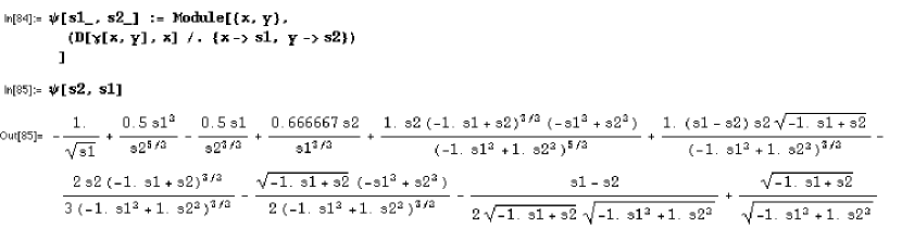
Figure 4: Ductility Sensitivity Definition.

Figure 5: Ductile Sensitivity.

III System Energy

As a digital system approaches the edges of it operating tolerance the energy required to maintain the performance increases as shown in Figure 6. Consider quality of service on a router in a communications network. The energy required to forward a packet is routinely modeled as directly proportional to the length of the packet. As the load increases, input queues begin to fill to capacity and packets are dropped because computational energy is not sufficient to keep up with the load. In this case, performance is the probability of not dropping a packet and energy is the processing power which is directly proportional to the packet service rate, $\mu$. In an M/M/1 queue, a direct relation between performance and energy is shown in Equation 4 where $n$ is the expected queue size, $N$ is the maximum queue capacity and $\rho={\lambda\over\mu}$. The result is graphed in Figure 7.

$$P[n<N]=\sum_{0}^{N-1}\rho^{n}(1-\rho)$$ (4)

Figure 6: System Performance and Energy.

Figure 7: Performance and Energy.

IV Brittle Sub-Components

Consider a system whose sub-components exhibit various degrees of ductility as defined above. Just as adding impurities to a pure metal causes it to become stronger but more brittle, the addition of more efficient but also more sensitive components to a system causes the system to increase performance within its operating range, but become less ductile. How do the effects of ductility propagate among the sub-components to influence the ductility of the entire system? Assume the performance response curve is known for each sub-component and that the output from one component feeds into the input of the next component as shown in Figure 8. Assume that the sub-component output performance cannot be better than any of its inputs. Then the performance curve for the output of each sub-component is the minimum of the input sub-component performance curve and the current component performance curve.

Figure 8: Brittle Subsystem Components.

The hardness component of the brittleness enhances the performance when values are within tolerance and low ductility degrades the performance when values are out of tolerance. The amount of degradation depends on the amount by which the tolerance was exceeded. This is illustrated in Figure 9 and is stated in Equation 5, where $b$ is the brittleness, $P_{in}$ is the input performance, $T$ is the set of in-tolerance values, $x$ is a state parameter, $E[]$ is the expected value, and $P_{out}$ is the output performance. The result of Equation 5 is plotted in Figure 10.

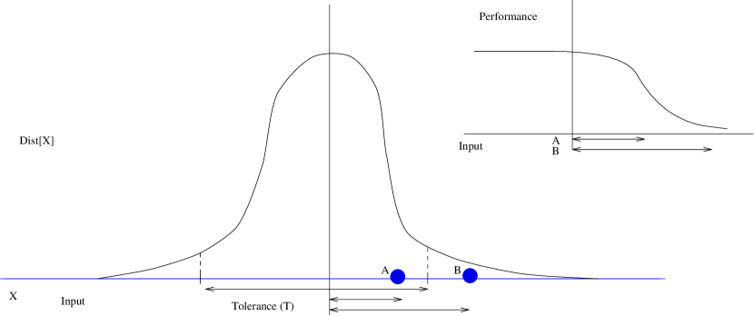
Figure 9: Distribution and Performance.

$$P_{out}=(P_{in}+P_{in}b)Prob[x\in T]+(P_{in}-P_{in}bE[x-max[T]])Prob[x\notin T]$$ (5)

Figure 10: Analytical Brittle Subcomponent Result.

As $b$ decreases in a non-brittle system, $T$ increases. It is this relationship between $b$ and $T$ which is the principal focus of brittle systems analysis. Assume the simple case of a normally distributed performance distribution, then Equation 6 shows how Equation 5 can be refined. $N(\eta,\sigma)$ is a normal distribution with an average of $\eta$ and variance of $\sigma$ and $R.V._{N(\eta,\sigma)}$ is a random variable with distribution $N(\eta,\sigma)$.

$$P_{out}=(P_{i}n+P_{in}b)Prob[R.V._{N(\eta,\sigma)}\leq T]+(P_{i}n-b\eta)1.0-Prob[R.V._{N(\eta,\sigma)}\leq T]$$ (6)

As $b$ decreases we assume that the system is non-brittle so that $T$ increases. Assume that $b$ is linear, then $T$ increases as shown in Figure 11 and Equation 7.

Figure 11: Relationship Between $b$ and $T$.

$$T=p_{x}+{1\over b}p_{y}$$ (7)

A BONeS model has been developed to examine brittle sub-components as shown in Figure 12 which models Figure 8. A BONeS data structure contains the performance or quality of the input to a component. A normal random number generator produces a value with a specified mean and variance, in this case 10.0 and 3.0 respectively. The difference between the random number and the upper limit (11.0) is computed. If the normal random number is greater than the upper limit, then the performance value of the input data structure is reduced by the brittleness multiplied by the amount by which the tolerance was exceeded. If the normal random number is within tolerance then the input data structure is increased by an amount proportional to the brittleness.

Figure 12: BONeS Model.

The results are shown in Figure 13 for the normal random number values, the upper limit, and the system performance as a function of the consecutive order in which each of the values were sampled. The brittleness is varied from zero to 0.8 and the results are averaged. Clearly the performance degrades when the normal values exceed the upper limit. Figure 14 shows the performance results for the sub-components and the entire system from Figure 12. Components 1 and 3 generate data structures with a performance value of one. An intermediate component, Component 2, has a brittleness which varies from zero to 0.8. The final output component, Component 4, has a brittleness of 0.3. The analytical results from Figure 10 and the simulated system performance curve from Figure 14 are in close agreement. Although Component 2 performance improves when the brittleness is between 0.2 and 0.5, Component 4, which is the system performance, declines. This is because Component 4 performance depends on the minimum performance input which comes from Component 3, an initial input component that always generates a performance of one.

Figure 13: System Performance.

Figure 14: Performance Curve.

If the ductility of sub-components can be controlled, how should the brittleness be adjusted among the sub-components? One line of reasoning yields the result that in systems run near the maximum operating tolerance, better performance will be achieved with highly brittle components placed near the outputs of the system. This is because there is then less chance for the highly brittle components to effect the other sub-components. The next simulation, shown in Figure 15 examines this question. The brittleness of the first component is varied from zero to one and the second component remains at a brittleness of 0.5. The results are shown in Figure 16. The results are also shown in the same figure for the first component brittleness of 0.5 and the second component brittleness varying from zero to one. Figure 16 indicates that the best performance curve results when the more highly brittle component is the last component in the chain.

Figure 15: Brittleness Location Experiment.

Figure 16: Brittleness Location Results.

V An Example of Ductility in a Communications Network

The following applications which exhibit brittle behavior have been chosen as simple examples so that the ideas presented in this work, rather than the details of the applications, can be investigated. These examples will be examined in more detail as this work progresses.

V-A Adaptive Multimedia

Current network applications, especially multimedia applications, have performance which degrades rapidly after bandwidth is reduced beyond a certain point. In [Lee] it is suggested that if applications can be developed which degrade gracefully with respect to loss in bandwidth as shown in Figure 17, then the network can be designed to maintain bandwidth within the required bounds on a best effort basis. A solution recommended in [Lee] is for the network to keep a certain amount of bandwidth in reserve. However, the more bandwidth kept in reserve, the less that remains to support the network as a whole. Thus the amount of reserve bandwidth is the greatest factor affecting ductility in this example. As the value of reserve bandwidth increases, the number of users which can be supported is reduced, but fewer calls in progress are disconnected.

Figure 17: Ductile Network Applications (Top Graph).

V-B Packet Recovery: Stop And Wait System

The second example is recovery from packet loss in an Automatic Repeat Request (ARQ) link shown in Figure 18. We consider two types of packets: packets with a large delay and packets which are lost. Setting a high time-out value results in better performance for packets which have a high ratio of delay to loss, but degrades rapidly as the ratio approaches zero.

Figure 18: Delay, Probability of Error, and Timeout in a Stop And Wait System.

V-C TDMA Reservation System

Figure 19 shows transmission rate versus probability of transmission for two values of retransmission. The lower valued setting for retransmission has higher performance, however, the higher valued retransmission setting is slightly more robust around a probability of 0.013.

Figure 19: TDMA Probability of Transmission and Transmission Rate.

V-D Mobile Cellular Telephone System

Figure 20 shows grade of service versus channels per base station.

Figure 20: Grade of Service versus number of Channels per Base Station.

V-E Buffer Capacity

Another example of a brittle system involves choosing buffer capacity in a data communications system.

V-F Backlogged Packets in Slotted ALOHA

In Slotted ALOHA, data packet transmission occurs using equal sized packets within equally divided time slots. If two or more users transmit within a given time slot, a collision occurs; the packet will be retransmitted in a following time slot with a given probability. This example of a brittle system exhibits catastrophic behavior [Nelson:1987:SCT]. Let $p_{0}$ be the probability that a packet to be transmitted finds an empty cell, and $p_{1}$ be the probability that after a collision, the cell attempts retransmission. The design parameters are $p_{0}$ and $p_{1}$ and the number of packets waiting for retransmission is the state. A graph of $p_{0}$ and $p_{1}$ forms a cusp and all the classic symptoms of catastrophe are present, namely, bifurcation, sudden jumps, hysteresis, inaccessibility, and divergence.

V-G Variable Window Flow Control

Figure 21: Variable Window Throughput Comparison.

V-H Flow Control

Also in [Nelson:1987:SCT], it is suggested that flow control, shown in Figure 21, in a communications network exhibits not only brittle behavior, but catastrophic behavior. The specific model of flow control considered in [Nelson:1987:SCT] is to divide available buffer space into classes and allow packets which have passed through $i$ hops to occupy buffers assigned to class $i$.

VI Techniques for Handling Brittle Systems

There are a variety of techniques for controlling and enhancing the ductility of a system. The first is to assign values to design parameters which influence ductility in a static manner, that is before the system becomes operational. The next involves dynamically changing the ductility as the system operates. This would be analogous to a material which could automatically trade-off hardness for ductility whenever necessary in order to maximize its performance. The remaining techniques involve methods of attempting to avoid brittle fracture, by design or by rolling back from a fracture.

VI-A Ductility Setting of System Sub-Components

Now that ductility has been defined and the design parameters controlling ductility identified, a natural question to ask is how should the sub-component parameters be set. Within normal operation, the performance requirements must be met, and in addition we would like the system to be tough (robust) outside the normal operating range as well. Is there a benefit to how ductility is distributed among subsystem components? As an example, in network and transport level data communications systems, if the system is going to fail, it is beneficial for low level system components to fail early in the transmission process rather than transporting a packet close to its destination and finding that the entire packet/frame has to be retransmitted later. Thus, it would be better to set $X_{1}$, in Figure 8, so that sub-component $S1$, which performs its processing early, has a lower ductility than components later in the process.

A highly brittle component, as illustrated in Figure 22, would appear to have the characteristics of an on-off constant bit rate (on-off CBR) source. These types of sources have been used to model ATM [Prycker] traffic sources. Queue fill distribution has been analyzed in [Anick1982] for on-off CBR models. These results could be used in a buffer solution for such highly brittle components.

Figure 22: An On-Off Brittle Sub-Component.

VI-B Adaptation

As mentioned previously, there are two forms of strain, reversible and permanent. Reversible strain is called elastic strain and is characterized by Young’s modulus: the ratio of the stress over the strain. Permanent strain leaves the shape of a material permanently changed and is known as plastic strain. In brittle systems, an analog to plastic strain is adaptation. Once we know the parameters which affect ductility, that is, having determined $\psi$, the values of the parameters can be changed dynamically as stress causes the system to approach a brittle fracture.

VI-C Rollback

Another possibility is that once the system approaches a brittle fracture, the system has the capability to rollback to a safe state and choose another gradient which attempts to remain in a safe state of operation. Rollback techniques within a communications network environment have been described in [BushThesis].

Stephen F. Bush Stephen F. Bush is a Computer Scientist at General Electric Research and Development (GE CR & D) in Niskayuna, NY. Steve is currently the Principal Investigator for the DARPA funded Active Networks Project at GE. Before joining GE CR & D, Stephen was a researcher at the Information and Telecommunications Technologies Center (ITTC) at the University of Kansas where he contributed to the DARPA Rapidly Deployable Radio Networks Project. He received his B.S. in Electrical and Computer Engineering from Carnegie Mellon University and M.S. in Computer Science from Cleveland State University. He has worked many years for industry in the areas of computer integrated manufacturing and factory automation and control. Steve received the award of Achievement for Professional Initiative and Performance for his work as Technical Project Leader at GE Information Systems in the areas of network management and control while pursuing his Ph.D. at Case Western Reserve University. Steve completed his Ph.D. research at the University of Kansas where he received a Strobel Scholarship Award. He can be reached at bushsf@crd.ge.com and http://www.crd.ge.com/people/bush.