Active Virtual Network Management Protocol

Abstract

This paper introduces a novel algorithm, the Active Virtual Network Management Protocol (AVNMP), for predictive network management. It explains how the Active Virtual Network Management Protocol facilitates the management of an active network by allowing future predicted state information within an active network to be available to network management algorithms. This is accomplished by coupling ideas from optimistic discrete event simulation with active networking. The optimistic discrete event simulation method used is a form of self-adjusting Time Warp. It is self-adjusting because the system adjusts for predictions which are inaccurate beyond a given tolerance. The concept of a streptichron and autoanaplasis are introduced as mechanisms which take advantage of the enhanced flexibility and intelligence of active packets. Finally, it is demonstrated that the Active Virtual Network Management Protocol is a feasible concept.

1 . Network Management and Active Networks

The problem this paper addresses is the complexity of managing large and rapidly growing communication networks. Network management consists of a wide variety of responsibilities including configuration management, performance management, fault management, accounting management, and security management. A network management system must be able to monitor, control, and report upon the status of all of these areas. This is usually performed using a standards based management protocol such as the Common Management Information Protocol (CMIP) [5] or the Simple Network Management Protocol (SNMP) [9]. A goal of network management is to pro-actively detect problems in each of these areas. This means detecting such events as performance problems and faults before they occur. This is accomplished by the Active Virtual Network Management Protocol.

Active networks [11] are a relatively recent concept in communication networks. Active networks are capable of executing general purpose code within packets as the packets are transmitted through intermediate network nodes. A framework for supporting the execution of general purpose code within packets as they travel through a network is an on-going research effort. Thus active networks differ from today’s communications networks because active networks offer a computational service in addition to a data transport service. In current communication networks non-executable data is passively forwarded through the traditional communication layers; intermediate devices such as bridges and routers only access the data link or network headers of packets. In active networks, intermediate devices can execute generic code within active packets as they travel through the network. The ability for communication networks to perform such computation offers opportunities for great advantages in such areas as efficiency, rapid protocol development and deployment, and network flexibility. However, active networks also add additional complexity, particularly in network management and security. The goal of the Active Virtual Network Management Protocol is to use the advantages active networks provide in order to handle the additional complexity in network management.

The Active Virtual Network Management Protocol caches predicted values within a State Queue and makes them available to a standard network management interface such as the SNMP [9] as shown in Figure 1. Because time is appended to the Object Identifier, a series of Get-Next requests will return all the predicted cached values of a Management Information Base (MIB) object. Also note in Figure 1 that the SNMP agent has the capability to reside within a packet. Because it is an active network, packets are capable of issuing management requests and responding to such requests.

Figure 1: Obtaining a Future MIB Object Value.

The predictive capability provided by the Active Virtual Network Management Protocol facilitates the development of a variety of predictive applications from mobile wireless location management and network security to improved Quality of Service (QoS). Mobile systems, especially those using the Global Positioning System can predict their location. This information can be propagated through the system via the Active Virtual Network Management Protocol. An example of predictive mobile wireless location management is described in [4]. Because the mobile host’s location can be predicted, the setup information required for hand-off can be cached ahead of time providing dramatic increases in the speed of hand-off and thus improved QoS. In the area of network security, given a set of vulnerabilities within a communications network, the most probable path an attacker will follow can be determined. The Active Virtual Network Management Protocol can thus incorporate the effect of an attack in its prediction and the consequences of a real or anticipated attack can be propagated through the system before it occurs. In regards to Quality of Service, time sensitive applications require a predictable Quality of Service [1]. The offered load at the input to the network can be predicted and the Active Virtual Network Management Protocol will transparently propagate the predicted load through intermediate network devices. An example of using predictive load management is described in [3]. An example of a method for predicting network traffic based on Wavelets [8] shows promise and can be used to implement the Driving Process (DP) within the Active Virtual Network Management Protocol. The Active Virtual Network Management Protocol driving process is described in Section 2.1.

2 . Active Virtual Network Management Protocol Description

The Active Virtual Network Management Protocol algorithm encapsulates each Physical Process within a Logical Process as illustrated in Figure 2. A Physical Process is nothing more than an executing task implemented by program code. An example of a Physical Process in a mobile wireless environment is the Rapidly Deployable Radio Network [10] beam table computation task. The beam table computation task generates a table of complex weights which controls the angle of radio beams based on position input. A Logical Process consists of the Physical Process and additional data structures and instructions which maintain message order and correct operation as the system executes ahead of real time. These structures are illustrated in detail in Figure 2. As an example, the beam table computation Physical Process is encapsulated in a Logical Process which maintains generated beam tables in its State Queue and handles rollback due to out-of-order input messages or out-of-tolerance real messages as explained in Section 2.2. A Logical Process contains a Receive Queue (QR), Send Queue (QS), and State Queue (SQ) as shown in Figure 2. The simulation component and simulation cache on the left side of Figure 2 represent the execution and state based upon virtual messages. The real time component and cache represent the execution and state based upon real messages. The Receive Queue maintains newly arriving messages in order by their Receive Time (TR). The Send Queue maintains copies of previously sent messages in order of their send times. The state of a Logical Process is periodically saved in the State Queue. The Logical Process also contains its notion of time known as Local Virtual Time (LVT) and a Tolerance ($\Theta$). The tolerance is the allowable deviation between actual and predicted values of incoming messages. For example, when a real message enters the beam table computation Logical Process the position in the message value is compared with the position which had been cached in the State Queue of the Logical Process. If these values are out of tolerance, then corrective action is taken in the form of a rollback as explained in Section 2.2.

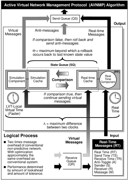
Figure 2: The AVNMP Logical Process.

The Active Virtual Network Management Protocol Logical Process has the contents shown in Table 1, the message fields are shown in Table 2, and the message types are listed in Table 3 where $t$ is the real time at the receiving Logical Process. Active Virtual Network Management Protocol messages contain the Send Time (TS), Receive Time (TR), Anti-toggle (A) and the actual message value itself (M). The Receive Time (TR) is the time this message is predicted to be valid at the destination Logical Process. It is not the link transfer time from source to destination Logical Process. The Send Time (TS) is the time this message was sent by the originating Logical Process. The “A” field is the anti-toggle and is used for creating an anti-message to remove the effects of false messages as described later. A message also contains a field for current Real Time (RT). This is used to differentiate a real message from a virtual message. A message which is generated and time-stamped with the current time is called a real message. Messages which contain future event information and are time-stamped with a time greater than current time are called virtual messages. If a message arrives at a Logical Process out of order or with invalid information, it is called a false message. A false message will cause a Logical Process to rollback.

Structure	Description
Receive Queue (QR)	Messages ordered
	by receive time (TR)
Send Queue (QS)	Messages ordered
	by send time (TS)
Local Virtual
Time (LVT)	$LVT=\inf RQ$
State Queue (SQ)	States are periodically saved
Sliding Lookahead
Window	$SLW=(t,t+\Lambda$]
Tolerance ($\Theta$)	Allowable deviation

Table 1: Active Virtual Network Management Protocol Logical Process Structures.

Field	Description
Send Time (TS)	LVT of sending process
	when message is sent
Receive Time (TR)	Scheduled time message
	is to be received
Anti-toggle (A)	Identifies message as
	normal or anti-message
Message (M)	Contents of the message
Real Time (RT)	GPS time message originated

Table 2: Active Virtual Network Management Protocol Message Fields.

Virtual Message	$RT>t$
Real Message	$RT\leq t$

Table 3: Active Virtual Network Management Protocol Message Types.

2.1 . Driving Process

The Active Virtual Network Management Protocol algorithm requires a Driving Process (DP) to predict future events and inject them into the system. The driving process acts as a source of virtual messages for the Active Virtual Network Management Protocol system. Virtual messages are injected at a rate of $\lambda_{vm}$ messages per unit time and each virtual message has a lookahead of $\Delta_{vm}$ time units. Logical Processes react to virtual messages. For example, in the case of mobile wireless networking, the Global Positioning System receiver process runs in real-time providing current time and location information and has been modified to inject future predicted time and location messages as well. Figure 3 shows an example how an active network would appear with Logical Processes and Driving Processes deployed. Notice that the driving processes define the scope of the system, that is, the degree to which the system is predictable. For example, if only a particular route is of interest for load prediction purposes, then driving processes may be sent only to adjacent tributary nodes of the path. One of the objectives of this research is to enable the logical and driving processes to automatically and dynamically locate themselves in optimal positions within the network.

Figure 3: Driving and Logical Processes within a Communications Network.

2.2 . Rollback

A rollback is triggered either by messages arriving out of order at the Receive Queue of a Logical Process or by a predicted value previously computed by this Logical Process which is beyond the allowable tolerance. These are known as false messages because both types of messages are sources of error. In either case, rollback is a mechanism by which a Logical Process returns to a known correct state. The rollback occurs just as in the original Time Warp algorithm [6]. There are three phases. In the first phase, the Logical Process state is restored to a virtual time strictly earlier than the Receive Time of the false message. In the second phase, anti-messages are sent to cancel the effects of any invalid messages which had been generated before the arrival of the false message. An anti-message contains exactly the same contents as the original message with the exception of an anti-toggle bit which is set. When the anti-message and original message meet, they are both annihilated. The final phase consists of executing the Logical Process forward in virtual time from its rollback state to the virtual time the false message arrived. No messages are canceled or sent between the virtual time to which the Logical Process rolled back and the virtual time of the false message. Because these messages are correct, there is no need to cancel or re-send them. This increases performance and it prevents additional rollbacks. Note that another false message or anti-message may arrive before this final phase has completed without causing problems.

3 . Streptichrons

In the Active Virtual Network Management Protocol architecture described thus far, there is a one-to-one correspondence between virtual messages and real messages. While this correspondence works well for adding prediction to protocols using a relatively small portion of the total bandwidth, it would clearly be beneficial to reduce the message load, especially when attempting to add prediction of the bandwidth itself. There are more compact forms of representing future behavior within an active packet besides a virtual message. For relatively simple and easily modeled systems, only the model parameters need be sent and used as input to the logical process on the appropriate intermediate device. Note that this assumes that the intermediate network device’s Logical Process is simulating the device operation and contains the appropriate model. However, because the payload of a virtual message is exactly the same as a real message, the payload of the virtual message can be passed to the actual device and the result from the actual device is intercepted and cached. In this case, the Logical Process is a thin layer of code between the actual device and virtual messages primarily handling rollback. An entire executable load model can be included within an active packet generated by the Driving Process and executed by the Logical Process. When the active packet reaches the target intermediate device, the load model provides virtual input messages to the Logical Process and the payload of the virtual message passed to the actual device as previously described. A $\overbrace{\mbox{Strepti}}^{bend}\overbrace{\mbox{chron}}^{time}$ is an active packet facilitating prediction as shown in Definition 1 which implements any of the above mechanisms.

$$\mbox{Streptichron}\stackrel{{\scriptstyle\rm\Delta}}{{=}}\left\{\begin{tabular}[l]{l}Input Model (Monte-Carlo) Model\\ Model Parameters (Self Adjusting)\\ Virtual Message (Self Adjusting)\end{tabular}\right.$$ (1)

4 . Autoanaplasis

$\overbrace{\mbox{Auto}}^{self}\overbrace{\mbox{anaplasis}}^{adjusting}$ is the self-adjusting characteristic of streptichrons. One of the virtues of the Active Virtual Network Management Protocol is the ability for the predictive system to adjust itself as it operates. This is accomplished in two ways. When real time reaches the time at which a predicted value had been cached, a comparison is made between the real value and the predicted value. If the values differ beyond a given tolerance, then the Logical Process rolls backward in time. Also, active packets which implement virtual messages adjust, or refine, their predicted values as they travel through the network. As a specific example consider a streptichron in the form of a simple virtual message which anticipates load as illustrated in Figure 4. Although the virtual message represents a message expected to exist in the future, the virtual message implementation exists in real time providing feedback to the predictive system. For example, as the virtual message travels from one intermediate node to another, the packet computes its transfer time and compares it with the predicted state at that time of the intermediate logical process causing a rollback if it is out of tolerance. Also, as the streptichron travels through the network and as real time approaches the streptichron’s Receive Time, the streptichron refines its predicted value.

Figure 4: A Streptichron Refines its Prediction as it Travels Through the Network.

5 . Class Hierarchy

The software architecture and state of the code under development are shown in Figure 5. Time is critical in the architecture of the Active Virtual Network Management Protocol system; thus, most classes are derived from class Date. Class AvnmpTime handles relative time operations. Class Gvt uses active the GvtPackets class to calculate global virtual time. Class AvnmpLP handles the bulk of the processing including rollback. Class Driver generates and injects real and virtual messages into the system. The PP class either simulates, or accesses, an actual device on behalf of the Logical Process. The PP class may not need to simulate the device because the payload of a virtual message is exactly the same as a real message; thus, the payload of the virtual message can be passed to the actual device and the result from the actual device is intercepted and cached. In this case, the Logical Process is a thin layer of code between the actual device accessed by the PP class. The GvtPacket class implements the Global Virtual Time packet which is exchanged by all logical and driving processes to determine global virtual time. The Streptichron class has been discussed in Section 4. Currently only the virtual message form of a streptichron has been implemented. The active packets have been implemented in both ANTS [11] and KU SmartPackets [7].

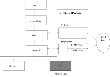
Figure 5: Active Virtual Network Management Protocol Class Hierarchy.

6 . Performance Analysis

This section analyzes the benefit of Active Virtual Network Management Protocol in terms of speedup based upon accurately predicting system behavior. There are many factors which influence speedup including out-of-order message probability, out-of-tolerance state value probability, rate of virtual messages entering the system, task execution time, task partitioning into Logical Processes, rollback overhead, prediction accuracy as a function of distance into the future which predictions are attempted, and the effect of parallelism and optimistic synchronization. All of these factors are considered in this section beginning with a direct analysis using the definitions from optimistic simulation.

The definition of Global Virtual Time (GVT) can be applied to determine the relationship among expected task execution time ($\tau_{task}$), the real time at which the state was cached ($t_{SQ}$), and real time ($t$). Consider the value ($V_{v}$) which is cached at real time $t_{SQ}$ in the State Queue (SQ) resulting from a particular predicted event. The state queue values may be repeatedly added and discarded as Active Virtual Network Management Protocol operation proceeds in the presence of rollback. As rollbacks occur, values for a particular predicted event may change, converging to the real value ($V_{r}$). For correct operation of Active Virtual Network Management Protocol, $V_{v}$ should approach $V_{r}$ as $t$ approaches $GVT(t_{1})$ where $GVT(t_{1})$ is the $GVT$ of the Active Virtual Network Management Protocol system at time $t_{1}$. Explicitly, this is for all $\epsilon>0$ there exists $\delta>0$ such that $|GVT(t_{1})-t|<\delta$ implies $|f(t)-f(GVT(t_{1}))|<\epsilon$ where $f(t)=V_{r}$ and $f(GVT(t_{1}))=V_{v}$. $f(t)$ is the prediction function of a driving process. The purpose and function of the driving process has been explained in Section 2. Because Active Virtual Network Management Protocol will always use the correct value when the predicted time ($\tau$) equals the current real time ($t$) and it is assumed that the predictions will become more accurate as the predicted time of the event approaches the current time, the reasonable assumption is made that $\lim_{\tau\rightarrow t}f(\tau)=V_{v}$. In order for the Active Virtual Network Management Protocol system to always look ahead, for all $t$ $GVT(t)\geq t$. This means that for all $n\in\{LPs\}$ and for all $t$ $LVT_{lp_{n}}(t)\geq t$ and $\min_{m\in\{M\}}\{m\}\geq t$ where $m$ is the receive time of a message, $M$ is the set of messages in the entire system and $LVT_{lp_{n}}$ is the Local Virtual Time of the $n^{th}$ Logical Process. In other words, the Local Virtual Time (LVT) of each Logical Process (LP) must be greater than or equal to real time and the smallest message Receive Time not yet processed must also be greater than or equal to real time. The smallest message Receive Time could cause a rollback to that time. This implies that for all $n,t$ $LVT_{dp_{n}}(t)\geq t$. In other words, this implies that the Local Virtual Time (LVT) of each driving process must be greater than or equal to real time. An out-of-order rollback occurs when $m<LVT(t)$. The largest saved state time such that $t_{SQ}<m$ is used to restore the state of the Logical Process, where $t_{SQ}$ is the real time the state was saved. Then the expected task execution time ($\tau_{task}$) can take no longer than $t_{SQ}-t$ to complete in order for $GVT$ to remain ahead of real time. Thus, a constraint between expected task execution time ($\tau_{task}$), state save time ($t_{SQ}$), and real time ($t$) has been defined. There are three possible cases to consider when determining the speedup of the Active Virtual Network Management Protocol over non-lookahead sequential execution. In this section we will determine the speedup given each of these cases and their respective probabilities. These cases are illustrated in Figures 6 through 8. The time that an event is predicted to occur and the result cached is labeled $t_{virtual\ event}$, the time a real event occurs is labeled $t_{real\ event}$, and the time a result for the real event is calculated is labeled $t_{no-avnmp}$. In the Active Virtual Network Management Protocol, the virtual event and its result can be cached before the real event as shown in Figure 6, between the real event but before the real event result is calculated shown in Figure 7, or after the real event result is calculated as shown in Figure 8. In each case, all events are considered relative to the occurrence of the real event. It is assumed that the real event occurs at time $t$. A random variable called the lookahead ($LA$) is defined as $LVT-t$. The virtual event occurs at time $t-LA$. Assume that the task which must be executed once the real event occurs takes $\tau_{task}$ time. Then without the Active Virtual Network Management Protocol the task is completed at time $t+\tau_{task}$.

Figure 6: Active Virtual Network Management Protocol Cached before Real Event.

Figure 7: Active Virtual Network Management Protocol Cached later than Real Event.

Figure 8: AVNMP Cached slower than Real Time.

The prediction rate of a Logical Process is the rate of change of the processes’ Local Virtual Time with respect to real time, thus $PR$ is the Active Virtual Network Management Protocol speedup. The prediction rate has been derived in [2] and is defined in Equation 6. $S_{parallel}$ is the speedup due to parallelism, $\Delta_{vm}$ is the lookahead per virtual message, $\lambda_{vm}$ is the rate at which virtual messages are injected by a driving process, $X$ and $Y$ are random variables representing the proportion of out-of-order and out-of-tolerance messages respectively, $\tau_{task}$ is the expected amount of time taken by the physical process to process an input message, and $\tau_{rb}$ is the expected time taken by a Logical Process to rollback. Equation 6 includes the time to predict an event and cache the result in the State Queue (SQ).

In [2] the expected value of $X$ has been determined based on the inherent synchronization of the Logical Process topology. It is shown in [2] that $X$ has an expected value which varies with the rate of hand-offs in the mobile wireless location management application. It is clear that the proportion of out-of-order messages is dependent on the Logical Process (LP) architecture and the partitioning of tasks into Logical Processes. Thus, it is difficult in an experimental implementation to vary $X$. It is easier to change the tolerance rather than change the Logical Process architecture to evaluate the performance of the Active Virtual Network Management Protocol. For these reasons, the analysis proceeds with $PR_{X,Y|X=E[X]}$. Since the prediction rate is the rate of change of Local Virtual Time with respect to time, the value of the Local Virtual Time is shown in Equation 6 where $C$ is an initial offset. This offset may occur because the Active Virtual Network Management Protocol may begin running $C$ time units before or after the real system. Replacing $LVT$ in the definition of $LA$ with the right side of Equation 6 yields the Equation for lookahead shown in Equation 4.

$$PR_{X,Y}=$$

$$\lambda_{vm}\left(\Delta_{vm}S_{parallel}-\tau_{task}-(\tau_{task}+\tau_{rb})X-(\Delta_{vm}S_{parallel}-{1\over\lambda_{vm}})Y\right)$$

$$LVT_{X,Y|X=E[X]}=$$

$$\lambda_{vm}(\Delta_{vm}S_{parallel}-\tau_{task}-(\tau_{task}+\tau_{rb})E[X]-$$

$$(\Delta_{vm}S_{parallel}-{1\over\lambda_{vm}})Y)t+C$$

$$LA_{X,Y|X=E[X]}=(LVT_{X,Y|X=E[X]}-1)t+C$$ (4)

The probability of the event in which the Active Virtual Network Management Protocol result is cached before the real event is defined in Equation 5. The probability of the event for which the Active Virtual Network Management Protocol result is cached after the real event but before the result would have been calculated in the non-Active Virtual Network Management Protocol system is defined in Equation 6. Finally, the probability of the event for which the Active Virtual Network Management Protocol result is cached after the result would have been calculated in a non-Active Virtual Network Management Protocol system is defined in Equation 7.

$$P_{cache}=P[LA_{X,Y|X=E[X]}>\tau_{task}]$$ (5)

$$P_{late}=P[0\leq LA_{X,Y|X=E[X]}\leq\tau_{task}]$$ (6)

$$P_{slow}=P[LA_{X,Y|X=E[X]}<0]$$ (7)

The goal of this analysis is to determine the effect of the proportion of out-of-tolerance messages ($Y$) on the speedup of a Active Virtual Network Management Protocol system. Hence we assume that the proportion $Y$ is a binomially distributed random variable with parameters $n$ and $p$ where $n$ is the total number of messages and $p$ is the probability of any single message being out of tolerance. It is helpful to simplify Equation 4 by using $\gamma_{1}$ and $\gamma_{2}$ as defined in Equations 9 and 10 in Equation 8.

$$LA_{X,Y|X=E[X]}=\gamma_{1}-\gamma_{2}Y$$ (8)

$$\gamma_{1}=(\lambda_{vm}\Delta_{vm}S_{parallel}-\lambda_{vm}\tau_{task}-$$ (9)

$$\lambda_{vm}(\tau_{rb}+\tau_{task})E[X])-1)t+C$$

$$\gamma_{2}=\lambda_{vm}(\Delta_{vm}S_{parallel}-{1\over\lambda_{vm}}+\tau_{rb})t$$ (10)

The early prediction probability as illustrated in Figure 6 is shown in Equation 11. The late prediction probability as illustrated in Figure 7 is shown in Equation 12. The probability for which Active Virtual Network Management Protocol falls behind real time as illustrated in Figure 8 is shown in Equation 13. The three cases for determining Active Virtual Network Management Protocol speedup are thus determined by the probability that $Y$ is greater or less than two thresholds.

$$P_{1}(t)=P_{{cache}\ {X,Y|X=E[X]}}=P\left[Y<{{\gamma_{1}-\tau_{task}}\over\gamma_{2}}\right]$$ (11)

$$P_{2}(t)=P_{{late}\ {X,Y|X=E[X]}}=P\left[{{\gamma_{1}-\tau_{task}}\over\gamma_{2}}\leq Y\leq{\gamma_{1}\over\gamma_{2}}\right]$$ (12)

$$P_{3}(t)=P_{{slow}\ {X,Y|X=E[X]}}=P\left[Y>{\gamma_{1}\over\gamma_{2}}\right]$$ (13)

The three probabilities in Equations 11 through 13 depend on ($Y$) and real time because the analysis assumes that the lookahead increases indefinitely which shifts the thresholds in such a manner as to increase Active Virtual Network Management Protocol performance as real time increases. However, in this analysis, it is assumed that a sliding lookahead window exists on each Logical Process to control the lookahead rate locally. The Active Virtual Network Management Protocol algorithm holds processing of virtual messages once the end of the Sliding Lookahead Window (SLW) is reached. The hold time occurs when $LA=\Lambda$ where $\Lambda$ is the length of the Sliding Lookahead Window. Once $\Lambda$ is reached, processing of virtual messages is discontinued until real-time reaches Local Virtual Time. The lookahead versus real time including the effect of the Sliding Lookahead Window is shown in Figure 9. The dashed arrow represents the lookahead which increases at rate $PR$. The solid line returning to zero is lookahead as the Logical Process delays. Because the curve in Figure 9 from $0$ to $t_{L}$ repeats indefinitely, only the area from $0$ to $t_{L}$ need be considered. For each $P_{i}(t)$ $i=1,2,3$, the time average over the lookahead time ($t_{L}$) is shown by the integral in Equation 14.

$$P_{X,Y|X=E[X]}={1\over t_{L}}\int_{0}^{t_{L}}P_{i}(t)dt$$ (14)

Figure 9: Lookahead with a Sliding Lookahead Window.

The probability of each of the events shown in Figures 6 through 8 is multiplied by the speedup for each event in order to derive the average speedup. For the case shown in Figure 6, the speedup ($C_{r}$) is provided by the time to read the cache over directly computing the result. For the remaining cases the speedup is $PR_{X,Y|X=E[X]}$ which has been defined as ${LVT_{X,Y|X=E[X]}\over t}$ as shown in Equation 6. The analytical results for speedup are graphed in Figure 10. A high probability of out-of-tolerance rollback in Figure 10 results in a speedup of less than one. Real messages are always processed when they arrive at an Logical Process. Thus, no matter how late Active Virtual Network Management Protocol results are, the system will continue to run near real time. However, when Active Virtual Network Management Protocol results are very late due to a high proportion of out-of-tolerance messages, the Active Virtual Network Management Protocol system is slower than real time because out-of-tolerance rollback overhead processing occurs. Anti-messages must be sent to correct other Logical Processes which have processed messages which have now been found to be out of tolerance from the current Logical Process. This causes the speedup to be less than one when the out-of-tolerance probability is high. Thus, $PR_{X,Y|X=E[X]}<1$ for the “slow” case shown in Figure 8.

$$\eta\equiv$$

$$P_{{cache}\ {X|X=E[X]}}C_{r}+(P_{{late}\ {X|X=E[X]}}+P_{{slow}\ {X|X=E[X]}})PR_{X,Y|X=E[X]}$$

Figure 10: AVNMP Speedup.

Equation 6 shows the complete Active Virtual Network Management Protocol performance utility. The surface plot showing the utility of Active Virtual Network Management Protocol as a function of the proportion of out-of-tolerance messages is shown in Figure 11 where $\Phi_{s}$, $\Phi_{w}$, $\Phi_{b}$ are one. The parameters are chosen to accommodate the mobile wireless network application described in [2]. Virtual messages are injected by the Global Positioning System at a rate of 0.03 per millisecond ($\lambda_{vm}=0.03$) with a lookahead of 30.0 milliseconds ($\Delta_{vm}=30.0$). The expected time to create a beam table is 7.0 milliseconds ($\tau_{task}=7.0$). The expected rollback time is 1.0 milliseconds ($\tau_{rb}=1.0$) and the speedup in reading from cached results over computing the beam table is 100 ($C_{r}=100$). The y-axis is the relative marginal utility of speedup over reduction in bandwidth overhead $SB=\frac{\Phi_{s}}{\Phi_{b}}$. Thus if bandwidth reduction is much more important than speedup, the utility is low and the proportion of rollback messages would have to be kept below 0.3 in this case. However, if speedup is of higher priority relative to bandwidth, the proportion of out-of-tolerance rollback message values can be as high as 0.5. If the proportion of out-of-tolerance messages becomes too high, the utility becomes negative because prediction time begins to fall behind real time.

The effect of the proportion of out-of-order and out-of-tolerance messages on Active Virtual Network Management Protocol speedup is shown in Figure 12. This graph shows that out-of-tolerance rollbacks have a greater impact on speedup than out-of-order rollbacks. The reason for the greater impact of the proportion of out-of-tolerance messages is that rollbacks caused by such messages always cause a process to rollback to real time. An out-of-order rollback only requires the process to rollback to the previous saved state.

Figure 13 shows the effect of the proportion of virtual messages and expected lookahead per virtual message on speedup. This graph is interesting because it shows how the proportion of virtual messages injected into the Active Virtual Network Management Protocol system and the expected lookahead time of each message can affect the speedup. The real and virtual message rates are 0.1 messages per millisecond and the remaining parameters remain as previously stated.

$$U_{AVNMP} = \left(P_{{cache}\ {X|X=E[X]}}C_{r}+\right.$$

$$\left.(P_{{late}\ {X|X=E[X]}}+P_{{slow}\ {X|X=E[X]}})PR_{X,Y|X=E[X]}\right)\Phi_{s}-$$

$$P[|AC_{t}(\Lambda)|>\Theta]\Phi_{w}-$$

$$\left({\frac{\lambda_{v}}{\lambda_{rb}}+\lambda_{v}}\over\lambda_{r}\right)\Phi_{b}$$

Figure 11: Overhead versus Speedup as a Function of Probability of Rollback.

Figure 12: Effect of Non-Causality and Tolerance on Speedup.

Figure 13: Effect of Virtual Message Rate and Lookahead on Speedup.

7 . Summary

This paper has introduced a novel algorithm, Active Virtual Network Management Protocol (AVNMP), for predictive network management. It explained how the Active Virtual Network Management Protocol facilitates the management of an active network by allowing future predicted state information within an active network to be available to network management algorithms. This has been accomplished by coupling ideas from optimistic discrete event simulation with active networking. The optimistic discrete event simulation method used is a form of self-adjusting Time Warp. The concept of a streptichron and autoanaplasis have been introduced as mechanisms which take advantage of the enhanced flexibility and intelligence of active packets. Finally, it has been demonstrated that the Active Virtual Network Management Protocol is a feasible concept.

Future work on the Active Virtual Network Management Protocol will focus on dynamic message reprioritization such that both real and virtual messages are processed with optimal priority as well as automatic dynamic deployment of the Active Virtual Network Management Protocol logical and driving processes within a network. Work will also continue on finding synergies between the self-adjusting Time Warp algorithm and active networks in order to optimize the Active Virtual Network Management Protocol.

References

- [1] R. Braden, D. Clark, and S. Shenker. Integrated services in the internet architecture: an overview, June 1994. RFC #1633.
- [2] S. F. Bush. The Design and Analysis of Virtual Network Configuration for a Wireless Mobile ATM Network. PhD thesis, University of Kansas, Aug. 1997.
- [3] S. F. Bush, V. S. Frost, and J. B. Evans. Network Management of Predictive Mobile Networks. In IEEE Symposium on Planning and Design of Broadband Networks, October 1996. Session 8, Montebello, Quebec, Canada.
- [4] S. F. Bush, S. Jagannath, J. B. Evans, V. Frost, G. Minden, and K. S. Shanmugan. A Control and Management Network for Wireless ATM Systems. ACM-Baltzer Wireless Networks (WINET), 3:267,283, 1997. URL: http://www.ittc.ukans.edu/sbush.
- [5] ISO. Open Systems Interconnection - Management Protocol Specification - Part 2: Common Management Information Protocol.
- [6] D. R. Jefferson and H. A. Sowizral. Fast Concurrent Simulation Using The Time Warp Mechanism, Part I: Local Control. Technical Report TR-83-204, The Rand Corporation, 1982.
- [7] A. B. Kulkarni, G. J. Minden, R. Hill, Y. Wijata, S. Sheth, H. Pindi, F. Wahhab, A. Gopinath, and A. Nagarajan. Implementation of a Prototype Active Network. In OPENARCH ’98, 1998.
- [8] S. Ma and C. Ji. Wavelet models for video time-series. In M. I. Jordan, M. J. Kearns, and S. A. Solla, editors, Advances in Neural Information Processing Systems, volume 10. The MIT Press, 1998.
- [9] M. T. Rose. The Simple Book, An Introduction to the Management of TCP/IP Based Internets. Prentice Hall, 1991.
- [10] R. Sanchez, J. Evans, G. Minden, and V. S. F. K. S. Shanmugan. RDRN: A Rapidly Deployable Radio Network - Implementation and Experience. In ICUPC ’98, 1998.
- [11] D. L. Tennenhouse, J. M. Smith, W. D. Sincoskie, D. J. Wetherall, and G. J. Minden. A survey of active network research. IEEE Communications Magazine, 35(1):80–86, Jan. 1997.