Algorithms of Two-Level Parallelization for DSMC of Unsteady Flows in Molecular Gasdynamics

A.V. Bogdanov, N.Yu. Bykov, I.A. Grishin, Gr.O. Khanlarov, G.A. Lukianov and V.V. Zakharov

submitted for publication to the conference HPCN’99

Abstract
The general scheme of two-level parallelization (TLP) for direct simulation Monte Carlo of unsteady gas flows on shared memory multiprocessor computers has been described. The high efficient algorithm of parallel independent runs is used on the first level. The data parallelization is employed for the second one.

Two versions of TLP algorithm are elaborated with static and dynamic load balancing. The method of dynamic processor reallocation is used for dynamic load balancing.

Two gasdynamic unsteady problems were used to study speedup and efficiency of the algorithms. The conditions of efficient application field for algorithms have been determined.

©Institute for High Performance Computing and Data Bases

1 Introduction

1.1 Direct Simulation Monte Carlo Method and Sequential
Algorithm in Unsteady Molecular Gasdynamics

The Direct Simulation Monte Carlo (DSMC) is the simulation of real gas flows with various physical processes by means of huge number of modeling particles [1], each of which is a typical representative of great number of real gas particles (molecules, atoms, etc.). The DSMC method conditionally divides the continuous process of particles movement and collisions into two consecutive stages (motion and collision process) at each time step $\Delta t$. The particle parameters (coordinates, velocity) are stored in the computer’s memory. To get information about the flow field the computational domain has to be divided into cells. The results of simulation are averaged particles parameters in cells.

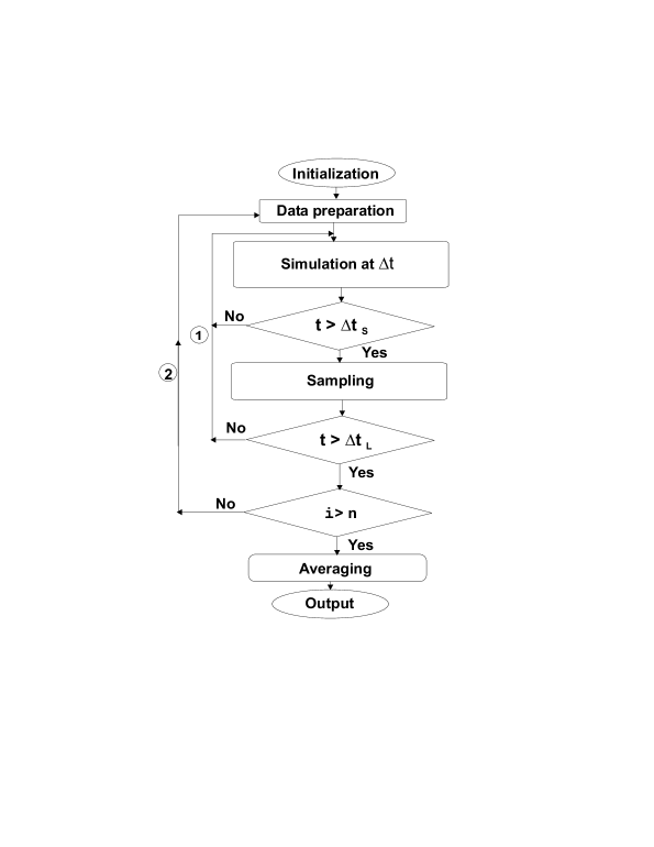
Figure 1: General flowchart of sequential algorithm for DSMC of unsteady flows. $\Delta t$ — time step, $\Delta t_{s}$ — interval between samples, $\Delta t_{L}$ — total time of a single run, $t$ — current time, $n$ — number of runs, $i$ — iteration number.

The finite memory size and computer performance make restrictions to the total number of modeling particles and cells. Macroscopic gas parameters determined by particles parameters in cells at the current time step are the result of simulation. Fluctuations of averaged gas parameters at single time step can be rather high owing to relatively small number of particles in cells. So, when solving steady gasdynamic problems, we have to increase the time interval of averaging (the sample size) after steady state is achieved in order to reduce statistical error down to the required level. The averaging time step $\Delta t_{av}$ has to be much greater than the time step $\Delta t$ ($\Delta t_{av}\gg\Delta t$).

For DSMC of unsteady flows the value of averaging time step $\Delta t_{av}$ for a given problem and at the current time $t$ has to meet the following requirement: $\Delta t_{av}\ll\min t_{H}(x,y,z,t)$, where $t_{H}$ — is the characteristic time of flow parameters variation. The choice of the value of $t_{H}$ is determined by particular problem [4, 14]. In order to meet the condition for the averaging interval we have to carry out enough number of statistically independent calculations (runs) $n$ to get the required sample size. This leads to the increase of the total calculation time which is proportional to $n$ in the case of sequential DSMC algorithm.

The general flowchart of classic sequential algorithm [1] is depicted in the fig. 1. The algorithm of DSMC of unsteady flows consists of two basic loops. In the first (inner) loop the single run of unsteady process is executed. First, we generate particles at input boundaries of the domain (subroutine Generation). Then we carry out simulation of particle movement, surface interaction (subroutine Motion) and collision process (subroutine Interaction) for determined number of time steps $\Delta t$. The sampling (subroutine Sampling) of flow macroparameters in cells is carried out at a given moment of unsteady process. The inner loop itself is divided into two successive steps. At the first step we sequentially carry out simulation for each of $N_{p}$ particles independently. A special readdressing array is formed – subroutines Enumeration, Indexing – (it determines the mutual correspondence of particles and cells) after the first step. We have to know the location of all particles in order to fill that array. At the second step we carry out the simulation for each of $N_{c}$ cells independently. For $t>\Delta t_{s}$ we accumulate statistical data of flow parameters in cells.

The second (outer) loop repeats unsteady runs $n$ times to get the desired sample size. Each run is executed independently from the previous ones. To make separate unsteady runs independent we have to shift random number generator (RNG).

For each unsteady run three basic arrays (P, LCR, C) are required. The array P is used for storing information about particles. The array LCR is the readdressing array. The dimensions of these arrays are proportional to the total number of particles. The array C stores information about cells and macroparameters. The dimension of this array is proportional to the total number of cells of a computational grid. The DSMC method requires several additional arrays which reserve much smaller memory size. The particles which abandon the domain are removed from the array P, whereas the new generated particles are inserted into the one. Since the particles move from one cell to another we have to rearrange the array LCR and update the array C. These procedures are performed at each time step $\Delta t$.

1.2 Parallelization methods for DSMC of gas flows

The feasibility of parallelization and the efficiency of parallel algorithms are determined both by the structure of modeling process and by the architecture and characteristics of a computer (number of processors, memory size, etc.).

The development of any parallel algorithm starts with the decomposition of a general problem. The whole task is divided into a series of independent or slightly dependent sub-tasks which are solved parallel. For direct simulation of gas flows there are different decomposition strategies depending on goals of modeling and flow nature. The development of parallel algorithms for DSMC started not long ago (about 10 years ago). At the present time the common classification of principal types of parallel algorithms has not been formed yet. However, one can point out several approaches to parallelize the DSMC, the efficiency of which is proved by the practice of their usage. Let us conditionally single out four types of parallel algorithms of DSMC.

The first type is the parallelization by coarse-grained independent sub-tasks. This method has been realized in [2]–[4] for parallelization of DSMC of unsteady problems. The algorithm consists in the reiteration of statistically independent modeling procedures (runs) of a given flow on several processors.

The second type is the spatial decomposition of a computational domain. The calculation in each of regions are single sub-tasks which are solved parallel. Each processor performs calculations for particles and cells in its own region. The transfer of particles accompanies with data exchange between processors. Therefore, these sub-tasks are not independent.

This method of parallelization is the most widespread at the present for parallel DSMC of both steady and unsteady flows [5]–[11]. The main advantage of this approach is the reduction of memory size required by each processor. This method can be carried out on computers with both local and shared memory. The method has drawback for increasing number of processors: the increase of the number of connections between regions and the increase of relative amount of data to exchange between regions. The essential condition of high efficiency of this method is the ensuring of uniform load balancing and minimization of data exchange. One can use static and dynamic load balancing to make good load balancing. The modern parallel algorithms of this type usually employ dynamic load balancing.

The third type is the algorithmic decomposition. This type of parallel algorithms consists in the execution of different parts of the same procedures on different processors. For realization of these algorithms it is necessary to use a computer with architecture which is adequate to a given algorithm. The examples of this type of algorithm is the data parallelization [12, 13].

The fourth type is the combined decomposition which includes all types considered precedingly. The decomposition of computational domain with data parallelization are carried out in [12]. In this paper we shall consider two-level algorithms which include methods of first and third type.

1.3 Algorithm of Parallel Statistically
Independent Runs (PSIR) [4]

The statistical independence of single runs make it possible to execute them parallel. The general flowchart of the PSIR algorithm is depicted in the fig. 2. The implementation of this approach on a multiprocessor computer leads to the decrease of the number of iterations of the outer loop for every single processor ($n/p$ — the number of iterations for the $p$-processor computer). The data exchange between processors goes after all calculation are finished. Only one processor sequentially analyzes the results after data exchange. The range of efficient application field for this algorithm is $p\leq n$. The value of $n$ has to be multiply by $p$ to get optimal speedup and efficiency.

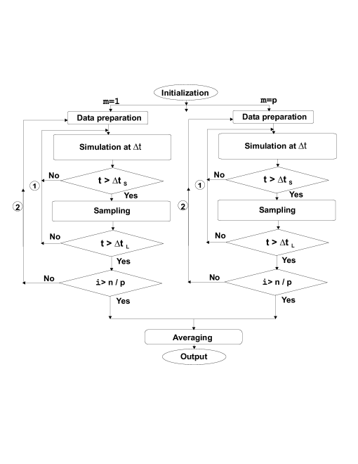
Figure 2: General flowchart of PSIR algorithm; $m$ — processor ID, $p$ — number of processors.

All arrays (P, LCR, C, etc.) are stored locally for each run. This algorithm can be realized on computers with any type of memory (shared or local). The message passing is used to perform data exchange on computers with local memory. The scheme of memory usage is presented in the fig. 3. The required memory size for this algorithm is proportional to $p$.

Figure 3: Scheme of memory usage for PSIR algorithm (the case of three processors).

The speedup $S_{p}$ and the efficiency $E_{p}$ of parallel algorithm with a parallel fraction of computational work $\alpha$ for the computer with $p$ processors are as follows [15]:

$$S_{p}(p,\alpha)=\frac{T_{1}}{T_{p}},$$ (1)

$$E_{p}(p,\alpha)=\frac{S_{p}}{p},$$ (2)

where $T_{1}$ — the execution time of the sequential algorithm, $T_{p}$ — the execution time of a given parallel algorithm on the computer with $p$ processors ($p$ — number of reserved processors). In this paper we use a model of computational process which assumes that there is some parallel fraction $\alpha$ of total calculations and sequential fraction $(1-\alpha)$. The parallel and sequential calculations are not coincided.

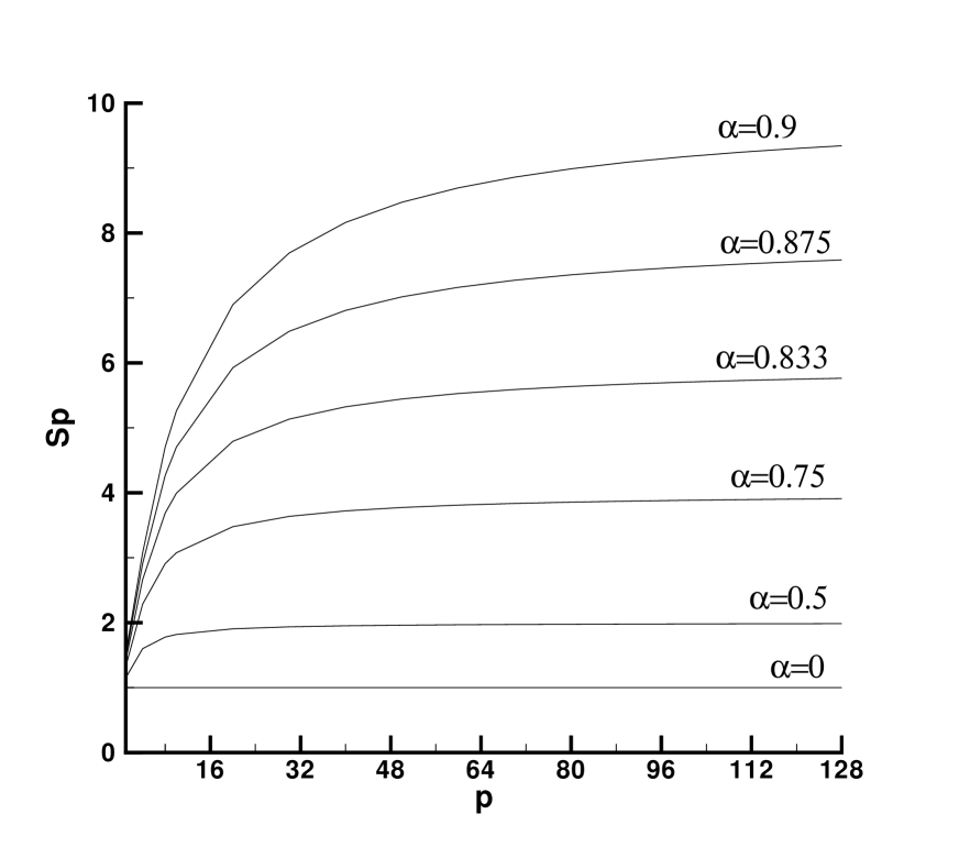
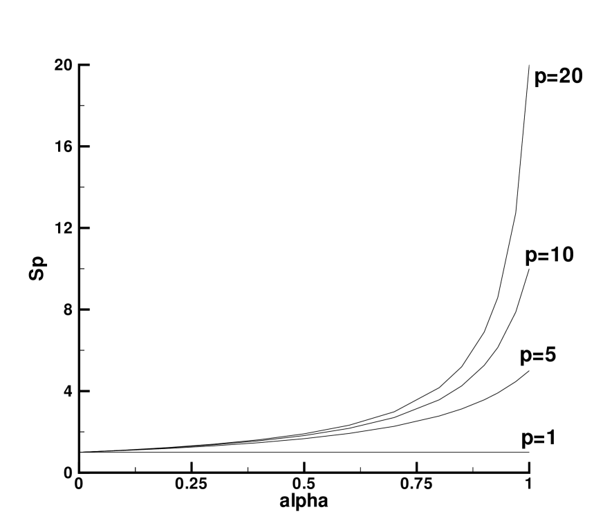
Figure 4: Speedup $S_{p}$ as a function of number of processors $p$ for various parallel fractions $\alpha$ (left), speedup $S_{p}$ as a function of parallel fraction $\alpha$ for various number of processors $p$ (right).

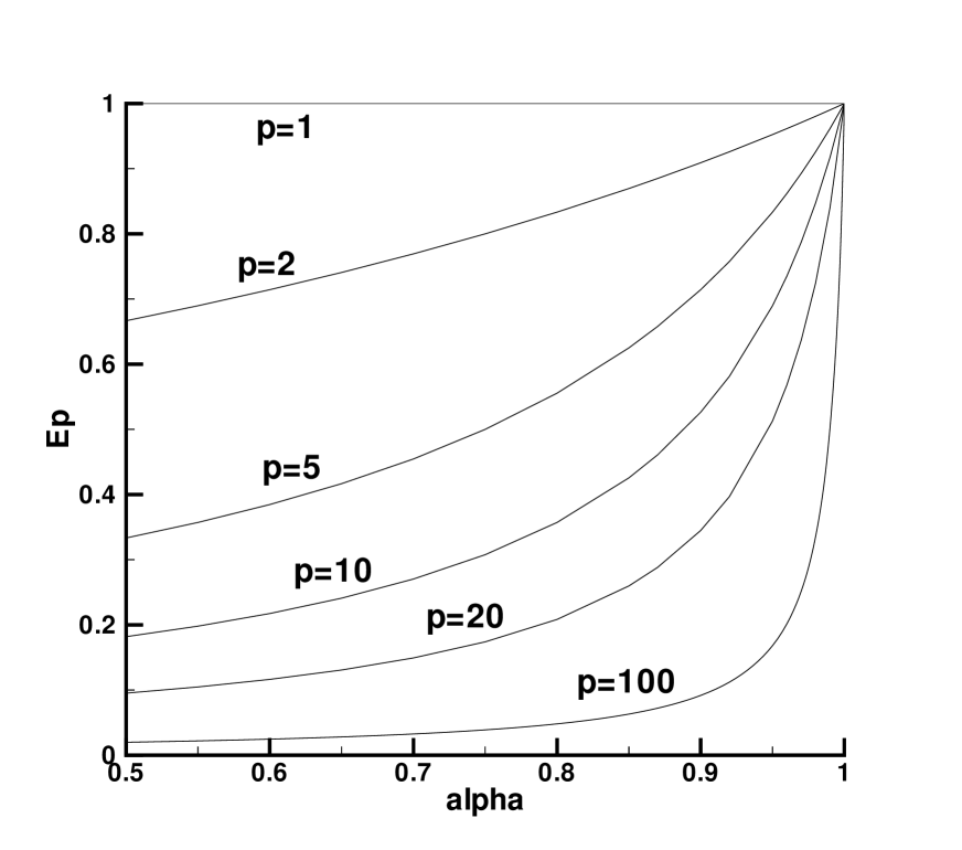
Figure 5: Efficiency $E_{p}$ as a function of parallel fraction $\alpha$ for various number of processors $p$

The value of $T_{p}$ is given by

$$T_{p}=[(1-\alpha)+\alpha/p]T_{1}.$$ (3)

To get the value of $\alpha$ one may use a profiler. The final formulas for $S_{p}$ and $E_{p}$ are as follows:

$$S_{p}(p,\alpha)=\frac{p}{p-\alpha(p-1)},$$ (4)

$$E_{p}(p,\alpha)=\frac{1}{(1-\alpha)p+\alpha}.$$ (5)

The formula (4) presents a simple and general function, called the Amdahl law. According to this law, the speedup upper limit at $p\rightarrow\infty$ for an algorithm, which has two non-coinciding parallel and sequential parts, is as follows:

$$S_{p}(p,\alpha)\leq\frac{1}{1-\alpha}.$$ (6)

To speed up calculations we have to speed up parallel computations, however, the remaining sequential part slows down the overall computing process to more and more extent. Even small sequential fraction may reduce greatly the overall performance.

The figure 4 shows the speedup $S_{p}$ as a function of number of processors $p$ and parallel fraction $\alpha$. The efficiency $E_{p}$ as a functon of $\alpha$ is shown in the fig. 5. Sequential computations affected speedup and efficiency particularly in the region $\alpha>0.9$. Therefore, even small decrease of sequential computations in algorithms with high parallel fraction makes speedup and efficiency abruptly increase (at relatively high $p$).

The PSIR algorithm is coarse-grained and has high efficiency and great degree of parallelism comparing to any other parallel algorithm of DSMC of unsteady flows for the number of processor $p\leq n$. The maximum value of speedup for this algorithm can be obtained at $p=n$. The potential of speedup which gives the computer is surplus for $p>n$. Thus, the PSIR algorithm for DSMC of unsteady flows has the following range of efficient usage: $n\gg 1$ and $n\geq p$. The value of parallel fraction $\alpha$ can be very high (up to $0.99\div 0.999$) for typical problems of molecular gasdynamics [4]. The corresponding speedup is $100\div 1000$. To get the efficiency $E_{p}\geq 0.5$ at $n=100\div 1000$ it is necessary to have $p=100\div 1000$ respectively.

1.4 Data Parallelization (DP) of DSMC [13]

The computing time of each DSMC problem is determined by the inner loop (1) time. The duration of this loop depends on the number of particles in the

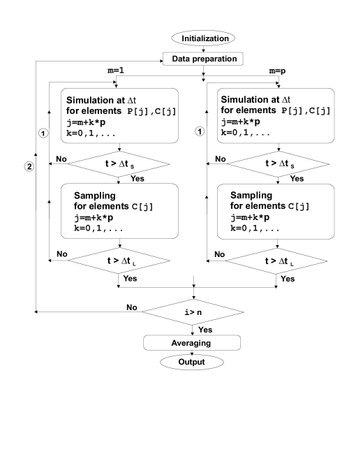
Figure 6: General flowchart of DP algorithm; $j$ — index of data element

domain and the number of cells. It was stated above that the inner loop consists of two consecutive stages. The data inside each stage are independent. The elements P[k] are processed at the first stage, whereas the elements C[k] — at the second one (the elements of arrays P and C are mutually independent). Since the operations on each of these elements are independent it is possible to process them parallel. Each processor takes elements from particle array P and cell array C according to its unique ID-number, i.e. the m-th processor takes the $m$-th, ($m+p$)-th, ($m+2p$)-th, etc. elements, where “$m$” is the processor ID-number. This rule of particle selection provides good load balancing because various particles require different time to process and they are located randomly in the array P .

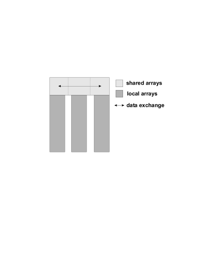
Figure 7: Scheme of memory usage for DP algorithm (three processors)

The synchronization of processors is performed before the next loop iteration starts. Before the second stage begins it is necessary to fill the readdressing array LCR. The complete information about the array P is required for readdresing procedure. This task can not be parallelized, so it is performed by one processor. There are two synchronization points before the readdressing and after the one. The reduction of the computational time is due to the decrease of the amount of data which has to be processed by each processor ($N_{p}/p$ and $N_{c}/p$ instead of $N_{p}$ and $N_{c}$). After the inner loop is passed the processors also need to get synchronized. The figure 6 shows the general flowchart of DP algorithm.

The data from the array P is required to perform the operations on elements of array C. This data is located in the array P randomly. These arrays are stored in the shared memory in order to reduce the large data exchange between processors. The memory conflicts (several processors read the same array element) are excluded by the algorithm. The semaphore technique is used for processors synchronization. The scheme of memory usage is depicted in the fig. 7.

2 Algorithm of Two-Level Parallelization with Static Load Balancing

It was stated above that the potential of the multiprocessor system is surplus for the realization of the PSIR algorithm when the required number of

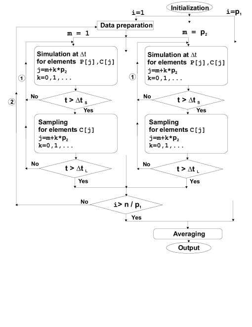
Figure 8: Algorithm of two-level parallelization. $\Delta t$ — time step, $\Delta t_{s}$ — interval between samples, $\Delta t_{L}$ — time of a single run, $t$ — current time, $i$ — run number (first level), $p_{1}$ — number of first level processors, $m$ — second level processor ID-number, $p_{2}$ — number of second level processors, $j$ — index of array element.

statistically independent runs $n$ is significantly less than the number of processors $p$ ($n\ll p$). In this case the efficient usage of computer resources of $p$-processor system can be provided by the implementation of an algorithm of two-level parallelization (TLP algorithm). The general flowchart of TLP algorithm is shown in the fig. 8. The first level of parallelization corresponds to the PSIR algorithm, the data parallelization is employed for the second level inside each independent run. The TLP algorithm is a parallel algorithm with static load balancing.

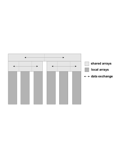
Figure 9: Scheme of memory usage for TLP algorithm ($p_{1}=2$, $p_{2}=3$)

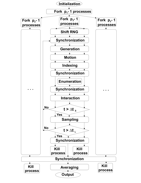
Figure 10: Flowchart of TLP algorithm

The scheme of memory usage for TLP algorithm is depicted in the fig. 9. This algorithm requires the memory size to be proportional to the number of the first level processors which compute single runs (just the same as for the PSIR algorithm). It also requires the arrays for each run to be stored in the shared memory as for the data parallelization algorithm in order to reduce the data exchange time between processors.

The speedup and the efficiency of the TLP algorithm are governed by the following equations:

$$S_{p} = S_{p_{1}}\cdot S_{p_{2}}=\frac{p_{1}}{p_{1}-\alpha_{1}(p_{1}-1)}\,\frac{p_{2}}{p_{2}-\alpha_{2}(p_{2}-1)},$$ (7)

$$E_{p} = E_{p_{1}}\cdot E_{p_{2}}=\frac{S_{p}}{p_{1}\cdot p_{2}},$$ (8)

where indices ‘1’ and ‘2’ correspond to parameters on the first level and on the second one.

The figure 10 shows the detailed flowchart of TLP algorithm for unsteady flow simulation. There are five synchronization points in the algorithm. The four of them correspond to the DP algorithm. The last synchronization has to be done after termination of all runs. The synchronization is employed with the aid of the semaphore technique. In this version the iterations of the outer loop (2) are fully distributed between the first level processors. This algorithm requires $n$ to be multiply by $p$ for uniform distribution of computer resources between single runs. In order to make the runs statistically independent we have to shift the random number generator in each run.

The HP/Convex Exemplar SPP-1600 system with 8 processors, 2Gb of memory and peak performance 1600 Mflops was used for algorithm test.

To simulate the conditions of a single user in the system we measured the execution time of the parent process which makes the start-up initialization before forking child processes and data processing after passing parallel code (this process has the maximum execution time).

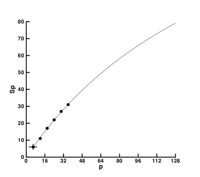
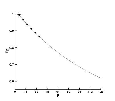
Figure 11: Speedup $S_{p}$ (top) and efficiency $E_{p}$ (bottom) of TLP algorithm (circles — experiment, curve — formulae(7,8), cross — speedup of PSIR algorithm)

The amount of parallel and sequential code was obtained from the program profiling data using standard cxpa utility.

The simulation of unsteady 3-D water vapor flow in the inner atmosphere of a comet was carried out in order to study the speedup and the efficiency which yields this algorithm. The number of the first level processors $p_{1}$ was fixed and equal to 6. The number of the second level processors $p_{2}$ was varied from 1 to 6. The value of parallel fraction $\alpha_{1}$ and $\alpha_{2}$ were 0.998 and 0.97 respectively. The figure 11 depicts the experimental results (circles) and theoretical curves for speedup and efficiency as functions of the total number of processors $p=p_{1}\cdot p_{2}$. The same figure shows the value (marked by cross-sign) of speedup and efficiency of the PSIR algorithm (TLP algorithm turns into PSIR algorithm at $p_{2}=1$).

Thus, the TLP algorithm gives the possibility to significantly reduce the computational time required for the DSMC of unsteady flows using multiprocessor computers with shared memory. The range of the efficient usage of this algorithm is the condition $n\ll p$. Moreover, the number of processors $p$ has to be multiply by $n$ in order to provide good load balancing.

3 Algorithm of Two-Level Parallelization
with Dynamic Load Balancing

The TLP algorithm with static load balancing described in section 2 has several drawbacks. It does not provide good load balancing (hence, one may get low efficiency) in the following cases:

1. the ratio $p/p_{1}$ is not integer (part of processors are not used);

2. each run has non-parallelized code with total sequential fraction equal to $\beta_{\ast}$, which depends on the starting sequential fraction $\beta=1-\alpha$ and the number of processors $p_{2}$:

$$\beta_{\ast}=\frac{\beta}{\beta+\frac{1-\beta}{p_{2}}}.$$ (9)

At small values of $\alpha$ or large values of $p_{2}$ some processors may be idle in each run. This leads to non-efficient usage of computer resources for high values of $p_{1}$.

The increase in efficiency can be obtained by usage of dynamic load balancing with the aid of dynamic processor reallocation (DPR). The idea of the algorithm is as follows. Let us conditionally divide all available processors into two parts: leading processors $p_{1}$ and supporting processors which form the so called “heap” (the number of heap-processors is $p-p_{1}$). Each leading processor is responsible for its own run. This algorithm is similar to that of TLP but here there is no hard link of heap-processors with the specific run. Each leading processor reserves the required number of heap-processors before starting parallel computations (according to a special allocation algorithm). After exiting from parallel procedure the leading processor releases allocated heap-processors. This algorithm makes it possible to use idle processors more efficiently, in fact this leads to execution of parallel code with the aid of more processors than in the case of TLP algorithm with static load balancing. The flowchart of TLPDPR algorithm is presented in the fig. 12.

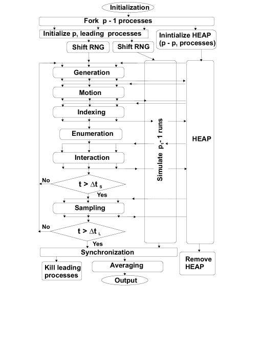
Figure 12: Flowchart of TLPDPR algorithm

The speedup which yields this algorithm is determined by the following basic parameters: the total available number of processors in the system $p$, the required number of independent runs $p_{1}=n$ ($p_{1}\ll p$), the sequential fraction of computational work in each run $\beta$ and the algorithm of heap-processors allocation. In this paper we use the following allocation algorithm:

$$p_{2}^{\prime}=(1+\mathrm{PRI})p_{2},\quad\mathrm{PRI}=0\ldots\mathrm{PRI}^{\ast},$$ (10)

where $p_{2}^{\prime}$ — the actual number of the second level processors, $\mathrm{PRI}$ — the parameter which is estimated by experimental results of similar problems, $\mathrm{PRI}^{\ast}$ — the estimated upper limit of the efficient range of parameter $\mathrm{PRI}$.

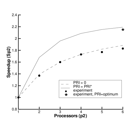
Figure 13: Speedup on the second level as a function of number of second level processors $p_{2}$ for algorithms of TLP ($\mathrm{PRI}=0$, dashed line) and TLPDPR ($\mathrm{PRI}=\mathrm{PRI}^{\ast}$, solid line), circles — experiment ($p_{1}=6$, $p=36$, $\mathrm{PRI}=0$), asterisk — optimal value of parameter $\mathrm{PRI}$

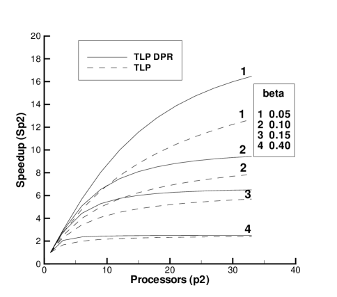
Figure 14: Speedups of TLP (dashed line) and TLPDPR (solid line) algorithms as functions of number of the second level processors $p_{2}$ for various parallel fractions $\beta$ on the second level

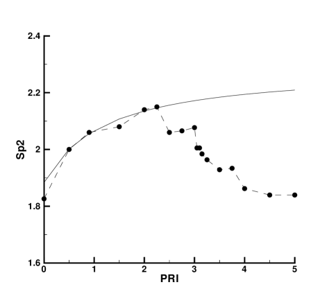
Figure 15: Speedup on the second level $S_{p_{2}}$ as a function of $\mathrm{PRI}$ ($p_{1}=6$, $p=36$,
$\mathrm{PRI}=0\ldots\mathrm{PRI}^{\ast}$). Solid line — theory, dashed line — experiment approximation

In case of $p$ being multiply by $p_{1}$ and the value of $\mathrm{PRI}$ is equal to 0, this algorithm turns into TLP algorithm. The speedup on the second level $S_{p_{2}}$ is governed by the following equation:

$$S_{p_{2}}=\frac{1}{\beta+\frac{1-\beta}{p_{2}(1+\mathrm{PRI})}}.$$ (11)

The case when parameter $\mathrm{PRI}$ exceeds a threshold leads to the decrease of speedup $S_{p_{2}}$. This decrease is not governed by (11) owing to overstating demands made by allocation algorithm on system resources. As a result, this leads to worse load balancing. The upper limit of the efficient range of parameter $\mathrm{PRI}$ can be estimated by the following condition:

$$1+\frac{p-p_{1}}{(1-\beta_{\ast})p_{1}}=(1+\mathrm{PRI}^{\ast})p_{2}.$$ (12)

It means that we have to find such a value of parameter $\mathrm{PRI}$ for which there is a uniform distribution of all idle processors at a given moment among runs which perform parallel computations. The condition for $\mathrm{PRI}^{\ast}$ as a function of $\beta$ and $p_{2}$ can be derived from (9) and (12):

$$\mathrm{PRI}^{\ast}=\frac{\beta}{1-\beta}(p_{2}-1).$$ (13)

The expressions discussed precedingly are undoubtedly correct for $p_{1}\gg 1$. The value of $S_{p_{2}}$ at $\mathrm{PRI}=\mathrm{PRI}^{\ast}$ gives the upper limit of speedup for a given problem.

To study the characteristics of TLPDPR algorithm we solve the problem on unsteady flow past a body. The value of sequential fraction $\beta=0.437$, $p_{1}=6$. The speedup as a function of $p_{2}$ ($p_{2}=1\ldots 6$) for $\mathrm{PRI}=0$ and $\mathrm{PRI}=\mathrm{PRI}^{\ast}$ is depicted in the fig. 13. The same figure shows the results of calculation for $\mathrm{PRI}=0$, the dot (marked by asterisk) corresponds to the optimal value of parameter $\mathrm{PRI}$ for $p_{2}=6$ ($p=36$). The maximum speedup $S_{p_{2}}$ with a given degree of parallelism ($p_{1}\rightarrow\infty$), which can be estimated by the formula (11), comes to 2.3. The TLP algorithm gives the speedup ($\beta=0.437$, $p_{1}=6$, $p=36$) which is 80% of the maximum value. At optimum value of parameter $\mathrm{PRI}$ the TLPDPR algorithm gives 93% for the same case. This is equivalent to the usage of TLP algorithm on a 120-processor computer ($p=120$, $p_{1}=6$, $p_{2}=20$). The figure 14 shows speedups of TLP and TLPDPR algorithms as functions of $p_{2}$ for various $\beta$.

The essential question one can raise about TLPDPR algorithm usage is how to determine the optimal value of parameter $\mathrm{PRI}$ apriori. The value given by (13) determines the upper limit of efficent range of parameter $\mathrm{PRI}=1\ldots\mathrm{PRI}^{\ast}$. The study of influence of parameter $\mathrm{PRI}$ on the speedup is presented in the fig. 15 for $p_{1}=6$, $p_{2}=6$ ($p=36$). The formula (11) gives good approximation of experimental results for the intial range of parameter $\mathrm{PRI}$. Further, we see the predicted above decrease of speedup owing to inconsistency of available and required system resources. The latter can be explained in the following manner. In (11) it is supposed that released heap processors are allocated instantly in the other runs. Actually, these processes are non-coinciding, therefore the condition (11) requires a probability coefficient which is a function of parameters of a problem and a computer. This coefficient has to determine the probability to meet requirements for system resources while allocating heap processors.

The great flexibility of this algorithm allows its efficient usage for calculation of both steady and unsteady problems. In case of steady-state modeling it is possible to perform an additional ensemble averaging for smaller number of modeling particles. This can lead to shorter computation time comparing to DP algorithm. The implemented TLPDPR algorithm has the following advantages comparing to the TLP algorithm with static load balancing:

• TLPDPR algorithm makes it possible to minimize the latency time of processors. It provides better load balancing;

• Better load balancing make it possible to get higher speedups under the same conditions.

References

- [1] G.A.Bird. Molecular Gasdynamics and Direct Simulation of Gas Flows. Clarendon Press. Oxford. 1994
- [2] Korolev, M.Ya. Marov, Yu. Skorov, M. Aspnas. An Implementation of Monte-Carlo weighting method on multiprocessor systems. Reports on Computer Science&Mathematics, Abo Akademy, Ser. A, No. 125, 1991.
- [3] Ota Masahiro, Tanaka Tetsuya. On the parallel processing of Direct Simulation Monte Carlo method. National Aerospace Lab., Proceedings of the 8th NAL Symposium on Aircraft Computational Aerodynamics p. 39-44, Nov 01, 1990.
- [4] N.Y.Bykov, G.A.Lukianov. Parallel Direct Simulation Monte Carlo of Non-stationary Rarefied Gas Flows at the Supercomputers with Parallel Architecture. St.Petersburg. Institute for High-Performance Computing and Databases. Preprint N5-97. 1997.
- [5] Furlani T.R., Lordi J.A. A Comparison of Parallel Algorithms for the Direct Simulation Monte Carlo Method II: Application to Exhaust Plumes Flowfields, AIAA Paper 89-1167, June 1989.
- [6] Wilmoth R.G. Adaptive Domain Decomposition for Monte Carlo Simulations on Parallel Processor. In. 17th Rarefied Gas Dynamics Symposium. AIAA, July 1990.
- [7] Boyd I.D., Dietrich S. A Scalar Optimized Parallel Implementation of the DSMC Method, AIAA Paper 94-0355, January 1994.
- [8] Boyd I.D., Dietrich S. Scalar and Parallel Optimized Implementation of the Direct Simulation Monte Carlo Method, J. Comp. Phys., 1996, vol. 126, p. 328-342.
- [9] Ivanov, M., Markelov, G., Tylor, S., Watts J. Parallel DSMC Strategies for 3D Computations, Parallel CFD’96, P. Schiano et al. eds., North Holland, Amsterdam, 1997, pp. 485-492.
- [10] Robinson C.D., Harvey J.K. The Development of an Efficient Direct Simulation Monte Carlo Computation Scheme for Gas Flows in a Parallel Environment. In Proceedings of the Fourth International Parallel Computing Workshop, Imperial College/Fujitsu Parallel Computing Research Centre, Imperial College, London, 1995. Copies available from author.
- [11] Robinson C.D., Harvey J.K. Adaptive Domain Decomposition for Unstructured Meshes Applied to the Direct Simulation Monte Carlo Method. In J. Periaux, P. Schiano, A. Ecer and N. Satofuka, editors, Proceedings Parallel CFD 96. Elsever, 1996.
- [12] Oh C.K., Sinkovis R.S., Cybyk B.Z., Oran E.S.,Boris J.P. Parallelization of Direct Simulation Monte Carlo Method Combined with Monotonic Lagrangian Grid, AIAA J. vol. 34, N7, July 1996, p. 1363.
- [13] I.A.Grishin, V.V.Zakharov, G.A.Lukianov. Data Parallelization of Direct Simulation Monte Carlo in Gasdynamics. St.Petersburg. Institute for High-Performance Computing and Databases. Preprint N3-98. 1998.
- [14] A.V.Bogdanov, N.Y.Bykov, G.A.Lukianov. Distributed and Parallel Direct Simulation Monte Carlo of Rarefied Gas Flows. Lecture Notes in Computer Science, Vol. 1401. Springer-Verlag, Berlin Heidelberg New York (1998)
- [15] J.M.Ortega. Introduction to Parallel and Vector Solution of Linear Systems. Plenum Press. New York. 1988