Forgetting Exceptions is Harmful in Language Learning

Abstract

We show that in language learning, contrary to received wisdom, keeping exceptional training instances in memory can be beneficial for generalization accuracy. We investigate this phenomenon empirically on a selection of benchmark natural language processing tasks: grapheme-to-phoneme conversion, part-of-speech tagging, prepositional-phrase attachment, and base noun phrase chunking. In a first series of experiments we combine memory-based learning with training set editing techniques, in which instances are edited based on their typicality and class prediction strength. Results show that editing exceptional instances (with low typicality or low class prediction strength) tends to harm generalization accuracy. In a second series of experiments we compare memory-based learning and decision-tree learning methods on the same selection of tasks, and find that decision-tree learning often performs worse than memory-based learning. Moreover, the decrease in performance can be linked to the degree of abstraction from exceptions (i.e., pruning or eagerness). We provide explanations for both results in terms of the properties of the natural language processing tasks and the learning algorithms.

1 Introduction

Memory-based reasoning [Stanfill and Waltz,1986] is founded on the hypothesis that performance in real-world tasks (in our case language processing) is based on reasoning on the basis of similarity of new situations to stored representations of earlier experiences, rather than on the application of mental rules abstracted from earlier experiences as in rule-based processing. The type of learning associated with such an approach is called lazy learning [Aha,1997]. The approach has surfaced in different contexts using a variety of alternative names such as example-based, exemplar-based, analogical, case-based, instance-based, locally weighted, and memory-based [Stanfill and Waltz,1986, Cost and Salzberg,1993, Kolodner,1993, Aha, Kibler, and Albert,1991, Atkeson, Moore, and Schaal,1997]. Historically, lazy learning algorithms are descendants of the $k$-nearest neighbor (henceforth $k$-nn) classifier [Cover and Hart,1967, Devijver and Kittler,1982, Aha, Kibler, and Albert,1991].

Memory-based learning is ‘lazy’ as it involves adding training examples (feature-value vectors with associated categories) to memory without abstraction or restructuring. During classification, a previously unseen test example is presented to the system. Its similarity to all examples in memory is computed using a similarity metric, and the category of the most similar example(s) is used as a basis for extrapolating the category of the test example. A key feature of memory-based learning is that, normally, all examples are stored in memory and no attempt is made to simplify the model by eliminating noise, low frequency events, or exceptions. Although it is clear that noise in the training data can harm accurate generalization, this work focuses on the problem that, for language learning tasks, it is very difficult to discriminate between noise on the one hand, and valid exceptions and sub-regularities that are important for reaching good accuracy on the other hand.

The goal of this paper is to provide empirical evidence that for a range of language learning tasks, memory-based learning methods tend to achieve better generalization accuracies than (i) memory-based methods combined with training set editing techniques in which exceptions are explicitly forgotten, i.e. removed from memory, and (ii) decision-tree learning in which some of the information from the training data is either forgotten (by pruning) or made inaccessible (by the eager construction of a model). We explain these results in terms of the data characteristics of the tasks, and the properties of memory-based learning. In our experiments we compare ib1-ig [Daelemans and Van den Bosch,1992, Daelemans, Van den Bosch, and Weijters,1997], a memory-based learning algorithm, with (i) edited versions of ib1-ig, and (ii) decision-tree learning in c5.0 [Quinlan,1993] and in igtree [Daelemans, Van den Bosch, and Weijters,1997]. These learning methods are described in Section 2. The compared algorithms are applied to a selection of four natural language processing (nlp) tasks (described in Section 3). These tasks present a varied sample of the complete domain of nlp as they relate to phonology and morphology (grapheme-to-phoneme conversion); morphology and syntax (part of speech tagging, base noun phrase chunking); and syntax and lexical semantics (prepositional-phrase attachment).

First, we show in Section 4 that two criteria for editing instances in memory-based learning, viz. low typicality and low class prediction strength, are generally responsible for a decrease in generalization accuracy.

Second, memory-based learning is demonstrated in Section 5 to be mostly at an advantage, and sometimes at a par with decision-tree learning as far as generalization accuracy is concerned. The advantage is puzzling at first sight, as ib1-ig, c5.0 and igtree are based on similar principles: (i) classification of test instances on the basis of their similarity to training instances (in the form of the instances themselves in ib1-ig or in the form of hyper-rectangles containing subsets of partly-similar training instances in c5.0 and igtree), and (ii) use of information entropy as a heuristic to constrain the space of possible generalizations (as a feature weighting method in ib1-ig, and as a split criterion in c5.0 and igtree).

Our hypothesis is that both effects are due to the fact that ib1-ig keeps all training instances as possible sources for classification, whereas both the edited versions of ib1-ig and the decision-tree learning algorithms c5.0 and igtree make abstractions from irregular and low-frequency events. In language learning tasks, where sub-regularities and (small families of) exceptions typically abound, the latter is detrimental to generalization performance. Our results suggest that forgetting exceptional training instances is harmful to generalization accuracy for a wide range of language-learning tasks. This finding contrasts with a consensus in supervised machine learning that forgetting exceptions by pruning boosts generalization accuracy [Quinlan,1993], and with studies emphasizing the role of forgetting in learning [Markovitch and Scott,1988, Salganicoff,1993].

Section 6 places our results in a broader machine learning and language learning context, and attempts to describe the properties of language data and memory-based learning that are responsible for the ‘forgetting exceptions is harmful’ effect. For our data sets, the abstraction and pruning techniques studied do not succeed in reliably distinguishing noise from productive exceptions, an effect we attribute to a special property of language learning tasks: the presence of many exceptions that tend to occur in groups or pockets in instance space, together with noise introduced by corpus coding methods. In such a situation, the best strategy is to keep all training data to generalize from.

2 Learning methods

In this Section, we describe the three algorithms we used in our experiments. ib1-ig is used for studying the effect of editing exceptional training instances, and in a comparison to the decision tree methods c5.0 and igtree.

2.1 IB1-IG

ib1-ig [Daelemans and Van den Bosch,1992, Daelemans, Van den Bosch, and Weijters,1997] is a memory-based (lazy) learning algorithm that builds a data base of instances (the instance base) during learning. An instance consists of a fixed-length vector of $n$ feature-value pairs, and a field containing the classification of that particular feature-value vector. After the instance base is built, new (test) instances are classified by matching them to all instances in the instance base, and by calculating with each match the distance between the new instance $X$ and the stored instance $Y$.

The most basic metric for instances with symbolic features is the overlap metric given in Equations 1 and 2; where $\Delta(X,Y)$ is the distance between instances $X$ and $Y$, represented by $n$ features, $w_{i}$ is a weight for feature $i$, and $\delta$ is the distance per feature. The $k$-nn algorithm with this metric, and equal weighting for all features is, for example, implemented in ib1 [Aha, Kibler, and Albert,1991]. Usually $k$ is set to 1.

$$\Delta(X,Y)=\sum_{i=1}^{n}\ w_{i}\ \delta(x_{i},y_{i})$$ (1)

where:

$$\delta(x_{i},y_{i})=0\ if\ x_{i}=y_{i},\ else\ 1$$ (2)

We have made two additions to the original algorithm in our version of ib1. First, in the case of nearest neighbor sets larger than one instance ($k>1$ or ties), our version of ib1 selects the classification with the highest frequency in the class distribution of the nearest neighbor set. Second, if a tie cannot be resolved in this way because of equal frequency of classes among the nearest neighbors, the classification is selected with the highest overall occurrence in the training set.

The distance metric in Equation 2 simply counts the number of (mis)matching feature values in both instances. In the absence of information about feature relevance, this is a reasonable choice. Otherwise, we can add linguistic bias to weight or select different features [Cardie,1996] or look at the behavior of features in the set of examples used for training. We can compute statistics about the relevance of features by looking at which features are good predictors of the class labels. Information theory gives us a useful tool for measuring feature relevance in this way [Quinlan,1986, Quinlan,1993].

Information gain (IG) weighting looks at each feature in isolation, and measures how much information it contributes to our knowledge of the correct class label. The information gain of feature $f$ is measured by computing the difference in uncertainty (i.e. entropy) between the situations without and with knowledge of the value of that feature (Equation 3).

$$w_{f}=\frac{H(C)-\sum_{v\in V_{f}}P(v)H(C|v)}{si(f)}$$ (3)

$$si(f)=-\sum_{v\in V_{f}}P(v)\log_{2}P(v)$$ (4)

where $C$ is the set of class labels, $V_{f}$ is the set of values for feature $f$, and $H(C)=-\sum_{c\in C}P(c)\log_{2}P(c)$ is the entropy of the class label probability distribution. The probabilities are estimated from relative frequencies in the training set. The normalizing factor $si(f)$ (split info) is included to avoid a bias in favor of features with more values. It represents the amount of information needed to represent all values of the feature (Equation 4). The resulting IG values can then be used as weights in equation 1.

The possibility of automatically determining the relevance of features implies that many different and possibly irrelevant features can be added to the feature set. This is a very convenient methodology if theory does not constrain the choice enough beforehand, or if we wish to measure the importance of various information sources experimentally. A limitation is its insensitivity to feature redundancy; although a feature may be redundant, it may be assigned a high information gain weight. Nevertheless, the advantages far outweigh the limitations for our data sets, and ib1-ig consistently outperforms ib1.

2.2 C5.0

c5.0, a commercial version of c4.5 [Quinlan,1993], performs top-down induction of decision trees (tdidt). On the basis of an instance base of examples, c5.0 constructs a decision tree which compresses the classification information in the instance base by exploiting differences in relative importance of different features. Instances are stored in the tree as paths of connected nodes ending in leaves which contain classification information. Nodes are connected via arcs denoting feature values. Feature information gain (Equation 3) is used dynamically in c5.0 to determine the order in which features are employed as tests at all levels of the tree [Quinlan,1993].

c5.0 can be tuned by several parameters. In our experiments, we chose to vary the pruning confidence level (the $c$ parameter), and the minimal number of instances represented at any branch of any feature-value test (the $m$ parameter). The two parameters directly affect the degree of ‘forgetting’ of individual instances by c5.0:

• The $c$ parameter denotes the pruning confidence level, which ranges between 0% and 100%. This parameter is used in a heuristic function that estimates the predicted number of misclassifications of unseen instances at leaf nodes, by computing the binomial probability (i.e, the confidence limits for the binomial distribution) of misclassifications within the set of instances represented at that node [Quinlan,1993]. When the presence of a leaf node leads to a higher predicted number of errors than when it would be absent, it is pruned from the tree. By default, $c=25\%$; set at 100%, no pruning occurs. The more pruning is performed, the less information about the individual examples is remembered in the abstracted decision tree.

• The $m$ parameter governs the minimum number of instances represented by a node. By setting $m>1$, c5.0 can avoid the creation of long paths disambiguating single-instance minorities that possibly represent noise [Quinlan,1993]. By default, $m=2$. With $m=1$, c5.0 builds a path for every single instance not yet disambiguated. Higher values of $m$ lead to an increasing amount of abstraction and therefore to less recoverable information about individual instances.

Moreover, we chose to set the subsetting of values ($s$) parameter at the non-default value ‘on’. The $s$ parameter is a flag determining whether different values of the same feature are grouped on the same arc in the decision tree when they lead to identical or highly similar subtrees. We used value grouping as a default for reasons of computational complexity for the pos, pp, and np data sets, and because that setting yields higher generalization accuracy for the gs data set.

2.3 IGTREE

The igtree algorithm was originally developed as a method to compress and index case bases in memory-based learning [Daelemans, Van den Bosch, and Weijters,1997]. It performs tdidt in a way similar to that of c5.0, but with two important differences. First, it builds oblivious decision trees, i.e., feature ordering is computed only at the root node and is kept constant during tdidt, instead of being recomputed at every new node. Second, igtree does not prune exceptional instances; it is only allowed to disregard information redundant for the classification of the instances presented during training.

Instances are stored as paths of connected nodes and leaves in a decision tree. Nodes are connected via arcs denoting feature values. The global information gain of the features is used to determine the order in which instance feature values are added as arcs to the tree. The reasoning behind this compression is that when the computation of information gain points to one feature clearly being the most important in classification, search can be restricted to matching a test instance to those memory instances that have the same feature value as the test instance at that feature. Instead of indexing all memory instances only once on this feature, the instance memory can then be optimized further by examining the second most important feature, followed by the third most important feature, etc. A considerable compression is obtained as similar instances share partial paths.

The tree structure is compressed even more by restricting the paths to those input feature values that disambiguate the classification from all other instances in the training material. The idea is that it is not necessary to fully store an instance as a path when only a few feature values of the instance make the instance classification unique. This implies that feature values that do not contribute to the disambiguation of the instance (i.e., the values of the features with lower information gain values than the lowest information gain value of the disambiguating features) are not stored in the tree.

Apart from compressing all training instances in the tree structure, the igtree algorithm also stores with each non-terminal node information concerning the most probable or default classification given the path thus far, according to the bookkeeping information maintained by the tree construction algorithm. This extra information is essential when processing unknown test instances. Processing an unknown input involves traversing the tree (i.e., matching all feature-values of the test instance with arcs in the order of the overall feature information gain), and either retrieving a classification when a leaf is reached (i.e., an exact match was found), or using the default classification on the last matching non-terminal node if an exact match fails.

In sum, in the trade-off between computation during learning and computation during classification, the igtree approach chooses to invest more time in organizing the instance base than ib1-ig, but less than c5.0, because the order of the features needs to be computed only once for the whole data set.

3 Benchmark language learning tasks

We investigate four language learning tasks that jointly represent a wide range of different types of tasks in the nlp domain: (1) grapheme-phoneme conversion (henceforth referred to as gs), (2) part-of-speech tagging (pos), (3) prepositional-phrase attachment (pp), and (4) base noun phrase chunking (np). In this section, we introduce each of the four tasks, and describe for each task the data collected and employed in our study. First, properties of the four data sets are listed in Table 1, and examples of instances for each of the tasks are displayed in Table 2.

	#	# Values of feature											#	# Data set
Task	Features	1	2	3	4	5	6	7	8	9	10	11	Classes	instances
gs	7	42	42	42	41	42	42	42					159	675,745
pos	5	170	170	498	492	480							169	1,046,152
pp	4	3,474	4,612	68	5,780								2	23,898
np	11	20,231	20,282	20,245	20,263	86	87	86	89	3	3	3	3	251,124

Table 1: Properties of the four investigated data sets of the gs, pos, pp, and np learning tasks: numbers of features, values per feature, classes, and instances.

	Features
Task	1	2	3	4	5	6	7	8	9	10	11	label
gs	_	h	e	a	r	t	s					0A:
	b	o	o	k	i	n	g					0k
	t	i	e	s	_	_	_					0z
	_	_	a	f	a	r	_					1f
pos	_	sqso	VB	vbg	nn							vb
	nns	bez	TO/IN	be	vbn/vbd							to
	np	hvz	VB/VBN/VBD	rp/in	at							vbn
	_	_	PP3	md	rn							pp3
pp	is	chairman	of	NV								noun
	pour	cash	into	funds								verb
	asked	them	for	views								verb
	caused	swings	in	prices								noun
np	definitive	agreement	between	the	jj	nn	in	dt	I	I	I	O
	when	they	need	money	wrb	pp	vbp	nn	I	I	O	O
	pose	a	new	challenge	vb	dt	jj	nn	O	I	I	I
	performance	that	would	compare	nn	wdt	md	vb	O	B	I	O

Table 2: Example of instances of the gs, pos, pp, and np learning tasks. All instances represent fixed-sized feature-value vectors and an associated class label. Feature values printed in bold are focus features (description in text).

3.1 GS: grapheme-phoneme conversion with stress assignment

Converting written words to stressed phonemic transcription, i.e., word pronunciation, is a well-known benchmark task in machine learning [Sejnowski and Rosenberg,1987, Stanfill and Waltz,1986, Stanfill,1987, Lehnert,1987, Wolpert,1989, Shavlik, Mooney, and Towell,1991, Dietterich, Hild, and Bakiri,1995]. We define the task as the conversion of fixed-sized instances representing parts of words to a class representing the phoneme and the stress marker of the instance’s middle letter. We henceforth refer to the task as gs, an acronym of grapheme-phoneme conversion and stress assignment. To generate the instances, windowing is used [Sejnowski and Rosenberg,1987]. Table 2 (top) displays four example instances and their classifications. Classifications, i.e., phonemes with stress markers, are denoted by composite labels. For example, the first instance in Table 2, _hearts, maps to class label 0A:, denoting an elongated short ‘a’-sound which is not the first phoneme of a syllable receiving primary stress. In this study, we chose a fixed window width of seven letters, which offers sufficient context information for adequate performance (in terms of the upper bound on error demanded by applications in speech technology).

From celex [Baayen, Piepenbrock, and van Rijn,1993] we extracted, on the basis of the standard word base of 77,565 words with their corresponding transcription, a data base containing 675,745 instances. The number of classes (i.e., all possible combinations of phonemes and stress markers) occurring in this data base is 159.

3.2 POS: Part-of-speech tagging of word forms in context

Many words in a text are ambiguous with respect to their morphosyntactic category (part-of-speech). Each word has a set of lexical possibilities, and the local context of the word can be used to select the most likely category from this set [Church,1988]. For example in the sentence “they can can a can”, the word can is tagged as modal verb, main verb and noun respectively. We assume a tagger architecture that processes a sentence from the left to the right by classifying instances representing words in their contexts (as described in [Daelemans et al.,1996]). The word’s already tagged left context is represented by the disambiguated categories of the two words to the left, the word itself and its ambiguous right context are represented by categories which denote ambiguity classes (e.g. verb-or-noun).

The data set for the part-of-speech tagging task, henceforth referred to as the pos task, was extracted from the LOB corpus. The full data set contains 1,046,152 instances. The “lexicon” of ambiguity classes was constructed from the first 90% of the corpus only, and hence the data contains unknown words. To avoid a complicated architecture, we treat unknown words the same as the known words, i.e., their ambiguous category is simply “unknown”, and they can only be classified on the basis of their context.

3.3 PP: Disambiguating verb/noun attachment of prepositional phrases

As an example of a semantic-syntactic disambiguation task we consider a simplified version of the task of Prepositional Phrase (henceforth pp) attachment: the attachment of a PP in the sequence VP NP PP (VP $=$ verb phrase, NP $=$ noun phrase, PP $=$ prepositional phrase). The data consists of four-tuples of words, extracted from the Wall Street Journal Treebank [Marcus, Santorini, and Marcinkiewicz,1993] by a group at ibm [Ratnaparkhi, Reynar, and Roukos,1994]. They took all sentences that contained the pattern VP NP PP and extracted the head words from the constituents, yielding a V N1 P N2 pattern (V $=$ verb, N $=$ noun, P $=$ preposition). For each pattern they recorded whether the PP was attached to the verb or to the noun in the treebank parse. For example, the sentence “he eats pizza with a fork” would yield the pattern:

eats, pizza, with, fork, verb.

because here the PP is an instrumental modifier of the verb. A contrasting sentence would be “he eats pizza with anchovies”, where the PP modifies the noun phrase pizza.

eats, pizza, with, anchovies, noun.

From the original data set, used in statistical disambiguation methods by [Ratnaparkhi, Reynar, and Roukos,1994] and [Collins and Brooks,1995], we took the train and test set together to form a new data set of 23,898 instances.

Due to the large number of possible word combinations and the comparatively small training set size, this data set can be considered very sparse. Of the 2390 test instances in the first fold of the 10 cross-validation (CV) partitioning, only 121 (5.1%) occurred in the training set; 619 (25.9 %) instances had 1 mismatching word with any instance in the training set; 1492 (62.4%) instances had 2 mismatches; and 158 (6.6 %) instances had 3 mismatches. Moreover, the test set contains many words that are not present in any of the instances in the training set.

The pp data set is also known to be noisy. [Ratnaparkhi, Reynar, and Roukos,1994] performed a study with three human subjects, all experienced treebank annotators, who were given a small random sample of the test sentences (either as four-tuples or as full sentences), and who had to give the same binary decision. The humans, when given the four-tuple, gave the same answer as the Treebank parse only 88.2% of the time, and when given the whole sentence, only 93.2% of the time.

3.4 NP: Base noun phrase chunking

Phrase chunking is defined as the detection of boundaries between phrases (e.g., noun phrases or verb phrases) in sentences. Chunking can be seen as a ‘light’ form of parsing. In NP chunking, sentences are segmented into non-recursive NP’s, so called baseNP’s [Abney,1991]. NP chunking can, for example, be used to reduce the complexity of sub-sequential parsing, or to identify named entities for information retrieval. To perform this task, we used the baseNP tag set as presented in [Ramshaw and Marcus,1995]: $I$ for inside a baseNP, $O$ for outside a baseNP, and $B$ for the first word in a baseNP following another baseNP. As an example, the IOB tagged sentence: “The/I postman/I gave/O the/I man/I a/B letter/I ./O” will result in the following baseNP bracketed sentence: “[The postman] gave [the man] [a letter].” The data we used are based on the same material as [Ramshaw and Marcus,1995] which is extracted from the Wall Street Journal text in the parsed Penn Treebank [Marcus, Santorini, and Marcinkiewicz,1993]. Our NP chunker consists of two stages, and in this paper we have used instances from the second stage. An instance (constructed for each focus word) consists of features referring to words, POS tags, and IOB tags (predicted by the first stage) of the focus and the two immediately adjacent words. The data set contains a total of 251,124 instances.

3.5 Experimental method

We used 10-fold CV [Weiss and Kulikowski,1991] in all experiments comparing classifiers (Section 5). In this approach, the initial data set (at the level of instances) is partitioned into ten subsets. Each subset is taken in turn as a test set, and the remaining nine combined to form the training set. Means are reported, as well as standard deviation from the mean. In the editing experiments (Section 4), the first train-test partition of the 10-fold CV was used for comparing the effect on the test set accuracy of applying different editing schemes on the training set.

Having introduced the machine learning methods and data sets that we focus on in this paper, and the experimental method we used, the next Section describes empirical results from a first set of experiments aimed at getting more insight into the effect of editing exceptional instances in memory-based learning.

4 Editing exceptions in memory-based learning is harmful

The editing of instances from memory in memory-based learning or the $k$-nn classifier [Hart,1968, Wilson,1972, Devijver and Kittler,1980] serves two objectives: to minimize the number of instances in memory for reasons of speed or storage, and to minimize generalization error by removing noisy instances, prone to being responsible for generalization errors. Two basic types of editing, corresponding to these goals, can be found in the literature:

• Editing superfluous regular instances: delete instances for which the deletion does not harm the classification accuracy of their own class in the training set [Hart,1968].

• Editing unproductive exceptions: deleting instances that are incorrectly classified by their neighborhood in the training set [Wilson,1972], or roughly vice-versa, deleting instances that are bad class predictors for their neighborhood in the training set [Aha, Kibler, and Albert,1991].

We present experiments in which both types of editing are employed within the ib1-ig algorithm (Subsection 2.1). The two types of editing are performed on the basis of two criteria that estimate the exceptionality of instances: typicality [Zhang,1992] and class prediction strength [Salzberg,1990] (henceforth referred to as cps). Unproductive exceptions are edited by taking the instances with the lowest typicality or cps, and superfluous regular instances are edited by taking the instances with the highest typicality or cps. Both criteria are described in Subsection 4.1. Experiments are performed using the ib1-ig implementation of the TiMBL software package [Daelemans et al.,1998]. We present the results of the editing experiments in Subsection 4.2.

4.1 Two editing criteria

We investigate two methods for estimating the (degree of) exceptionality of instance types: typicality and class prediction strength (cps).

4.1.1 Typicality

In its common meaning, “typicality” denotes roughly the opposite of exceptionality; atypicality can be said to be a synonym of exceptionality. We adopt a definition from [Zhang,1992], who proposes a typicality function. Zhang computes typicalities of instance types by taking the notions of intra-concept similarity and inter-concept similarity [Rosch and Mervis,1975] into account. First, Zhang introduces a distance function which extends Equation 1; it normalizes the distance between two instances $X$ and $Y$ by dividing the summed squared distance by $n$, the number of features. The normalized distance function used by Zhang is given in Equation 5.

$$\Delta(X,Y)=\sqrt{\frac{1}{n}\sum_{i=1}^{n}(\delta(x_{i},y_{i}))^{2}}$$ (5)

The intra-concept similarity of instance $X$ with classification $C$ is its similarity (i.e., $1-$distance) with all instances in the data set with the same classification $C$: this subset is referred to as $X$’s family, $Fam(X)$. Equation 6 gives the intra-concept similarity function $Intra(X)$ ($|Fam(X)|$ being the number of instances in $X$’s family, and $Fam(X)_{i}$ the $i$th instance in that family).

$$Intra(X)=\frac{1}{|Fam(X)|}\sum_{i=1}^{|Fam(X)|}1.0-\Delta(X,Fam(X)_{i})$$ (6)

All remaining instances belong to the subset of unrelated instances, $Unr(X)$. The inter-concept similarity of an instance $X$, $Inter(X)$, is given in Equation 7 (with $|Unr(X)|$ being the number of instances unrelated to $X$, and $Unr(X)_{i}$ the $i$th instance in that subset).

$$Inter(X)=\frac{1}{|Unr(X)|}\sum_{i=1}^{|Unr(X)|}1.0-\Delta(X,Unr(X)_{i})$$ (7)

The typicality of an instance $X$, $Typ(X)$, is $X$’s intra-concept similarity divided by $X$’s inter-concept similarity, as given in Equation 8.

$$Typ(X)=\frac{Intra(X)}{Inter(X)}$$ (8)

An instance type is typical when its intra-concept similarity is larger than its inter-concept similarity, which results in a typicality larger than 1. An instance type is atypical when its intra-concept similarity is smaller than its inter-concept similarity, which results in a typicality between 0 and 1. Around typicality value 1, instances cannot be sensibly called typical or atypical; [Zhang,1992] refers to such instances as boundary instances.

We adopt typicality as an editing criterion here, and use it for editing instances with low typicality as well as instances with high typicality. Low-typical instances can be seen as exceptions, or bad representatives of their own class and could therefore be pruned from memory, as one can argue that they cannot support productive generalizations. This approach has been advocated by [Ting,1994a] as a method to achieve significant improvements in some domains. Editing atypical instances would, in this line of reasoning, not be harmful to generalization, and chances are that generalization would even improve under certain conditions [Aha, Kibler, and Albert,1991]. High-typical instances, on the other hand, may be good predictors for their own class, but there may be enough of them in memory, so that a few may also be edited without harmful effects to generalization.

Table 3 provides examples of low-typical (for each task, the top three) and high-typical (bottom three) instances of all four tasks. The gs examples show that loan words such as czech introduce peculiar spelling-pronunciation relations; particularly foreign spellings turn out to be low-typical. High-typical instances are parts of words of which the focus letter is always pronounced the same way. Low-typical pos instances tend to involve inconsistent or noisy associations between an unambiguous word class of the focus word and a different word class as classification: such inconsistencies can be largely attributed to corpus annotation errors. Focus tags of high-typical pos instances are already unambiguous. The examples of low-typical pp instances represent minority exceptions or noisy instances in which it is questionable whether the chosen classification is right (recall that human annotators agree only on 88% of the instances in the data set, cf. Subsection 3), while the high-typical pp examples have the preposition ‘of’ in focus position, which typically attaches to the noun. Low-typical np instances seem to be partly noisy, and otherwise difficult to interpret. High-typical np instances are clear-cut cases in which a noun occurring between a determiner and a finite verb is correctly classified as being inside an NP.

gs
feature values	class	typicality
u r e a u c r	0@U	0.43
f r e u d i a	0OI	0.44
_ _ c z e c h	0-	0.54
b j e c t i o	0kS	10.57
l k - o v e r	2@U	10.39
e y - j a c k	2_	9.41
pos
feature values	class	typicality
sxm sqsc cc to/in vb	fw	0.05
cd nnu nn bo aa	aq	0.07
pp3os do cc vb pp3as	cs	0.08
cs3 cs4 pp1as nn/jjb/in pp3os	pp1as	3531.53
cs1 cs2 cd nnu1/in nnu2	cd	2887.29
nn2 in2 cd nnu/zz in/cc	cd	2526.98
pp
feature values	class	typicality
accuses Motorola of turnabout	verb	0.01
cleanse Germany of muck	verb	0.01
directs flow through systems	noun	0.02
excluding categories of food	noun	94.52
underscoring lack of stress	noun	94.52
calls frenzy of legislating	noun	94.53
np
feature values	class	typicality
generally a bit safer rb dt nn jjr O O O	O	0.27
“ No matter how “ dt nn wrb O O O	O	0.27
I know that voluntarily pp vbp in rb O O B	I	0.27
that the legislator wins in dt nn vbz O B B	I	6.93
that the bank supports in dt nn vbz O B B	I	6.94
that the company hopes in dt nn vbz O B B	I	6.97

Table 3: Examples of low-typical (top three) and high-typical (bottom three) instances of the gs, pos, pp, and np learning tasks. For each instance its typicality value is given.

4.1.2 Class-prediction strength

A second estimate of exceptionality is to measure how well an instance type predicts the class of all other instance types within the training set. Several functions for computing class-prediction strength have been proposed, e.g., as a criterion for removing instances in memory-based ($k$-nn) learning algorithms, such as ib3 [Aha, Kibler, and Albert,1991] (cf. earlier work on edited $k$-nn [Hart,1968, Wilson,1972, Devijver and Kittler,1980, Voisin and Devijver,1987]); or for weighting instances in the Each algorithm [Salzberg,1990]. We use the class-prediction strength function as proposed by [Salzberg,1990]. This is the ratio of the number of times the instance type is a nearest neighbor of another instance with the same class and the number of times that the instance type is the nearest neighbor of another instance type regardless of the class. An instance type with class-prediction strength 1.0 is a perfect predictor of its own class; a class-prediction strength of 0.0 indicates that the instance type is a bad predictor of classes of other instances, presumably indicating that the instance type is exceptional. Even more than with typicality, one might argue that bad class predictors can be edited from the instance base. Likewise, one could also argue that instances with a maximal cps could be edited to some degree too without harming generalization: strong class predictors may be abundant and some may be safely forgotten since other instance types may be strong enough to support the class predictions of the edited instance type.

In Table 4, examples from the four tasks of instances with low (top three) and high (bottom three) cps are displayed. Many instances with low cps are minority ambiguities. For instance, the gs examples represent instances which are completely ambiguous and of which the classification is the minority. For example, there are more words beginning with algo that have primary stress (class ‘1ae’) than secondary stress (class ‘2ae’), which makes the instance ‘___algo 2ae’ a minority ambiguity.

gs
feature values	class	cps
_ _ _ a l g o	2ae	0.00
c k - b e n c	1b	0.00
e r b y _ _ _	0aI	0.00
_ _ _ w e e k	1w	1.00
a i n d e r s	0d	1.00
e r a c t e d	0k	1.00
pos
feature values	class	cps
scom npt in np np/nn	in	0.00
== == npt np genm/bez	nn	0.00
ati nns vbn/vbd in np	vbd	0.00
sqso wrb xnot vb ati	xnot	1.00
ber cd nns in nn	nns	1.00
at jnp nn vbz in	nn	1.00
pp
feature values	class	cps
allowed access notwithstanding designations	verb	0.00
had yield during week	noun	0.00
make commodity of luxury	verb	0.02
is one of strategy	noun	0.99
is one of restructuring	noun	0.99
is one of program	noun	0.99
np
feature values	class	cps
of KLM Royal Dutch in np np np I I O	I	0.00
in ethics charges against in nns nns in O I O	I	0.00
assets . The axiom nns stop dt nn I O I	I	0.00
I drink to your pp vbp to pp I O I	I	1.00
share price could zoom nn nn md vb I I O	O	1.00
work force as well nn nn rb rb O I I	O	1.00

Table 4: Examples of instances with low class prediction strength (top three) and high class prediction strength (bottom three) of the gs, pos, pp, and np tasks. For each instance its class prediction strength (cps) value is given.

To test the utility of these measures as criteria for justifying forgetting of specific training instances, we performed a series of experiments in which ib1-ig is applied to the four data sets, systematically edited according to each of four tested criteria. We performed the editing experiments on the first fold of the 10-fold CV partitioning of the four data sets. For each editing criterion (i.e., low and high typicality, and low and high cps), we created eight edited instance bases by removing 1%, 2%, 5%, 10%, 20%, 30%, 40%, and 50% of the instance tokens (rounded off so as to remove a whole number of instance types) according to the criterion from a single training set (the training set of the first 10-fold CV partition). ib1-ig was then trained on each of the edited training sets, and tested on the original unedited test set (of the first 10-fold CV partition).

Figure 1: The percentage of instance types that are edited by both the typicality and the class prediction strength criterion. The left part of the figure shows the results for editing exceptional instances, the right part shows the results for editing regular instances.

To measure to what degree the two criteria are indeed different measures of exceptionality, the percentage of overlap between the removed types was measured for each data set. As can be seen in Figure 1, the two measures mostly have fairly little overlap, certainly for editing below 10%. The reason for this is that typicality is based on global properties of the data set, whereas class prediction strength is based only on the local neighborhood of each instance. Only for the PP attachment and POS tagging tasks do the sets of edited exceptional instances overlap up to 70% when editing 10%.

4.2 Editing exceptions: Results

The general trend we observe in the results obtained with the editing experiments is that editing on the basis of typicality and class-prediction strength, whether low or high, is not beneficial, and is ultimately harmful to generalization accuracy. More specifically, we observe a trend that editing instance types with high typicality or high cps is less harmful than editing instance types with low typicality or low class prediction strength – again, with some exceptions. The results are summarized in Figure 2. The results show that in any case for our data sets, editing serves neither of its original goals. If the goal is a decrease of speed and memory requirements, editing criteria should allow editing of 50% or more without a serious decrease in generalization accuracy. Instead, we see disastrous effects on generalization accuracy at much lower editing rates, sometimes even at 1%. When the goal is improving generalization accuracy by removing noise, the focus of the editing experiments in this paper, none of the studied criteria turns out to be useful.

Figure 2: Generalization accuracies (in terms of % of correctly classified test instances) of ib1-ig on the four tasks with increasing percentages of edited instance tokens, according to the four tested editing criteria.

To compute the statistical significance of the effect of editing, the output for each criterion was compared to the correct classification and the output of the unedited classifier. The resulting cross-tabulation of hits and misses was subjected to McNemar’s $\chi^{2}$ test [Dietterich,1998 in press]. Differences with $p<0.05$ are reported as significant.

A detailed look at the results per data set shows the following results. Editing experiments on the gs task (top left of Figure 2) show significant decreases in generalization accuracy with all editing criteria and all amounts (even 1% is harmful); editing on the basis of low and high cps is particularly harmful, and all criteria except low typicality show a dramatic drop in accuracy at high levels of editing.

The editing results on the pos task (top right of Figure  2) indicate that editing on the basis of either low typicality or low class prediction strength leads to significant decreases in generalization accuracy even with the smallest amount (1%) of edited instance types. Editing on the basis of high typicality and high cps can be performed up to 10% and 5% respectively without significant performance loss. For this data set, the drop in performance is radical only for low typicality.

Editing on the pp task (bottom left of Figure  2) results in significant decreases of generalization accuracy with respectively 5% and 10% of edited instance tokens of low typicality and low cps. Editing with high typicality and high cps can be performed up to 20% and 10% repectively, without significant performance loss, but accuracies drop dramatically when 30% or more of high-typical or high-cps instance types are edited.

Finally, editing on the np data (bottom right of Figure  2) can be done without significant generalization accuracy loss with either the low or the high cps criterion, up to respectively 30% and 10%. Editing with low or high typicality, however, is harmful to generalization immediately from editing 1% of the instance tokens.

In sum, the experiments with editing on the basis of criteria estimating the exceptionality of instances show that forgetting of exceptional instances in memory-based learning while safeguarding generalization accuracy can only be performed to a very limited degree by (i) replacing instance tokens by instance types with frequency information (which is trivial and is done by default in ib1-ig), and (ii) removing small amounts of minority ambiguities with low (0.0) cps. None of the editing criteria studied is able to reliably filter out noisy instances. It seems that for the linguistic tasks we study, methods filtering out noise tend to also intercept at least some (small families of) productive instances. Our experiments show that there is little reason to believe that such editing will lead to accuracy improvement. When looking at editing from the perspective of reducing storage requirements, we find that the amount of editing possible without a significant decrease in generalization accuracy is limited to around 10%. Whichever perspective is taken, there does not seem to be a clear pattern across the data sets favoring either the typicality or class prediction strength criterion, which is somewhat surprising given their different basis (i.e., as a measure of global or local exceptionality).

5 Forgetting by decision-tree learning can be harmful in language learning

Another way to study the influence of exceptional instances on generalization accuracy is to compare ib1-ig, without editing, to inductive algorithms that abstract from exceptional instances by means of pruning or other devices. c5.0 and igtree, introduced in Section 2 are decision tree learning methods that abstract in various ways from exceptional instances. We compared the three algorithms for all data sets using 10-fold CV. In this Section, we will discuss the results of this comparison, and the influence of some pruning parameters of c5.0 on generalization accuracy.

5.1 Results

Ordered on a continuum representing how exceptional instances are handled, ib1-ig is at one end, keeping all training data, and c5.0 with default settings ($c=25$, $m=2$, value grouping on) is at the other end, making abstraction from exceptional (noisy) instances by pruning, constructing features (by grouping subsets of values of a feature), and enforcing a minimal number of instances at each node. In between is igtree, which collapses instances that have the same class and the same values for the most relevant features into one node.

	Generalization accuracy
	ib1-ig		igtree		c5.0
Task	%	$\pm$	%	$\pm$	%	$\pm$
gs	93.45	0.15	93.09	0.15	92.48	0.14
pos	97.94	0.05	97.75	0.03	97.97	0.04
pp	83.48	1.16	78.28	1.79	80.89	1.01
np	98.07	0.05	97.28	0.08	—	—

Table 5: Generalization accuracies (in terms of percentages of correctly classified test instances) on the gs, pos, pp, and np tasks, by ib1-ig, igtree, and c5.0 with parameter setting $c=25$ and $m=2$ (default setting).

Table 5 displays the generalization accuracies, measured in percentages of correctly classified test instances, for ib1-ig, igtree, and c5.0 on the four tasks. We were unfortunately unable to finish the c5.0 experiment on the np data set for memory reasons (running on a SUN Sparc 5 with 160 Mb internal memory and 386 Mb swap space). The statistical significance of the differences between the algorithms is summarized in Table 6. We performed a one-tailed paired t-test between the results of the 10 CV runs.

As the results in these Tables show, ib1-ig has significantly better generalization accuracy than igtree for all data sets. In two of the three data sets where the comparison is feasible, ib1-ig performs significantly better than c5.0. For the pos data set, c5.0 outperforms ib1-ig with a small but statistically significant difference.

Algorithm 1	Algorithm 2	gs	pos	pp	np
ib1-ig	c5.0	$>$ ($p<10^{-6}$)	$<$ ($p=4\times 10^{-4}$)	$>$ ($p=2\times 10^{-4}$)	na
ib1-ig	igtree	$>$ ($p<10^{-6}$)	$>$ ($p<10^{-6}$)	$>$ ($p<10^{-6}$)	$>$ ($p<10^{-6}$)
igtree	c5.0	$>$ ($p<10^{-6}$)	$<$ ($p<10^{-6}$)	$<$ ($p=10^{-4}$)	na

Table 6: Significance of the differences between the generalization performances of ib1-ig, c5.0opt, c5.0def, and igtree, for the four tasks. A one-tailed paired t-test ($df=9$) was performed, to see whether the generalization accuracy of the algorithm to the left is better than that of the algorithm to the right (indicated by a greater than “$>$” sign), or the other way around (less than sign “$<$”).

5.1.1 Abstraction in C5.0

We performed additional experiments with c5.0 with increasing values for the $c$ and $m$ parameters, to gain more insight into the effect of explicitly forgetting feature-value information through pruning ($c$) or blocking the disambiguation of small amounts of instances ($m$). The following space of parameters was explored for each data set on the first fold of the 10 CV partitioning.

1. $m=1$ and $c={100,75,50,40,35,30,25,20,15,10,5,2,1}$ to visualize the gradual increase of pruning, and

2. $c=100$ and $m={1,2,3,4,5,6,8,10,15,20,30,50}$ to visualize the gradual decrease in the level of instance granularity at feature tests.

Figure 3 displays the effect on generalization accuracy of varying the $c$ parameter from 1 to 100 (left) and the $m$ parameter from 1 to 50 (right). Performance of c5.0 on the pos and pp tasks is only slightly sensitive to the setting of both parameters, while the performance on the gs task is seriously harmed when $c$ is too small (i.e., when pruning is high), or when $m$ is larger than 1 (i.e., when single instances to be disambiguated are ignored). The direct effect of changing both parameters is shown in Figure 4; small values of $c$ lead to smaller trees, as do large values of $m$. For the pos, and pp tasks, it is interesting to note that the performance of c5.0, although usually lower than that of ib1-ig, is maintained even with a small number of nodes: with $m=50$ and $c=100$, c5.0 needs 1324 nodes for the pos task and 34 nodes for the pp task. However, nodes in these trees contain a lot of information since grouping of feature values was used.

Figure 3: Generalization accuracies (in terms of % of correctly classified test instances) of c5.0 with increasing $c$ parameter (left) and increasing $m$ parameter (right), for the gs, pos, and pp tasks.

Figure 4: Tree sizes (number of nodes) generated by c5.0 with increasing $c$ parameter (left) and increasing $m$ parameter (right), for the gs, pos, and pp tasks.

Table 7 compares c5.0 with default settings (c5.0def) to c5.0 with ‘lazy’ parameter setting $c=100$ and $m=1$ (c5.0lazy). The differences are significant at the $p<0.05$ level for the gs and pos data sets, but not for the pp data set.

	Generalization accuracy
	c5.0lazy		c5.0def
Task	%	$\pm$	%	$\pm$
gs	93.34	0.13	92.48	0.14
pos	97.92	0.04	97.97	0.04
pp	80.85	1.07	80.89	1.01

Table 7: 10 fold CV generalization accuracies (in terms of percentages of correctly classified test instances) on the gs, pos, and pp tasks, by c5.0 with parameter setting $c=25$ and $m=2$ (default setting), and c5.0 with parameter setting $c=100$ and $m=1$ (‘lazy’ setting).

These parameter tuning results indicate that decision-tree pruning is not beneficial to generalization accuracy, but neither is it generally harmful. Only on the gs task are strong decreases in generalization accuracy found with decreasing $c$. Likewise, small decreases in performance are witnessed with increasing $m$ for the pos and pp tasks, while a strong accuracy decrease is found with increasing $m$ for the gs task.

5.1.2 Efficiency

In addition to generalization accuracy, which is the focus of our attention in this research, efficiency, measured in terms of training and testing speed and in terms of memory requirements, is also an important criterion to evaluate learning algorithms. For training, ib1-ig is fastest as it reduces to storing instances and computing information gain (although in the implementation we used, various indexing strategies are used), and c5.0, because of the computation involved in recursively partitioning the training set, value grouping, and pruning, is the slowest. igtree occupies a place in between, similar to ib1-ig in training time. Memory requirements are, in theory, highest in ib1-ig and lowest for c5.0 with default parameter settings. Again, igtree is in between, similar to c5.0 in memory usage. However, in practice, the implementations of c5.0 and igtree store the entire data set during training and hence take up more space than ib1-ig. Finally, for testing speed, the most important efficiency measurement, igtree and c5.0 are on a par, and both are some 2 orders of magnitude faster than ib1-ig. In [Daelemans, Van den Bosch, and Weijters,1997], the asymptotic complexity of ib1-ig and igtree is described. Illustrative timing results on the first partition of each of the data sets are provided in Table 8. See [Daelemans et al.,1998] for the details of the effects of various optimizations in the TiMBL package.

	Time (seconds)
Task	c5.0			igtree			ib1-ig
	train	test	total	train	test	total	train	test	total
gs	-	-	2406	79	9	88	83	2391	2474
pos	-	-	7234	43	18	61	211	6416	6627
pp	-	-	295	6	1	7	7	10	17
np	-	-	-	152	8	160	98	19474	19572

Table 8: Timing results in seconds (elapsed wall clock time) for the first partition of all four data sets, measured on a SUN Sparc 5 with 160 MB internal memory. The results for c5.0 were obtained through its own internal timer which does not differentiate between training and testing time. The results for ib1-ig and igtree were obtained using TiMBL and its internal timer.

In this Section, we have shown that when comparing the generalization accuracy of ib1-ig to that of decision tree methods, we see the same results as in our experiments on editing: different types of abstraction (some of them explicitly aimed at removing exceptional instances) do not succeed in general in providing a better generalization accuracy than ib1-ig. However, for some data sets, if a lower generalization accuracy is acceptable, the pruning and abstraction methods of c5.0 are able to induce compact decision trees without a significant loss in initial generalization accuracy.

6 Why forgetting exceptions is harmful

In this section we explain why forgetting exceptional instances, either by editing them from memory or by pruning them from decision trees, is harmful to generalization accuracy for the language processing tasks studied. We explain this effect on the basis of the properties of this type of task and the properties of the learning algorithms used. Our approach of studying data set properties, to find an explanation for why one type of inductive algorithm rather than another is better suited for learning a type of task, is in the spirit of [Aha,1992] and [Michie, Spiegelhalter, and Taylor,1994].

6.1 Properties of language processing tasks

Language processing tasks are usually described as complex mappings between representations: from spelling to sound, from strings of words to parse trees, from parse trees to semantic formulas, etc. These mappings can be approximated by (cascades of) classification tasks [Ratnaparkhi,1997, Daelemans,1996, Cardie,1996, Magerman,1994] which makes them amenable to machine learning approaches. One of the most salient characteristics of natural language processing mappings is that they are noisy and complex. Apart from some regularities, they contain also many sub-regularities and (pockets of) exceptions. In other words, apart from a core of generalizable regularities, there is a relatively large periphery of irregularities [Daelemans,1996]. In rule-based nlp, this problem has to be solved using mechanisms such as rule ordering, subsumption, inheritance, or default reasoning (in linguistics this type of “priority to the most specific” mechanism is called the elsewhere condition). In the feature-vector-based classification approximations of these complex language processing mappings, this property is reflected in the high degree of disjunctivity of the instance space: classes exhibit a high degree of polymorphism. Another issue we study in this Section is the usefulness of exceptional as opposed to more regular instances in classification.

6.1.1 Degree of polymorphism

Several quantitative measures can be used to show the degree of polymorphism: the number of clusters (i.e., groups of nearest-neighbor instances belonging to the same class), the number of disjunct clusters per class (i.e., the numbers of separate clusters per class), or the numbers of prototypes per class [Aha,1992]. We approach the issue by looking at the average number of friendly neighbors per instance in a leave-one-out experiment [Weiss and Kulikowski,1991]. For each instance in the four data sets a distance ranking of the 50 nearest neighbors to an instance was produced. In case of ties in distance, nearest neighbors with an identical class as the left-out instance are placed higher in rank than instances with a different class. Within this ranked list we count the ranking of the nearest neighbor of a different class. This rank number minus one is then taken as the cluster size surrounding the left-out instance. If, for example, a left-out instance is surrounded by three instances of the same class at distance 0.0 (i.e., no mismatching feature values), followed by a fourth nearest-neighbor instance of a different class at distance 0.3, the left-out instance is said to be in a cluster of size three. The results of the four leave-one-out experiments are displayed graphically in Figure 5. The $x$-axis of Figure 5 denotes the numbers of friendly neighbors found surrounding instances; the $y$-axis denotes the cumulative percentage of occurrences of friendly-neighbor clusters of particular sizes.

Figure 5: Cumulative percentages of occurrences of friendly-neighbor clusters of sizes 0 to 45, as found in the gs, pos, pp, and np data sets.

The cumulative percentage graphs in Figure 5 display that for the case of the gs task, many instances have only a handful of friendly neighbors; 59.9% of the gs instances have five friendly neighbors or less, while 35.8% has no friendly neighbors at all. For the case of the pp task, the number of friendly neighbors is larger; 50.1% of the pp instances have 40 or less friendly neighbors. Instances of the pos and np tasks tend to have even more friendly neighbors surrounding them. In sum, the gs task appears to display high disjunctivity (i.e., a high degree of polymorphism) of its 159 classes; for the other three tasks, disjunctivity appears to be slightly lower, but still the classes are scattered across many unconnected clusters in the instance space.

In sum, we find indications for a high disjunctity or polymorphism of the language data sets investigated in this study. Other studies in which machine learning algorithms are applied to language data, and in which special attention is payed to learning exceptions, mention similar indications (e.g., [Mooney and Califf,1995, Van den Bosch et al.,1995]). However, the question whether language data in general exhibits a higher degree of disjunctiveness or polymorphism than comparable data sets of non-linguistic origin remains an open one, and will be a focal point in future research.

6.1.2 Usefulness of exceptional instances

Having established a fairly high degree of disjunctivity for our data sets, an indication is needed that fully retaining this disjunctivity is indeed beneficial. With this in mind, we can return to our editing experiments and examine why even instances with low typicality or low prediction strength cannot be removed from the training data. For this purpose, we have looked at the instances that are actually used in the memory-based classification process to classify the test instances. We call the nearest neighbors that were used to classify test instances the support set. The distribution of both typicality and cps over the support set can be seen in Figure 6. The support set can be divided into support for correct decisions (Right) and errors (Wrong). The average number of neighbors for correct decisions is approximately the same as for errors. The figures clearly show that even instances with respectively low typicality (below 1.0) or low cps (below 0.5) are more often used to support correct decisions than errors. Although this does not present a proof of the detrimental effects of their removal, it does show that exceptional events can be beneficial for accurate generalization. The small disjunctive clusters are productive for classifying new instances.

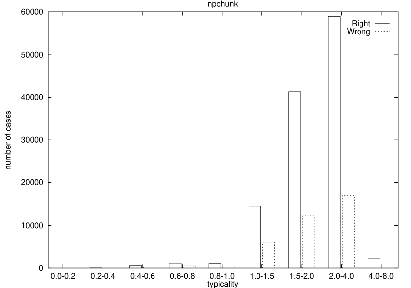
Figure 6: Histograms per typicality (left) and class-prediction strength (right) of the neighbors present in support sets for each of the four tasks. For each range (indicated at the $x$-axes), the number of instances leading to a correct classification (Right), and to a misclassification (Wrong), is displayed as a bar.

6.2 Properties of learning algorithms

If we classify instance $X$ by looking at its nearest neighbors, we are in fact estimating the probability $P(class|X)$, by looking at the relative frequency of the class in the set defined by $sim_{k}(X)$, where $sim_{k}(X)$ is a function from $X$ to the set of most similar instances present in the training data. The $sim_{k}(X)$ function given by the overlap metric groups varying numbers of instances into buckets of equal similarity. A bucket is defined by a particular number of mismatches with respect to instance $X$. Each bucket can further be decomposed into a number of schemata characterized by the position of the mismatch.

The search for the nearest neighbors results in the use of the most similar instantiated schema or bucket for extrapolation. In statistical language modeling this is known as backed-off estimation [Collins and Brooks,1995, Katz,1987]. The distance metric defines a specific-to-general ordering ($X\prec Y$: read $X$ is more specific than $Y$, see also [Zavrel and Daelemans,1997]), where the most specific schema is the schema with zero mismatches (i.e., an identical instance in memory), and the most general schema has a mismatch on every feature, which corresponds to the entire memory being retrieved.

If information gain weights are used in combination with the overlap metric, individual schemata instead of buckets become the steps of the back-off sequence (unless two schemata are exactly tied in their IG values). The $\prec$ ordering becomes slightly more complicated now, as it depends on the number of wild-cards and on the magnitude of the weights attached to those wild-cards. Let $S$ be the most specific (zero mismatches) schema. We can then define the $\prec$ ordering between schemata in the following equation, where $\Delta(X,Y)$ is the distance as defined in Equation 1.

$$S^{\prime}\prec S^{\prime\prime}\ \Leftrightarrow\ \Delta(S,S^{\prime})<\Delta(S,S^{\prime\prime})$$ (9)

This approach represents a type of implicit parallelism. The importance of all of the $2^{F}$ schemata is specified using only $F$ parameters (i.e., the IG weights), where $F$ is the number of features. Moreover, using the schemata keeps the information from all training instances available for extrapolation in those cases where more specific information is not available.

Decision trees can also be described as backed-off estimators of the class probability conditioned on the combination of the features-values. However, here some schemata are not available for extrapolation. Even in a decision tree without any pruning, such abstraction takes place. Once a test instance matches an arc with a certain value for a particular feature, the set of schemata from which it can receive a classification is restricted to those for which that feature matches. This means that other schemata which are more specific when judged by the ordering of Equation 9, are unavailable. If pruning is applied, even more schemata are blocked.

Figure 7: Percentage correct for our data sets plotted as a function of distance between the test instance and its nearest neighbor. The distances are normalized between zero and one, and discretized into a maximum of ten evenly spaced intervals to make a comparison across data sets possible.

Figure 7 shows why this elimination of schemata can be harmful. In this figure the percentage correct for our data sets is plotted as a function of specificity. The decrease of the accuracy seen in the graph clearly confirms the intuition that an extrapolation from a more specific support set is more likely to be correct. Reasoning in the other direction, it suggests that any forgetting of specific information from the training set will push at least some test instances in the direction of a less specific support set, and thus of lower accuracy.

	Average IG Overlap Distance (number of instances)
Task	FF			FT			TF			TT
	ib1	igt	n	ib1	igt	n	ib1	igt	n	ib1	igt	n
gs	0.03	0.05	(4083)	0.08	0.14	(249)	0.10	0.19	(552)	0.01	0.02	(62633)
pos	0.18	0.23	(1876)	0.26	0.37	(440)	0.27	0.40	(524)	0.07	0.08	(101776)
pp	0.06	0.07	(275)	0.06	0.08	(111)	0.06	0.07	(184)	0.05	0.06	(1820)
np	0.12	0.19	(343)	0.14	0.24	(160)	0.14	0.26	(324)	0.08	0.15	(24286)

Table 9: The average distance at which classification takes place for ib1-ig (listed under ib1) and igtree (listed under igt). The distances have been split out into four conditions: FF, FT, TF, and TT; the first letter refers to ib1-ig giving a False or True answer, the second refers in the same manner to the output of igtree. The third column gives the number of instances for that condition. The igtree distances have been computed from an unpruned tree.

A more direct illustration of this matter can be given for the limited accessibility of schemata in igtree. As the ordering of features is constant throughout the tree, the schemas that are accessible at any given node in the tree are limited to those that match all features with a higher ig weight. The depth of the igtree node at which classification was performed can directly be translated into a distance between the test pattern and the branch of the tree, using the ig weights. To make the comparison fair, we have used an unpruned igtree. Table 9 shows the average distances at which classifications were made for the four tasks at hand. igtree consistently classifies at a larger average distance than ib1-ig. Moreover, through analysis of those test instances that were misclassified by igtree, but classified correctly by ib1-ig (i.e., TF in Table 9), we found that for a majority (69% for gs, 90% for pos, 55% for pp, and 100% for np) of these instances the classification distance was larger for igtree than for ib1-ig. This means that in all these cases a closer neighbor was available to support a correct classification, but was not used, because its schema was not accesible.

6.2.1 Increasing $k$

As an aside, we note that we have reported solely on experiments with ib1-ig with $k=1$. Although it is not directly related to “forgetting”, taking a larger value of $k$ can also be considered as a type of abstraction, because the class is estimated from a somewhat smoothed region of the instance space. Only on the basis of the results described so far, we cannot claim that $k=1$ is the optimal setting for our experiments. The results discussed above suggest that the average ‘$k$’ actually surrounding an instance is larger than $1$, although many instances have only one or no friendly neighbor, especially in the case of the gs task. The latter suggests that a considerable amount of ambiguity is found in instances that are highly similar; matching with $k>1$ may fail to detect those cases in which an instance has one best-matching friendly neighbor, and many next-best-matching instances of a different class.

	Generalization accuracy (%)
Task	$k=1$	$k=2$	$k=3$	$k=5$
gs	93.45 $\pm$ 0.15	93.00 $\pm$ 0.15	92.71 $\pm$ 0.13	92.30 $\pm$ 0.12
pos	97.86 $\pm$ 0.05	97.72 $\pm$ 0.05	97.27 $\pm$ 0.04	95.91 $\pm$ 0.05
pp	83.48 $\pm$ 1.16	78.10 $\pm$ 1.26	75.19 $\pm$ 1.75	75.67 $\pm$ 1.53
np	98.07 $\pm$ 0.05	98.05 $\pm$ 0.05	98.23 $\pm$ 0.07	98.15 $\pm$ 0.09

Table 10: Generalization accuracies (in terms of percentages of correctly classified test instances) on the gs, pos, pp, and np tasks, by ib1-ig with $k=1$, 2, 3, and 5.

We performed experiments with ib1-ig on the four tasks with $k=2$, $k=3$, and $k=5$, and mostly found a decrease in generalization accuracy. Table 10 lists the effects of the higher values of $k$. For all tasks except np, setting $k>1$ leads to a harmful abstraction from the best-matching instance(s) to a more smoothed best matching group of instances.

In this Section, we have tried to interpret our empirical results in terms of properties of the data and of the learning algorithms used. A salient characteristic of our language learning tasks, shown most clearly in the gs data set but also present in the other data sets, is the presence of a high degree of class polymorphism (high disjunctivity). In many cases, these small disjuncts constitute productive (pockets of) exceptions which are useful in producing accurate extrapolations to new data. ib1-ig, through its implicit parallelism and its feature relevance weighting, is better suited than decision tree methods to make available the most specific relevant patterns in memory to extrapolate from.

7 Related research

[Daelemans,1995] provides an overview of memory-based learning work on phonological and morphological tasks (grapheme-to-phoneme conversion, syllabification, hyphenation, morphological synthesis, word stress assignment) at Tilburg University and the University of Antwerp in the early nineties. The present paper directly builds on the results obtained in that research. More recently, the approach has been applied to part-of-speech tagging (morphosyntactic disambiguation), morphological analysis, and the resolution of structural ambiguity (prepositional-phrase attachment) [Daelemans and Van den Bosch,1996, Van den Bosch, Daelemans, and Weijters,1996, Zavrel, Daelemans, and Veenstra,1997]. Whenever these studies involve a comparison of memory-based learning to more eager methods, a clear advantage of memory-based learning is reported.

Cardie [Cardie,1993, Cardie,1994] suggests a memory-based learning approach for both (morpho)syntactic and semantic disambiguation and shows excellent results compared to alternative approaches. [Ng and Lee,1996] report results superior to previous statistical methods when applying a memory-based learning method to word sense disambiguation. In reaction to [Mooney,1996] where it was shown that naive Bayes performed better than memory-based learning, [Ng,1997] showed that with higher values of $k$, memory-based learning obtained the same results as naive Bayes.

The exemplar-based reasoning aspects of memory-based learning are also prominent in the large literature on example-based machine translation (cf. [Jones,1996] for an overview), although systematic comparisons to eager approaches seem to be lacking in that field.

In the recent literature on statistical language learning, which currently still largely adheres to the hypothesis that what is exceptional (improbable) is unimportant, similar results as those discussed here for machine learning have been reported. In [Bod,1995], a data-oriented approach to parsing is described in which a treebank is used as a ‘memory’ and in which the parse of a new sentence is computed by reconstruction from subtrees present in the treebank. It is shown that removing all hapaxes (unique subtrees) from memory degrades generalization performance from 96% to 92%. Bod notes that “this seems to contradict the fact that probabilities based on sparse data are not reliable.” ([Bod,1995], p.68). In the same vein, [Collins and Brooks,1995] show that when applying the back-off estimation technique [Katz,1987] to learning prepositional-phrase attachment, removing all events with a frequency of less than 5 degrades generalization performance from 84.1% to 81.6%. In [Dagan, Lee, and Pereira,1997], finally, a similarity-based estimation method is compared to back-off and maximum-likelihood estimation on a pseudo-word sense disambiguation task. Again, a positive effect of events with frequency 1 in the training set on generalization accuracy is noted.

In the context of statistical language learning, it is also relevant to note that as far as comparable results are available, statistical techniques, which also abstract from exceptional events, never obtain a higher generalization accuracy than ib1-ig [Daelemans,1995, Zavrel and Daelemans,1997, Zavrel, Daelemans, and Veenstra,1997]. Reliable comparisons (in the sense of methods being compared on the same train and test data) with the empirical results reported here cannot be made, however.

In the machine learning literature, the problem of small disjuncts in concept learning has been studied before by [Quinlan,1991], who proposed more accurate error estimation methods for small disjuncts, and by [Holte, Acker, and Porter,1989]. The latter define a small disjunct as one that has small coverage (i.e., a small number of training items are correctly classified by it). This definition differs from ours, in which small disjuncts are those that have few neighbors with the same category. Nevertheless, similar phenomena are noted: sometimes small disjuncts constitute a significant portion of an induced definition, and it is hard to distinguish productive small disjuncts from noise (see also [Danyluk and Provost,1993]). A maximum-specificity bias for small disjuncts is proposed to make small disjuncts less error-prone. Memory-based learning is of course a good way of implementing this remedy (as noted, e.g., in [Aha,1992]). This prompted [Ting,1994b] to propose a composite learner with an instance-based component for small disjuncts, and a decision tree component for large disjuncts. This hybrid learner improves upon the c4.5 baseline for several definitions of ‘small disjunct’ for most of the data sets studied. Similar results have recently been reported by [Domingos,1996], where rise, a unification of rule induction (c4.5) and instance-based learning (pebls) is proposed. In an empirical study, rise turned out to be better than alternative approaches, including its two ‘parent’ algorithms. The fact that rule induction in rise is specific-to-general (starting by collapsing instances) rather than general-to-specific (as in the decision tree methods used in this paper), may make it a useful approach for our language data as well.

8 Conclusion and future research

We have provided empirical evidence for the hypothesis that forgetting exceptional instances, either by editing them away according to some exceptionality criterion in memory-based learning or by abstracting from them in decision-tree learning, is harmful to generalization accuracy in language learning. Although we found some exceptions to this hypothesis, the fact that abstraction or editing is never beneficial to generalization accuracy is consistently shown in all our experiments.

Data sets representing nlp tasks show a high degree of polymorphism: categories are represented in instance space as small regions with the same category separated by instances with a different category (the categories are highly disjunctive). This was empirically shown by looking at the average number of friendly neighbors per instance; an indirect measure of the average size of the homogeneous regions in instance space. This analysis showed that for our nlp tasks, classes are scattered across many disjunctive clusters in instance space. This turned out to be the case especially for the gs data set, the only task presented here which has extensively been studied in the ML literature before (through the similar nettalk data set). It will be necessary to investigate polymorphism further using more language data sets and more ways of operationalizing the concept of ‘small disjuncts’.

The high disjunctivity explains why editing the training set in memory-based learning using typicality and cps criteria does not improve generalization accuracy, and even tends to decrease it. The instances used for correct classification (what we called the support set) are as likely to be low-typical or low-class-prediction-strength (thus exceptional) instances as high-typical or high-class-prediction-strength instances. The editing that we find to be the most harmless (although never beneficial) to generalization accuracy is editing up to about 20% high-typical and high-class-prediction-strength instances. Nevertheless, these results leave room for combining memory-based learning and specific-to-general rule learning of the kind presented in [Domingos,1996]. It would be interesting further research to test his approach on our data.

The fact that the generalization accuracies of the decision-tree learning algorithms c5.0 and igtree are mostly worse than those of ib1-ig on this type of data set can be further explained by their properties. Interpreted as statistical backed-off estimators of the class probability given the feature-value vector, due to the way the information-theoretic splitting criterion works, some schemata (sets of partially matching instances) are not accessible for extrapolation in decision tree learning. Given the high disjunctivity of categories in language learning, abstracting away from these schemata and not using them for extrapolation is harmful. This type of abstraction takes place even when no pruning is used. Apparently, the assumption in decision tree learning that differences in relative importance of features can always be exploited is, for the tasks studied, untrue. Memory-based learning, on the other hand, because it implicitly keeps all schemes available for extrapolation, can use the advantages of information-theoretic feature relevance weighting without the disadvantages of losing relevant information. We plan to expand on the encouraging results on other data sets using tribl, a hybrid of igtree and ib1-ig that leaves schemas accesible when there is no clear feature-relevance distinction [Daelemans, Van den Bosch, and Zavrel,1997].

When decision trees are pruned, implying further abstraction from the training data, low-frequency instances with deviating classifications constitute the first information to be removed from memory. When the data representing a task is highly disjunctive, and instances do not represent noise but simply low-frequency instances that may (and do) reoccur in test data, as is especially the case with the gs task, pruning is harmful to generalization. The first reason for decision-tree learning to be harmful (accesability of schemata) is the most serious one, since it suggests that there is no parameter setting that may help c5.0 and similar algorithms in surpassing or equaling the performance of ib1-ig in these tasks. The second reason (pruning), less important than the first, only applies to data sets with low noise. However, there exist variations of decision tree learning that may not suffer from these problems (e.g., the lazy decision trees of [Friedman, Kohavi, and Yun,1996]) and that remain to be investigated in the context of our data.

Taken together, the empirical results of our research strongly suggest that keeping full memory of all training instances is at all times a good idea in language learning.

Acknowledgements

This research was done in the context of the “Induction of Linguistic Knowledge” research programme, supported partially by the Foundation for Language Speech and Logic (TSL), which is funded by the Netherlands Organization for Scientific Research (NWO). AvdB performed part of his work at the Department of Computer Science of the Universiteit Maastricht. The authors wish to thank Jorn Veenstra for his earlier work on the PP attachment and NP chunking data sets, and the other members of the Tilburg ILK group, Ton Weijters, Eric Postma, Jaap van den Herik, and the MLJ reviewers for valuable discussions and comments.

References

- [Abney,1991] Abney, S. 1991. Parsing by chunks. In Principle-Based Parsing. Kluwer Academic Publishers, Dordrecht.
- [Aha,1992] Aha, D. W. 1992. Generalizing from case studies: a case study. In Proceedings of the Ninth International Conference on Machine Learning, pages 1–10, San Mateo, CA. Morgan Kaufmann.
- [Aha,1997] Aha, D. W. 1997. Lazy learning: Special issue editorial. Artificial Intelligence Review, 11:7–10.
- [Aha, Kibler, and Albert,1991] Aha, D. W., D. Kibler, and M. Albert. 1991. Instance-based learning algorithms. Machine Learning, 6:37–66.
- [Atkeson, Moore, and Schaal,1997] Atkeson, C., A. Moore, and S. Schaal. 1997. Locally weighted learning. Artificial Intelligence Review, 11(1–5):11–73.
- [Baayen, Piepenbrock, and van Rijn,1993] Baayen, R. H., R. Piepenbrock, and H. van Rijn. 1993. The CELEX lexical data base on CD-ROM. Linguistic Data Consortium, Philadelphia, PA.
- [Bod,1995] Bod, R. 1995. Enriching linguistics with statistics: Performance models of natural language. Dissertation, ILLC, Universiteit van Amsterdam.
- [Cardie,1993] Cardie, C. 1993. A case-based approach to knowledge acquisition for domain-specific sentence analysis. In AAAI-93, pages 798–803.
- [Cardie,1994] Cardie, C. 1994. Domain Specific Knowledge Acquisition for Conceptual Sentence Analysis. Ph.D. thesis, University of Massachusets, Amherst, MA.
- [Cardie,1996] Cardie, C. 1996. Automatic feature set selection for case-based learning of linguistic knowledge. In Proc. of Conference on Empirical Methods in NLP. University of Pennsylvania.
- [Church,1988] Church, K. W. 1988. A stochastic parts program and noun phrase parser for unrestricted text. In Proc. of Second Applied NLP (ACL).
- [Collins and Brooks,1995] Collins, M.J and J. Brooks. 1995. Prepositional phrase attachment through a backed-off model. In Proc. of Third Workshop on Very Large Corpora, Cambridge.
- [Cost and Salzberg,1993] Cost, S. and S. Salzberg. 1993. A weighted nearest neighbour algorithm for learning with symbolic features. Machine Learning, 10:57–78.
- [Cover and Hart,1967] Cover, T. M. and P. E. Hart. 1967. Nearest neighbor pattern classification. Institute of Electrical and Electronics Engineers Transactions on Information Theory, 13:21–27.
- [Daelemans,1995] Daelemans, W. 1995. Memory-based lexical acquisition and processing. In P. Steffens, editor, Machine Translation and the Lexicon, volume 898 of Lecture Notes in Artificial Intelligence. Springer-Verlag, Berlin, pages 85–98.
- [Daelemans,1996] Daelemans, W. 1996. Experience-driven language acquisition and processing. In T. Van der Avoird and C. Corsius, editors, Proceedings of the CLS Opening Academic Year 1996-1997. CLS, Tilburg, pages 83–95.
- [Daelemans and Van den Bosch,1992] Daelemans, W. and A. Van den Bosch. 1992. Generalisation performance of backpropagation learning on a syllabification task. In M. F. J. Drossaers and A. Nijholt, editors, Proc. of TWLT3: Connectionism and Natural Language Processing, pages 27–37, Enschede. Twente University.
- [Daelemans and Van den Bosch,1996] Daelemans, W. and A. Van den Bosch. 1996. Language-independent data-oriented grapheme-to-phoneme conversion. In J. P. H. Van Santen, R. W. Sproat, J. P. Olive, and J. Hirschberg, editors, Progress in Speech Processing. Springer-Verlag, Berlin, pages 77–89.
- [Daelemans, Van den Bosch, and Weijters,1997] Daelemans, W., A. Van den Bosch, and A. Weijters. 1997. igtree: using trees for compression and classification in lazy learning algorithms. Artificial Intelligence Review, 11:407–423.
- [Daelemans, Van den Bosch, and Zavrel,1997] Daelemans, W., A. Van den Bosch, and J. Zavrel. 1997. A feature-relevance heuristic for indexing and compressing large case bases. In M. Van Someren and G. Widmer, editors, Poster Papers of the Ninth European Conference on Machine Learing, pages 29–38, Prague, Czech Republic. University of Economics.
- [Daelemans et al.,1996] Daelemans, W., J. Zavrel, P. Berck, and S. Gillis. 1996. MBT: A memory-based part of speech tagger generator. In E. Ejerhed and I.Dagan, editors, Proc. of Fourth Workshop on Very Large Corpora, pages 14–27. ACL SIGDAT.
- [Daelemans et al.,1998] Daelemans, W., J. Zavrel, K. Van der Sloot, and A. Van den Bosch. 1998. TiMBL: Tilburg Memory-Based Learner, version 1.0, reference guide. Technical report, ILK 98-03, Tilburg, The Netherlands.
- [Dagan, Lee, and Pereira,1997] Dagan, I., L. Lee, and F. Pereira. 1997. Similarity-based methods for word sense disambiguation. In Proceedings of the 35th ACL and the 8th EACL, Madrid, Spain, pages 56–63.
- [Danyluk and Provost,1993] Danyluk, A. P. and F. J. Provost. 1993. Small disjuncts in action: learning to diagnose errors in the local loop of the telephone network. In Proceedings of the Tenth International Conference on Machine Learning, pages 81–88, San Mateo, CA. Morgan Kaufmann.
- [Devijver and Kittler,1980] Devijver, P. A. and J. Kittler. 1980. On the edited nearest neighbor rule. In Proceedings of the Fifth International Conference on Pattern Recognition. The Institute of Electrical and Electronics Engineers.
- [Devijver and Kittler,1982] Devijver, P. .A. and J. Kittler. 1982. Pattern recognition. A statistical approach. Prentice-Hall, London, UK.
- [Dietterich,1998 in press] Dietterich, T. G. 1998 (in press). Approximate statistical tests for comparing supervised classification learning algorithms. Neural Computation.
- [Dietterich, Hild, and Bakiri,1995] Dietterich, T. G., H. Hild, and G. Bakiri. 1995. A comparison of id3 and backpropagation for English text-to-speech mapping. Machine Learning, 19(1):5–28.
- [Domingos,1996] Domingos, P. 1996. Unifying instance-based and rule-based induction. Machine Learning, 24:141–168.
- [Friedman, Kohavi, and Yun,1996] Friedman, J. H., R. Kohavi, and Y. Yun. 1996. Lazy decision trees. In Proceedings of the Thirteenth National Conference on Artificial Intelligence, pages 717–724, Cambridge, MA. The MIT Press.
- [Hart,1968] Hart, P. E. 1968. The condensed nearest neighbor rule. IEEE Transactions on Information Theory, 14:515–516.
- [Holte, Acker, and Porter,1989] Holte, R. C., L. E. Acker, and B. W. Porter. 1989. Concept learning and the problem of small disjuncts. In Proceedings of the Eleventh International Joint Conference on Artificial Intelligence, pages 813–818, San Mateo, CA. Morgan Kaufmann.
- [Jones,1996] Jones, D. 1996. Analogical natural language processing. UCL Press, London, UK.
- [Katz,1987] Katz, S. M. 1987. Estimation of probabilities from sparse data for the language model component of a speech recognizer. IEEE Transactions on Acoustics, Speech and Signal Processing, ASSP-35:400–401, March.
- [Kolodner,1993] Kolodner, J. 1993. Case-based reasoning. Morgan Kaufmann, San Mateo, CA.
- [Lehnert,1987] Lehnert, W. 1987. Case-based problem solving with a large knowledge base of learned cases. In Proceedings of the Sixth National Conference on Artificial Intelligence (AAAI-87), pages 301–306, Los Altos, CA. Morgan Kaufmann.
- [Magerman,1994] Magerman, D. M. 1994. Natural language parsing as statistical pattern recognition. Dissertation, Stanford University.
- [Marcus, Santorini, and Marcinkiewicz,1993] Marcus, M., B. Santorini, and M.A. Marcinkiewicz. 1993. Building a large annotated corpus of english: The penn treebank. Computational Linguistics, 19(2):313–330.
- [Markovitch and Scott,1988] Markovitch, S. and P. D. Scott. 1988. The role of forgetting in learning. In Proceedings of the Fifth International Conference on Machine Learning, pages 459–465, Ann Arbor, MI. Morgan Kaufmann.
- [Michie, Spiegelhalter, and Taylor,1994] Michie, D., D.J. Spiegelhalter, and C.C. Taylor. 1994. Machine learning, neural and statistical classification. Ellis Horwood, New York.
- [Mooney,1996] Mooney, R. J. 1996. Comparative experiments on disambiguating word senses: An illustration of the role of bias in machine learning. In Proceedings of the Conference on Empirical Methods in Natural Language Processing, EMNLP, pages 82–91.
- [Mooney and Califf,1995] Mooney, R. J. and M. E. Califf. 1995. Induction of first-order decision lists: Results on learning the past tense of english verbs. Journal of Artificial Intelligence Research, 3:1–24.
- [Ng,1997] Ng, H. T. 1997. Exemplar-based word sense disambiguation: some recent improvements. In Proceedings of the Second Conference on Empirical Methods in Natural Language Processing, pages 208–213.
- [Ng and Lee,1996] Ng, H. T. and H. B. Lee. 1996. Intergrating multiple knowledge sources to disambiguate word sense: An exemplar-based approach. In Proc. of 34th meeting of the Assiociation for Computational Linguistics.
- [Quinlan,1991] Quinlan, J. R. 1991. Improved estimation for the accuracy of small disjuncts. Machine Learning, 6:93–98.
- [Quinlan,1986] Quinlan, J.R. 1986. Induction of Decision Trees. Machine Learning, 1:81–206.
- [Quinlan,1993] Quinlan, J.R. 1993. c4.5: Programs for Machine Learning. Morgan Kaufmann, San Mateo, CA.
- [Ramshaw and Marcus,1995] Ramshaw, L.A. and M.P. Marcus. 1995. Text chunking using transformation-based learning. In Proc. of third workshop on very large corpora, pages 82–94, June.
- [Ratnaparkhi,1997] Ratnaparkhi, A. 1997. A linear observed time statistical parser based on maximum entropy models. In Proceedings of the Second Conference on Empirical Methods in Natural Language Processing, EMNLP, pages 1–10.
- [Ratnaparkhi, Reynar, and Roukos,1994] Ratnaparkhi, A., J. Reynar, and S. Roukos. 1994. A maximum entropy model for prepositional phrase attachment. In Workshop on Human Language Technology, Plainsboro, NJ, March. ARPA.
- [Rosch and Mervis,1975] Rosch, E. and C. B. Mervis. 1975. Family resemblances: studies in the internal structure of categories. Cognitive Psychology, 7:573–605.
- [Salganicoff,1993] Salganicoff, M. 1993. Density-adaptive learning and forgetting. In Proceedings of the Fifth International Conference on Machine Learning, pages 276–283, Amherst, MA. Morgan Kaufmann.
- [Salzberg,1990] Salzberg, S. 1990. Learning with nested generalised exemplars. Kluwer Academic Publishers, Norwell, MA.
- [Sejnowski and Rosenberg,1987] Sejnowski, T. J. and C. S. Rosenberg. 1987. Parallel networks that learn to pronounce English text. Complex Systems, 1:145–168.
- [Shavlik, Mooney, and Towell,1991] Shavlik, J. W., R. J. Mooney, and G. G. Towell. 1991. An experimental comparison of symbolic and connectionist learning algorithms. Machine Learning, 6:111–143.
- [Stanfill,1987] Stanfill, C. 1987. Memory-based reasoning applied to English pronunciation. In Proceedings of the Sixth National Conference on Artificial Intelligence (aaai-87), pages 577–581, Los Altos, CA. Morgan Kaufmann.
- [Stanfill and Waltz,1986] Stanfill, C. and D. Waltz. 1986. Toward memory-based reasoning. Communications of the acm, 29(12):1213–1228, December.
- [Ting,1994a] Ting, K. M. 1994a. The problem of atypicality in instance-based learning. In Proceedings of the The Third Pacific Rim International Conference on Artificial Intelligence, pages 360–366.
- [Ting,1994b] Ting, K. M. 1994b. The problem of small disjuncts: Its remedy in decision trees. In Proceedings of the Tenth Canadian Conference on Artificial Intelligence, pages 91–97.
- [Van den Bosch, Daelemans, and Weijters,1996] Van den Bosch, A., W. Daelemans, and A. Weijters. 1996. Morphological analysis as classification: an inductive-learning approach. In K. Oflazer and H. Somers, editors, Proceedings of the Second International Conference on New Methods in Natural Language Processing, NeMLaP-2, Ankara, Turkey, pages 79–89.
- [Van den Bosch et al.,1995] Van den Bosch, A., A. Weijters, H. J. Van den Herik, and W. Daelemans. 1995. The profit of learning exceptions. In Proceedings of the 5th Belgian-Dutch Conference on Machine Learning, pages 118–126.
- [Voisin and Devijver,1987] Voisin, J. and P. A. Devijver. 1987. An application of the Multiedit-Condensing technique to the reference selection problem in a print recognition system. Pattern Recognition, 5:465–474.
- [Weiss and Kulikowski,1991] Weiss, S. and C. Kulikowski. 1991. Computer systems that learn. San Mateo, CA: Morgan Kaufmann.
- [Wilson,1972] Wilson, D. 1972. Asymptotic properties of nearest neighbor rules using edited data. Institute of Electrical and Electronic Engineers Transactions on Systems, Man and Cybernetics, 2:408–421.
- [Wolpert,1989] Wolpert, D. 1989. Constructing a generalizer superior to NETtalk via mathematical theory of generalization. Neural Networks, 3:445–452.
- [Zavrel and Daelemans,1997] Zavrel, J. and W. Daelemans. 1997. Memory-based learning: Using similarity for smoothing. In Proc. of 35th annual meeting of the ACL, Madrid.
- [Zavrel, Daelemans, and Veenstra,1997] Zavrel, J., W. Daelemans, and J. Veenstra. 1997. Resolving pp attachment ambiguities with memory-based learning. In M. Ellison, editor, Proc. of the Workshop on Computational Language Learning (CoNLL’97), ACL, Madrid.
- [Zhang,1992] Zhang, J. 1992. Selecting typical instances in instance-based learning. In Proceedings of the International Machine Learning Conference 1992, pages 470–479.