The Essence of Constraint Propagation

Abstract

We show that several constraint propagation algorithms (also called (local) consistency, consistency enforcing, Waltz, filtering or narrowing algorithms) are instances of algorithms that deal with chaotic iteration. To this end we propose a simple abstract framework that allows us to classify and compare these algorithms and to establish in a uniform way their basic properties.

Note. This is a full, revised version of our article “From Chaotic Iteration to Constraint Propagation”, Proc. of 24th International Colloquium on Automata, Languages and Programming (ICALP ’97), (invited lecture), Springer-Verlag Lecture Notes in Computer Science 1256, pp. 36-55, (1997).

Keywords: constraint propagation, chaotic iteration, generic algorithms.

1 Introduction

1.1 Motivation

Over the last ten years constraint programming emerged as an interesting and viable approach to programming. In this approach the programming process is limited to a generation of requirements (“constraints”) and a solution of these requirements by means of general and domain specific methods. The techniques useful for finding solutions to sets of constraints were studied for some twenty years in the field of Constraint Satisfaction. One of the most important of them is constraint propagation, a process of reducing a constraint satisfaction problem to another one that is equivalent but “simpler”.

The algorithms that achieve such a reduction usually aim at reaching some “local consistency”, which denotes some property approximating in some loose sense “global consistency”, which is the consistency of the whole constraint satisfaction problem. In fact, most of the notions of local consistency are neither implied by nor imply global consistency (for a simple illustration of this statement see, e.g., Example 11 in Subsection 3.3).

For some constraint satisfaction problems such an enforcement of local consistency is already sufficient for finding a solution in an efficient way or for determining that none exists. In some other cases this process substantially reduces the size of the search space which makes it possible to solve the original problem more efficiently by means of some search algorithm.

The aim of this paper is to show that the constraint propagation algorithms (also called (local) consistency, consistency enforcing, Waltz, filtering or narrowing algorithms) can be naturally explained by means of chaotic iteration, a basic technique used for computing limits of iterations of finite sets of functions that originated from numerical analysis (see, e.g., Chazan and Miranker [8]) and was adapted for computer science needs by Cousot and Cousot [11].

In our presentation we study chaotic iteration of monotonic and inflationary functions on partial orders first. This is done in Section 2. Then, in Section 3 we show how specific constraint propagation algorithms can be obtained by choosing specific functions and specific partial orders.

This two-step presentation reveals that several constraint propagation algorithms proposed in the literature are instances of generic chaotic iteration algorithms studied here.

The adopted framework allows us to prove properties of these algorithms in a simple, uniform way. This clarifies which properties of the so-called reduction functions (also called relaxation rules or narrowing functions) account for correctness of these algorithms. For example, it turns out that idempotence is not needed here. Further, this framework allows us to separate an analysis of general properties, such as termination and independence of the scheduling strategy, from consideration of specific, constraint-related properties, such as equivalence. Even the consequences of choosing a queue instead of a set for scheduling purposes can be already clarified without introducing constraints.

We also explain how by characterizing a given notion of a local consistency as a common fixed point of a finite set of monotonic and inflationary functions we can automatically generate an algorithm achieving this notion of consistency by “feeding” these functions into a generic chaotic iteration algorithm. By studying these functions in separation we can also compare specific constraint propagation algorithms.

A recent work of Monfroy and Réty [22] also shows how this approach makes it possible to derive generic distributed constraint propagation algorithms in a uniform way.

Several general presentations of constraint propagation algorithms have been published before. In Section 4 we explain how our work relates to and generalizes the work of others.

1.2 Preliminaries

Definition 1

Consider a sequence of domains ${\cal D}:=D_{1},\mbox{$\ldots$},D_{n}$.

• By a scheme (on $n$) we mean a sequence of different elements from $[1..n]$.

• We say that $C$ is a constraint (on ${\cal D}$) with scheme $i_{1},\mbox{$\ldots$},i_{l}$ if $C\mbox{$\>\subseteq\>$}D_{i_{1}}\times\cdots\times D_{i_{l}}$.

• Let ${\bf s}:=s_{1},\mbox{$\ldots$},s_{k}$ be a sequence of schemes. We say that a sequence of constraints $C_{1},\mbox{$\ldots$},C_{k}$ on ${\cal D}$ is an s-sequence if each $C_{i}$ is with scheme $s_{i}$.

• By a Constraint Satisfaction Problem $\langle\cal D;\cal C\rangle$, in short CSP, we mean a sequence of domains ${\cal D}$ together with an s-sequence of constraints ${\cal C}$ on ${\cal D}$. We call then s the scheme of $\langle\cal D;\cal C\rangle$. $\Box$

In principle a constraint can have more than one scheme, for example when all domains are equal. This eventuality should not cause any problems in the sequel. Given an $n$-tuple $d:=d_{1},\mbox{$\ldots$},d_{n}$ in $D_{1}\times\cdots\times D_{n}$ and a scheme $s:=i_{1},\mbox{$\ldots$},i_{l}$ on $n$ we denote by $d[s]$ the tuple $d_{i_{1}},\mbox{$\ldots$},d_{i_{l}}$. In particular, for $j\in[1..n]$  $d[j]$ is the $j$-th element of $d$. By a solution to a CSP $\langle\cal D;\cal C\rangle$, where ${\cal D}:=D_{1},\mbox{$\ldots$},D_{n}$, we mean an $n$-tuple $d\in D_{1}\times\cdots\times D_{n}$ such that for each constraint $C$ in ${\cal C}$ with scheme $s$ we have $d[s]\in C$.

Consider now a sequence of schemes $s_{1},\mbox{$\ldots$},s_{k}$. By its union, written as $\langle s_{1},\mbox{$\ldots$},s_{k}\rangle$ we mean the scheme obtained from the sequences $s_{1},\mbox{$\ldots$},s_{k}$ by removing from each $s_{i}$ the elements present in some $s_{j}$, where $j<i$, and by concatenating the resulting sequences. For example, $\langle(3,7,2),(4,3,7,5),(3,5,8)\rangle=(3,7,2,4,5,8)$. Recall that for an $s_{1},\mbox{$\ldots$},s_{k}$-sequence of constraints $C_{1},\mbox{$\ldots$},C_{k}$ their join, written as $C_{1}\Join\cdots\Join C_{k}$, is defined as the constraint with scheme $\langle s_{1},\mbox{$\ldots$},s_{k}\rangle$ and such that

$$d\in C_{1}\Join\cdots\Join C_{k}\mbox{ iff $d[s_{i}]\in C_{i}$ for $i\in[1..k]$}.$$

Further, given a constraint $C$ and a subsequence $s$ of its scheme, we denote by $\Pi_{s}(C)$ the constraint with scheme $s$ defined by

$$\Pi_{s}(C):=\mbox{$\{{d[s]\mid d\in C}\}$},$$

and call it the projection of $C$ on $s$. In particular, for a constraint $C$ with scheme $s$ and an element $j$ of $s$, $\Pi_{j}(C)=\mbox{$\{{a\mid\mbox{$\exists$}d\in C\>a=d[j]}\}$}$.

Given a CSP $\langle\cal D;\cal C\rangle$ we denote by $Sol(\langle\cal D;\cal C\rangle)$ the set of all solutions to it. If the domains are clear from the context we drop the reference to $\cal D$ and just write $Sol({\cal C})$. The following observation is useful.

Note 1

Consider a CSP $\langle\cal D;\cal C\rangle$ with ${\cal D}:=D_{1},\mbox{$\ldots$},D_{n}$ and ${\cal C}:=C_{1},\mbox{$\ldots$},C_{k}$ and with scheme s.

1. 
   

   $$Sol(\langle{\cal D};{\cal C}\rangle)=C_{1}\Join\cdots\Join C_{k}\Join_{i\in I}D_{i},$$

   where $I:=\mbox{$\{{i\in[1..n]\mid\mbox{ $i$ {\rm does not appear in {\bf s}}}}\}$}$.

2. For every s-subsequence C of ${\cal C}$ and $d\in Sol(\langle{\cal D};{\cal C}\rangle)$ we have $d[\langle{\bf s}\rangle]\in Sol({\bf C})$.

   $\Box$

Finally, we call two CSP’s equivalent if they have the same set of solutions. Note that we do not insist that these CSP’s have the same sequence of domains or the same scheme.

2 Chaotic Iterations

In our study of constraint propagation we proceed in two stages. In this section we study chaotic iterations of functions on partial orders. Then in the next section we explain how this framework can be readily used to explain constraint propagation algorithms.

2.1 Chaotic Iterations on Simple Domains

In general, chaotic iterations are defined for functions that are projections on individual components of a specific function with several arguments. In our approach we study a more elementary situation in which the functions are unrelated but satisfy certain properties. We need the following concepts.

Definition 2

Consider a set $D$, an element $d\in D$ and a set of functions $F:=\mbox{$\{{f_{1},\mbox{$\ldots$},f_{k}}\}$}$ on $D$.

• By a run (of the functions $f_{1},\mbox{$\ldots$},f_{k}$) we mean an infinite sequence of numbers from $[1..k]$.

• A run $i_{1},i_{2},\mbox{$\ldots$}$ is called fair if every $i\in[1..k]$ appears in it infinitely often.

• By an iteration of $F$ associated with a run $i_{1},i_{2},\mbox{$\ldots$}$ and starting with $d$ we mean an infinite sequence of values $d_{0},d_{1},\mbox{$\ldots$}$ defined inductively by

  $$d_{0}:=d,$$

  $$d_{j}:=f_{i_{j}}(d_{j-1}).$$

  When $d$ is the least element of $D$ in some partial order clear from the context, we drop the reference to $d$ and talk about an iteration of $F$.

• An iteration of $F$ is called chaotic if it is associated with a fair run. $\Box$

Definition 3

Consider a partial order $(D,\mbox{$\ \sqsubseteq\ $})$. A function $f$ on $D$ is called

• inflationary if $x\mbox{$\ \sqsubseteq\ $}f(x)$ for all $x$,

• monotonic if $x\mbox{$\ \sqsubseteq\ $}y$ implies $f(x)\mbox{$\ \sqsubseteq\ $}f(y)$ for all $x,y$,

• idempotent if $f(f(x))=f(x)$ for all $x$. $\Box$

In what follows we study chaotic iterations on specific partial orders.

Definition 4

We call a partial order $(D,\mbox{$\ \sqsubseteq\ $})$ an $\sqcup$-po if

• $D$ contains the least element, denoted by $\bot$,

• for every increasing sequence

  $$d_{0}\>\mbox{$\ \sqsubseteq\ $}\>d_{1}\>\mbox{$\ \sqsubseteq\ $}\>d_{2}\>\mbox{$\ldots$}$$

  of elements from $D$, the least upper bound of the set

  $$\mbox{$\{{d_{0},\>d_{1},\>d_{2},\mbox{$\ldots$}}\}$},$$

  denoted by $\bigsqcup_{n=0}^{\infty}d_{n}$ and called the limit of $d_{0},d_{1},\mbox{$\ldots$}$, exists,

• for all $a,b\in D$ the least upper bound of the set $\{{a,b}\}$, denoted by $a\sqcup b$, exists.

Further, we say that

• an increasing sequence $d_{0}\>\mbox{$\ \sqsubseteq\ $}\>d_{1}\>\mbox{$\ \sqsubseteq\ $}\>d_{2}\>\mbox{$\ldots$}$ eventually stabilizes at d if for some $j\geq 0$ we have $d_{i}=d$ for $i\geq j$,

• a partial order satisfies the finite chain property if every increasing sequence of its elements eventually stabilizes. $\Box$

Intuitively, $\bot$ is an element with the least amount of information and $a\sqsubseteq b$ means that $b$ contains more information than $a$. Clearly, the second condition of the definition of $\sqcup$-po is automatically satisfied if $D$ is finite.

It is also clear that $\sqcup$-po’s are closed under the Cartesian product. In the applications we shall use specific $\sqcup$-po’s built out of sets and their Cartesian products.

Definition 5

Let $D$ be a set. We say that a family ${\cal F}(D)$ of subsets of $D$ is based on $D$ if

• $D\in{\cal F}(D)$,

• for every decreasing sequence

  $$X_{0}\supseteq X_{1}\supseteq X_{2}\mbox{$\ldots$}$$

  of elements of ${\cal F}(D)$

  $$\cap^{\infty}_{i=0}X_{i}\in{\cal F}(D),$$

• for all $X,Y\in{\cal F}(D)$ we have $X\cap Y\in{\cal F}(D)$.

That is, a set ${\cal F}(D)$ of subsets of $D$ is based on $D$ iff ${\cal F}(D)$ with the relation $\ \sqsubseteq\$ defined by

$$X\sqsubseteq Y\mbox{ iff }X\supseteq Y$$

is an $\sqcup$-po. In this $\sqcup$-po $\bot=D$ and $X\sqcup Y=X\cap Y$. We call $({\cal F}(D),\sqsubseteq)$ an $\sqcup$-po based on $D$. $\Box$

The following two examples of families of subsets based on a domain will be used in the sequel.

Example 1

Define

$${\cal F}(D):={\cal P}(D),$$

that is ${\cal F}(D)$ consists of all subsets of $D$. This family of subsets will be used to discuss general constraint propagation algorithms. $\Box$

Example 2

Let $(D,\mbox{$\ \sqsubseteq\ $})$ be a partial order with the $\ \sqsubseteq\$-least element min, the $\ \sqsubseteq\$-greatest element max and such that for every two elements $a,b\in D$ both $a\sqcup b$ and $a\sqcap b$ exists.

Examples of such partial orders are a linear order with the $\ \sqsubseteq\$-least element and the $\ \sqsubseteq\$-greatest element and the set of all subsets of a given set with the subset relation.

Given two elements $a,b$ of $D$ define

$$[a,b]:=\mbox{$\{{c\mid a\leq c\mbox{ and }c\leq b}\}$}$$

and call such a set an interval. So for $b<a$ we have $[a,b]=\mbox{$\emptyset$}$, for $b=a$ we have $[a,b]=\mbox{$\{{a}\}$}$ and $[{\em min}..{\em max}]=D$.

Let now $F$ be a finite subset of $D$ containing min and max. Define

$${\cal F}(D):=\mbox{$\{{[a,b]\mid a,b\in F}\}$},$$

that is ${\cal F}(D)$ consists of all intervals with the bounds in $F$. Note that ${\cal F}(D)$ is indeed a family of subsets based on $D$ since

• $D=[{\em min}..{\em max}]$,

• ${\cal F}(D)$ is finite, so every decreasing sequence of elements of ${\cal F}(D)$ eventually stabilizes,

• for $a,b,c,d\in F$ we have

  $$[a,b]\cap[c,d]=[a\sqcup c,b\sqcap d].$$

Such families of subsets will be used to discuss constraint propagation algorithms on reals. In these applications $D$ will be the set of real numbers augmented with $-\infty$ and $+\infty$ and $F$ the set of floating point numbers. $\Box$

The following observation can be easily distilled from a more general result due to Cousot and Cousot [11]. To keep the paper self-contained we provide a direct proof.

Theorem 2.1 ((Chaotic Iteration))

Consider an $\sqcup$-po $(D,\mbox{$\ \sqsubseteq\ $})$ and a set of functions $F:=\mbox{$\{{f_{1},\mbox{$\ldots$},f_{k}}\}$}$ on $D$. Suppose that all functions in $F$ are inflationary and monotonic. Then the limit of every chaotic iteration of $F$ exists and coincides with

$$\bigsqcup_{j=0}^{\infty}f\uparrow j,$$

where the function $f$ on $D$ is defined by:

$$f(x):=\bigsqcup_{i=1}^{k}f_{i}(x)$$

and $f\uparrow j$ is an abbreviation for $f^{j}(\bot)$, the $j$-th fold iteration of $f$ started at $\bot$.

Proof. First, notice that $f$ is inflationary, so $\bigsqcup_{j=0}^{\infty}f\uparrow j$ exists. Fix a chaotic iteration $d_{0},d_{1},\mbox{$\ldots$}$ of $F$ associated with a fair run $i_{1},i_{2},\mbox{$\ldots$}$. Since all functions $f_{i}$ are inflationary, $\bigsqcup_{j=0}^{\infty}d_{j}$ exists. The result follows directly from the following two claims.

Claim 1

$\mbox{$\forall$}j\>\mbox{$\exists$}m\>f\uparrow j\mbox{$\ \sqsubseteq\ $}d_{m}$.

Proof. We proceed by induction on $j$.

Base. $j=0$. As $f\uparrow 0=\bot=d_{0}$, the claim is obvious.

Induction step. Assume that for some $j\geq 0$ we have $f\uparrow j\mbox{$\ \sqsubseteq\ $}d_{m}$ for some $m\geq 0$. Since

$$f\uparrow(j+1)=f(f\uparrow j)=\bigsqcup_{i=1}^{k}f_{i}(f\uparrow j),$$

it suffices to prove

$$\mbox{$\forall$}i\in[1..k]\>\mbox{$\exists$}m_{i}\>f_{i}(f\uparrow j)\mbox{$\ \sqsubseteq\ $}d_{m_{i}}.$$ (1)

Indeed, we have then by the fact that $d_{l}\mbox{$\ \sqsubseteq\ $}d_{l+1}$ for $l\geq 0$

$$\bigsqcup_{i=1}^{k}f_{i}(f\uparrow j)\mbox{$\ \sqsubseteq\ $}\bigsqcup_{i=1}^{k}d_{m_{i}}\mbox{$\ \sqsubseteq\ $}d_{m^{\prime}}$$

where $m^{\prime}:=max\mbox{$\{{m_{i}\mid i\in[1..k]}\}$}$.

So fix $i\in[1..k]$. By fairness of the considered run $i_{1},i_{2},\mbox{$\ldots$}$, for some $m_{i}>m$ we have $i_{m_{i}}=i$. Then $d_{m_{i}}=f_{i}(d_{m_{i}-1})$. Now $d_{m}\mbox{$\ \sqsubseteq\ $}d_{m_{i}-1}$, so by the monotonicity of $f_{i}$ we have

$$f_{i}(f\uparrow j)\mbox{$\ \sqsubseteq\ $}f_{i}(d_{m})\mbox{$\ \sqsubseteq\ $}f_{i}(d_{m_{i}-1})=d_{m_{i}}.$$

This proves (1). $\Box$

Claim 2

$\mbox{$\forall$}m\>d_{m}\mbox{$\ \sqsubseteq\ $}f\uparrow m$.

Proof. The proof is by a straightforward induction on $m$. Indeed, for $m=0$ we have $d_{0}=\bot=f\uparrow 0$, so the induction base holds.

To prove the induction step suppose that for some $m\geq 0$ we have $d_{m}\mbox{$\ \sqsubseteq\ $}f\uparrow m$. For some $i\in[1..k]$ we have $d_{m+1}=f_{i}(d_{m})$, so by the monotonicity of $f$ we get $d_{m+1}=f_{i}(d_{m})\mbox{$\ \sqsubseteq\ $}f(d_{m})\mbox{$\ \sqsubseteq\ $}f(f\uparrow m)=f\uparrow(m+1).$ $\Box$

$\Box$

In many situations some chaotic iteration studied in the Chaotic Iteration Theorem 2.1 eventually stabilizes. This is for example the case when $(D,\mbox{$\ \sqsubseteq\ $})$ satisfies the finite chain property. In such cases the limit of every chaotic iteration can be characterized in an alternative way.

Corollary 1 ((Stabilization))

Suppose that under the assumptions of the Chaotic Iteration Theorem 2.1 some chaotic iteration of $F$ eventually stabilizes. Then every chaotic iteration of $F$ eventually stabilizes at the least fixed point of $f$.

Proof. It suffices to note that if some chaotic iteration $d_{0},d_{1}\mbox{$\ldots$}$ of $F$ eventually stabilizes at some $d_{m}$ then by Claims 1 and 2 $f\uparrow m=d_{m}$, so

$$\bigsqcup_{j=0}^{\infty}f\uparrow j=f\uparrow m.$$ (2)

Then, again by Claims 1 and 2, every chaotic iteration of $F$ stabilizes at $f\uparrow m$ and it is easy to see that by virtue of (2) $f\uparrow m$ is the least fixed point of $f$. $\Box$

Finally, using the above results we can compare chaotic iterations resulting from different sets of functions.

Corollary 2 ((Comparison))

Consider an $\sqcup$-po $(D,\mbox{$\ \sqsubseteq\ $})$ and two set of functions, $F:=\mbox{$\{{f_{1},\mbox{$\ldots$},f_{k}}\}$}$ and $G:=\mbox{$\{{g_{1},\mbox{$\ldots$},g_{l}}\}$}$ on $D$. Suppose that all functions in $F$ and $G$ are inflationary and monotonic. Further, assume that for $i\in[1..k]$ there exist $j_{1},\mbox{$\ldots$},j_{m}\in[1..l]$ such that

$$f_{i}(x)\mbox{$\ \sqsubseteq\ $}g_{j_{1}}\circ\mbox{$\ldots$}\circ g_{j_{m}}(x)\mbox{ for all $x$.}$$

Then $lim(F)\mbox{$\ \sqsubseteq\ $}lim(G)$ for the uniquely defined limits $lim(F)$ and $lim(G)$ of the chaotic iterations of $F$ and $G$.

Proof. Straightforward using the Chaotic Iteration Theorem 2.1 and the fact that the functions in $G$ are inflationary. $\Box$

2.2 Chaotic Iterations on Compound Domains

Not much more can be deduced about the process of the chaotic iteration unless the structure of the domain $D$ is further known. So assume now that $\sqcup$-po $(D,\mbox{$\ \sqsubseteq\ $})$ is the Cartesian product of the $\sqcup$-po’s $(D_{i},\mbox{$\ \sqsubseteq\ $}_{i})$, for $i\in[1..n]$. In what follows we consider a modification of the situation studied in the Chaotic Iteration Theorem 2.1 in which each function $f_{i}$ affects only certain components of $D$.

Consider the partial orders $(D_{i},\mbox{$\ \sqsubseteq\ $}_{i})$, for $i\in[1..n]$ and a scheme $s:=i_{1},\mbox{$\ldots$},i_{l}$ on $n$. Then by $(D_{s},\mbox{$\ \sqsubseteq\ $}_{s})$ we mean the Cartesian product of the partial orders $(D_{i_{j}},\mbox{$\ \sqsubseteq\ $}_{i_{j}})$, for $j\in[1..l]$.

Given a function $f$ on $D_{s}$ we say that $f$ is with scheme $s$. Instead of defining iterations for the case of the functions with schemes, we rather reduce the situation to the one studied in the previous subsection. To this end we canonically extend each function $f$ on $D_{s}$ to a function $f^{+}$ on $D$ as follows. Suppose that $s=i_{1},\mbox{$\ldots$},i_{l}$ and

$$f(d_{i_{1}},\mbox{$\ldots$},d_{i_{l}})=(e^{\prime}_{i_{1}},\mbox{$\ldots$},e^{\prime}_{i_{l}}).$$

Let for $j\in[1..n]$

$$e_{j}:=\left\{\begin{array}[]{ll}e^{\prime}_{j}&\mbox{if $j$ is an element of $s$},\\ d_{j}&\mbox{otherwise. }\end{array}\right.$$

Then we set

$$f^{+}(d_{1},\mbox{$\ldots$},d_{n}):=(e_{1},\mbox{$\ldots$},e_{n}).$$

Suppose now that $(D,\mbox{$\ \sqsubseteq\ $})$ is the Cartesian product of the $\sqcup$-po’s $(D_{i},\mbox{$\ \sqsubseteq\ $}_{i})$, for $i\in[1..n]$, and $F:=\mbox{$\{{f_{1},\mbox{$\ldots$},f_{k}}\}$}$ is a set of functions with schemes that are all inflationary and monotonic. Then the following algorithm can be used to compute the limit of the chaotic iterations of $F^{+}:=\mbox{$\{{f^{+}_{1},\mbox{$\ldots$},f^{+}_{k}}\}$}$. We say here that a function $f$ depends on $i$ if $i$ is an element of its scheme.

Generic Chaotic Iteration Algorithm (CI)

$d:=\underbrace{(\bot,\mbox{$\ldots$},\bot)}_{\mbox{$n$ times}}$;

$d^{\prime}:=d$;

$G:=F$;

while $G\neq\mbox{$\emptyset$}$ do

choose $g\in G$; suppose $g$ is with scheme $s$;

$G:=G-\mbox{$\{{g}\}$}$;

$d^{\prime}[s]:=g(d[s])$;

if $d[s]\neq d^{\prime}[s]$ then

$G:=G\cup\mbox{$\{{f\in F\mid\mbox{$f$ depends on some }i\mbox{ in $s$ such that }d[i]\neq d^{\prime}[i]}\}$}$;

$d[s]:=d^{\prime}[s]$

fi

od

Obviously, the condition $d[s]\neq d^{\prime}[s]$ can be omitted here. We retained it to keep the form of the algorithm more intuitive.

The following observation will be useful in the proof of correctness of this algorithm.

Note 2

Consider the partial orders $(D_{i},\mbox{$\ \sqsubseteq\ $}_{i})$, for $i\in[1..n]$, a scheme $s$ on $n$ and a function $f$ with scheme $s$. Then

1. $f$ is inflationary iff $f^{+}$ is.

2. $f$ is monotonic iff $f^{+}$ is. $\Box$

Observe that, in spite of the name of the algorithm, its infinite executions do not need to correspond to chaotic iterations. The following example will be of use for a number of different purposes.

Example 3

Consider the set of natural numbers $\cal N$ augmented with $\omega$, with the order $\leq$. In this order $k\leq\omega$ for $k\in{\cal N}$. Next, we consider the following three functions on ${\cal N}\cup\mbox{$\{{\omega}\}$}$:

$$f_{1}(n):=\left\{\begin{array}[]{ll}n+1&\mbox{if $n$ is even},\\ n&\mbox{if $n$ is odd},\\ \omega&\mbox{if $n$ is $\omega$, }\end{array}\right.$$

$$f_{2}(n):=\left\{\begin{array}[]{ll}n+1&\mbox{if $n$ is odd},\\ n&\mbox{if $n$ is even},\\ \omega&\mbox{if $n$ is $\omega$, }\end{array}\right.$$

$$f_{3}(n):=\omega.$$

Clearly, the underlying order is an $\sqcup$-po and the functions $f_{1},f_{2}$ and $f_{3}$ are all inflationary, monotonic and idempotent. Now, there is an infinite execution of the CI algorithm that corresponds with the run $1,2,1,2,\mbox{$\ldots$}$. This execution does not correspond to any chaotic iteration of $\{{f_{1},f_{2},f_{3}}\}$. $\Box$

However, when we focus on terminating executions we obtain the following result in the proof of which our analysis of chaotic iterations is of help.

Theorem 2.2 ((CI))

1. Every terminating execution of the CI algorithm computes in $d$ the least fixed point of the function $f$ on $D$ defined by

   $$f(x):=\bigsqcup_{i=1}^{k}f^{+}_{i}(x).$$

2. If all $(D_{i},\mbox{$\ \sqsubseteq\ $}_{i})$, where $i\in[1..n]$, satisfy the finite chain property, then every execution of the CI algorithm terminates.

Proof. It is simpler to reason about a modified, but equivalent, algorithm in which the assignments $d^{\prime}[s]:=g(d[s])$ and $d[s]:=d^{\prime}[s]$ are respectively replaced by $d^{\prime}:=g^{+}(d)$ and $d:=d^{\prime}$ and the test $d[s]\neq d^{\prime}[s]$ by $d\neq d^{\prime}$.

$(i)$ Note that the formula

$$I:=\mbox{$\forall$}f\in F-G\>f^{+}(d)=d$$

is an invariant of the while loop of the modified algorithm. Thus upon its termination

$$(G=\mbox{$\emptyset$})\mbox{$\ \wedge\ $}I$$

holds, that is

$$\mbox{$\forall$}f\in F\>f^{+}(d)=d.$$

Consequently, some chaotic iteration of $F^{+}$ eventually stabilizes at $d$. Hence $d$ is the least fixpoint of the function $f$ defined in item $(i)$ because the Stabilization Corollary 1 is applicable here by virtue of Note 2.

$(ii)$ Consider the lexicographic order of the partial orders $(D,\sqsupseteq)$ and $({\cal N},\leq)$, defined on the elements of $D\times{\cal N}$ by

$$(d_{1},n_{1})\leq_{lex}(d_{2},n_{2})\ {\rm iff}\ d_{1}\sqsupset d_{2}\ {\rm or}\ (d_{1}=d_{2}\ {\rm and}\ n_{1}\leq n_{2}).$$

We use here the inverse order $\sqsupset$ defined by: $d_{1}\sqsupset d_{2}$ iff $d_{2}\sqsubseteq d_{1}$ and $d_{2}\neq d_{1}$.

By Note 2(i) all functions $f^{+}_{i}$ are inflationary, so with each while loop iteration of the modified algorithm the pair

$$(d,card\>G)$$

strictly decreases in this order $\leq_{lex}$. However, in general the lexicographic order $(D\times{\cal N},\leq_{lex})$ is not well-founded and in fact termination is not guaranteed. But assume now additionally that each partial order $(D_{i},\mbox{$\ \sqsubseteq\ $}_{i})$ satisfies the finite chain property. Then so does their Cartesian product $(D,\mbox{$\ \sqsubseteq\ $})$. This means that $(D,\sqsupseteq)$ is well-founded and consequently so is $(D\times{\cal N},\leq_{lex})$ which implies termination. $\Box$

When all considered functions $f_{i}$ are also idempotent, we can reverse the order of the two assignments to $G$, that is to put the assignment $G:=G-\mbox{$\{{g}\}$}$ after the if-then-fi statement, because after applying an idempotent function there is no use in applying it immediately again. Let us denote by CII the algorithm resulting from this movement of the assignment $G:=G-\mbox{$\{{g}\}$}$.

More specialized versions of the CI and CII algorithms can be obtained by representing $G$ as a queue. To this end we use the operation ${\bf enqueue}(F,Q)$ which for a set $F$ and a queue $Q$ enqueues in an arbitrary order all the elements of $F$ in $Q$, denote the empty queue by empty, and the head and the tail of a non-empty queue $Q$ respectively by ${\bf head}(Q)$ and ${\bf tail}(Q)$. The following algorithm is then a counterpart of the CI algorithm.

Generic Chaotic Iteration Algorithm with a Queue (CIQ)

$d:=\underbrace{(\bot,\mbox{$\ldots$},\bot)}_{\mbox{$n$ times}}$;

$d^{\prime}:=d$;

$Q:={\bf empty}$;

${\bf enqueue}(F,Q)$;

while $Q\neq{\bf empty}$ do

$g:={\bf head}(Q)$; suppose $g$ is with scheme $s$;

$Q:={\bf tail}(Q)$;

$d^{\prime}[s]:=g(d[s])$;

if $d[s]\neq d^{\prime}[s]$ then

${\bf enqueue}(\mbox{$\{{f\in F\mid\mbox{$f$ depends on some }i\mbox{ in $s$ such that }d[i]\neq d^{\prime}[i]}\}$},Q)$;

$d[s]:=d^{\prime}[s]$

fi

od

Denote by CIIQ the modification of the CIQ algorithm that is appropriate for the idempotent functions, so the one in which the assignment $Q:={\bf tail}(Q)$ is performed after the if-then-fi statement.

It is easy to see that the claims of the CI Theorem 2.2 also hold for the CII, CIQ and CIIQ algorithms. A natural question arises whether for the specialized versions CIQ and CIIQ some additional properties can be established. The answer is positive. We need an auxiliary notion and a result first.

Definition 6

Consider a set of functions $F:=\mbox{$\{{f_{1},\mbox{$\ldots$},f_{k}}\}$}$ on a domain $D$.

• We say that an element $i\in[1..k]$ is eventually irrelevant for an iteration $d_{0},d_{1},\mbox{$\ldots$}$ of $F$ if $\mbox{$\exists$}m\geq 0\>\mbox{$\forall$}j\geq m\>f_{i}(d_{j})=d_{j}$.

• An iteration of $F$ is called semi-chaotic if every $i\in[1..k]$ that appears finitely often in its run is eventually irrelevant for this iteration. $\Box$

So every chaotic iteration is semi-chaotic but not conversely.

Note 3

1. Every semi-chaotic iteration $\xi$ corresponds to a chaotic iteration $\xi^{\prime}$ with the same limit as $\xi$ and such that $\xi$ eventually stabilizes at some $d$ iff $\xi^{\prime}$ does.

2. Every infinite execution of the CIQ (respectively CIIQ) algorithm corresponds to a semi-chaotic iteration.

Proof. 
(i) $\xi$ can be transformed into the desired chaotic iteration $\xi^{\prime}$ by repeating from a certain moment on some elements of it.

(ii) Consider an infinite execution of the CIQ algorithm. Let $i_{1},i_{2},\mbox{$\ldots$}$ be the run associated with it and $\xi:=d_{0},d_{1},\mbox{$\ldots$}$ the iteration of $F^{+}$ associated with this run.

Consider the set $A$ of the elements of $[1..k]$ that appear finitely often in the run $i_{1},i_{2},\mbox{$\ldots$}$. For some $m\geq 0$ we have $i_{j}\not\in A$ for $j>m$. This means by the structure of this algorithm that after $m$ iterations of the while loop no function $f_{i}$ with $i\in A$ is ever present in the queue $Q$.

By virtue of the invariant $I$ used in the proof of the CI Theorem 2.2 we then have $f^{+}_{i}(d_{j})=d_{j}$ for $i\in A$ and $j\geq m$. This proves that $\xi$ is semi-chaotic.

The proof for the CIIQ algorithm is the same. $\Box$

Item (i) shows that the results of Subsection 2.1 can be strengthened to semi-chaotic iterations. However, the property of being a semi-chaotic iteration cannot be determined from the run only. So, for simplicity, we decided to limit our exposition to chaotic iterations. Next, it is easy to show that item (ii) cannot be strengthened to chaotic iterations.

We can now prove the desired results. The first one shows that the nondeterminism present in the CIQ and CIIQ algorithms has no bearing on their termination.

Theorem 2.3 ((Termination))

If some execution of the CIQ (respectively CIIQ) algorithm terminates, then all executions of the CIQ (respectively CIIQ) algorithm terminate.

Proof. We concentrate on the CIQ algorithm. For the CIIQ algorithm the proof is the same.

Consider a terminating execution of the CIQ algorithm. Construct a chaotic iteration of $F^{+}$ the initial prefix of which corresponds with this execution. By virtue of the invariant $I$ this iteration eventually stabilizes. By the Stabilization Corollary 1

every chaotic iteration of $$F^{+}$$ eventually stabilizes. (3)

Suppose now by contradiction that some execution of the CIQ algorithm does not terminate. Let $\xi$ be the iteration of $F^{+}$ associated with this execution. By the structure of this algorithm

$$\xi$$ does not eventually stabilize. (4)

By Note 3(ii) $\xi$ is a semi-chaotic iteration. Consider a chaotic iteration $\xi^{\prime}$ of $F^{+}$ that corresponds with $\xi$ by virtue of Note 3(i). We conclude by (4) that $\xi^{\prime}$ does not eventually stabilize. This contradicts (3). $\Box$

So for a given Cartesian product $(D,\mbox{$\ \sqsubseteq\ $})$ of the $\sqcup$-po’s and a finite set $F$ of inflationary, monotonic and idempotent functions either all executions of the CIQ (respectively CIIQ) algorithm terminate or all of them are infinite. In the latter case we can be more specific.

Theorem 2.4 ((Non-termination))

For every infinite execution of the CIQ (respectively CIIQ) algorithm the limit of the corresponding iteration of $F$ exists and coincides with

$$\bigsqcup_{j=0}^{\infty}f\uparrow j,$$

where $f$ is defined as in the CI Theorem 2.2(i).

Proof. Consider an infinite execution of the CIQ algorithm. By Note 3(ii) it corresponds to a semi-chaotic iteration $\xi$ of $F^{+}$. By Note 3(i) $\xi$ corresponds to a chaotic iteration of $F^{+}$ with the same limit. The desired conclusion now follows by the Chaotic Iteration Theorem 2.1.

The proof for the CIIQ algorithm is the same. $\Box$

Neither of the above two results holds for the CI and CII algorithms. Indeed, take the $\sqcup$-po $({\cal N}\cup\mbox{$\{{\omega}\}$},\leq)$ and the functions $f_{1},f_{2},f_{3}$ of Example 3. Then clearly both infinite and finite executions of the CI and CII algorithms exist. We leave to the reader the task of modifying Example 3 in such a way that for both CI and CII algorithms infinite executions exist with different limits of the corresponding iterations.

3 Constraint Propagation

Let us return now to the study of CSP’s. We show here how the results of the previous section can be used to explain the constraint propagation process.

In general, two basic approaches fall under this name:

• reduce the constraints while maintaining equivalence;

• reduce the domains while maintaining equivalence.

3.1 Constraint Reduction

In each step of the constraint reduction process one or more constraints are replaced by smaller ones. In general, the smaller constraints are not arbitrary. For example, when studying linear constraints usually the smaller constraints are also linear.

To model this aspect of constraint reduction we associate with each CSP an $\sqcup$-po that consists of the CSP’s that can be generated during the constraint reduction process.

Because the domains are assumed to remain unchanged, we can identify each CSP with the sequence of its constraints. This leads us to the following notions.

Consider a CSP ${\cal P}:=\langle{\cal D};C_{1},\mbox{$\ldots$},C_{k}\rangle$. Let for $i\in[1..k]$ $({\cal F}(C_{i}),\supseteq)$ be an $\sqcup$-po based on $C_{i}$. We call the Cartesian product $(CO,\mbox{$\ \sqsubseteq\ $})$ of $({\cal F}(C_{i}),\supseteq)$, with $i\in[1..k]$, a constraint $\sqcup$-po associated with ${\cal P}$.

As in Subsection 2.2, for a scheme $s:=i_{1},\mbox{$\ldots$},i_{l}$ we denote by $(CO_{s},\mbox{$\ \sqsubseteq\ $}_{s})$ the Cartesian product of the partial orders $({\cal F}(C_{i_{j}}),\supseteq)$, where $j\in[1..l]$.

Note that $CO_{s}={\cal F}(C_{i_{1}})\times\cdots\times{\cal F}(C_{i_{l}})$. Because we want now to use constraints in our analysis and constraint are sets of tuples, we identify $CO_{s}$ with the set

$$\mbox{$\{{X_{1}\times\cdots\times X_{l}\mid\mbox{ $X_{j}\in{\cal F}(C_{i_{j}})$ for $j\in[1..l]$}}\}$}.$$

In this way we can write the elements of $CO_{s}$ as Cartesian products $X_{1}\times\cdots\times X_{l}$, so as (specific) sets of $l$-tuples, instead of as $(X_{1},\mbox{$\ldots$},X_{l})$, and similarly with $CO$.

Note that $C_{1}\times\cdots\times C_{k}$ is the $\ \sqsubseteq\$-least element of $CO$. Also, note that because of the use of the inverse subset order $\supseteq$ we have for $X_{1}\times\cdots\times X_{l}\in CO_{s}$ and $Y_{1}\times\cdots\times Y_{l}\in CO_{s}$

$X_{1}\times\cdots\times X_{l}\mbox{$\ \sqsubseteq\ $}_{s}Y_{1}\times\cdots\times Y_{l}$	iff	$X_{1}\times\cdots\times X_{l}\supseteq Y_{1}\times\cdots\times Y_{l}$
	(iff	$X_{i}\supseteq Y_{i}$ for $i\in[1..l]$),

$(X_{1}\times\cdots\times X_{l})\sqcup_{s}(Y_{1}\times\cdots\times Y_{l})$	=	$(X_{1}\times\cdots\times X_{l})\cap(Y_{1}\times\cdots\times Y_{l})$
	(=	$(X_{1}\cap Y_{1})\times\cdots\times(X_{l}\cap Y_{l}))$.

This allows us to use from now on the set theoretic counterparts $\supseteq$ and $\cap$ of $\mbox{$\ \sqsubseteq\ $}_{s}$ and $\sqcup_{s}$. Note that for the partial order $(CO_{s},\mbox{$\ \sqsubseteq\ $}_{s})$ a function $g$ on $CO_{s}$ is inflationary iff ${\bf C}\supseteq g({\bf C})$ and $g$ is monotonic iff it is monotonic w.r.t. the set inclusion.

So far we have introduced an $\sqcup$-po associated with a CSP. Next, we introduce functions by means of which chaotic iterations will be generated.

Definition 7

Consider a CSP $\langle{\cal D};C_{1},\mbox{$\ldots$},C_{k}\rangle$ together with a sequence of families of sets ${\cal F}(C_{i})$ based on $C_{i}$, for $i\in[1..k]$, and a scheme $s$ on $k$. By a constraint reduction function with scheme $s$ we mean a function $g$ on $CO_{s}$ such that for all ${\bf C}\in CO_{s}$

• ${\bf C}\supseteq g({\bf C})$,

• $Sol({\bf C})=Sol(g({\bf C}))$. $\Box$

C is here a Cartesian product of some constraints and in the second condition we identified it with the sequence of these constraints, and similarly with $g({\bf C})$. The first condition states that $g$ reduces the constraints $C_{i}$, where $i$ is an element of $s$, while the second condition states that during this constraint reduction process no solution to ${\bf C}$ is lost.

Example 4

As a first example of a constraint reduction function take ${\cal F}(C):={\cal P}(C)$ for each constraint $C$ and consider the following function $g$ on some $CO_{s}$:

$$g(C\times{\bf C}):=C^{\prime}\times{\bf C},$$

where $C^{\prime}=\Pi_{t}(Sol(C,{\bf C}))$ and $t$ is the scheme of $C$. In other words, $C^{\prime}$ is the projection of the set of solutions of $(C,{\bf C})$ on the scheme of $C$.

To see that $g$ is indeed a constraint reduction function, first note that by the definition of $Sol$ we have $C^{\prime}\mbox{$\>\subseteq\>$}C$, so $C\times{\bf C}\supseteq g(C\times{\bf C})$. Next, note that for $d\in Sol(C,{\bf C})$ we have $d[t]\in\Pi_{t}(Sol(C,{\bf C}))$, so $d\in Sol(C^{\prime},{\bf C})$. This implies that $Sol(C,{\bf C})=Sol(g(C,{\bf C})).$

Note also that $g$ is monotonic w.r.t. the set inclusion and idempotent. $\Box$

Example 5

As another example that is of importance for the discussion in Subsection 4.1 consider a CSP $\langle D_{1},\mbox{$\ldots$},D_{n};\cal C\rangle$ of binary constraints such that for each scheme $i,j$ on $n$ there is exactly one constraint, which we denote by $C_{i,j}$. Again put ${\cal F}(C):={\cal P}(C)$ for each constraint $C$.

Define now for each scheme $k,l,m$ on $n$ the following function $g^{m}_{k,l}$ on $CO_{s}$, where $s$ is the triple corresponding to the positions of the constraints $C_{k,l},C_{k,m}$ and $C_{m,l}$ in ${\cal C}$:

$$g^{m}_{k,l}(X_{k,l}\times X_{k,m}\times X_{m,l}):=(X_{k,l}\cap\Pi_{k,l}(X_{k,m}\Join X_{m,l}))\times X_{k,m}\times X_{m,l}.$$

To prove that the functions $g^{m}_{k,l}$ are constraint reduction functions it suffices to note that by simple properties of the $\Join$ operation and by Note 1(i) we have

$X_{k,l}\cap\Pi_{k,l}(X_{k,m}\Join X_{m,l})$	=	$\Pi_{k,l}(X_{k,l}\Join X_{k,m}\Join X_{m,l})$
	=	$\Pi_{k,l}(Sol(X_{k,l},X_{k,m},X_{m,l}))$,

so these functions are special cases of the functions defined in Example 4. $\Box$

Example 6

As a final example consider linear inequalities over integers. Let $x_{1},\mbox{$\ldots$},x_{n}$ be different variables ranging over integers, where $n>0$. By a linear inequality we mean here a formula of the form

$$\sum_{i=1}^{n}a_{i}x_{i}\leq b,$$

where $a_{1},\mbox{$\ldots$},a_{n}$ and $b$ are integers.

In what follows we consider CSP’s that consist of finite or countable sets of linear inequalities. Each such set determines a subset of ${\cal N}^{n}$ which we view as a single constraint. Call such a subset an INT-LIN set.

Fix now a constraint $C$ that is an INT-LIN set formed by a finite or countable set LI of linear inequalities. Define ${\cal F}(C)$ to be the set of INT-LIN sets formed by a finite or countable set of linear inequalities extending LI. Clearly, ${\cal F}(C)$ is a family of sets based on $C$.

Given now $m$ linear inequalities

$$\sum_{i=1}^{n}a^{j}_{i}x_{i}\leq b^{j},$$

where $j\in[1..m]$, and $m$ nonnegative reals $c_{1},\mbox{$\ldots$},c_{m}$, we construct a new linear inequality

$$\sum_{i=1}^{n}(\sum_{j=1}^{m}c_{j}a^{j}_{i})x_{i}\leq\sum_{j=1}^{m}c_{j}b^{j}.$$

If for $i\in[1..n]$ each coefficient $\sum_{j=1}^{m}c_{j}a^{j}_{i}$ is an integer, then we replace the right-hand side by $\lfloor\sum_{i=1}^{m}c_{j}b^{j}\rfloor$.

This yields the inequality

$$\sum_{i=1}^{n}(\sum_{j=1}^{m}c_{j}a^{j}_{i})x^{j}_{i}\leq\lfloor\sum_{j=1}^{m}c_{j}b^{j}\rfloor$$

that is called a Gomory-Chvátal cutting plane.

An addition of a cutting plane to a set of linear inequalities on integers maintains equivalence, so it is an example of a constraint reduction function.

It is well-known that the process of deriving cutting planes does not have to stop after one application (see, e.g., Cook, Cunningham, Pulleyblank, and Schrijver [9, Section 6.7]), so this reduction function is non-idempotent. $\Box$

We now show that when the constraint reduction function discussed in Example 4 is modified by applying it to each argument constraint simultaneously, it becomes a constraint reduction function that is in some sense optimal.

More precisely, assume the notation of Definition 8 and let $s:=i_{1},\mbox{$\ldots$},i_{l}$. Define a function $\rho$ on $CO_{s}$ as follows:

$$\rho({\bf C}):={\bf C}^{\prime},$$

where

$${\bf C}:=C_{i_{1}}\times\cdots\times C_{i_{l}},$$

$${\bf C}^{\prime}:=C^{\prime}_{i_{1}}\times\cdots\times C^{\prime}_{i_{l}},$$

with each $C^{\prime}_{i_{j}}:=\Pi_{t_{j}}(Sol({\bf C}))$, where $t_{j}$ is the scheme of $C_{i_{j}}$.

So $\rho({\bf C})$ replaces every constraint $C$ in C by the projection of $Sol({\bf C})$ on the scheme of $C$.

Note 4 ((Characterization))

Assume the notation of Definition 7. A function $g$ on $CO_{s}$ is a constraint reduction function iff for all ${\bf C}\in CO_{s}$

$$\rho({\bf C})\mbox{$\>\subseteq\>$}g({\bf C})\mbox{$\>\subseteq\>$}{\bf C}.$$

Proof. Suppose that $s:=i_{1},\mbox{$\ldots$},i_{l}$. We have the following string of equivalences for

$$g({\bf C}):=X_{i_{1}}\times\cdots\times X_{i_{l}}:$$

$\rho({\bf C})\mbox{$\>\subseteq\>$}g({\bf C})$ iff $\Pi_{t_{j}}(Sol({\bf C}))\mbox{$\>\subseteq\>$}X_{i_{j}}$ for $j\in[1..l]$ iff $Sol({\bf C})\mbox{$\>\subseteq\>$}Sol(g({\bf C}))$.

So $\rho({\bf C})\mbox{$\>\subseteq\>$}g({\bf C})\mbox{$\>\subseteq\>$}{\bf C}$ iff ($Sol({\bf C})=Sol(g({\bf C}))$ and $g({\bf C})\mbox{$\>\subseteq\>$}{\bf C}$). $\Box$

Take now a CSP ${\cal P}:=\langle{\cal D};C_{1},\mbox{$\ldots$},C_{k}\rangle$ and a sequence of constraints $C^{\prime}_{1},\mbox{$\ldots$},C^{\prime}_{k}$ such that $C^{\prime}_{i}\mbox{$\>\subseteq\>$}C_{i}$ for $i\in[1..k]$. Let ${\cal P}^{\prime}:=\langle{\cal D};C^{\prime}_{1},\mbox{$\ldots$},C^{\prime}_{k}\rangle$. We say then that ${\cal P^{\prime}}$ is determined by ${\cal P}$ and $C^{\prime}_{1}\times\cdots\times C^{\prime}_{k}$. Further, we say that ${\cal P^{\prime}}$ is smaller than ${\cal P^{\prime}}$ and ${\cal P}$ is larger than ${\cal P^{\prime}}$.

Consider now a CSP ${\cal P}:=\langle{\cal D};C_{1},\mbox{$\ldots$},C_{k}\rangle$ and a constraint reduction function $g$. Suppose that

$$g^{+}(C_{1}\times\cdots\times C_{k})=C^{\prime}_{1}\times\cdots\times C^{\prime}_{k},$$

where $g^{+}$ is the canonic extension of $g$ to $CO$ defined in Subsection 2.2. We now define

$$g({\cal P}):=\langle{\cal D};C^{\prime}_{1},\mbox{$\ldots$},C^{\prime}_{k}\rangle.$$

We have the following observation.

Lemma 1

Consider a CSP ${\cal P}$ and a constraint reduction function $g$. Then ${\cal P}$ and $g({\cal P})$ are equivalent.

Proof. Suppose that $s$ is the scheme of the function $g$ and let C be an element of $CO_{s}$. So C is a Cartesian product of some constraints. As before we identify it with the sequence of these constraints. For some sequence of schemes s,  C is the s-sequence of the constraints of ${\cal P}$.

Let now $d$ be a solution to ${\cal P}$. Then by Note 1(ii) we have $d[\langle{\bf s}\rangle]\in Sol({\bf C})$, so by the definition of $g$ also $d[\langle{\bf s}\rangle]\in Sol(g({\bf C}))$. Hence for every constraint $C^{\prime}$ in $g({\bf C})$ with scheme $s^{\prime}$ we have $d[s^{\prime}]\in C^{\prime}$ since $d[\langle{\bf s}\rangle][s^{\prime}]=d[s^{\prime}]$. So $d$ is a solution to $g({\cal P})$. The converse implication holds by the definition of a constraint reduction function. $\Box$

When dealing with a specific CSP with a constraint $\sqcup$-po associated with it we have in general several constraint reduction functions, each defined on a possibly different domain. To study the effect of their interaction we can use the Chaotic Iteration Theorem 2.1 in conjunction with the above Lemma. After translating the relevant notions into set theoretic terms we get the following direct consequence of these results. (In this translation $CO_{s}$ corresponds to $D_{s}$ and $CO$ to $D$.)

Theorem 3.1 ((Constraint Reduction))

Consider a CSP ${\cal P}:=\langle{\cal D};C_{1},\mbox{$\ldots$},C_{k}\rangle$ with a constraint $\sqcup$-po associated with it. Let $F:=\mbox{$\{{g_{1},\mbox{$\ldots$},g_{k}}\}$}$, where each $g_{i}$ is a constraint reduction function. Suppose that all functions $g_{i}$ are monotonic w.r.t. the set inclusion. Then

• the limit of every chaotic iteration of $F^{+}:=\mbox{$\{{g^{+}_{1},\mbox{$\ldots$},g^{+}_{k}}\}$}$ exists;

• this limit coincides with

  $$\bigcap_{j=0}^{\infty}g^{j}(C_{1}\times\cdots\times C_{k}),$$

  where the function $g$ on $CO$ is defined by:

  $$g({\bf C}):=\bigcap_{i=1}^{k}g^{+}_{i}({\bf C}),$$

• the CSP determined by ${\cal P}$ and this limit is equivalent to ${\cal P}$. $\Box$

Informally, this theorem states that the order of the applications of the constraint reduction functions does not matter, as long as none of them is indefinitely neglected. Moreover, the CSP corresponding to the limit of such an iteration process of the constraint reduction functions is equivalent to the original one.

Consider now a CSP ${\cal P}$ with a constraint $\sqcup$-po associated with it that satisfies the finite chain property. Then we can use the CI, CII, CIQ and CIIQ algorithms to compute the limits of the chaotic iterations considered in the above Theorem. We shall explain in Subsection 4.1 how by instantiating these algorithms with specific constraint $\sqcup$-po’s and constraint reduction functions we obtain specific algorithms considered in the literature.

In each case, by virtue of the CI Theorem 2.2 and its reformulations for the CII, CIQ and CIIQ algorithms, we can conclude that these algorithms compute the greatest common fixpoint w.r.t. the set inclusion of the functions from $F^{+}$. Consequently, the CSP determined by ${\cal P}$ and this limit is the largest CSP that is both smaller than ${\cal P}$ and is a fixpoint of the considered constraint reduction functions.

So the limit of the constraint propagation process could be added to the collection of important greatest fixpoints presented in Barwise and Moss [2].

3.2 Domain Reduction

In this subsection we study the domain reduction process. First, we associate with each CSP an $\sqcup$-po that “focuses” on the domain reduction.

Consider a CSP ${\cal P}:=\langle D_{1},\mbox{$\ldots$},D_{n};{\cal C}\rangle$. Let for $i\in[1..n]$ $({\cal F}(D_{i}),\supseteq)$ be an $\sqcup$-po based on $D_{i}$. We call the Cartesian product $(DO,\mbox{$\ \sqsubseteq\ $})$ of $({\cal F}(D_{i}),\supseteq)$, with $i\in[1..n]$ a domain $\sqcup$-po associated with ${\cal P}$.

As in Subsection 2.2, for a scheme $s:=i_{1},\mbox{$\ldots$},i_{l}$ we denote by $(DO_{s},\mbox{$\ \sqsubseteq\ $}_{s})$ the Cartesian product of the partial orders $({\cal F}(D_{i_{j}}),\supseteq)$, where $j\in[1..l]$. Then, as in the previous subsection, we identify $DO_{s}$ with the set

$$\mbox{$\{{X_{1}\times\cdots\times X_{l}\mid\mbox{ $X_{j}\in{\cal F}(D_{i_{j}})$ for $j\in[1..l]$}}\}$}.$$

Next, we introduce functions that reduce domains. These functions are associated with constraints. Constraints are arbitrary sets of $k$-tuples for some $k$, while the $\mbox{$\ \sqsubseteq\ $}_{s}$ order and the $\sqcup_{s}$ operation are defined only on Cartesian products. So to define these functions we use the set theoretic counterparts $\supseteq$ and $\cap$ of $\mbox{$\ \sqsubseteq\ $}_{s}$ and $\sqcup_{s}$ which are defined on arbitrary sets.

Definition 8

Consider a sequence of domains $D_{1},\mbox{$\ldots$},D_{n}$ together with a sequence of families of sets ${\cal F}(D_{i})$ based on $D_{i}$, for $i\in[1..n]$, and a scheme $s$ on $n$. By a domain reduction function for a constraint $C$ with scheme $s$ we mean a function $f$ on $DO_{s}$ such that for all ${\bf D}\in DO_{s}$

• ${\bf D}\supseteq f({\bf D})$,

• $C\cap{\bf D}=C\cap f({\bf D})$. $\Box$

The first condition states that $f$ reduces the “current” domains associated with the constraint $C$ (so no solution to $C$ is “gained”), while the second condition states that during this domain reduction process no solution to $C$ is “lost”. In particular, the second condition implies that if $C\mbox{$\>\subseteq\>$}{\bf D}$ then $C\mbox{$\>\subseteq\>$}f({\bf D})$.

Example 7

As a simple example of a domain reduction functions consider a binary constraint $C\mbox{$\>\subseteq\>$}D_{1}\times D_{2}$. Let ${\cal F}(D_{i}):={\cal P}(D_{i})$ with $i\in[1,2]$ be the families of sets based on $D_{1}$ and $D_{2}$.

Define now the projection functions $\pi_{1}$ and $\pi_{2}$ on $DO_{1,2}={\cal P}(D_{1})\times{\cal P}(D_{2})$ as follows:

$$\pi_{1}(X\times Y):=X^{\prime}\times Y,$$

where $X^{\prime}=\mbox{$\{{a\in X\mid\mbox{$\exists$}b\in Y\>(a,b)\in C}\}$}$, and

$$\pi_{2}(X\times Y):=X\times Y^{\prime},$$

where $Y^{\prime}=\mbox{$\{{b\in Y\mid\mbox{$\exists$}a\in X\>(a,b)\in C}\}$}$. It is straightforward to check that $\pi_{1}$ and $\pi_{2}$ are indeed domain reduction functions. Further, these functions are monotonic w.r.t. the set inclusion and idempotent. $\Box$

Example 8

As another example of a domain reduction function consider an $n$-ary constraint $C\mbox{$\>\subseteq\>$}D_{1}\times\cdots\times D_{n}$. Let for $i\in[1..n]$ the family of sets based on $D_{i}$ be defined by ${\cal F}(D_{i}):={\cal P}(D_{i})$.

Note that $DO={\cal P}(D_{1})\times\cdots\times{\cal P}(D_{n})$. Define now the projection function $\pi_{C}$ by putting for ${\bf D}\in DO$

$$\pi_{C}({\bf D}):=\Pi_{1}(C\cap{\bf D})\times\cdots\times\Pi_{n}(C\cap{\bf D}).$$

Recall from Subsection 1.2 that $\Pi_{i}(C\cap{\bf D})=\mbox{$\{{a\mid\mbox{$\exists$}d\in C\cap{\bf D}\ a=d[i]}\}$}$. Clearly $\pi_{C}$ is a domain reduction function for $C$ and is monotonic w.r.t. the set inclusion and idempotent.

Here the scheme of $C$ is $1,\mbox{$\ldots$},n$. Obviously, $\pi_{C}$ can be defined in an analogous way for a constraint $C$ with an arbitrary scheme. $\Box$

So all three domain reduction functions deal with projections, respectively on the first, second or all components and can be visualized by means of Figure 1.

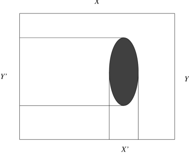
Figure 1: Domain reduction functions.

The following observation provides an equivalent definition of a domain reduction function in terms of the projection function defined in the last example.

Note 5 ((Characterization))

Assume the notation of Definition 8. A function $f$ on $DO_{s}$ is a domain reduction function for the constraint $C$ iff for all ${\bf D}\in DO_{s}$

$$\pi_{C}({\bf D})\mbox{$\>\subseteq\>$}f({\bf D})\mbox{$\>\subseteq\>$}{\bf D}.$$

Proof. Suppose that $s:=i_{1},\mbox{$\ldots$},i_{l}$. We have the following string of equivalences for

$$f({\bf D}):=X_{i_{1}}\times\cdots\times X_{i_{l}}:$$

$\pi_{C}({\bf D})\mbox{$\>\subseteq\>$}f({\bf D})$ iff $\Pi_{i_{j}}(C\cap{\bf D})\mbox{$\>\subseteq\>$}X_{i_{j}}$ for $j\in[1..l]$ iff $C\cap{\bf D}\mbox{$\>\subseteq\>$}f({\bf D})$.

So $\pi_{C}({\bf D})\mbox{$\>\subseteq\>$}f({\bf D})\mbox{$\>\subseteq\>$}{\bf D}$ iff ($C\cap{\bf D}=C\cap f({\bf D})$ and $f({\bf D})\mbox{$\>\subseteq\>$}{\bf D}$). $\Box$

Intuitively, this observation means that the projection function $\pi_{C}$ is an “optimal” domain reduction function. In general, however, $\pi_{C}$ does not need to be a domain reduction function, since the sets $\Pi_{i}(C\cap{\bf D})$ do not have to belong to the used families of sets based on the domain $D_{i}$. The next example provides an illustration of such a situation.

Example 9

Consider an $n$-ary constraint $C$ on reals, that is $C\mbox{$\>\subseteq\>$}{\cal R}_{+}^{n}$. Let ${\cal R}_{+}:={\cal R}\cup\mbox{$\{{+\infty,-\infty}\}$}$, $F$ be a finite subset of ${\cal R}_{+}$ containing $-\infty$ and $+\infty$ and let the family ${\cal F}({\cal R}_{+})$ of subsets of ${\cal R}_{+}$ be defined as in Example 2. So

$${\cal F}({\cal R}_{+})=\mbox{$\{{[a,b]\mid a,b\in F}\}$}$$

and

$$DO=\mbox{$\{{[a_{1},b_{1}]\times\cdots\times[a_{n},b_{n}]\mid a_{i},b_{i}\in F\mbox{ for }i\in[1..n]}\}$}.$$

Further, given a subset $X$ of ${\cal R}_{+}$ we define

$$int(X):=\cap\mbox{$\{{Y\in{\cal F}({\cal R}_{+})\mid X\subseteq Y}\}$}.$$

So $int(X)$ is the smallest interval with bounds in $F$ that contains $X$. Clearly, $int(X)$ exists for every $X$.

Define now the function $f$ on $DO$ by putting for ${\bf D}\in DO$

$$f({\bf D}):=int(\Pi_{1}(C\cap{\bf D}))\times\cdots\times int(\Pi_{n}(C\cap{\bf D})).$$

Benhamou and Older [6] proved that $f$ is a domain reduction function that is monotonic w.r.t. the set inclusion and idempotent. Note that the first property is a direct consequence of the Characterization Note 5. $\Box$

All the domain reduction functions given so far were idempotent. We now provide an example of a natural non-idempotent reduction function.

Example 10

We consider linear equalities over integer interval domains. By a linear equality we mean here a formula of the form

$$\sum_{i=1}^{n}a_{i}x_{i}=b,$$

where $a_{1},\mbox{$\ldots$},a_{n}$ and $b$ are integers.

In turn, by an integer interval we mean an expression of the form

$$[a..b]$$

where $a$ and $b$ are integers; $[a..b]$ denotes the set of all integers between $a$ and $b$, including $a$ and $b$.

The domain reduction functions for linear equalities over integer intervals are simple modifications of the reduction rule introduced in Davis [12, page 306] that dealt with linear constraints over closed intervals of reals. In the case of a linear equality

$$\sum_{i\in{\em POS}}a_{i}x_{i}-\sum_{i\in{\em NEG}}a_{i}x_{i}=b$$

where

• $a_{i}$ is a positive integer for $i\in{\em POS}\cup{\em NEG}$,

• $x_{i}$ and $x_{j}$ are different variables for $i\neq j$ and $i,j\in{\em POS}\cup{\em NEG}$,

• $b$ is an integer,

such a function is defined as follows (see, e.g., Apt [1]):

$$f([l_{1}..h_{1}],\mbox{$\ldots$},[l_{n}..h_{n}]):=([l^{\prime}_{1}..h^{\prime}_{1}],\mbox{$\ldots$},[l^{\prime}_{n}..h^{\prime}_{n}])$$

where for $j\in{\em POS}$

$$l^{\prime}_{j}:=max(l_{j},\lceil\gamma_{j}\rceil),\ h^{\prime}_{j}:=min(h_{j},\lfloor\alpha_{j}\rfloor),$$

for $j\in{\em NEG}$

$$l^{\prime}_{j}:=max(l_{j},\lceil\beta_{j}\rceil),\ h^{\prime}_{j}:=min(h_{j},\lfloor\delta_{j}\rfloor),$$

and where

$$\alpha_{j}:=\frac{b-\sum_{i\in{\em POS}-\{j\}}a_{i}l_{i}+\sum_{i\in{\em NEG}}a_{i}h_{i}}{a_{j}}$$

$$\beta_{j}:=\frac{-b+\sum_{i\in{\em POS}}a_{i}l_{i}-\sum_{i\in{\em NEG}-\{j\}}a_{i}h_{i}}{a_{j}}$$

$$\gamma_{j}:=\frac{b-\sum_{i\in{\em POS}-\{j\}}a_{i}h_{i}+\sum_{i\in{\em NEG}}a_{i}l_{i}}{a_{j}}$$

and

$$\delta_{j}:=\frac{-b+\sum_{i\in{\em POS}}a_{i}h_{i}-\sum_{i\in{\em NEG}-\{j\}}a_{i}l_{i}}{a_{j}}$$

(It is worthwhile to mention that this function can be derived by means of cutting planes mentioned in Example 6).

Fix now some initial integer intervals $I_{1},\mbox{$\ldots$},I_{n}$ and let for $i\in[1..n]$ the family of sets ${\cal F}(I_{i})$ consist of all integer subintervals of $I_{i}$.

The above defined function $f$ is then a domain reduction function defined on the Cartesian product of ${\cal F}(I_{i})$ for $i\in[1..n]$ and is easily seen to be non-idempotent. For example, in case of the CSP

$${\langle x\in[0..9],y\in[1..8]\ ;\ 3x-5y=4\rangle}$$

a straightforward calculation shows that

$$f([0..9],[1..8])=([3..9],[1..4])$$

and

$$f([3..9],[1..4])=([3..8],[1..4]).$$

$\Box$

Take now a CSP ${\cal P}:=\langle D_{1},\mbox{$\ldots$},D_{n};{\cal C}\rangle$ and a sequence of domains $D^{\prime}_{1},\mbox{$\ldots$},D^{\prime}_{n}$ such that $D^{\prime}_{i}\mbox{$\>\subseteq\>$}D_{i}$ for $i\in[1..n]$. Consider a CSP ${\cal P^{\prime}}$ obtained from ${\cal P}$ by replacing each domain $D_{i}$ by $D^{\prime}_{i}$ and by restricting each constraint in ${\cal C}$ to these new domains. We say then that ${\cal P^{\prime}}$ is determined by ${\cal P}$ and $D^{\prime}_{1}\times\cdots\times D^{\prime}_{n}$.

Consider now a CSP ${\cal P}:=\langle D_{1},\mbox{$\ldots$},D_{n};{\cal C}\rangle$ with a domain $\sqcup$-po associated with it and a domain reduction function $f$ for a constraint $C$ of ${\cal C}$. We now define $f({\cal P})$ to be the CSP obtained from ${\cal P}$ by reducing its domains using the function $f$.

More precisely, suppose that

$$f^{+}(D_{1}\times\cdots\times D_{n})=D^{\prime}_{1}\times\cdots\times D^{\prime}_{n},$$

where $f^{+}$ is the canonic extension of $f$ to $DO$ defined in Subsection 2.2. Then $f({\cal P})$ is the CSP determined by ${\cal P}$ and $D^{\prime}_{1}\times\cdots\times D^{\prime}_{n}$. The following observation is an analogue of Lemma 1.

Lemma 2

Consider a CSP ${\cal P}$ and a domain reduction function $f$. Then ${\cal P}$ and $f({\cal P})$ are equivalent.

Proof. Suppose that $D_{1},\mbox{$\ldots$},D_{n}$ are the domains of ${\cal P}$ and assume that $f$ is a domain reduction function for $C$ with scheme $i_{1},\mbox{$\ldots$},i_{l}$. By definition $f$ is defined on $D_{i_{1}}\times\cdots\times D_{i_{l}}$. Let

$$f(D_{i_{1}}\times\cdots\times D_{i_{l}})=D^{\prime}_{i_{1}}\times\cdots\times D^{\prime}_{i_{l}}.$$

Take now a solution $d$ to ${\cal P}$. Then $d[i_{1},\mbox{$\ldots$},i_{l}]\in C$, so by the definition of $f$ also $d[i_{1},\mbox{$\ldots$},i_{l}]\in D^{\prime}_{i_{1}}\times\cdots\times D^{\prime}_{i_{l}}$. So $d$ is also a solution to $f({\cal P})$. The converse implication holds by the definition of a domain reduction function. $\Box$

Finally, the following result is an analogue of the Constraint Reduction Theorem 3.1. It is a consequence of Iteration Theorem 2.1 and the above Lemma, obtained by translating the relevant notions into set theoretic terms. (In this translation $DO_{s}$ corresponds to $D_{s}$ and $DO$ to $D$.)

Theorem 3.2 ((Domain Reduction))

Consider a CSP ${\cal P}:=\langle D_{1},\mbox{$\ldots$},D_{n};\cal C\rangle$ with a domain $\sqcup$-po associated with it. Let $F:=\mbox{$\{{f_{1},\mbox{$\ldots$},f_{k}}\}$}$, where each $f_{i}$ is a domain reduction function for some constraint in ${\cal C}$. Suppose that all functions $f_{i}$ are monotonic w.r.t. the set inclusion. Then

• the limit of every chaotic iteration of $F^{+}:=\mbox{$\{{f^{+}_{1},\mbox{$\ldots$},f^{+}_{k}}\}$}$ exists;

• this limit coincides with

  $$\bigcap_{j=0}^{\infty}f^{j}(D_{1}\times\cdots\times D_{n}),$$

  where the function $f$ on $DO$ is defined by:

  $$f({\bf D}):=\bigcap_{i=1}^{k}f^{+}_{i}({\bf D}),$$

• the CSP determined by ${\cal P}$ and this limit is equivalent to ${\cal P}$. $\Box$

The above result shows an analogy between the domain reduction functions. In fact, the domain reduction functions can be modeled as constraint reduction functions in the following way.

First, given a CSP $\langle D_{1},\mbox{$\ldots$},D_{n};{\cal C}\rangle$ add to it $n$ unary constraints, each of which coincides with a different domain $D_{i}$. This yields ${\cal P}:=\langle D_{1},\mbox{$\ldots$},D_{n};{\cal C},D_{1},\mbox{$\ldots$},D_{n}\rangle$. Obviously, both CSP’s are equivalent.

Next, associate, as in the previous subsection, with each constraint $C$ of ${\cal P}$ an $\sqcup$-po ${\cal F}(C)$ based on it.

Take now a constraint $C\in{\cal C}$ with a scheme $s:=i_{1},\mbox{$\ldots$},i_{l}$ and a function $f$ on $DO_{s}$. Define a function $g$ on

$${\cal F}(C)\times{\cal F}(D_{i_{1}})\cdots\times{\cal F}(D_{i_{l}})$$

by

$$g(C^{\prime},{\bf D}):=(C^{\prime},f({\bf D})).$$

Then $f$ is a domain reduction function iff $g$ is a constraint reduction function, since $Sol(C^{\prime},{\bf D}):=C^{\prime}\cap{\bf D}$.

This simple representation of the domain reduction functions as the constraint reduction functions shows that the latter concept is more general and explains the analogy between the results on the constraint reduction functions and domain reduction functions. It also allows us to analyze the outcome of “hybrid” chaotic iterations in which both domain reduction functions and constraint reduction functions are used.

We discussed the domain reduction functions separately, because, as we shall see in the next section, they have been extensively studied, especially in the context of CSP’s with binary constraints and of interval arithmetic.

3.3 Automatic Derivation of Constraint Propagation Algorithms

We now show how specific provably correct algorithms for achieving a local consistency notion can be automatically derived. The idea is that we characterize a given local consistency notion as a common fixpoint of a finite set of monotonic, inflationary and possibly idempotent functions and then instantiate any of the CI, CII, CIQ or CIIQ algorithms with these functions. As it is difficult to define local consistency formally, we illustrate the idea on two examples.

Example 11

First, consider the notion of arc-consistency for $n$-ary relations, defined in Mohr and Masini [21]. We say that a constraint $C\mbox{$\>\subseteq\>$}D_{1}\times\cdots\times D_{n}$ is arc-consistent if for every $i\in[1..n]$ and $a\in D_{i}$ there exists $d\in C$ such that $a=d[i]$. That is, for every involved domain each element of it participates in a solution to $C$. A CSP is called arc consistent if every constraint of it is.

For instance, the CSP $\langle\mbox{$\{{0,1}\}$},\mbox{$\{{0,1}\}$};=,\neq\rangle$ that consists of two binary constraints, that of equality and inequality over the 0-1 domain, is arc consistent (though obviously inconsistent).

Note that a CSP $\langle D_{1},\mbox{$\ldots$},D_{n};{\cal C}\rangle$ is arc consistent iff for every constraint $C$ of it with a scheme $s:=i_{1},\mbox{$\ldots$},i_{l}$ we have $\pi_{C}(D_{i_{1}}\times\cdots\times D_{i_{l}})=D_{i_{1}}\times\cdots\times D_{i_{l}}$, where $\pi_{C}$ is defined in Example 8. We noted there that the projection functions $\pi_{C}$ are domain reduction functions that are monotonic w.r.t. the set inclusion and idempotent.

By virtue of the CI Theorem 2.2 reformulated for the CII algorithm, we can now use the CII algorithm to achieve arc consistency for a CSP with finite domains by instantiating the functions of this algorithm with the projection functions $\pi_{C}$.

By the Domain Reduction Theorem 3.2 we conclude that the CSP computed by this algorithm is equivalent to the original one and is the greatest arc consistent CSP that is smaller than the original one. $\Box$

Example 12

Next, consider the notion of relational consistency proposed in Dechter and van Beek [14]. Relational consistency is a very powerful concept that generalizes several consistency notions discussed until now.

To define it we need to introduce some auxiliary concepts first. Consider a CSP $\langle D_{1},\mbox{$\ldots$},D_{n};{\cal C}\rangle$. Take a scheme $t:=i_{1},\mbox{$\ldots$},i_{l}$ on $n$. We call $d\in D_{i_{1}}\times\cdots\times D_{i_{l}}$ a tuple of type $t$. Further, we say that $d$ is consistent if for every subsequence $s$ of $t$ and a constraint $C\in{\cal C}$ with scheme $s$ we have $d[s]\in C$.

A CSP ${\cal P}$ is called relationally $m$-consistent if for any s-sequence $C_{1},\mbox{$\ldots$},C_{m}$ of different constraints of ${\cal P}$ and a subsequence $t$ of $\langle{\bf s}\rangle$, every consistent tuple of type $t$ belongs to $\Pi_{t}(C_{1}\Join\cdots\Join C_{m})$, that is, every consistent tuple of type $t$ can be extended to an element of $Sol(C_{1},\mbox{$\ldots$},C_{m})$.

As the first step we characterize this notion as a common fixed point of a finite set of monotonic and inflationary functions.

Consider a CSP ${\cal P}:=\langle D_{1},\mbox{$\ldots$},D_{n};C_{1},\mbox{$\ldots$},C_{k}\rangle$. Assume for simplicity that for every scheme $s$ on $n$ there is a unique constraint with scheme $s$. Each CSP is trivially equivalent with such a CSP — it suffices to replace for each scheme $s$ the set of constraints with scheme $s$ by their intersection and to introduce “universal constraints” for the schemes without a constraint. By a “universal constraint” we mean here a Cartesian product of some domains.

Consider now a scheme $i_{1},\mbox{$\ldots$},i_{m}$ on $k$. Let s be such that $C_{i_{1}},\mbox{$\ldots$},C_{i_{m}}$ is an s-sequence of constraints and let $t$ be a subsequence of $\langle{\bf s}\rangle$. Further, let $C_{i_{0}}$ be the constraint of $\cal P$ with scheme $t$. Put $s:=\langle(i_{0}),(i_{1},\mbox{$\ldots$},i_{m})\rangle$. (Note that if $i_{0}$ does not appear in $i_{1},\mbox{$\ldots$},i_{m}$ then $s=i_{0},i_{1},\mbox{$\ldots$},i_{m}$ and otherwise $s$ is the permutation of $i_{1},\mbox{$\ldots$},i_{m}$ obtained by transposing $i_{0}$ with the first element.)

Define now a function $g_{s}$ on $CO_{s}$ by

$$g_{s}(C\times{\bf C}):=(C\cap\Pi_{t}(\Join{\bf C}))\times{\bf C}.$$

It is easy to see that if for each function $g_{s}$ of the above form we have

$$g^{+}_{s}(C_{1}\times\cdots\times C_{k})=C_{1}\times\cdots\times C_{k},$$

then ${\cal P}$ is relationally $m$-consistent. (The converse implication is in general not true). Note that the functions $g_{s}$ are inflationary and monotonic w.r.t. the inverse subset order $\supseteq$ and also idempotent.

Consequently, again by the CI Theorem 2.2 reformulated for the CII algorithm, we can use the CII algorithm to achieve relational $m$-consistency for a CSP with finite domains by “feeding” into this algorithm the above defined functions. The obtained algorithm improves upon the (authors’ terminology) brute force algorithm proposed in Dechter and van Beek [14] since the useless constraint modifications are avoided.

As in Example 5, by simple properties of the $\Join$ operation and by Note 1(i) we have

$$C\cap\Pi_{t}(\Join{\bf C})=\Pi_{t}(C\Join(\Join{\bf C}))=\Pi_{t}(Sol(C,{\bf C})).$$

Hence, by virtue of Example 4, the functions $g_{s}$ are all constraint reduction functions. Consequently, by the Constraint Reduction Theorem 3.1 we conclude that the CSP computed by the just discussed algorithm is equivalent to the original one. $\Box$

4 Concluding Remarks

4.1 Related Work

As already mentioned in the introduction, the idea of chaotic iterations was originally used in numerical analysis. The concept goes back to the fifties and was successively generalized into the framework of Baudet [3] on which Cousot and Cousot [11] was based. Our notion of chaotic iterations on partial orders is derived from the last reference. A historical overview can be found in Cousot [10].

Let us turn now to a review of the work on constraint propagation. We show how our results provide a uniform framework to explain and generalize the work of others.

It is illuminating to see how the attempts of finding general principles behind the constraint propagation algorithms repeatedly reoccur in the literature on constraint satisfaction problems spanning the last twenty years.

As already stated in the introduction, the aim of the constraint propagation algorithms is most often to achieve some form of local consistency. As a result these algorithms are usually called in the literature “consistency algorithms” or “consistency enforcing algorithms” though, as already mentioned, some other names are also used.

In an early work of Montanari [23] the notion of path-consistency was defined and a constraint propagation algorithm was introduced to achieve it. Then, in the context of analysis of polyhedral scenes, another constraint propagation algorithm was proposed in Waltz [30].

In Mackworth [19] the notion of arc-consistency was introduced and Waltz’ algorithm was explained in more general terms of CSP’s with binary constrains. Also, a unified framework was proposed to explain the arc- and path-consistency algorithms. To this end the arc-consistency algorithm AC-3 and the path-consistency algorithm PC-2 were introduced and the latter algorithm was obtained from the former one by pursuing the analogy between both notions of consistency.

A version of AC-3 consistency algorithm can be obtained by instantiating the CII algorithm with the domain reduction functions defined in Example 7, whereas a version of PC-2 algorithm can be obtained by instantiating this algorithm with the constraint reduction functions defined in Example 5.

In Davis [12] another generalization of Waltz algorithm was proposed that dealt with $n$-ary constraints. The algorithm proposed there can be obtained by instantiating the CIQ algorithm with the projection functions of Example 7 generalized to $n$-ary constraints. To obtain a precise match the enqueue operation in this algorithm should enqueue the projection functions related to one constraint in “blocks”.

In Dechter and Pearl [13] the notions of arc- and path-consistency were modified to directional arc- and path-consistency, versions that take into account some total order $<_{d}$ of the domain indices, and the algorithms for achieving these forms of consistency were presented. Such algorithms can be obtained as instances of the CIQ algorithm as follows.

For the case of directional arc-consistency the queue in this algorithm should be instantiated with the set of the domain reduction functions $\pi_{1}$ of Example 7 for the constraints the scheme of which is consistent with the $<_{d}$ order. These functions should be ordered in such a way that the domain reduction functions for the constraint with the $<_{d}$-large second index appear earlier. This order has the effect that the first argument of the enqueue operation within the if-then-fi statement always consists of domain reduction functions that are already in the queue. So this if-then-fi statement can be deleted. Consequently, the algorithm can be rewritten as a simple for loop that processes the selected domain reduction functions $\pi_{1}$ in the appropriate order.

For the case of directional path-consistency the constraint reduction functions $g^{m}_{k,l}$ should be used only with $k,l<_{d}m$ and the queue in the CIQ algorithm should be initialized in such a way that the functions $g^{m}_{k,l}$ with the $<_{d}$-large $m$ index appear earlier. As in the case of directional arc-consistency this algorithm can be rewritten as a simple for loop.

In Montanari and Rossi [24] a general study of constraint propagation was undertaken by defining the notion of a relaxation rule and by proposing a general relaxation algorithm. The notion of a relaxation rule coincides with our notion of a constraint propagation function instantiated with the functions defined in Example 4 and the general relaxation algorithm is the corresponding instance of our CI algorithm.

In Montanari and Rossi [24] it was also shown that the notions of arc-consistency and path-consistency can be defined by means of relaxation rules and that as a result arc-consistency and path-consistency algorithms can be obtained by instantiating with these rules their general relaxation algorithm.

Another, early attempt at providing a general framework to explain constraint propagation was undertaken in Caseau [7]. In this paper abstract interpretations and a version of the CIQ algorithm are used to study iterations that result from applying approximations of the projection functions of Example 7 generalized to $n$-ary constraints. It seems that for finite domains these approximation functions coincide with our concept of domain reduction functions.

Next, Van Hentenryck, Deville and Teng [29] presented a generic arc consistency algorithm, called AC-5, that can be specialized to the known arc-consistency algorithms AC-3 and AC-4 and also to new arc-consistency algorithms for specific classes of constraints. More recently, this work was extended in Deville, Barette and Van Hentenryck [15] to path-consistency algorithms.

Let us turn now our attention to constraints over reals. In Lhomme [18] the notion of arc B-consistency was introduced and an algorithm proposed that enforces it for constraint satisfaction problems defined on reals. This algorithm can be obtained by instantating our CI algorithm with the functions defined in Example 9.

Next, in Benhamou, McAllester, and Van Hentenryck [5] and Benhamou and Older [6] specific functions, called narrowing functions, were associated with constraints in the context of interval arithmetic for reals and some properties of them were established. In our terminology it means that these are idempotent and monotonic domain reduction functions. One of such functions is defined in Example 8. As a consequence, the algorithms proposed in these papers, called respectively a fixpoint algorithm and a narrowing algorithm, become the instances of our CIIQ algorithm and CII algorithm.

Other two attempts to provide a general setting for constraint propagation algorithms can be found in Benhamou [4] and Telerman and Ushakov [27]. In these papers instead of $\sqcup$-po’s specific families of subsets of the considered domain are taken with the inverse subset order. In Benhamou [4] they are called approximate domains and in Telerman and Ushakov [27] subdefinite models. Then specific algorithms are used to compute the outcome of constraint propagation. The considered families of subsets correspond to our $\sqcup$-po’s, the discussed functions are in our terminology idempotent and monotonic domain restriction functions and the considered algorithms are respectively the instances of our CII and CI algorithm.

In both papers it was noted that the algorithms compute the same value independently of the order of the applications of the functions used. In Benhamou [4] local consistency is defined as the largest fixpoint of such a collection of functions and it is observed that on finite domains the CII algorithm computes this largest fixpoint. In Telerman and Ushakov [27] the subdefinite models are discussed as a general approach to model simulation, imprecise data and constraint programming. Also related articles that were published in 80s in Russian are there discussed.

The importance of fairness for the study of constraint propagation was first noticed in Güsgen and Hertzberg [17] where chaotic iterations of monotonic domain reduction functions were considered. Results of Section 2 (in view of their applications to the domain reduction process in Subsection 3.2) generalize the results of this paper to arbitrary $\sqcup$-po’s and their Cartesian products. In particular, Stabilization Corollary 1 generalizes the main result of this paper.

Fairness also plays a prominent role in Montanari and Rossi [24], while the relevance of the chaotic iteration was independently noticed in Fages, Fowler, and Sola [16] and van Emden [28]. In the latter paper the generic chaotic iteration algorithm CII was formulated and proved correct for the domain reduction functions defined in Benhamou and Older [6] and it was shown that the limit of the constraint propagation process for these functions is their greatest common fixpoint.

The idea that the meaning of a constraint is a function (on a constraint store) with some algebraic properties was put forward in Saraswat, Rinard, and Panangaden [26], where the properties of being inflationary (called there extensive), monotonic and idempotent were singled out.

A number of other constraint propagation algorithms that were proposed in the literature, for example, in four out the first five issues of the Constraints journal, can be shown to be instances of the generic chaotic iteration algorithms.

In each of the discussed algorithms a minor optimization can be incorporated the purpose of which is to stop the computation as soon as one of the variable domains becomes empty. In some of the algorithms discussed above this optimization is already present. For simplicity we disregarded it in our discussion. This modification can be easily incorporated into our generic algorithms by using $\ \sqsubseteq\$-po’s with the greatest element $\top$ and by enforcing an exit from the while loop as soon as one of the components of $d$ becomes $\top$.

4.2 Idempotence

In most of the above papers the (often implicitly) considered semantic, constraint or domain reduction functions are idempotent, so we now comment on the relevance of this assumption.

To start with, we exhibited in Example 6 and 10 natural constraint and domain reduction functions that are not idempotent. Secondly, as noticed in Older and Vellino [25], another paper on constraints for interval arithmetic on reals, we can always replace each non-idempotent inflationary function $f$ by

$$f^{*}(x):=\bigsqcup_{i=1}^{\infty}f^{i}(x).$$

The following is now straightforward to check.

Note 6

Consider an $\sqcup$-po $(D,\mbox{$\ \sqsubseteq\ $})$ and a function $f$ on $D$.

• If $f$ is inflationary, then so is $f^{*}$.

• If $f$ is monotonic, then so $f^{*}$.

• If $f$ is inflationary and $(D,\mbox{$\ \sqsubseteq\ $})$ has the finite chain property, then $f^{*}$ is idempotent.

• If $f$ is idempotent, then $f^{*}=f$.

• Suppose that $(D,\mbox{$\ \sqsubseteq\ $})$ has the finite chain property. Let $F:=\mbox{$\{{f_{1},\mbox{$\ldots$},f_{k}}\}$}$ be a set of inflationary, monotonic functions on $D$ and let $F^{*}:=\mbox{$\{{f^{*}_{1},\mbox{$\ldots$},f^{*}_{k}}\}$}$. Then the limits of all chaotic iterations of $F$ and of $F^{*}$ exist and always coincide. $\Box$

Consequently, under the conditions of the last item, every chaotic iteration of $F^{*}$ can be modeled by a chaotic iteration of $F$, though not conversely. In fact, the use of $F^{*}$ instead of $F$ can lead to a more limited number of chaotic iterations. This may mean that in some specific algorithms some more efficient chaotic iterations of $F$ cannot be realized when using $F^{*}$. For specific functions, for instance those studied in Examples 6 and 10, the computation by means of $F^{*}$ instead of $F$ imposes a forced delay on the application of other reduction functions.

4.3 Comparing Constraint Propagation Algorithms

The CI Theorem 2.2 and its reformulations for the CII, CIQ and CIIQ algorithms allow us to establish equivalence between these algorithms. More precisely, these result show that in case of termination all four algorithms compute in the variable $d$ the same value.

In specific situations it is natural to consider various domain reduction or constraint reduction functions. When the adopted propagation algorithms are instances of the generic algorithms here studied, we can use the Comparison Corollary 2 to compare their outcomes. By way of example consider two instances of the CII algorithm: one in which for some binary constraints the pair of the domain reduction functions defined in Example 7 is used, and another in which for these binary constraints the domain reduction function defined in Example 8 is used.

We now prove that in case of termination both algorithms compute in $d$ the same value. Fix a binary constraint $C$ and adopt the notation of Example 7 and of Example 8 used with $n=2$. Note that for ${\bf X}\in DO_{1,2}$

• $\pi_{C}({\bf X})=\pi_{1}\circ\pi_{2}({\bf X})$,

• $\pi_{i}({\bf X})\supseteq\pi_{C}({\bf X})$ for $i\in[1..2]$.

Clearly, both properties hold when each function $f\in\mbox{$\{{\pi_{C},\pi_{1},\pi_{2}}\}$}$ is replaced by its canonic extension $f^{+}$ to the Cartesian product $DO$ of all domains ${\cal P}(D_{i})$. By the Stabilization Corollary 1, Comparison Corollary 2 and the counterpart of the CI Theorem 2.2 for the CIIQ algorithm we conclude that both algorithms compute in $d$ the same value.

An analogous analysis for arbitrary constraints allows us to compare the algorithm of Davis [12] discussed in Subsection 4.1 with that defined in Example 11. We can conclude that in case of termination both algorithms achieve arc-consistency for $n$-ary constraints.

4.4 Assessment and Future Work

In this paper we showed that several constraint propagation algorithms can be explained as simple instances of the chaotic iteration algorithms. Such a generic presentation also provides a framework for generating new constraint propagation algorithms that can be tailored for specific application domains. Correctness of these constraint propagation algorithms does not have to be reproved each time anew.

It is unrealistic, however, to expect that all constraint propagation algorithms presented in the literature can be expressed as direct instances of the generic algorithms here considered. The reason is that for some specific reduction functions some additional properties of them can be exploited.

An example is the perhaps most known algorithm, the AC-3 arc-consistency algorithm of Mackworth [19]. We found that its correctness relies in a subtle way on a commutativity property of the projection functions discussed in Example 7. This can be explained by means of a generic algorithm only once one uses the information which function was applied last.

Another issue is that some algorithms, for example the AC-4 algorithm of Mohr and Henderson [20] and the GAC-4 algorithm of Mohr and Masini [21], associate with each domain element some information concerning its links with the elements of other domains. As a result these algorithms operate on some “enhancement” of the original domains. To reason about these algorithms one has to relate the original CSP to a CSP defined on the enhanced domains.

In an article under preparation we plan to discuss the refinements of the general framework here presented that allow us to prove correctness of such algorithms in a generic way.

References

-
[1]
K. R. Apt.
A proof theoretic view of constraint programming.
Fundamenta Informaticae, 33(3):263–293, 1998.
Available via
http://www.cwi.nl/~apt. - [2] J. Barwise and L. Moss. Vicious Circles: on the mathematics of circular phenomena. CSLI–Lecture Notes. Center for the Study of Language and Information, Stanford, California, 1996.
- [3] G. M. Baudet. Asynchronous iterative methods for multiprocessors. Journal of the ACM, 25(2):226–244, 1978.
- [4] F. Benhamou. Heterogeneous constraint solving. In M. Hanus and M. Rodriguez-Artalejo, editors, Proceeding of the Fifth International Conference on Algebraic and Logic Programming (ALP 96), Lecture Notes in Computer Science 1139, pages 62–76, Berlin, 1996. Springer-Verlag.
- [5] F. Benhamou, D.A. McAllester, and P. Van Hentenryck. CLP(intervals) revisited. In M. Bruynooghe, editor, Proceedings of the 1994 International Logic Programming Symposium, pages 124–138. MIT Press, 1994.
- [6] F. Benhamou and W. Older. Applying interval arithmetic to real, integer and Boolean constraints. Journal of Logic Programming, 32(1):1–24, 1997.
- [7] Y. Caseau. Abstract interpretation of constraints on order-sorted domains. In V. Saraswat and K. Ueda, editors, Proceedings of the 1991 International Logic Programming Symposium, pages 435–452. The MIT Press, 1991.
- [8] D. Chazan and W. Miranker. Chaotic relaxation. Linear Algebra and its Applications, 2:199–222, 1969.
- [9] W.J. Cook, W.H. Cunningham, W.R. Pulleyblank, and A. Schrijver. Combinatorial Optimization. John Wiley & Sons, Inc., New York, 1998.
- [10] P. Cousot. Méthodes itératives de construction et d’approximation de points fixes d’opérateurs monotones sur un treillis, analyse sémantique des programmes. PhD thesis, Université Scientifique et Médicale de Grenoble, 1978.
- [11] P. Cousot and R. Cousot. Automatic synthesis of optimal invariant assertions: mathematical foundations. In ACM Symposium on Artificial Intelligence and Programming Languages, pages 1–12. SIGPLAN Notices 12 (8), 1977.
- [12] E. Davis. Constraint propagation with interval labels. Artificial Intelligence, 32(3):281–331, July 1987.
- [13] R. Dechter and J. Pearl. Network-based heuristics for constraint-satisfaction problems. Artificial Intelligence, 34(1):1–38, January 1988.
- [14] R. Dechter and P. van Beek. Local and global relational consistency. Theoretical Computer Science, 173(1):283–308, 20 February 1997.
- [15] Y. Deville, O. Barette, and P. Van Hentenryck. Constraint satisfaction over connected row convex constraints. In Proceedings of the International Joint Conference on Artificial Intelligence (IJCAI-97), 1997.
- [16] F. Fages, J. Fowler, and T. Sola. Experiments in reactive constraint logic programming. Technical report, DMI - LIENS CNRS, Ecole Normale Supérieure, 1996. To appear in Journal of Logic Programming.
- [17] H.-W. Güsgen and J. Hertzberg. Some fundamental properties of local constraint propagation. Artificial Intelligence, 36(2):237–247, 1988.
- [18] O. Lhomme. Consistency techniques for numeric CSPs. In Proceedings of the International Joint Conference on Artificial Intelligence (IJCAI-93), pages 232–238, 1993.
- [19] A. Mackworth. Consistency in networks of relations. Artificial Intelligence, 8(1):99–118, 1977.
- [20] R. Mohr and T.C. Henderson. Arc-consistency and path-consistency revisited. Artificial Intelligence, 28:225–233, 1986.
- [21] R. Mohr and G. Masini. Good old discrete relaxation. In Y. Kodratoff, editor, Proceedings of the 8th European Conference on Artificial Intelligence (ECAI), pages 651–656. Pitman Publishers, 1988.
- [22] E. Monfroy and J.-H. Réty. Chaotic iteration for distributed constraint propagation. In ACM Symposium on Applied Computing (SAC), 1999. To appear.
- [23] U. Montanari. Networks of constraints: Fundamental properties and applications to picture processing. Information Science, 7(2):95–132, 1974. Also Technical Report, Carnegie Mellon University, 1971.
- [24] U. Montanari and F. Rossi. Constraint relaxation may be perfect. Artificial Intelligence, 48:143–170, 1991.
- [25] W. Older and A. Vellino. Constraint arithmetic on real intervals. In Frédéric Benhamou and Alain Colmerauer, editors, Constraint Logic Programming: Selected Research, pages 175–195. MIT Press, 1993.
- [26] V.A. Saraswat, M. Rinard, and P. Panangaden. Semantic foundations of concurrent constraint programming. In Proceedings of the Eighteenth Annual ACM Symposium on Principles of Programming Languages (POPL’91), pages 333–352, 1991.
- [27] V. Telerman and D. Ushakov. Data types in subdefinite models. In J. A. Campbell J. Calmet and J. Pfalzgraf, editors, Artificial Intelligence and Symbolic Mathematical Computations, Lecture Notes in Computer Science 1138, pages 305–319, Berlin, 1996. Springer-Verlag.
- [28] M. H. van Emden. Value constraints in the CLP scheme. Constraints, 2(2):163–184, 1997.
- [29] P. Van Hentenryck, Y. Deville, and Choh-Man Teng. A generic arc-consistency algorithm and its specializations. Artificial Intelligence, 57(2–3):291–321, October 1992.
- [30] D. L. Waltz. Generating semantic descriptions from drawings of scenes with shadows. In P. H. Winston, editor, The Psychology of Computer Vision. McGraw Hill, 1975.