Exploiting Syntactic Structure for Language Modeling

Abstract

The paper presents a language model that develops syntactic structure and uses it to extract meaningful information from the word history, thus enabling the use of long distance dependencies. The model assigns probability to every joint sequence of words–binary-parse-structure with headword annotation and operates in a left-to-right manner — therefore usable for automatic speech recognition. The model, its probabilistic parameterization, and a set of experiments meant to evaluate its predictive power are presented; an improvement over standard trigram modeling is achieved.

1 Introduction

The main goal of the present work is to develop a language model that uses syntactic structure to model long-distance dependencies. During the summer96 DoD Workshop a similar attempt was made by the dependency modeling group. The model we present is closely related to the one investigated in [Chelba et al.1997], however different in a few important aspects:
$\bullet$ our model operates in a left-to-right manner, allowing the decoding of word lattices, as opposed to the one referred to previously, where only whole sentences could be processed, thus reducing its applicability to n-best list re-scoring; the syntactic structure is developed as a model component;
$\bullet$ our model is a factored version of the one in [Chelba et al.1997], thus enabling the calculation of the joint probability of words and parse structure; this was not possible in the previous case due to the huge computational complexity of the model.

Our model develops syntactic structure incrementally while traversing the sentence from left to right. This is the main difference between our approach and other approaches to statistical natural language parsing. Our parsing strategy is similar to the incremental syntax ones proposed relatively recently in the linguistic community [Philips1996]. The probabilistic model, its parameterization and a few experiments that are meant to evaluate its potential for speech recognition are presented.

2 The Basic Idea and Terminology

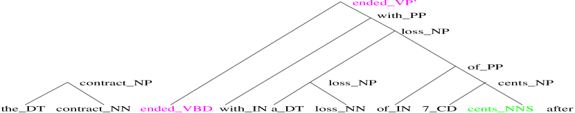
Consider predicting the word after in the sentence:
the contract ended with a loss of 7 cents
after trading as low as 89 cents.
A 3-gram approach would predict after from (7, cents) whereas it is intuitively clear that the strongest predictor would be ended which is outside the reach of even 7-grams. Our assumption is that what enables humans to make a good prediction of after is the syntactic structure in the past. The linguistically correct partial parse of the word history when predicting after is shown in Figure 1. The word ended is called the headword of the constituent (ended (with (...))) and ended is an exposed headword when predicting after — topmost headword in the largest constituent that contains it. The syntactic structure in the past filters out irrelevant words and points to the important ones, thus enabling the use of long distance information when predicting the next word.

Figure 1: Partial parse

Our model will attempt to build the syntactic structure incrementally while traversing the sentence left-to-right. The model will assign a probability $P(W,T)$ to every sentence $W$ with every possible POStag assignment, binary branching parse, non-terminal label and headword annotation for every constituent of $T$.

Let $W$ be a sentence of length $n$ words to which we have prepended <s> and appended </s> so that $w_{0}=$<s> and $w_{n+1}=$</s>. Let $W_{k}$ be the word k-prefix $w_{0}\ldots w_{k}$ of the sentence and $W_{k}T_{k}$ the word-parse k-prefix. To stress this point, a word-parse k-prefix contains — for a given parse — only those binary subtrees whose span is completely included in the word k-prefix, excluding $w_{0}=$<s>. Single words along with their POStag can be regarded as root-only trees. Figure 2 shows a word-parse k-prefix; h_0 .. h_{-m} are the exposed heads, each head being a pair(headword, non-terminal label), or (word, POStag) in the case of a root-only tree.

Figure 2: A word-parse k-prefix

A complete parse — Figure 3 — is any binary parse of the
$(w_{1},t_{1})\ldots(w_{n},t_{n})$ (¡/s¿, SE)+ sequence with the restriction that (</s>, TOP’) is the only allowed head. Note that $((w_{1},t_{1})\ldots(w_{n},t_{n}))$ needn’t be a constituent, but for the parses where it is, there is no restriction on which of its words is the headword or what is the non-terminal label that accompanies the headword.

Figure 3: Complete parse

The model will operate by means of three modules:
$\bullet$ WORD-PREDICTOR predicts the next word $w_{k+1}$ given the word-parse k-prefix and then passes control to the TAGGER;
$\bullet$ TAGGER predicts the POStag of the next word $t_{k+1}$ given the word-parse k-prefix and the newly predicted word and then passes control to the PARSER;
$\bullet$ PARSER grows the already existing binary branching structure by repeatedly generating the transitions:
(unary, NTlabel), (adjoin-left, NTlabel) or (adjoin-right, NTlabel) until it passes control to the PREDICTOR by taking a null transition. NTlabel is the non-terminal label assigned to the newly built constituent and {left,right} specifies where the new headword is inherited from.

The operations performed by the PARSER are illustrated in Figures 4-6 and they ensure that all possible binary branching parses with all possible headword and non-terminal label assignments for the $w_{1}\ldots w_{k}$ word sequence can be generated. The following algorithm formalizes the above description of the sequential generation of a sentence with a complete parse.

Transition t;         // a PARSER transition
predict (<s>, SB);
do{
  //WORD-PREDICTOR and TAGGER
  predict (next_word, POStag);
  //PARSER
  do{
    if(h_{-1}.word != <s>){
      if(h_0.word == </s>)
        t = (adjoin-right, TOP’);
      else{
        if(h_0.tag == NTlabel)
          t = [(adjoin-{left,right}, NTlabel),
               null];
        else
          t = [(unary, NTlabel),
               (adjoin-{left,right}, NTlabel),
               null];
      }
    }
    else{
      if(h_0.tag == NTlabel)
        t = null;
      else
        t = [(unary, NTlabel), null];
    }
  }while(t != null) //done PARSER
}while(!(h_0.word==</s> && h_{-1}.word==<s>))
t = (adjoin-right, TOP); //adjoin <s>_SB; DONE;

Figure 4: Before an adjoin operation

Figure 5: Result of adjoin-left under NTlabel

Figure 6: Result of adjoin-right under NTlabel

The unary transition is allowed only when the most recent exposed head is a leaf of the tree — a regular word along with its POStag — hence it can be taken at most once at a given position in the input word string. The second subtree in Figure 2 provides an example of a unary transition followed by a null transition.

It is easy to see that any given word sequence with a possible parse and headword annotation is generated by a unique sequence of model actions. This will prove very useful in initializing our model parameters from a treebank — see section 3.5.

3 Probabilistic Model

The probability $P(W,T)$ of a word sequence $W$ and a complete parse $T$ can be broken into:

$$P(W,T)=$$ (1)

$$\prod_{k=1}^{n+1}[ P(w_{k}/W_{k-1}T_{k-1})\cdot P(t_{k}/W_{k-1}T_{k-1},w_{k})\cdot$$

$$\prod_{i=1}^{N_{k}}P(p_{i}^{k}/W_{k-1}T_{k-1},w_{k},t_{k},p_{1}^{k}\ldots p_{i-1}^{k})]$$

where:
$\bullet$ $W_{k-1}T_{k-1}$ is the word-parse $(k-1)$-prefix
$\bullet$ $w_{k}$ is the word predicted by WORD-PREDICTOR
$\bullet$ $t_{k}$ is the tag assigned to $w_{k}$ by the TAGGER
$\bullet$ $N_{k}-1$ is the number of operations the PARSER executes before passing control to the WORD-PREDICTOR (the $N_{k}$-th operation at position k is the null transition); $N_{k}$ is a function of $T$
$\bullet$ $p_{i}^{k}$ denotes the i-th PARSER operation carried out at position k in the word string;
$p_{1}^{k}\in\{$(unary, NTlabel)+, (adjoin-left, NTlabel)+,
(adjoin-right, NTlabel), null+$\}$,
$p_{i}^{k}\in\{$ (adjoin-left, NTlabel)+,
(adjoin-right, NTlabel)+$\},1<i<N_{k}$ ,
$p_{i}^{k}=$null+$,i=N_{k}$

Our model is based on three probabilities:

$$P(w_{k}/W_{k-1}T_{k-1})$$ (2)

$$P(t_{k}/w_{k},W_{k-1}T_{k-1})$$ (3)

$$P(p_{i}^{k}/w_{k},t_{k},W_{k-1}T_{k-1},p_{1}^{k}\ldots p_{i-1}^{k})$$ (4)

As can be seen, $(w_{k},t_{k},W_{k-1}T_{k-1},p_{1}^{k}\ldots p_{i-1}^{k})$ is one of the $N_{k}$ word-parse k-prefixes $W_{k}T_{k}$ at position $k$ in the sentence, $i=\overline{1,N_{k}}$.

To ensure a proper probabilistic model (1) we have to make sure that (2), (3) and (4) are well defined conditional probabilities and that the model halts with probability one. Consequently, certain PARSER and WORD-PREDICTOR probabilities must be given specific values:
$\bullet$ $P($null$/W_{k}T_{k})=1$, if h_{-1}.word = <s> and h_{0} $\neq$ (</s>, TOP’) — that is, before predicting </s> — ensures that (<s>, SB) is adjoined in the last step of the parsing process;
$\bullet$ $P($(adjoin-right, TOP)+$/W_{k}T_{k})=1$, if
h_0 = (</s>, TOP’) and h_{-1}.word = <s>
and
$P($(adjoin-right, TOP’)+$/W_{k}T_{k})=1$, if
h_0 = (</s>, TOP’) and h_{-1}.word $\neq$ <s>
ensure that the parse generated by our model is consistent with the definition of a complete parse;
$\bullet$ $P($(unary, NTlabel)$/W_{k}T_{k})=0$, if h_0.tag $\neq$ POStag ensures correct treatment of unary productions;
$\bullet$ $\exists\epsilon>0,\forall W_{k-1}T_{k-1},P(w_{k}$=¡/s¿+$/W_{k-1}T_{k-1})\geq\epsilon$
ensures that the model halts with probability one.

The word-predictor model (2) predicts the next word based on the preceding 2 exposed heads, thus making the following equivalence classification:

$$P(w_{k}/W_{k-1}T_{k-1})=P(w_{k}/h_{0},h_{-1})$$

After experimenting with several equivalence classifications of the word-parse prefix for the tagger model, the conditioning part of model (3) was reduced to using the word to be tagged and the tags of the two most recent exposed heads:

$$P(t_{k}/w_{k},W_{k-1}T_{k-1})=P(t_{k}/w_{k},h_{0}.tag,h_{-1}.tag)$$

Model (4) assigns probability to different parses of the word k-prefix by chaining the elementary operations described above. The workings of the parser module are similar to those of Spatter [Jelinek et al.1994]. The equivalence classification of the $W_{k}T_{k}$ word-parse we used for the parser model (4) was the same as the one used in [Collins1996]:

$$P(p_{i}^{k}/W_{k}T_{k})=P(p_{i}^{k}/h_{0},h_{-1})$$

It is worth noting that if the binary branching structure developed by the parser were always right-branching and we mapped the POStag and non-terminal label vocabularies to a single type then our model would be equivalent to a trigram language model.

3.1 Modeling Tools

All model components — WORD-PREDICTOR, TAGGER, PARSER — are conditional probabilistic models of the type $P(y/x_{1},x_{2},\ldots,x_{n})$ where $y,x_{1},x_{2},\ldots,x_{n}$ belong to a mixed bag of words, POStags, non-terminal labels and parser operations ($y$ only). For simplicity, the modeling method we chose was deleted interpolation among relative frequency estimates of different orders $f_{n}(\cdot)$ using a recursive mixing scheme:

$$P(y/x_{1},\ldots,x_{n})=$$ (5)

$$\lambda(x_{1},\ldots,x_{n})\cdot P(y/x_{1},\ldots,x_{n-1})+$$

$$(1-\lambda(x_{1},\ldots,x_{n}))\cdot f_{n}(y/x_{1},\ldots,x_{n}),$$

$$f_{-1}(y)=uniform(vocabulary(y))$$ (6)

As can be seen, the context mixing scheme discards items in the context in right-to-left order. The $\lambda$ coefficients are tied based on the range of the count $C(x_{1},\ldots,x_{n})$. The approach is a standard one which doesn’t require an extensive description given the literature available on it [Jelinek and Mercer1980].

3.2 Search Strategy

Since the number of parses for a given word prefix $W_{k}$ grows exponentially with $k$, $|\{T_{k}\}|\sim O(2^{k})$, the state space of our model is huge even for relatively short sentences so we had to use a search strategy that prunes it. Our choice was a synchronous multi-stack search algorithm which is very similar to a beam search.

Each stack contains hypotheses — partial parses — that have been constructed by the same number of predictor and the same number of parser operations. The hypotheses in each stack are ranked according to the $\ln(P(W,T))$ score, highest on top. The width of the search is controlled by two parameters:
$\bullet$ the maximum stack depth — the maximum number of hypotheses the stack can contain at any given state;
$\bullet$ log-probability threshold — the difference between the log-probability score of the top-most hypothesis and the bottom-most hypothesis at any given state of the stack cannot be larger than a given threshold.

Figure 7 shows schematically the operations associated with the scanning of a new word $w_{k+1}$.

Figure 7: One search extension cycle

The above pruning strategy proved to be insufficient so we chose to also discard all hypotheses whose score is more than the log-probability threshold below the score of the topmost hypothesis. This additional pruning step is performed after all hypotheses in stage $k^{\prime}$ have been extended with the null parser transition and thus prepared for scanning a new word.

3.3 Word Level Perplexity

The conditional perplexity calculated by assigning to a whole sentence the probability:

$$P(W/T^{*})=\prod_{k=0}^{n}P(w_{k+1}/W_{k}T_{k}^{*}),$$ (7)

where $T^{*}=argmax_{T}P(W,T)$, is not valid because it is not causal: when predicting $w_{k+1}$ we use $T^{*}$ which was determined by looking at the entire sentence. To be able to compare the perplexity of our model with that resulting from the standard trigram approach, we need to factor in the entropy of guessing the correct parse $T_{k}^{*}$ before predicting $w_{k+1}$, based solely on the word prefix $W_{k}$.

The probability assignment for the word at position $k+1$ in the input sentence is made using:

$$P(w_{k+1}/W_{k})=$$ (8)

$$\sum_{T_{k}\in S_{k}}P(w_{k+1}/W_{k}T_{k})\cdot\rho(W_{k},T_{k}),$$

$$\rho(W_{k},T_{k})=P(W_{k}T_{k})/\sum_{T_{k}\in S_{k}}P(W_{k}T_{k})$$ (9)

which ensures a proper probability over strings $W^{*}$, where $S_{k}$ is the set of all parses present in our stacks at the current stage $k$.

Another possibility for evaluating the word level perplexity of our model is to approximate the probability of a whole sentence:

$$P(W)=\sum_{k=1}^{N}P(W,T^{(k)})$$ (10)

where $T^{(k)}$ is one of the “N-best” — in the sense defined by our search — parses for $W$. This is a deficient probability assignment, however useful for justifying the model parameter re-estimation.

The two estimates (8) and (10) are both consistent in the sense that if the sums are carried over all possible parses we get the correct value for the word level perplexity of our model.

3.4 Parameter Re-estimation

The major problem we face when trying to reestimate the model parameters is the huge state space of the model and the fact that dynamic programming techniques similar to those used in HMM parameter re-estimation cannot be used with our model. Our solution is inspired by an HMM re-estimation technique that works on pruned — N-best — trellises[Byrne et al.1998].

Let $(W,T^{(k)}),k=1\ldots N$ be the set of hypotheses that survived our pruning strategy until the end of the parsing process for sentence $W$. Each of them was produced by a sequence of model actions, chained together as described in section 2; let us call the sequence of model actions that produced a given $(W,T)$ the $derivation(W,T)$.

Let an elementary event in the $derivation(W,T)$ be $(y_{l}^{(m_{l})},{\underline{x}}_{l}^{(m_{l})})$ where:
$\bullet$ $l$ is the index of the current model action;
$\bullet$ $m_{l}$ is the model component — WORD-PREDICTOR, TAGGER, PARSER — that takes action number $l$ in the $derivation(W,T)$;
$\bullet$ $y_{l}^{(m_{l})}$ is the action taken at position $l$ in the derivation:
if $m_{l}$ = WORD-PREDICTOR, then $y_{l}^{(m_{l})}$ is a word;
if $m_{l}$ = TAGGER, then $y_{l}^{(m_{l})}$ is a POStag;
if $m_{l}$ = PARSER, then $y_{l}^{(m_{l})}$ is a parser-action;
$\bullet$ ${\underline{x}}_{l}^{(m_{l})}$ is the context in which the above action was taken:
if $m_{l}$ = WORD-PREDICTOR or PARSER, then ${\underline{x}}_{l}^{(m_{l})}=(h_{0}.tag,h_{0}.word,h_{-1}.tag,h_{-1}.word)$;
if $m_{l}$ = TAGGER, then
${\underline{x}}_{l}^{(m_{l})}=($word-to-tag$,h_{0}.tag,h_{-1}.tag)$.

The probability associated with each model action is determined as described in section 3.1, based on counts $C^{(m)}(y^{(m)},{\underline{x}}^{(m)})$, one set for each model component.

Assuming that the deleted interpolation coefficients and the count ranges used for tying them stay fixed, these counts are the only parameters to be re-estimated in an eventual re-estimation procedure; indeed, once a set of counts $C^{(m)}(y^{(m)},{\underline{x}}^{(m)})$ is specified for a given model $m$, we can easily calculate:
$\bullet$ the relative frequency estimates
$f_{n}^{(m)}(y^{(m)}/{\underline{x}}_{n}^{(m)})$ for all context orders $n=0\ldots$maximum-order$(model(m))$;
$\bullet$ the count $C^{(m)}({\underline{x}}_{n}^{(m)})$ used for determining the $\lambda({\underline{x}}_{n}^{(m)})$ value to be used with the order-$n$ context ${\underline{x}}_{n}^{(m)}$.
This is all we need for calculating the probability of an elementary event and then the probability of an entire derivation.

One training iteration of the re-estimation procedure we propose is described by the following algorithm:

N-best parse development data; // counts.Ei
// prepare counts.E(i+1)
for each model component c{
  gather_counts development model_c;
}

In the parsing stage we retain for each “N-best” hypothesis $(W,T^{(k)}),k=1\ldots N,$ only the quantity
$\phi(W,T^{(k)})=P(W,T^{(k)})/\sum_{k=1}^{N}P(W,T^{(k)})$
and its $derivation(W,T^{(k)})$. We then scan all the derivations in the “development set” and, for each occurrence of the elementary event $(y^{(m)},{\underline{x}}^{(m)})$ in $derivation(W,T^{(k)})$ we accumulate the value $\phi(W,T^{(k)})$ in the $C^{(m)}(y^{(m)},{\underline{x}}^{(m)})$ counter to be used in the next iteration.

The intuition behind this procedure is that $\phi(W,T^{(k)})$ is an approximation to the $P(T^{(k)}/W)$ probability which places all its mass on the parses that survived the parsing process; the above procedure simply accumulates the expected values of the counts $C^{(m)}(y^{(m)},{\underline{x}}^{(m)})$ under the $\phi(W,T^{(k)})$ conditional distribution. As explained previously, the $C^{(m)}(y^{(m)},{\underline{x}}^{(m)})$ counts are the parameters defining our model, making our procedure similar to a rigorous EM approach [Dempster et al.1977].

A particular — and very interesting — case is that of events which had count zero but get a non-zero count in the next iteration, caused by the “N-best” nature of the re-estimation process. Consider a given sentence in our “development” set. The “N-best” derivations for this sentence are trajectories through the state space of our model. They will change from one iteration to the other due to the smoothing involved in the probability estimation and the change of the parameters — event counts — defining our model, thus allowing new events to appear and discarding others through purging low probability events from the stacks. The higher the number of trajectories per sentence, the more dynamic this change is expected to be.

The results we obtained are presented in the experiments section. All the perplexity evaluations were done using the left-to-right formula (8) (L2R-PPL) for which the perplexity on the “development set” is not guaranteed to decrease from one iteration to another. However, we believe that our re-estimation method should not increase the approximation to perplexity based on (10) (SUM-PPL) — again, on the “development set”; we rely on the consistency property outlined at the end of section 3.3 to correlate the desired decrease in L2R-PPL with that in SUM-PPL. No claim can be made about the change in either L2R-PPL or SUM-PPL on test data.

3.5 Initial Parameters

Each model component — WORD-PREDICTOR, TAGGER, PARSER — is trained initially from a set of parsed sentences, after each parse tree $(W,T)$ undergoes:
$\bullet$ headword percolation and binarization — see section 4;
$\bullet$ decomposition into its $derivation(W,T)$.
Then, separately for each $m$ model component, we:
$\bullet$ gather joint counts $C^{(m)}(y^{(m)},{\underline{x}}^{(m)})$ from the derivations that make up the “development data” using $\phi(W,T)=1$;
$\bullet$ estimate the deleted interpolation coefficients on joint counts gathered from “check data” using the EM algorithm.
These are the initial parameters used with the re-estimation procedure described in the previous section.

4 Headword Percolation and Binarization

In order to get initial statistics for our model components we needed to binarize the UPenn Treebank [Marcus et al.1995] parse trees and percolate headwords. The procedure we used was to first percolate headwords using a context-free (CF) rule-based approach and then binarize the parses by using a rule-based approach again.

The headword of a phrase is the word that best represents the phrase, all the other words in the phrase being modifiers of the headword. Statistically speaking, we were satisfied with the output of an enhanced version of the procedure described in [Collins1996] — also known under the name “Magerman & Black Headword Percolation Rules”.

Once the position of the headword within a constituent — equivalent with a CF production of the type $Z\rightarrow Y_{1}\ldots Y_{n}$ , where $Z,Y_{1},\ldots Y_{n}$ are non-terminal labels or POStags (only for $Y_{i}$) — is identified to be $k$, we binarize the constituent as follows: depending on the $Z$ identity, a fixed rule is used to decide which of the two binarization schemes in Figure 8 to apply. The intermediate nodes created by the above binarization schemes receive the non-terminal label $Z^{\prime}$.

Figure 8: Binarization schemes

5 Experiments

Due to the low speed of the parser — 200 wds/min for stack depth 10 and log-probability threshold 6.91 nats (1/1000) — we could carry out the re-estimation technique described in section 3.4 on only 1 Mwds of training data. For convenience we chose to work on the UPenn Treebank corpus. The vocabulary sizes were:
$\bullet$ word vocabulary: 10k, open — all words outside the vocabulary are mapped to the <unk> token;
$\bullet$ POS tag vocabulary: 40, closed;
$\bullet$ non-terminal tag vocabulary: 52, closed;
$\bullet$ parser operation vocabulary: 107, closed;
The training data was split into “development” set — 929,564wds (sections 00-20) — and “check set” — 73,760wds (sections 21-22); the test set size was 82,430wds (sections 23-24). The “check” set has been used for estimating the interpolation weights and tuning the search parameters; the “development” set has been used for gathering/estimating counts; the test set has been used strictly for evaluating model performance.

Table 1 shows the results of the re-estimation technique presented in section 3.4. We achieved a reduction in test-data perplexity bringing an improvement over a deleted interpolation trigram model whose perplexity was 167.14 on the same training-test data; the reduction is statistically significant according to a sign test.

iteration	DEV set	TEST set
number	L2R-PPL	L2R-PPL
E0	24.70	167.47
E1	22.34	160.76
E2	21.69	158.97
E3	21.26	158.28
3-gram	21.20	167.14

Table 1: Parameter re-estimation results

Simple linear interpolation between our model and the trigram model:

$$Q(w_{k+1}/W_{k})=$$

$$\lambda\cdot P(w_{k+1}/w_{k-1},w_{k})+(1-\lambda)\cdot P(w_{k+1}/W_{k})$$

yielded a further improvement in PPL, as shown in Table 2. The interpolation weight was estimated on check data to be $\lambda=0.36$.

iteration	TEST set	TEST set
number	L2R-PPL	3-gram interpolated PPL
E0	167.47	152.25
E3	158.28	148.90
3-gram	167.14	167.14

Table 2: Interpolation with trigram results

An overall relative reduction of 11% over the trigram model has been achieved.

6 Conclusions and Future Directions

The large difference between the perplexity of our model calculated on the “development” set — used for model parameter estimation — and “test” set — unseen data — shows that the initial point we choose for the parameter values has already captured a lot of information from the training data. The same problem is encountered in standard n-gram language modeling; however, our approach has more flexibility in dealing with it due to the possibility of reestimating the model parameters.

We believe that the above experiments show the potential of our approach for improved language models. Our future plans include:
$\bullet$ experiment with other parameterizations than the two most recent exposed heads in the word predictor model and parser;
$\bullet$ estimate a separate word predictor for left-to-right language modeling. Note that the corresponding model predictor was obtained via re-estimation aimed at increasing the probability of the ”N-best” parses of the entire sentence;
$\bullet$ reduce vocabulary of parser operations; extreme case: no non-terminal labels/POS tags, word only model; this will increase the speed of the parser thus rendering it usable on larger amounts of training data and allowing the use of deeper stacks — resulting in more “N-best” derivations per sentence during re-estimation;
$\bullet$ relax — flatten — the initial statistics in the re-estimation of model parameters; this would allow the model parameters to converge to a different point that might yield a lower word-level perplexity;
$\bullet$ evaluate model performance on n-best sentences output by an automatic speech recognizer.

7 Acknowledgments

This research has been funded by the NSF
IRI-19618874 grant (STIMULATE).

The authors would like to thank to Sanjeev Khudanpur for his insightful suggestions. Also to Harry Printz, Eric Ristad, Andreas Stolcke, Dekai Wu and all the other members of the dependency modeling group at the summer96 DoD Workshop for useful comments on the model, programming support and an extremely creative environment. Also thanks to Eric Brill, Sanjeev Khudanpur, David Yarowsky, Radu Florian, Lidia Mangu and Jun Wu for useful input during the meetings of the people working on our STIMULATE grant.

References

- [\citenameByrne et al.1998] W. Byrne, A. Gunawardana, and S. Khudanpur. 1998. Information geometry and EM variants. Technical Report CLSP Research Note 17, Department of Electical and Computer Engineering, The Johns Hopkins University, Baltimore, MD.
- [\citenameChelba et al.1997] C. Chelba, D. Engle, F. Jelinek, V. Jimenez, S. Khudanpur, L. Mangu, H. Printz, E. S. Ristad, R. Rosenfeld, A. Stolcke, and D. Wu. 1997. Structure and performance of a dependency language model. In Proceedings of Eurospeech, volume 5, pages 2775–2778. Rhodes, Greece.
- [\citenameCollins1996] Michael John Collins. 1996. A new statistical parser based on bigram lexical dependencies. In Proceedings of the 34th Annual Meeting of the Association for Computational Linguistics, pages 184–191. Santa Cruz, CA.
- [\citenameDempster et al.1977] A. P. Dempster, N. M. Laird, and D. B. Rubin. 1977. Maximum likelihood from incomplete data via the EM algorithm. In Journal of the Royal Statistical Society, volume 39 of B, pages 1–38.
- [\citenameJelinek and Mercer1980] Frederick Jelinek and Robert Mercer. 1980. Interpolated estimation of markov source parameters from sparse data. In E. Gelsema and L. Kanal, editors, Pattern Recognition in Practice, pages 381–397.
- [\citenameJelinek et al.1994] F. Jelinek, J. Lafferty, D. M. Magerman, R. Mercer, A. Ratnaparkhi, and S. Roukos. 1994. Decision tree parsing using a hidden derivational model. In ARPA, editor, Proceedings of the Human Language Technology Workshop, pages 272–277.
- [\citenameMarcus et al.1995] M. Marcus, B. Santorini, and M. Marcinkiewicz. 1995. Building a large annotated corpus of English: the Penn Treebank. Computational Linguistics, 19(2):313–330.
- [\citenamePhilips1996] Colin Philips. 1996. Order and Structure. Ph.D. thesis, MIT. Distributed by MITWPL.