Equivalence Is In The Eye Of The Beholder

Abstract

In a recent provocative paper, Lamport points out ”the insubstantiality of processes” by proving the equivalence of two different decompositions of the same intuitive algorithm by means of temporal formulas. We point out that the correct equivalence of algorithms is itself in the eye of the beholder. We discuss a number of related issues and, in particular, whether algorithms can be proved equivalent directly.

1 Introduction

This is a reaction to Leslie Lamport’s “Processes are in the Eye of the Beholder” [13]. Lamport writes:

A concurrent algorithm is traditionally represented as the composition of processes. We show by an example that processes are an artifact of how an algorithm is represented. The difference between a two-process representation and a four-process representation of the same algorithm is no more fundamental than the difference between $2+2$ and $1+1+1+1$.

To demonstrate his thesis, Lamport uses two different programs for a first-in, first-out ring buffer of size $N$. He represents the two algorithms by temporal formulas and proves the equivalence of the two temporal formulas.

We analyze in what sense the two algorithms are and are not equivalent. There is no one notion of equivalence appropriate for all purposes and thus the “insubstantiality of processes” may itself be in the eye of the beholder. There are other issues where we disagree with Lamport. In particular, we give a direct equivalence proof for two programs without representing them by means of temporal formulas.

This paper is self-contained. In the remainder of this section, we explain the two ring buffer algorithms and discuss our disagreements with Lamport. In Section 2, we give a brief introduction to evolving algebras. In Section 3, we present our formalizations of the ring buffer algorithms as evolving algebras. In Section 4, we define a version of lock-step equivalence and prove that our formalizations of these algorithms are equivalent in that sense. Finally, we discuss the inequivalence of these algorithms in Section 5.

1.1 Ring Buffer Algorithms

The ring buffer in question is implemented by means of an array of $N$ elements. The $i$th input (starting with $i=0$) is stored in slot $i\bmod N$ until it is sent out as the $i$th output. Items may be placed in the buffer if and only if the buffer is not full; of course, items may be sent from the buffer if and only if the buffer is not empty. Input number $i$ cannot occur until (1) all previous inputs have occurred and (2) either $i<N$ or else output number $i-N$ has occurred. Output number $i$ cannot occur until (1) all previous outputs have occurred and (2) input number $i$ has occurred. These dependencies are illustrated pictorially in Figure 1, where circles represent the actions to be taken and arrows represent dependency relationships between actions.

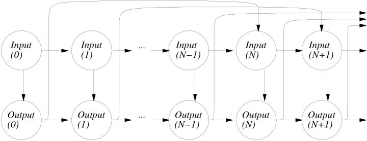
Figure 1: Moves of the ring-buffer algorithm.

Lamport writes the two programs in a semi-formal language reminiscent of CSP [9] which we call Pseudo-CSP. The first program, which we denote by ${\cal R}_{\mathrm{pcsp}}$, is shown in Figure 2. It operates the buffer using two processes; one handles input into the buffer and the other handles output from the buffer. It gives rise to a row-wise decomposition of the graph of moves, as shown in Figure 3. The second program, which we denote by ${\cal C}_{\mathrm{pcsp}}$, is shown in Figure 4. It uses $N$ processes, each managing input and output for one particular slot in the buffer. It gives rise to a column-wise decomposition of the graph of moves, as shown in Figure 5.

$\begin{array}[]{l}\mbox{\em in,\ out}:\mbox{\bf channel\ of\ }\mbox{\em Value}\\ \mbox{\em buf}:\mbox{\bf array\ }0\ldots N-1\mbox{\bf\ of\ }\mbox{\em Value}\\ p,g:\mbox{\bf internal\ }\mbox{\em Natural\ }\mbox{\bf initially\ }0\\ \begin{array}[]{ll}\mbox{\em Receiver}::&*\left[\begin{array}[]{rcl}p-g\neq N&\rightarrow&\mbox{\em in\ }?\mbox{\em buf\ }[p\bmod N];\\ &&p:=p+1\end{array}\right]\\ \quad\|\\ \mbox{\em Sender}::&*\left[\begin{array}[]{rcl}p-g\neq 0&\rightarrow&\mbox{\em out\ }!\mbox{\em buf\ }[g\bmod N];\\ &&g:=g+1\end{array}\right]\end{array}\end{array}$

Figure 2: A two-process ring buffer ${\cal R}_{\mathrm{pcsp}}$, in Pseudo-CSP.

Figure 3: Moves of ${\cal R}_{\mathrm{pcsp}}$.

$\begin{array}[]{l}\mbox{\em in,\ out}:\mbox{\bf channel\ of\ }\mbox{\em Value}\\ \mbox{\em buf}:\mbox{\bf array\ }0\ldots N-1\mbox{\ of\ }\mbox{\em Value}\\ pp,gg:\mbox{\bf internal\ array\ }0\ldots N-1\mbox{\bf\ of\ }\{0,1\}\mbox{\bf\ initially\ }0\\ \mbox{\em Buffer}(i:0\ldots N-1)::\\ \quad*\left[\begin{array}[]{rcl}\mbox{\em empty}:\ \mbox{\em IsNext}(pp,i)&\rightarrow&\mbox{\em in\ }?\mbox{\em buf\ }[i];\\ &&pp[i]:=(pp[i]+1)\bmod 2;\\ \mbox{\em full}:\ \mbox{\em IsNext}(gg,i)&\rightarrow&\mbox{\em out\ }!\mbox{\em buf\ }[i];\\ &&gg[i]:=(gg[i]+1)\bmod 2;\end{array}\right]\\ \\ \begin{array}[]{rllll}\mbox{\em IsNext}(r,i)&\stackrel{{\scriptstyle\triangle}}{{=}}&\mbox{\bf if\ }\ i=0&\mbox{\bf\ then\ }&r[0]=r[N-1]\\ &&&\mbox{\bf\ else\ }&r[i]\neq r[i-1]\end{array}\end{array}$

Figure 4: An $N$ process ring buffer ${\cal C}_{\mathrm{pcsp}}$, in Pseudo-CSP.

Figure 5: Moves of ${\cal C}_{\mathrm{pcsp}}$.

In Pseudo-CSP, the semicolon represents sequential composition, $\|$ represents parallel composition, and $*$ represents iteration. The general meanings of ? and ! are more complicated; they indicate synchronization. In the context of ${\cal R}_{\mathrm{pcsp}}$ and ${\cal C}_{\mathrm{pcsp}}$, “in ?” is essentially a command to place the current input into the given slot, and “out !” is essentially a command to send out the datum in the given slot as an output. In Section 3, we will give a more complete explanation of the two programs in terms of evolving algebras.

After presenting the two algorithms in Pseudo-CSP, Lamport describes them by means of formulas in TLA, the Temporal Logic of Actions [12], and proves the equivalence of the two formulas in TLA. He does not prove that the TLA formulas are equivalent to the corresponding Pseudo-CSP programs. The Pseudo-CSP presentations are there only to guide the reader’s intuition. As we have mentioned, Pseudo-CSP is only semi-formal; neither the syntax nor the semantics of it is given precisely.

However, Lamport provides a hint as to why the two programs themselves are equivalent. There is a close correspondence of values between $p$ and $pp$, and between $g$ and $gg$. Figure 6, taken from [13], illustrates the correspondence between $p$ and $pp$ for $N=4$. The $n$th row describes the values of variables $p$ and $pp$ after $n$ inputs. The predicate IsNext(pp,i) is intended to be true only for one array position $i$ at any state (the position that is going to be active); the box indicates that position.

$\begin{array}[]{cccccc}p&&pp[0]&pp[1]&pp[2]&pp[3]\\ \\ 0&&\framebox{0}&0&0&0\\ 1&&1&\framebox{0}&0&0\\ 2&&1&1&\framebox{0}&0\\ 3&&1&1&1&\framebox{0}\\ 4&&\framebox{1}&1&1&1\\ 5&&0&\framebox{1}&1&1\\ 6&&0&0&\framebox{1}&1\\ \vdots&&\vdots&\vdots&\vdots&\vdots\\ \end{array}$

Figure 6: The correspondence between values of $pp$ and $p$, for $N=4$.

1.2 Discussion

There are three issues where we disagree with Lamport.

Issue 1: The Notion of Equivalence.

What does it mean that two programs are equivalent? In our opinion, the answer to the question depends on the desired abstraction [4]. There are many reasonable definitions of equivalence. Here are some examples.

1. The two programs produce the same output on the same input.

2. The two programs produce the same output on the same input, and the two programs are of the same time complexity (with respect to your favorite definition of time complexity).

3. Given the same input, the two programs produce the same output and take precisely the same amount of time.

4. No observer of the execution of the two programs can detect any difference.

The reader will be able to suggest numerous other reasonable definitions for equivalence. For example, one could substitute space for time in conditions (2) and (3) above. The nature of an “observer” in condition (4) admits different plausible interpretations, depending upon what aspects of the execution the observer is allowed to observe.

Let us stress that we do not promote any particular notion of equivalence or any particular class of such notions. We only note that there are different reasonable notions of equivalence and there is no one notion of equivalence that is best for all purposes. The two ring-buffer programs are indeed “strongly equivalent”; in particular, they are equivalent in the sense of definition (3) above. However, they are not equivalent in the sense of definition (4) for certain observers, or in the sense of some space-complexity versions of definitions (2) and (3). See Section 5 in this connection.

Issue 2: Representing Programs as Formulas.

Again, we quote Lamport [13]:

We will not attempt to give a rigorous meaning to the program text. Programming languages evolved as a method of describing algorithms to compilers, not as a method for reasoning about them. We do not know how to write a completely formal proof that two programming language representations of the ring buffer are equivalent. In Section 2, we represent the program formally in TLA, the Temporal Logic of Actions [12].

We believe that it is not only possible but also beneficial to give a rigorous meaning to one’s programming language and to prove the desired equivalence of programs directly. The evolving algebra method has been used to give rigorous meaning to various programming languages [1, 10]. In a similar way, one may try to give formal semantics to Pseudo-CSP (which is used in fact for describing algorithms to humans, not compilers). Taking into account the modesty of our goals in this paper, we do not do that and represent ${\cal R}_{\mathrm{pcsp}}$ and ${\cal C}_{\mathrm{pcsp}}$ directly as evolving algebra programs ${\cal R}_{\mathrm{ea}}$ and ${\cal C}_{\mathrm{ea}}$ and then work with the two evolving algebras.

One may argue that our translation is not perfectly faithful. Of course, no translation from a semi-formal to a formal language can be proved to be faithful. We believe that our translation is reasonably faithful; we certainly did not worry about the complexity of our proofs as we did our translations. Also, we do not think that Lamport’s TLA description of the Pseudo-CSP is perfectly faithful (see the discussion in subsection 3.2) and thus we have two slightly different ideals to which we can be faithful. In fact, we do not think that perfect faithfulness is crucially important here. We give two programming language representations ${\cal R}_{\mathrm{ea}}$ and ${\cal C}_{\mathrm{ea}}$ of the ring buffer reflecting different decompositions of the buffer into processes. Confirming Lamport’s thesis, we prove that the two programs are equivalent in a very strong sense; our equivalence proof is direct. Then we point out that our programs are inequivalent according to some natural definitions of equivalence. Moreover, the same inequivalence arguments apply to ${\cal R}_{\mathrm{pcsp}}$ and ${\cal C}_{\mathrm{pcsp}}$ as well.

Issue 3: The Formality of Proofs.

Continuing, Lamport writes [13]:

We now give a hierarchically structured proof that $\Pi_{2}$ and $\Pi_{N}$ [the TLA translations of ${\cal R}_{\mathrm{pcsp}}$ and ${\cal C}_{\mathrm{pcsp}}$ – GH] are equivalent [11]. The proof is completely formal, meaning that each step is a mathematical formula. English is used only to explain the low-level reasoning. The entire proof could be carried down to a level at which each step follows from the simple application of formal rules, but such a detailed proof is more suitable for machine checking than human reading. Our complete proof, with “Q.E.D.” steps and low-level reasoning omitted, appears in Appendix A.

We prefer to separate the process of explaining a proof to people from the process of computer-aided verification of the same proof [7]. A human-oriented exposition is much easier for humans to read and understand than expositions attempting to satisfy both concerns at once. Writing a good human-oriented proof is the art of creating the correct images in the mind of the reader. Such a proof is amenable to the traditional social process of debugging mathematical proofs.

Granted, mathematicians make mistakes and computer-aided verification may be desirable, especially in safety-critical applications. In this connection we note that a human-oriented proof can be a starting point for mechanical verification. Let us stress also that a human-oriented proof need not be less precise than a machine-oriented proof; it simply addresses a different audience.

Revisiting Lamport’s Thesis

These disagreements do not mean that our position on “the insubstantiality of processes” is the direct opposite of Lamport’s. We simply point out that “the insubstantiality of processes” may itself be in the eye of the beholder. The same two programs can be equivalent with respect to some reasonable definitions of equivalence and inequivalent with respect to others.

2 Evolving Algebras

Evolving algebras were introduced in [5]; a more detailed definition has appeared in [6]. Since its introduction, this methodology has been used for a wide variety of applications: programming language semantics, hardware specification, protocol verification, etc.. It has been used to show equivalences of various kinds, including equivalences across a variety of abstraction levels for various real-world systems, e.g. [3]. See [1, 10] for numerous other examples.

We recall here only as much of evolving algebra definitions [6] as needed in this paper. Evolving algebras (often abbreviated ealgebras or EA) have many other capabilities not shown here: for example, creating or destroying agents during the evolution.

Those already familiar with ealgebras may wish to skip this section.

2.1 States

States are essentially logicians’ structures except that relations are treated as special functions. They are also called static algebras and indeed they are algebras in the sense of the science of universal algebra.

A vocabulary is a finite collection of function names, each of fixed arity. Every vocabulary contains the following logic symbols: nullary function names true, false, undef, the equality sign, (the names of) the usual Boolean operations and (for convenience) a unary function name Bool. Some function symbols are tagged as relation symbols (or predicates); for example, Bool and the equality sign are predicates.

A state $S$ of vocabulary $\Upsilon$ is a non-empty set $X$ (the basic set or superuniverse of $S$), together with interpretations of all function symbols in $\Upsilon$ over $X$ (the basic functions of $S$). A function symbol $f$ of arity $r$ is interpreted as an $r$-ary operation over $X$ (if $r=0$, it is interpreted as an element of $X$). The interpretations of predicates (the basic relations) and the logic symbols satisfy the following obvious requirements. The elements (more exactly, the interpretations of) true and false are distinct. These two elements are the only possible values of any basic relation and the only arguments where Bool produces true. They are operated upon in the usual way by the Boolean operations. The interpretation of undef is distinct from those of true and false. The equality sign is interpreted as the equality relation. We denote the value of a term $t$ in state $S$ by $t_{S}$.

Domains. Let $f$ be a basic function of arity $r$ and $\bar{x}$ range over $r$-tuples of elements of $S$. If $f$ is a basic relation then the domain of $f$ at $S$ is $\{\bar{x}:f(\bar{x})=\mbox{true}\}$. Otherwise the domain of $f$ at $S$ is $\{\bar{x}:f(\bar{x})\neq\mbox{undef}\}$.

Universes. A basic relation $f$ may be viewed as the set of tuples where it evaluates to true. If $f$ is unary it can be viewed as a universe. For example, Bool is a universe consisting of two elements (named) true and false. Universes allow us to view states as many-sorted structures.

Types. Let $f$ be a basic function of arity $r$ and $U_{0},\ldots,U_{r}$ be universes. We say that $f$ is of type $U_{1}\times\cdots\times U_{r}\rightarrow U_{0}$ in the given state if the domain of $f$ is $U_{1}\times\cdots\times U_{r}$ and $f(\bar{x})\in U_{0}$ for every $\bar{x}$ in the domain of $f$. In particular, a nullary $f$ is of type $U_{0}$ if (the value of) $f$ belongs to $U_{0}$.

Example. Consider a directed ring of nodes with two tokens; each node may be colored or uncolored. We formalize this as a state as follows. The superuniverse contains a non-empty universe Nodes comprising the nodes of the ring. Also present is the obligatory two-element universe Bool, disjoint from Nodes. Finally, there is an element (interpreting) undef outside of Bool and outside of Nodes. There is nothing else in the superuniverse. (Usually we skip the descriptions of Bool and undef). A unary function Next indicates the successor to a given node in the ring. Nullary functions Token1 and Token2 give the positions of the two tokens. A unary predicate Colored indicates whether the given node is colored.

2.2 Updates

There is a way to view states which is unusual to logicians. View a state as a sort of memory. Define a location of a state $S$ to be a pair $\ell=(f,\bar{x})$, where $f$ is a function name in the vocabulary of $S$ and $\bar{x}$ is a tuple of elements of (the superuniverse of) $S$ whose length equals the arity of $f$. (If $f$ is nullary, $\ell$ is simply $f$.) In the two-token ring example, let $a$ be any node (that is, any element of the universe Nodes). Then the pair (Next,$a$) is a location.

An update of a state $S$ is a pair $\alpha=(\ell,y)$, where $\ell$ is a location of $S$ and $y$ is an element of $S$. To fire $\alpha$ at $S$, put $y$ into the location $\ell$; that is, if $\ell=(f,\bar{x})$, redefine $S$ to interpret $f(\bar{x})$ as $y$; nothing else (including the superuniverse) is changed. We say that an update $(\ell,y)$ of state $S$ is trivial if $y$ is the content of $\ell$ in $S$. In the two-token ring example, let $a$ be any node. Then the pair (Token1, $a$) is an update. To fire this update, move the first token to the position $a$.

Remark to a curious reader. If $\ell$ = (Next,$a$), then ($\ell,a$) is also an update. To fire this update, redefine the successor of $a$; the new successor is $a$ itself. This update destroys the ring (unless the ring had only one node). To guard from such undesirable changes, the function Next can be declared static (see [6]) which will make any update of Next illegal.

An update set over a state $S$ is a set of updates of $S$. An update set is consistent at $S$ if no two updates in the set have the same location but different values. To fire a consistent set at $S$, fire all its members simultaneously; to fire an inconsistent set at $S$, do nothing. In the two-token ring example, let $a,b$ be two nodes. Then the update set $\{(Token1,a),(Token1,b)\}$ is consistent if and only if $a=b$.

2.3 Basic Transition Rules

We introduce rules for changing states. The semantics for each rule should be obvious. At a given state $S$ whose vocabulary includes that of a rule $R$, $R$ gives rise to an update set $\mbox{US}(R,S)$; to execute $R$ at $S$, one fires $\mbox{US}(R,S)$. We say that $R$ is enabled at $S$ if $\mbox{US}(R,S)$ is consistent and contains a non-trivial update. We suppose below that a state of discourse $S$ has a sufficiently rich vocabulary.

An update instruction $R$ has the form

$f(t_{1},\ldots,t_{r}):=t_{0}$

where $f$ is a function name of arity $r$ and each $t_{i}$ is a term. (If $r=0$ we write “$f:=t_{0}$” rather than “$f():=t_{0}$”.) The update set $\mbox{US}(R,S)$ contains a single element $(\ell,y)$, where $y$ is the value $(t_{0})_{S}$ of $t_{0}$ at $S$ and $\ell=(f,(x_{1},\ldots,x_{r}))$ with $x_{i}=(t_{i})_{S}$. In other words, to execute $R$ at $S$, set $f((t_{1})_{S},\ldots,(t_{r})_{S})$ to $(t_{0})_{S}$ and leave the rest of the state unchanged. In the two-token ring example, “Token1 := Next(Token2)” is an update instruction. To execute it, move token 1 to the successor of (the current position of) token 2.

A block rule $R$ is a sequence $R_{1},\ldots,R_{n}$ of transition rules. To execute $R$ at $S$, execute all the constituent rules at $S$ simultaneously. More formally, $\mbox{US}(R,S)=\bigcup_{i=1}^{n}\mbox{US}(R_{i},S)$. (One is supposed to write “block” and “endblock” to denote the scope of a block rule; we often omit them for brevity.) In the two-token ring example, consider the following block rule:

Token1 := Token2

Token2 := Token1

To execute this rule, exchange the tokens. The new position of Token1 is the old position of Token2, and the new position of Token2 is the old position of Token1.

A conditional rule $R$ has the form

if $g$ then $R_{0}$ endif

where $g$ (the guard) is a term and $R_{0}$ is a rule. If $g$ holds (that is, has the same value as true) in $S$ then $\mbox{US}(R,S)=\mbox{US}(R_{0},S)$; otherwise $\mbox{US}(R,S)=\emptyset$. (A more general form is “if $g$ then $R_{0}$ else $R_{1}$ endif”, but we do not use it in this paper.) In the two-token ring example, consider the following conditional rule:

if Token1 = Token2 then
	Colored(Token1) := true
endif

Its meaning is the following: if the two tokens are at the same node, then color that node.

2.4 Rules with Variables

Basic rules are sufficient for many purposes, e.g. to give operational semantics for the C programming language [8], but in this paper we need two additional rule constructors. The new rules use variables. Formal treatment of variables requires some care but the semantics of the new rules is quite obvious, especially because we do not need to nest constructors with variables here. Thus we skip the formalities and refer the reader to [6]. As above $S$ is a state of sufficiently rich vocabulary.

A parallel synchronous rule (or declaration rule, as in [6]) $R$ has the form:

var $x$ ranges over $U$
	$R(x)$
endvar

where $x$ is a variable name, $U$ is a universe name, and $R(x)$ can be viewed as a rule template with free variable $x$. To execute $R$ at $S$, execute simultaneously all rules $R(u)$ where $u$ ranges over $U$. In the two-token ring example, (the execution of) the following rule colors all nodes except for the nodes occupied by the tokens.

var $x$ ranges over Nodes
	if $x\neq$ Token1 and $x\neq$ Token2 then
		Colored(x) := true
	endif
endvar

A choice rule $R$ has the form

choose $x$ in $U$
	$R(x)$
endchoose

where $x$, $U$ and $R(x)$ are as above. It is nondeterministic. To execute the choice rule, choose arbitrarily one element $u$ in $U$ and execute the rule $R(u)$. In the two-token ring example, each execution of the following rule either colors an unoccupied node or does nothing.

choose $x$ in Nodes
	if $x\neq$ Token1 and $x\neq$ Token2 then
		Colored(x) := true
	endif
endchoose

2.5 Distributed Evolving Algebra Programs

Let $\Upsilon$ be a vocabulary that contains the universe Agents, the unary function Mod and the nullary function Me. A distributed EA program $\Pi$ of vocabulary $\Upsilon$ consists of a finite set of modules, each of which is a transition rule with function names from $\Upsilon$. Each module is assigned a different name; these names are nullary function names from $\Upsilon$ different from Me. Intuitively, a module is the program to be executed by one or more agents.

A (global) state of $\Pi$ is a structure $S$ of vocabulary $\Upsilon$–{Me} where different module names are interpreted as different elements of $S$ and the function Mod assigns (the interpretations of) module names to elements of Agents; Mod is undefined (that is, produces undef) otherwise. If Mod maps an element $\alpha$ to a module name $M$, we say that $\alpha$ is an agent with program $M$.

For each agent $\alpha$, View${}_{\alpha}(S)$ is the reduct of $S$ to the collection of functions mentioned in the module Mod($\alpha$), expanded by interpreting Me as $\alpha$. Think about View${}_{\alpha}(S)$ as the local state of agent $\alpha$ corresponding to the global state $S$. We say that an agent $\alpha$ is enabled at $S$ if Mod($\alpha$) is enabled at View${}_{\alpha}(S)$; that is, if the update set generated by Mod($\alpha$) at View${}_{\alpha}(S)$ is consistent and contains a non-trivial update. This update set is also an update set over $S$. To fire $\alpha$ at $S$, execute that update set.

2.6 Runs

In this paper, agents are not created or destroyed. Taking this into account, we give a slightly simplified definition of runs.

A run $\rho$ of a distributed ealgebra program $\Pi$ of vocabulary $\Upsilon$ from the initial state $S_{0}$ is a triple $(M,A,\sigma)$ satisfying the following conditions.

1.

$M$, the set of moves of $\rho$, is a partially ordered set where every $\{\nu:\nu\leq\mu\}$ is finite.

Intuitively, $\nu<\mu$ means that move $\nu$ completes before move $\mu$ begins. If $M$ is totally ordered, we say that $\rho$ is a sequential run.

2.

$A$ assigns agents (of $S_{0}$) to moves in such a way that every non-empty set $\{\mu:A(\mu)=\alpha\}$ is linearly ordered.

Intuitively, $A(\mu)$ is the agent performing move $\mu$; every agent acts sequentially.

3.

$\sigma$ maps finite initial segments of $M$ (including $\emptyset$) to states of $\Pi$.

Intuitively, $\sigma(X)$ is the result of performing all moves of $X$; $\sigma(\emptyset)$ is the initial state $S_{0}$. States $\sigma(X)$ are the states of $\rho$.

4.

Coherence. If $\mu$ is a maximal element of a finite initial segment $Y$ of $M$, and $X=Y-\{\mu\}$, then $A(\mu)$ is enabled at $\sigma(X)$ and $\sigma(Y)$ is obtained by firing $A(\mu)$ at $\sigma(X)$.

It may be convenient to associate particular states with single moves. We define $\Lambda(\mu)=\sigma(\{\nu:\nu<\mu\})$.

The definition of runs above allows no interaction between the agents on the one side and the external world on the other. In such a case, a distributed evolving algebra is given by a program and the collection of initial states. In a more general case, the environment can influence the evolution. Here is a simple way to handle interaction with the environment which suffices for this paper.

Declare some basic functions (more precisely, some function names) external. Intuitively, only the outside world can change them. If $S$ is a state of $\Pi$ let $S^{-}$ be the reduct of $S$ to (the vocabulary of) non-external functions. Replace the coherence condition with the following:

4^′.

Coherence. If $\mu$ is a maximal element of a finite initial segment $Y$ of $M$, and $X=Y-\{\mu\}$, then $A(\mu)$ is enabled in $\sigma(X)$ and $\sigma(Y)^{-}$ is obtained by firing $A(\mu)$ at $\sigma(X)$ and forgetting the external functions.

In applications, external functions usually satisfy certain constraints. For example, a nullary external function Input may produce only integers. To reflect such constraints, we define regular runs in applications. A distributed evolving algebra is given by a program, the collection of initial states and the collection of regular runs. (Of course, regular runs define the initial states, but it may be convenient to specify the initial states separately.)

3 The Ring Buffer Evolving Algebras

The evolving algebras ${\cal R}_{\mathrm{ea}}$and ${\cal C}_{\mathrm{ea}}$, our “official” representations of ${\cal R}_{\mathrm{pcsp}}$ and ${\cal C}_{\mathrm{pcsp}}$, are given in subsections 3.3 and 3.4; see Figures 9 and 10. The reader may proceed there directly and ignore the preceding subsections where we do the following. We first present in subsection 3.1 an elaborate ealgebra R1 that formalizes ${\cal R}_{\mathrm{pcsp}}$ together with its environment; R1 expresses our understanding of how ${\cal R}_{\mathrm{pcsp}}$ works, how it communicates with the environment and what the environment is supposed to do. Notice that the environment and the synchronization magic of CSP are explicit in R1. In subsection 3.2, we then transform R1 into another ealgebra R2 that performs synchronization implicitly. We transform R2 into ${\cal R}_{\mathrm{ea}}$ by parallelizing the rules slightly and making the environment implicit; the result is shown in subsection 3.3. (In a sense, R1, R2, and ${\cal R}_{\mathrm{ea}}$ are all equivalent to another another, but we will not formalize this.) We performed a similar analysis and transformation to create ${\cal C}_{\mathrm{ea}}$ from ${\cal C}_{\mathrm{pcsp}}$; we omit the intermediate stages and present ${\cal C}_{\mathrm{ea}}$ directly in subsection 3.4.

3.1 R1: The First of the Row Evolving Algebras

The program for R1, given in Figure 7, contains six modules. The names of the modules reflect the intended meanings. In particular, modules BuffFrontEnd and BuffBackEnd correspond to the two processes Receiver and Sender of ${\cal R}_{\mathrm{pcsp}}$.

Module InputEnvironment
	if Mode(Me) = Work then
		choose $v$ in Data
			InputDatum := $v$
		endchoose
		Mode(Me) := Ready
	endif
Module OutputEnvironment
	if Mode(Me) = Work then Mode(Me) := Ready endif
Module InputChannel
	if Mode(Sender(Me)) = Ready and Mode(Receiver(Me)) = Ready then
		Buffer($p\bmod N$) := InputDatum
		Mode(Sender(Me)) := Work
		Mode(Receiver(Me)) := Work
	endif
Module OutputChannel
	if Mode(Sender(Me)) = Ready and Mode(Receiver(Me)) = Ready then
		OutputDatum := Buffer($g\bmod N$)
		Mode(Sender(Me)) := Work
		Mode(Receiver(Me)) := Work
	endif
Module BuffFrontEnd
Rule FrontWait
	if Mode(Me) = Wait and $p-g\neq N$ then Mode(Me) := Ready endif
Rule FrontWork
	if Mode(Me) = Work then $p$ := $p+1$, Mode(Me) := Wait endif
Module BuffBackEnd
Rule BackWait
	if Mode(Me) = Wait and $p-g\neq 0$ then Mode(Me) := Ready endif
Rule BackWork
	if Mode(Me) = Work then $g$ := $g+1$, Mode(Me) := Wait endif

Figure 7: The program for R1.

Comment for ealgebraists. In terms of [6], the InputChannel agent is a two-member team comprising the InputEnvironment and the BuffFrontEnd agents; functions Sender and Receiver are similar to functions Member₁ and Member₂. Similarly the OutputChannel agent is a team. This case is very simple and one can get rid of unary functions Sender and Receiver by introducing names for the sending and receiving agents.

Comment for CSP experts. Synchronization is implicit in CSP. It is a built-in magic of CSP. We have doers of synchronization. (In this connection, the reader may want to see the EA treatment of Occam in [2].) Nevertheless, synchronization remains abstract. In a sense the abstraction level is even higher: similar agents can synchronize more than two processes.

Comment. The nondeterministic formalizations of the input and output environments are abstract and may be refined in many ways.

Initial states. 

In addition to the function names mentioned in the program (and the logic names), the vocabulary of R1 contains universe names Data, Integers, ${\cal Z}_{N}$, ${\cal Z}_{2}$, Modes and a subuniverse Senders-and-Receivers of Agents. Initial states of R1 satisfy the following requirements.

1. The universe Integers and the arithmetical function names mentioned in the program have their usual meanings. The universe ${\cal Z}_{N}$ consists of integers modulo $N$ identified with the integers $0,\ldots,N-1$. The universe ${\cal Z}_{2}$ is similar. $p=g=0$. Buffer is of type ${\cal Z}_{N}$ $\rightarrow$ Data; InputDatum and OutputDatum take values in Data.

2. The universe Agents contains six elements to which Mod assigns different module names. We could have special nullary functions to name the six agents but we don’t; we will call them with respect to their programs: the input environment, the output environment, the input channel, the output channel, buffer’s front end and buffer’s back end respectively. Sender(the input channel) = the input environment, Receiver(the input channel) = buffer’s front end, Sender(the output channel) = buffer’s back end, and Receiver(the output channel) = the output environment. The universe Senders-and-Receivers consists of the two buffer agents and the two environment agents. Nullary functions Ready, Wait and Work are distinct elements of the universe Modes. The function Mode is defined only over Senders-and-Receivers. For the sake of simplicity of exposition, we assign particular initial values to Mode: it assigns Wait to either buffer agent, Work to the input environment agent, and Ready to the output environment agent.

Analysis

In the rest of this subsection, we prove that R1 has the intended properties.

Lemma 1 (Typing Lemma for R1)

In every state of any run of R1, the dynamic functions have the following (intended) types.

1. Mode: Senders-and-Receivers $\rightarrow$ Modes.

2. InputDatum, OutputDatum: Data.

3. $p,g$: Integers.

4. Buffer: ${\cal Z}_{N}$ $\rightarrow$ Data.

Proof. By induction over states.    $\Box$

Lemma 2 (The p and g Lemma for R1)

Let $\rho$ be an arbitrary run of R1. In every state of $\rho$, $0\leq p-g\leq N$. Furthermore, if $p-g=0$ then Mode(buffer’s back end) = Wait, and if $p-g=N$ then Mode(buffer’s front end) = Wait.

Proof. An obvious induction. See Lemma 7 in this regard.    $\Box$

Lemma 3 (Ordering Lemma for R1)

In any run of R1, we have the following.

1. If $\mu$ is a move of the input channel and $\nu$ is a move of buffer’s front end then either $\mu<\nu$ or $\nu<\mu$.

2. If $\mu$ is a move of the output channel and $\nu$ is a move of buffer’s back end then either $\mu<\nu$ or $\nu<\mu$.

3. For any buffer slot $k$, if $\mu$ is a move of the input channel involving slot $k$ and $\nu$ is a move of the output channel involving slot $k$ then either $\mu<\nu$ or $\nu<\mu$.

Proof. Let $\rho=(M,A,\sigma)$ be a run of R1.

1. Suppose by contradiction that $\mu$ and $\nu$ are incomparable and let $X=\{\pi:\pi<\mu\vee\pi<\nu\}$ so that, by the coherence requirements on the run, both agents are enabled at $\sigma(X)$, which is impossible because their guards are contradictory.

   Since the input channel is enabled, the mode of buffer’s front end is Ready at $X$. But then buffer’s front end is disabled at $X$, which gives the desired contradiction.

2. Similar to part (1).

3. Suppose by contradiction that $\mu$ and $\nu$ are incomparable and let $X=\{\pi:\pi<\mu\vee\pi<\nu\}$ so that both agents are enabled at $\sigma(X)$. Since $\mu$ involves $k$, $p=k$ mod $N$ in $\sigma(X)$. Similarly, $g=k$ mod $N$ in $\sigma(X)$. Hence $p-g=0$ mod $N$ in $\sigma(X)$. By the p and g lemma, either $p-g=0$ or $p-g=N$ in $\sigma(X)$. In the first case, the mode of buffer’s back end is Wait and therefore the output channel is disabled. In the second case, the mode of buffer’s front end is Wait and therefore the input channel is disabled. In either case, we have a contradiction.    $\Box$

Recall that the state of move $\mu$ is $\Lambda(\mu)=\sigma(\{\nu:\nu<\mu\})$. By the coherence requirement, the agent $A(\mu)$ is enabled in $\Lambda(\mu)$.

Consider a run of R1. Let $\mu_{i}$ (respectively, $\nu_{i}$) be the $i$th move of the input channel (respectively, the output channel). The value $a_{i}$ of InputDatum in $\Lambda(\mu_{i})$ (that, is the datum to be transmitted during $\mu_{i}$) is the $i$th input datum, and the sequence $a_{0},a_{1},\ldots$ is the input data sequence. (It is convenient to start counting from $0$ rather than $1$.) Similarly, the value $b_{j}$ of OutputDatum in $\Lambda(\nu_{j})$ is the $j$th output datum of $R$ and the sequence $b_{0},b_{1},\ldots$ is the output data sequence.

Lamport writes:

To make the example more interesting, we assume no liveness properties for sending values on the in channel, but we require that every value received in the buffer be eventually sent on the out channel.

With this in mind, we call a run regular if the output sequence is exactly as long as the input sequence.

Theorem 1

For a regular run, the output sequence is identical with the input sequence.

Proof. Let $\mu_{0},\mu_{1},\ldots$ be the moves of the input channel and $\nu_{0},\nu_{1},\ldots$ be the moves of the output channel. A simple induction shows that $\mu_{i}$ stores the $i$th input datum $a_{i}$ at slot $i\bmod N$ and $p=i$ at $\Lambda(\mu_{i})$. Similarly, $\nu_{j}$ sends out the $j$th output datum $b_{j}$ from slot $j\bmod N$ and $g=j$ at $\Lambda(\nu_{j})$. If $\mu_{i}<\nu_{i}<\mu_{i+N}$, then $a_{i}=b_{i}$. We show that, for all $i$, $\mu_{i}<\nu_{i}<\mu_{i+N}$.

By the $p$ and $g$ lemma, $p-g>0$ in $\Lambda(\nu_{j})$ for any $j$, and $p-g<N$ in $\Lambda(\mu_{j})$ for any $j$.

1. Suppose $\nu_{i}<\mu_{i}$. Taking into account the monotonicity of $p$, we have the following at $\Lambda(\nu_{i})$: $p\leq i$, $g=i$ and therefore $p-g\leq 0$ which is impossible.

2. Suppose $\mu_{i+N}<\nu_{i}$. Taking into account the monotonicity of $g$, we have the following at $\Lambda(\mu_{i+N})$: $p=i+N$, $g\leq i$, and therefore $p-g\geq N$ which is impossible.

By the ordering lemma, $\nu_{i}$ is order-comparable with both $\mu_{i}$ and $\mu_{i+N}$. It follows that $\mu_{i}<\nu_{i}<\mu_{i+N}$.    $\Box$

3.2 R2: The Second of the Row Evolving Algebras

One obvious difference between ${\cal R}_{\mathrm{pcsp}}$ and R1 is the following: R1 explicitly manages the communication channels between the buffer and the environment, while ${\cal R}_{\mathrm{pcsp}}$ does not. By playing with the modes of senders and receivers, the channel modules of R1 provide explicit synchronization between the environment and the buffers. This synchronization is implicit in the “?” and “!” operators of CSP. To remedy this, we transform R1 into an ealgebra R2 in which communication occurs implicitly. R2 must somehow ensure synchronization. There are several options.

1. Allow BuffFrontEnd (respectively, BuffBackEnd) to modify the mode of the input environment (respectively, the output environment) to ensure synchronization.

   This approach is feasible but undesirable. It is unfair; the buffer acts as a receiver on the input channel and a sender on the output channel but exerts complete control over the actions of both channels. Imagine that the output environment represents another buffer, which operates as our buffer does; in such a case both agents would try to exert complete control over the common channel.

2. Assume that BuffFrontEnd (respectively, BuffBackEnd) does not execute until the input environment (respectively, the output environment) is ready.

   This semantical approach reflects the synchronization magic of CSP. It is quite feasible. Moreover, it is common in the EA literature to make assumptions about the environment when necessary. It is not necessary in this case because there are very easy programming solutions (see the next two items) to the problem.

3. Use an additional bit for either channel which tells us whether the channel is ready for communication or not.

   In fact, a state of a channel comprises a datum and an additional bit in the TLA part of Lamport’s paper. One can avoid dealing with states of the channel by requiring that each sender and receiver across a channel maintains its own bit (a well-known trick) which brings us to the following option.

4. Use a bookkeeping bit for every sender and every receiver.

It does not really matter, technically speaking, which of the four routes is chosen. To an extent, the choice is a matter of taste. We choose the fourth approach. The resulting ealgebra R2 is shown in Figure 8.

Module InputEnvironment
	if InSendBit = InReceiveBit Then
		choose $v$ in Data
			InputDatum := $v$
		endchoose
		InSendBit := 1 – InSendBit
	endif
Module OutputEnvironment
	if OutSendBit $\neq$ OutReceiveBit then
		OutReceiveBit := 1 – OutReceiveBit
	endif
Module BuffFrontEnd
Rule FrontWait
	if Mode(Me) = Wait and $p-g\neq N$ then Mode(Me) := Ready endif
Rule FrontCommunicate
	if Mode(Me) = Ready and InSendBit $\neq$ InReceiveBit then
		Buffer($p\bmod N$) := InputDatum
		Mode(Me) := Work
		InReceiveBit := 1 – InReceiveBit
	endif
Rule FrontWork
	if Mode(Me) = Work then $p$ := $p+1$, Mode(Me) := Wait endif
Module BuffBackEnd
Rule BackWait
	if Mode(Me) = Wait and $p-g\neq 0$ then Mode(Me) := Ready endif
Rule BackCommunicate
	if Mode(Me) = Ready and OutSendBit = OutReceiveBit then
		OutputDatum := Buffer($g\bmod N$)
		Mode(Me) := Work
		OutSendBit := 1 – OutSendBit
	endif
Rule BackWork
	if Mode(Me) = Work then $g$ := $g+1$, Mode(Me) := Wait endif

Figure 8: The program for R2.

Notice that the sender can place data into a channel only when the synchronization bits match, and the receiver can read the data in a channel only when the synchronization bits do not match.

The initial states of R2 satisfy the first condition on the initial states of R1. The universe Agents contains four elements to which Mod assigns different module names; we will call them with respect to their programs: the input environment, the output environment, buffer’s front end, and buffer’s back end, respectively. The universe BufferAgents contains the buffer’s front end and buffer’s back end agents. Nullary functions InSendBit, InReceiveBit, OutSendBit, OutReceiveBit are all equal to $0$. Nullary functions Ready, Wait and Work are distinct elements of the universe Modes. The function Mode is defined only over BufferAgents; it assigns Wait to each buffer agent. InputDatum and OutputDatum take values in Data. Define the input and output sequences and regular runs as in R1.

Let $\Upsilon_{1}$ be the vocabulary of R1 and $\Upsilon_{2}$ be the vocabulary of R2.

Lemma 4

Every run $R=(M,A,\sigma)$ of R1 induces a run $\rho=(M,B,\tau)$ of R2 where:

1. If $\mu\in M$ and $A(\mu)$ is not a channel agent, then $B(\mu)=A(\mu)$. If $A(\mu)$ = the input channel, then $B(\mu)$ = buffer’s front end. If $A(\mu)$ = the output channel, then $B(\mu)$ = buffer’s back end.

2. Let $X$ be a finite initial segment of $M$. $\tau(X)$ is the unique state satisfying the following conditions:

   1. $\tau(X)|(\Upsilon_{1}\cap\Upsilon_{2})=\sigma(X)|(\Upsilon_{1}\cap\Upsilon_{2})$

   2. InReceiveBit = $p\bmod 2$ if the mode of buffer’s front end is Wait or Ready, and $1-p\bmod 2$ otherwise.

   3. OutSendBit = $g\bmod 2$ if the mode of buffer’s back end is Wait or Ready, and $1-g\bmod 2$ otherwise.

   4. InSendBit = InReceiveBit if the mode of the input environment is Work, and $1-$ InReceiveBit otherwise.

   5. OutReceiveBit = OutSendBit if the mode of the output environment is Ready, and $1-$ OutSendBit otherwise.

Proof. We check that $\rho$ is indeed a run of R2. By the ordering lemma for R1, the moves of every agent of R2 are linearly ordered. It remains to check only the coherence condition; the other conditions are obvious. Suppose that $Y$ is a finite initial segment of $N$ with a maximal element $\mu$ and $X=Y-\{\mu\}$. Using the facts that $A(\mu)$ is enabled in $\sigma(X)$ and $\sigma(Y)$ is the result of executing $A(\mu)$ in $\sigma(X)$, it is easy to check that $B(\mu)$ is enabled in $\tau(X)$ and $\tau(Y)$ is the result of executing $B(\mu)$ at $\tau(X)$.    $\Box$

Lemma 5

Conversely, every run of R2 is induced (in the sense of the preceding lemma) by a unique run of R1.

The proof is easy and we skip it.

3.3 ${\cal R}_{\mathrm{ea}}$: The Official Row Evolving Algebra

After establishing that $p-g\neq N$ and before executing the FrontCommunicate rule, buffer’s front end goes to mode Ready. This corresponds to nothing in ${\cal R}_{\mathrm{pcsp}}$ which calls for merging the FrontWait and FrontCommunicate rules. On the other hand, ${\cal R}_{\mathrm{pcsp}}$ augments $p$ after performing an act of communication. There is no logical necessity to delay the augmentation of $p$. For aesthetic reasons we merge the FrontWork rule with the other two rules of BuffFrontEnd. Then we do a similar parallelization for BuffBackEnd. Finally we simplify the names BuffFrontEnd and BuffBackEnd to FrontEnd and BackEnd respectively.

A certain disaccord still remains because the environment is implicit in ${\cal R}_{\mathrm{pcsp}}$. To remedy this, we remove the environment modules, asserting that the functions InputDatum, InSendBit, and OutReceiveBit which were updated by the environment modules are now external functions. The result is our official ealgebra ${\cal R}_{\mathrm{ea}}$, shown in Figure 9.

Module FrontEnd
	if $p-g\neq N$ and InSendBit $\neq$ InReceiveBit then
		Buffer($p\bmod N$) := InputDatum
		InReceiveBit := 1 - InReceiveBit
		$p$ := $p+1$
	endif
Module BackEnd
	if $p-g\neq 0$ and OutSendBit $=$ OutReceiveBit then
		OutputDatum := Buffer($g\bmod N$)
		OutSendBit := 1 - OutSendBit
		$g$ := $g+1$
	endif

Figure 9: The program for ${\cal R}_{\mathrm{ea}}$.

The initial states of ${\cal R}_{\mathrm{ea}}$ satisfy the first condition on the initial states of R1: The universe Integers and the arithmetical function names mentioned in the program have their usual meanings; the universe ${\cal Z}_{N}$ consists of integers modulo $N$ identified with the integers $0,\ldots,N-1$; the universe ${\cal Z}_{2}$ is similar; $p=g=0$; Buffer is of type ${\cal Z}_{N}$ $\rightarrow$ Data; InputDatum and OutputDatum take values in Data.

Additionally, the universe Agents contains two elements to which Mod assigns different module names. InSendBit, InReceiveBit, OutSendBit, and OutReceiveBit are all equal to $0$. InputDatum and OutputDatum take values in Data.

The definition of regular runs of ${\cal R}_{\mathrm{ea}}$ is slightly more complicated, due to the presence of the external functions InputDatum, InSendBit, and OutReceiveBit. We require that the output sequence is at least as long as the input sequence, InputDatum is of type Data, and InSendBit and OutReceiveBit are both of type ${\cal Z}_{2}$.

We skip the proof that ${\cal R}_{\mathrm{ea}}$ is faithful to R2.

3.4 ${\cal C}_{\mathrm{ea}}$: The Official Column Evolving Algebra

The evolving algebra ${\cal C}_{\mathrm{ea}}$ is shown in figure 10 below. It can be obtained from ${\cal C}_{\mathrm{pcsp}}$ in the same way that ${\cal R}_{\mathrm{ea}}$ can be obtained from ${\cal R}_{\mathrm{pcsp}}$; for brevity, we omit the intermediate stages.

Module Slot
Rule Get
	if Mode(Me)=Get and InputTurn(Me)
			and InSendBit $\neq$ InReceiveBit then
		Buffer(Me) := InputDatum
		InReceiveBit := 1 - InReceiveBit
		$pp(\mbox{Me})$ := $1-pp(\mbox{Me})$
		Mode(Me) := Put
	endif
Rule Put
	if Mode(Me)=Put and OutputTurn(Me)
			and OutSendBit = OutReceiveBit then
		OutputDatum := Buffer(Me)
		OutSendBit := 1 - OutSendBit
		$gg(\mbox{Me})$ := $1-gg(\mbox{Me})$
		Mode(Me) := Get
	endif
InputTurn(x) abbreviates
	[$x=0$ and $pp(0)=pp(N-1)$] or [$x\neq 0$ and $pp(x)\neq pp(x-1)$]
OutputTurn(x) abbreviates
	[$x=0$ and $gg(0)=gg(N-1)$] or [$x\neq 0$ and $gg(x)\neq gg(x-1)$]

Figure 10: The program for ${\cal C}_{\mathrm{ea}}$.

Initial states

The initial states of ${\cal C}_{\mathrm{ea}}$ satisfy the following conditions.

1. The first condition for the initial states of R1 is satisfied except we don’t have functions $p$ and $g$ now. Instead we have dynamic functions $pp$ and $gg$ with domain ${\cal Z}_{N}$ and $pp(i)=gg(i)=0$ for all $i$ in ${\cal Z}_{N}$.

2. The universe Agents consists of the elements of ${\cal Z}_{N}$, which are mapped by Mod to the module name Slot. Nullary functions Get and Put are distinct elements of the universe Modes. The dynamic function Mode is defined over Agents; Mode$(x)$=Get for every $x$ in ${\cal Z}_{N}$. InputDatum and OutputDatum are elements of Data. Nullary functions InSendBit, InReceiveBit, OutSendBit, OutReceiveBit are all equal to $0$.

Regular runs are defined similarly to ${\cal R}_{\mathrm{ea}}$; we require that the output sequence is at least as long as the input sequence, InputDatum is of type Data, and InSendBit and OutReceiveBit take values in ${\cal Z}_{2}$.

4 Equivalence

We define a strong version of lock-step equivalence for ealgebras which for brevity we call lock-step equivalence. We then prove that ${\cal R}_{\mathrm{ea}}$ and ${\cal C}_{\mathrm{ea}}$ are lock-step equivalent. We start with an even stronger version of lock-step equivalence which we call strict lock-step equivalence.

For simplicity, we restrict attention to ealgebras with a fixed superuniverse. In other words, we suppose that all initial states have the same superuniverse. This assumption does not reduce generality because the superuniverse can be always chosen to be sufficiently large.

4.1 Strict Lock-Step Equivalence

Let $\cal A$ and $\cal B$ be ealgebras with the same superuniverse and suppose that $h$ is a one-to-one mapping from the states of $\cal A$ onto the states of $\cal B$ such that if $h(a)=b$ then $a$ and $b$ have identical interpretations of the function names common to $\cal A$ and $\cal B$. Call a run $(M,A,\sigma)$ of $\cal A$ strictly $h$-similar to a partially ordered run $(N,B,\tau)$ of $\cal B$ if there is an isomorphism $\eta:M\rightarrow N$ such that for every finite initial segment $X$ of $M$, $h(\sigma(X))=\tau(Y)$, where $Y=\{\eta(\mu):\mu\in X\}$. Call $\cal A$ and $\cal B$ strictly $h$-similar if every run of $\cal A$ is strictly $h$-similar to a run of $\cal B$, and every run of $\cal B$ is $h^{-1}$-similar to a run of $\cal A$. Finally call $\cal A$ and $\cal B$ strictly lock-step equivalent if there exists an $h$ such that they are strictly $h$-similar.

Ideally we would like to prove that ${\cal R}_{\mathrm{ea}}$ and ${\cal C}_{\mathrm{ea}}$ are strictly lock-step equivalent. Unfortunately this is false, which is especially easy to see if the universe Data is finite. In this case, any run of ${\cal C}_{\mathrm{ea}}$ has only finitely many different states; this is not true for ${\cal R}_{\mathrm{ea}}$ because $p$ and $g$ may take arbitrarily large integer values. One can rewrite either ${\cal R}_{\mathrm{ea}}$ or ${\cal C}_{\mathrm{ea}}$ to make them strictly lock-step equivalent. For example, ${\cal C}_{\mathrm{ea}}$ can be modified to perform math on $pp$ and $gg$ over Integers instead of ${\cal Z}_{2}$. We will not change either ealgebra; instead we will slightly weaken the notion of strict lock-step equivalence.

4.2 Lock-Step Equivalence

If an agent $\alpha$ of an ealgebra $\cal A$ is enabled at a state $a$, let Result$(\alpha,a)$ be the result of firing $\alpha$ at $a$; otherwise let Result$(\alpha,a)=a$.

Say that an equivalence relation $\cong$ on the states of $\cal A$ respects a function name $f$ of $\cal A$ if $f$ has the same interpretation in equivalent states. The equivalence classes of $a$ will be denoted $[a]$ and called the configuration of $a$. Call $\cong$ a congruence if $a_{1}\cong a_{2}\rightarrow\mbox{Result}(\alpha,a_{1})\cong\mbox{Result}(\alpha,a_{2})$ for any states $a_{1},a_{2}$ and any agent $\alpha$.

Let $\cal A$ and $\cal B$ be ealgebras with the same superuniverse and congruences $\mathrel{\cong_{\cal A}}$ and $\mathrel{\cong_{\cal B}}$ respectively. (We will drop the subscripts on $\cong$ when no confusion arises.) We suppose that either congruence respects the function names common to $\cal A$ and $\cal B$. Further, let $h$ be a one-to-one mapping of $\mathrel{\cong_{\cal A}}$-configurations onto $\mathrel{\cong_{\cal B}}$-configurations such that, for every function name $f$ common to $\cal A$ and $\cal B$, if $h([a])=[b]$, then $f_{a}=f_{b}$.

Call a partially ordered run $(M,A,\sigma)$ of $\cal A$ $h$-similar to a partially ordered run $(N,B,\tau)$ of $\cal B$ if there is an isomorphism $\eta:M\rightarrow N$ such that, for every finite initial segment $X$ of $M$, $h([\sigma(X)])=[\tau(Y)]$, where $Y=\{\eta(\mu):\mu\in X\}$. Call $\cal A$ and $\cal B$ $h$-similar if every run of $\cal A$ is $h$-similar to a run of $\cal B$, and every run of $\cal B$ is $h^{-1}$-similar to a run of $\cal A$. Call $\cal A$ and $\cal B$ lock-step equivalent (with respect to $\mathrel{\cong_{\cal A}}$ and $\mathrel{\cong_{\cal B}}$) if there exists an $h$ such that $\cal A$ and $\cal B$ are $h$-similar.

Note that strict lock-step equivalence is a special case of lock-step equivalence, where $\mathrel{\cong_{\cal A}}$ and $\mathrel{\cong_{\cal B}}$ are both the identity relation.

Assuming that ${\cal R}_{\mathrm{ea}}$ and ${\cal C}_{\mathrm{ea}}$ have the same superuniverse, we will show that ${\cal R}_{\mathrm{ea}}$ is lock-step equivalent to ${\cal C}_{\mathrm{ea}}$ with respect to the congruences defined below.

Remark. The assumption that ${\cal R}_{\mathrm{ea}}$ and ${\cal C}_{\mathrm{ea}}$ have the same superuniverse means essentially that the superuniverse of ${\cal C}_{\mathrm{ea}}$ contains all integers even though most of them are not needed. It is possible to remove the assumption. This leads to slight modifications in the proof. One cannot require that a common function name $f$ has literally the same interpretation in a state of ${\cal R}_{\mathrm{ea}}$ and a state of ${\cal C}_{\mathrm{ea}}$. Instead require that the interpretations are essentially the same. For example, if $f$ is a predicate, require that the set of tuples where $f$ is true is the same.

Definition 1

For states $c,d$ of ${\cal C}_{\mathrm{ea}}$, $c\cong d$ if $c=d$.

Since each configuration of ${\cal C}_{\mathrm{ea}}$ has only one element, we identify a state of ${\cal C}_{\mathrm{ea}}$ with its configuration. Let $e_{a}$ denote the value of an expression $e$ at a state $a$.

Definition 2

For states $a,b$ of ${\cal R}_{\mathrm{ea}}$, $a\cong b$ if:

• $g_{a}=g_{b}\ \bmod 2N$

• $(p-g)_{a}=(p-g)_{b}$

• $f_{a}=f_{b}$ for all other function names $f$.

Let $\mathop{\mathrm{div}}$ represent integer division: $i\mathop{\mathrm{div}}j=\lfloor i/j\rfloor$.

Lemma 6

If $a\mathrel{\cong_{\cal R}}b$ then we have the following modulo $2$:

• $p_{a}\mathop{\mathrm{div}}N$ = $p_{b}\mathop{\mathrm{div}}N$

• $g_{a}\mathop{\mathrm{div}}N$ = $g_{b}\mathop{\mathrm{div}}N$

Proof. We prove the desired property for $p$; the proof for $g$ is similar.

By the definition of $\mathrel{\cong_{\cal R}}$, we have the following modulo $2N$: $p_{a}=g_{a}+(p-g)_{a}=g_{b}+(p-g)_{b}=p_{b}$. Thus, there are non-negative integers $x_{1},x_{2},x_{3},y$ such that $p_{a}=2Nx_{1}+Nx_{2}+x_{3}$, $p_{b}=2Ny+Nx_{2}+x_{3}$, $x_{2}\leq 1$, and $x_{3}<N$. Hence $p_{a}\mathop{\mathrm{div}}N=2x_{1}+x_{2}$ and $p_{b}\mathop{\mathrm{div}}N=2y+x_{2}$, which are equal modulo $2$.    $\Box$

We define a mapping $h$ from configurations of ${\cal R}_{\mathrm{ea}}$ onto configurations of ${\cal C}_{\mathrm{ea}}$.

Definition 3

If $a$ is a state of ${\cal R}_{\mathrm{ea}}$, then $h([a])$ is the state $c$ of ${\cal C}_{\mathrm{ea}}$ such that

$$\begin{array}[]{rl}pp(i)_{c}=&\left\{\begin{array}[]{ll}p_{a}\mathop{\mathrm{div}}N\bmod 2&\mbox{if }i\geq p_{a}\bmod N\\ 1-(p_{a}\mathop{\mathrm{div}}N)\bmod 2&\mbox{otherwise}\end{array}\right.\\ gg(i)_{c}=&\left\{\begin{array}[]{ll}g_{a}\mathop{\mathrm{div}}N\bmod 2&\mbox{if }i\geq g_{a}\bmod N\\ 1-(g_{a}\mathop{\mathrm{div}}N)\bmod 2&\mbox{otherwise}\end{array}\right.\\ \end{array}$$

and for all common function names $f$, $f_{c}=f_{a}$.

Thus, $h$ relates the counters $p,g$ used in ${\cal R}_{\mathrm{ea}}$ and the counters $pp,gg$ used in ${\cal C}_{\mathrm{ea}}$. (Notice that by Lemma 6, $h$ is well-defined.) We have not said anything about Mode because Mode is uniquely defined by the rest of the state (see Lemma 12 in section 4.3) and is redundant.

We now prove that ${\cal R}_{\mathrm{ea}}$ and ${\cal C}_{\mathrm{ea}}$ are $h$-similar.

4.3 Properties of ${\cal R}_{\mathrm{ea}}$

We say that $a$ is a state of a run $(M,A,\sigma)$ if $a=\sigma(X)$ for some finite initial segment $X$ of $M$.

Lemma 7

For any state $b$ of any run of ${\cal R}_{\mathrm{ea}}$, $0\leq(p-g)_{b}\leq N$.

Proof. By induction. Initially, $p=g=0$.

Let $(M,A,\sigma)$ be a run of ${\cal R}_{\mathrm{ea}}$. Let $X$ be a finite initial segment of $M$ with maximal element $\mu$, such that $0\leq p-g\leq N$ holds in $a=\sigma(X-\{\mu\})$. Let $b=\sigma(X)$.

• If $A(\mu)$ is the front end agent and is enabled in $a$, then $0\leq(p-g)_{a}<N$. The front end agent increments $p$ but does not alter $g$; thus, $0<(p-g)_{b}\leq N$.

• If $A(\mu)$ is the back end agent and is enabled in $a$, then $0<(p-g)_{a}\leq N$. The back end agent increments $g$ but does not alter $p$; thus, $0\leq(p-g)_{b}<N$.    $\Box$

Lemma 8

Fix a non-negative integer $k<N$. For any run $(M,A,\sigma)$ of ${\cal R}_{\mathrm{ea}}$, the k-slot moves of $M$ (that is, the moves of $M$ which involve Buffer($k$)) are linearly ordered.

Proof. Similar to Lemma 3.    $\Box$

4.4 Properties of ${\cal C}_{\mathrm{ea}}$

Lemma 9

For any run of ${\cal C}_{\mathrm{ea}}$, there is a mapping In from states of ${\cal C}_{\mathrm{ea}}$ to ${\cal Z}_{N}$ such that if $In(c)=k$, then:

• InputTurn(Me) is true for agent $k$ and for no other agent.

• For all $i<k$, $pp(i)_{c}=1-pp(k)_{c}$.

• For all $k\leq i<N$, $pp(i)_{c}=pp(k)_{c}$.

Proof. By induction. Initially, agent $0$ (and no other) satisfies InputTurn(Me) and $pp(i)=0$ holds for every agent $i$. Thus, if $c$ is an initial state, $In(c)=0$.

Let $(M,A,\sigma)$ be a run of ${\cal C}_{\mathrm{ea}}$. Let $Y$ be a finite initial segment of $M$ with maximal element $\mu$, such that the requirements hold in $c=\sigma(Y-\{\mu\})$. Let $d=\sigma(Y)$.

If $A(\mu)$ executes rule Put, $pp$ is not modified and $In(d)=In(c)$. Otherwise, if rule Get is enabled for $A(\mu)$, executing rule Get increments $pp$; the desired $In(d)=In(c)+1\bmod N$. This is obvious if $In(c)<N-1$. If $In(c)=N-1$, then all values of $pp$ are equal in $d$ and $In(d)=0$ satisfies the requirements.    $\Box$

Lemma 10

For any run of ${\cal C}_{\mathrm{ea}}$, there is a mapping Out from states of ${\cal C}_{\mathrm{ea}}$ to ${\cal Z}_{N}$ such that if $Out(c)=k$, then:

• OutputTurn(Me) is true for agent $k$ and no other agent.

• For all $i<k$, $gg(i)_{c}=1-gg(k)_{c}$.

• For all $k\leq i<N$, $gg(i)_{c}=gg(k)_{c}$.

Proof. Parallel to that of the last lemma.    $\Box$

It is easy to see that every move $\mu$ of ${\cal C}_{\mathrm{ea}}$ involves an execution of rule Get or rule Put but not both. (More precisely, consider finite initial segments $Y$ of moves where $\mu$ is a maximal element of $Y$. Any such $Y$ is obtained from $Y-\{\mu\}$ either by executing Get in state $\sigma(Y-\{\mu\})$, or executing Put in state $\sigma(Y-\{\mu\})$.) In the first case, call $\mu$ a Get move. In the second case, call $\mu$ a Put move.

Lemma 11

In any run $(M,A,\sigma)$ of ${\cal C}_{\mathrm{ea}}$, all Get moves are linearly ordered and all Put moves are linearly ordered.

Proof. We prove the claim for rule Get; the proof for rule Put is similar. By contradiction, suppose that are two incomparable Get moves $\mu$ and $\nu$. By the coherence condition for runs, both rules are enabled in state $X=\{\pi:\pi<\mu\vee\pi<\nu\}$. By Lemma 9, A($\mu$) = A($\nu$). But all moves of the same agent are ordered; this gives the desired contradiction.    $\Box$

Lemma 12

In any state $d$ of any run of ${\cal C}_{\mathrm{ea}}$, for any agent k,

$$Mode(k)_{d}=\left\{\begin{array}[]{ll}Get&\mbox{if }pp(k)_{d}=gg(k)_{d}\\ Put&\mbox{if }pp(k)_{d}=1-gg(k)_{d}\end{array}\right.$$

Proof. We fix a $k$ and do induction over runs. Initially, $Mode(k)=Get$ and $pp(k)=gg(k)=0$ for every agent $k$.

Let $Y$ be a finite initial segment of a run with maximal element $\mu$ such that (by the induction hypothesis) the required condition holds in $c=\sigma(Y-\{\mu\})$. Let $d=\sigma(Y)$.

If $A(\mu)\neq k$, none of $Mode(k)$, $pp(k)$, and $gg(k)$ are affected by executing $A(\mu)$ in $c$, so the condition holds in $d$. If $A(\mu)=k$, we have two cases.

• If agent $k$ executes rule Get in state $c$, we must have $Mode(k)_{c}=Get$ (from rule Get) and $pp(k)_{c}=gg(k)_{c}$ (by the induction hypothesis). Firing rule Get yields $Mode(k)_{d}=Put$ and $pp(k)_{d}=1-pp(k)_{c}=1-gg(k)_{d}$.

• If agent $k$ executes rule Put in state $c$, we must have $Mode(k)_{c}=Put$ (from rule Put) and $pp(k)_{c}=1-gg(k)_{c}$ (by the induction hypothesis). Firing rule Get yields $Mode(k)_{d}=Get$ and $gg(k)_{d}=1-gg(k)_{c}=pp(k)_{d}$.    $\Box$

Remark. This lemma shows that function Mode is indeed redundant.

4.5 Proof of Equivalence

Lemma 13

If $h([a])=c$, then $In(c)=p_{a}\bmod N$ and $Out(c)=g_{a}\bmod N$.

Proof. Recall that In(c) is the agent $k$ for which InputTurn(k)_c holds. Lemma 9 asserts that $pp(i)_{c}$ has one value for $i<k$ and another for $i\geq k$. By the definition of $h$, this “switch-point” in $pp$ occurs at $p_{a}\bmod N$. The proof for $Out(c)$ is similar.    $\Box$

Lemma 14

Module FrontEnd is enabled in state $a$ of ${\cal R}_{\mathrm{ea}}$ iff rule Get is enabled in state $c=h([a])$ of ${\cal C}_{\mathrm{ea}}$ for agent $In(c)$.

Proof. Let $k=In(c)$, so that InputTurn(k)_c holds. Both FrontEnd and Get have InSendBit $\neq$ InReceiveBit in their guards. It thus suffices to show that $(p-g)_{a}\neq N$ iff $Mode(k)_{c}$ = Get. By Lemma 12, it suffices to show that $(p-g)_{a}\neq N$ iff $pp(k)_{c}=gg(k)_{c}$.

Suppose $(p-g)\neq N$. There exist non-negative integers $x_{1},x_{2},x_{3},x_{4}$ such that $p_{a}=x_{1}N+x_{3}$, $g_{a}=x_{2}N+x_{4}$, and $x_{3},x_{4}<N$. (Note that by Lemma 13, $k=p_{a}\bmod N=x_{3}$.)

By Lemma 7, $0\leq(p-g)_{a}<N$. There are two cases.

• $x_{1}=x_{2}$ and $x_{3}\geq x_{4}$. By definition of $h$, we have that, modulo 2, $pp(x_{3})_{c}=p_{a}\mathop{\mathrm{div}}N=x_{1}$ and for all $i\geq g_{a}\bmod N=x_{4}$, $gg(i)_{c}=g_{a}\mathop{\mathrm{div}}N=x_{2}$. Since $x_{3}\geq x_{4}$, we have that, modulo 2, $gg(x_{3})_{c}=x_{2}=x_{1}=pp(x_{3})_{c}$, as desired.

• $x_{1}=(x_{2}+1)$ and $x_{3}<x_{4}$. By definition of $h$, we have that, modulo 2, $pp(x_{3})_{c}=p_{a}\mathop{\mathrm{div}}N=x_{1}$ and for all $i<g_{a}\bmod N=x_{4}$, $gg(i)_{c}$ = 1 - $g_{a}\mathop{\mathrm{div}}N=x_{2}+1$. Since $x_{3}<x_{4}$, we have that, modulo 2, $gg(x_{3})_{c}=x_{2}+1=x_{1}=pp(x_{3})_{c}$, as desired.

On the other hand, suppose $(p-g)_{a}=N$. Then $p_{a}\mathop{\mathrm{div}}N$ and $g_{a}\ \mathop{\mathrm{div}}N$ differ by 1. By definition of $h$, $pp(i)_{c}=1-gg(i)_{c}$ for all $i$, including $k$.    $\Box$

Lemma 15

Module BackEnd is enabled in state $a$ iff rule Put is enabled in state $c=h([a])$ for agent $Out(c)$.

Proof. Similar to that of the last lemma.    $\Box$

Lemma 16

Suppose that module FrontEnd is enabled in a state $a$ of ${\cal R}_{\mathrm{ea}}$ for the front end agent $I$ and rule Get is enabled in a state $c=h([a])$ of ${\cal C}_{\mathrm{ea}}$ for agent $In(c)$. Let $b=Result(I,a)$ and $d=Result(In(c),c)$. Then $d=h([b])$.

Proof. We check that $h([b])=d$.

• Both agents execute InReceiveBit := 1 – InReceiveBit.

• The front end agent executes Buffer($p$ mod N) := InputDatum. Agent $In(c)$ executes Buffer(In(c)) := InputDatum. By Lemma 13, In(c) = $p_{a}\bmod N$, so these updates are identical.

• The front end agent executes $p:=p+1$. Agent $In(c)$ executes $pp(In(c)):=1-pp(In(c))$. The definition of $h$ and the fact that $pp(i)_{c}=pp(i)_{h([a])}$ for all $i\in{\cal Z}_{N}$ imply that $pp(i)_{d}=pp(i)_{h([b])}$.

• Agent $In(c)$ executes Mode(In(c)) := Put. By Lemma 12, this update is redundant and need not have a corresponding update by the front end agent.    $\Box$

Lemma 17

Suppose that module BackEnd is enabled in a state $a$ of ${\cal R}_{\mathrm{ea}}$ for the back end agent $O$ and rule Put is enabled in a state $c=h([a])$ of ${\cal C}_{\mathrm{ea}}$ for agent $Out(c)$. Let $b=Result(O,a)$ and $d=Result(Out(c),c)$. Then $d=h([c])$.

Proof. Parallel to that of the last theorem.    $\Box$

Theorem 2

${\cal R}_{\mathrm{ea}}$ is lock-step equivalent to ${\cal C}_{\mathrm{ea}}$.

Proof. Let $\Lambda(\mu)=\Lambda_{\cal R}(\mu)$ and $\Lambda^{\prime}(\mu)=\Lambda_{\cal C}(\mu)$.

We begin by showing that any run $(M,A,\sigma)$ of ${\cal R}_{\mathrm{ea}}$ is $h$-similar to a run of ${\cal C}_{\mathrm{ea}}$, using the definition of $h$ given earlier. Construct a run $(M,A^{\prime},\sigma^{\prime})$ of ${\cal C}_{\mathrm{ea}}$, where $\sigma^{\prime}(X)=h([\sigma(X)])$ and $A^{\prime}$ is defined as follows. Let $\mu$ be a move of $M$, $a=\Lambda(\mu)$, and $c=h([\Lambda(\mu)])$. Then $A^{\prime}(\mu)=In(c)$ if $A(\mu)$ is the front end agent, and $A^{\prime}(\mu)=Out(c)$ if $A(\mu)$ is the back end agent.

We check that $(M,A^{\prime},\sigma^{\prime})$ satisfies the four requirements for a run of ${\cal C}_{\mathrm{ea}}$ stated in Section 2.6.

1. Trivial, since $(M,A,\sigma)$ is a run.

2. By Lemma 8, it suffices to show that for any $\mu$, if $A^{\prime}(\mu)=k$, then $A(\mu)$ is a $k$-slot move. By the construction above and Lemma 13, we have modulo N that $k=In(c)=p_{a}$ if $A(\mu)$ is the front end agent and $k=Out(c)=g_{a}$ if $A(\mu)$ is the back end agent. In either case, $\mu$ is a $k$-slot move.

3. Since $\sigma^{\prime}=h\circ\sigma$, $\sigma^{\prime}$ maps finite initial segments of $M$ to states of ${\cal C}_{\mathrm{ea}}$.

4. Coherence. Let $Y$ be a finite initial segment of $M$ with a maximal element $\mu$, and $X=Y-\{\mu\}$. Thus Result(A($\mu$),$\sigma$(X)) = $\sigma$(Y). By Lemma 14 or 15, $A^{\prime}(\mu)$ is enabled in $\sigma^{\prime}(X)$. By Lemma 16 or 17, Result($A^{\prime}(\mu),\sigma^{\prime}(X)$) = $\sigma^{\prime}(Y)$.

Continuing, we must also show that for any run $(M,A^{\prime},\sigma^{\prime})$ of ${\cal C}_{\mathrm{ea}}$, there is a run $(M,A,\sigma)$ of ${\cal R}_{\mathrm{ea}}$ which is $h$-similar to it.

We define $A$ as follows. Consider the action of agent $A^{\prime}(\mu)$ at state $\Lambda^{\prime}(\mu)$. If $A^{\prime}(\mu)$ executes rule Get, set $A(\mu)$ to be the front end agent. If $A^{\prime}(\mu)$ executes rule Put, set $A(\mu)$ to be the back end agent.

We check that the moves of the front end agent are linearly ordered. By Lemma 11, it suffices to show that if $A(\mu)$ is the front end agent, then $A^{\prime}(\mu)$ executes Get in state $\Lambda^{\prime}(\mu)$ — which is true by construction of $A$. A similar argument shows that the moves of the back end agent are linearly ordered.

We define $\sigma$ inductively over finite initial segments of $M$. $\sigma(\emptyset)$ is the unique initial state in $h^{-1}(\sigma^{\prime}(\emptyset))$.

Let $Y$ be a finite initial segment with a maximal element $\mu$ such that $\sigma$ is defined at $X=Y-\{\mu\}$. Choose $\sigma(Y)$ from $h^{-1}(\sigma^{\prime}(Y))$ such that $\sigma(Y)^{-}=Result(A(\mu),\sigma(X))$. Is it possible to select such a $\sigma(Y)$? Yes. By Lemma 14 or 15, $A(\mu)$ is enabled in $\sigma(X)$ iff $A^{\prime}(\mu)$ is enabled in $\sigma^{\prime}(X)$. By Lemma 16 or 17, Result($A(\mu),\sigma(X)$) $\in$ $h^{-1}$(Result($A^{\prime}(\mu),\sigma^{\prime}(\mu)$)). It is easy to check that $(M,A,\sigma)$ is a run of ${\cal R}_{\mathrm{ea}}$ which is $h$-similar to $(M,A^{\prime},\sigma^{\prime})$.    $\Box$

5 Inequivalence

We have proven that our formalizations ${\cal R}_{\mathrm{ea}}$ and ${\cal C}_{\mathrm{ea}}$ of ${\cal R}_{\mathrm{pcsp}}$ and ${\cal C}_{\mathrm{pcsp}}$ are lock-step equivalent. Nevertheless, ${\cal R}_{\mathrm{pcsp}}$ and ${\cal C}_{\mathrm{pcsp}}$ are inequivalent in various other ways. In the following discussion we exhibit some of these inequivalences. The discussion is informal, but it is not difficult to prove these inequivalences using appropriate formalizations of ${\cal R}_{\mathrm{pcsp}}$ and ${\cal C}_{\mathrm{pcsp}}$. Let ${\cal R}={\cal R}_{\mathrm{pcsp}}$ and ${\cal C}={\cal C}_{\mathrm{pcsp}}$.

Magnitude of Values.

${\cal R}$ uses unrestricted integers as its counters; in contrast, ${\cal C}$ uses only single bits for the same purpose. We have already used this phenomenon to show that ${\cal R}_{\mathrm{ea}}$ and ${\cal C}_{\mathrm{ea}}$ are not strictly lock-step equivalent. One can put the same argument in a more practical way. Imagine that the universe Data is finite and small, and that a computer with limited memory is used to execute ${\cal R}$ and ${\cal C}$. ${\cal R}$’s counters may eventually exceed the memory capacity of the computer. ${\cal C}$ would have no such problem.

Types of Sharing.

${\cal R}$ shares access to the buffer between both processes; in contrast, each process in ${\cal C}$ has exclusive access to its portion of the buffer. Conversely, processes in ${\cal C}$ share access to both the input and output channels, while each process in ${\cal R}$ has exclusive access to one channel. Imagine an architecture in which processes pay in one way or another for acquiring a channel. ${\cal C}$ would be more expensive to use on such a system.

Degree of Sharing.

How many internal locations used by each algorithm must be shared between processes? ${\cal R}$ shares access to $N+2$ locations: the $N$ locations of the buffer and $2$ counter variables. ${\cal C}$ shares access to $2N$ locations: the $2N$ counter variables. Sharing locations may not be without cost; some provision must be made for handling conflicts (e.g. read/write conflicts) at a given location. Imagine that a user must pay for each shared location (but not for private variables, regardless of size). In such a scenario, ${\cal C}$ would be more expensive than ${\cal R}$ to run.

These contrasts can be made a little more dramatic. For example, one could construct another version of the ring buffer algorithm which uses $2N$ processes, each of which is responsible for an input or output action (but not both) to a particular buffer position. All of the locations it uses will be shared. It is lock-step equivalent to ${\cal R}$ and ${\cal C}$; yet, few people would choose to use this version because it exacerbates the disadvantages of ${\cal C}$. Alternatively, one could write a single processor (sequential) algorithm which is equivalent in a different sense to ${\cal R}$ and ${\cal C}$; it would produce the same output as ${\cal R}$ and ${\cal C}$ when given the same input but would have the disadvantage of not allowing all orderings of actions possible for ${\cal R}$ and ${\cal C}$.

Acknowledgements.

We thank Søren Bøgh Lassen, Peter Mosses, and the anonymous referees for their comments.

References

- [1] E. Börger, “Annotated Bibliography on Evolving Algebras”, in Specification and Validation Methods, ed. E. Börger, Oxford University Press, 1995, 37–51.
- [2] E. Börger and I. D-urd-anović, “Correctness of compiling Occam to Transputer code.” Computer Journal, vol. 39, no. 1, 1996, 52–92.
- [3] E. Börger and D. Rosenzweig, “The WAM - definition and compiler correctness,” In L.C. Beierle and L. Pluemer, eds., Logic Programming: Formal Methods and Practical Applications, North-Holland Series in Computer Science and Artificial Intelligence, 1994.
- [4] Y. Gurevich, “Logic and the challenge of computer science.” In E. Börger, editor, Current Trends in Theoretical Computer Science, pp. 1–57, Computer Science Press, 1988.
- [5] Y. Gurevich, “Evolving Algebras: An Attempt to Discover Semantics”, Current Trends in Theoretical Computer Science, eds. G. Rozenberg and A. Salomaa, World Scientific, 1993, 266–292. (First published in Bull. EATCS 57 (1991), 264–284; an updated version appears in [10].)
- [6] Y. Gurevich, “Evolving Algebras 1993: Lipari Guide”, in Specification and Validation Methods, ed. E. Börger, Oxford University Press, 1995, 9–36.
- [7] Y. Gurevich, “Platonism, Constructivism, and Computer Proofs vs. Proofs by Hand”, Bull. EATCS 57 (1995), 145–166.
- [8] Y. Gurevich, and J. Huggins, “The Semantics of the C Programming Language,” in Seected papers from CSL’92 (Computer Science Logic), Springer Lecture Notes in Computer Science 702, 1993, 274-308.
- [9] C.A.R. Hoare, “Communicating sequential processes.” Communications of the ACM, 21(8):666-667, August 1978.
- [10] J. Huggins, ed., “Evolving Algebras Home Page”, EECS Department, University of Michigan, http://www.eecs.umich.edu/ealgebras/.
- [11] L. Lamport, “How to write a proof.” Research Report 94, Digital Equipment Corporation, Systems Research Center, February 1993. To appear in American Mathematical Monthly.
- [12] L. Lamport, “The temporal logic of actions.” ACM Transactions on Programming Languages and Systems, 16(3):872-923, May 1994.
- [13] L. Lamport, “Processes are in the Eye of the Beholder.” Research Report 132, Digital Equipment Corporation, Systems Research Center, December 1994.