Ultrametric Distance in Syntax

Abstract

Phrase structure trees have a hierarchical structure. In many subjects, most notably in taxonomy such tree structures have been studied using ultrametrics. Here syntactical hierarchical phrase trees are subject to a similar analysis, which is much simpler as the branching structure is more readily discernible and switched. The occurrence of hierarchical structure elsewhere in linguistics is mentioned. The phrase tree can be represented by a matrix and the elements of the matrix can be represented by triangles. The height at which branching occurs is not prescribed in previous syntactic models, but it is by using the ultrametric matrix. In other words the ultrametric approach gives a complete description of phrase trees, unlike previous approaches. The ambiguity of which branching height to choose, is resolved by postulating that branching occurs at the lowest height available. An ultrametric produces a measure of the complexity of sentences: presumably the complexity of sentences increases as a language is acquired so that this can be tested. All ultrametric triangles are equilateral or isosceles, here it is shown that X̄ structure implies that there are no equilateral triangles. Restricting attention to simple syntax a minimum ultrametric distance between lexical categories is calculated. This ultrametric distance is shown to be different than the matrix obtained from features. It is shown that the definition of c-command can be replaced by an equivalent ultrametric definition. The new definition invokes a minimum distance between nodes and this is more aesthetically satisfying than previous varieties of definitions. From the new definition of c-command follows a new definition of government.

Eprint: http://xxx.lanl.gov/abs/cs.CL/9810012 http://cogprints.soton.ac.uk/abs/cog00000225

Comments: 28 pages 55508 bytes, Sixteen EPS diagrams, 39 references,
some small changes from the previous version, matrices reset,
background to this work can be found at:
http://cosmology.mth.uct.ac.za/ roberts//pastresearch/ultrametric.html

Keyword Index: Phrase Trees,  Ultrametricity,  Syntax,   Definitions of Government,  Features,   X̄ Structure.

ACM Classification: http://www.acm.org/class/1998/overview.html I.2.7; J.4; I.2.6

Mathematical Review Classification: http://www.ams.org/msc/ 03D65, 68S05, 92K20, 03D55, 92B10.

1 Introduction.

1.1 Ultrametrics.

Ultrametrics are used to model any system that can be represented by a bifurcating hierarchical tree. The is a relationship between trees annd ultrametrics is as follows. An $N$-leaf edge(node)-weighted tree corresponds to an $N\times N$ square matrix $M$ in which $M_{ij}=$ the sum of the weights of the edges(nodes) in the shortest path between $i$ and $j$. When the weights are non-negative, $M$ ia a measure in the usual sense when

$$\forall x,y,z~{}~{}~{}M_{xy}=0~{}~{}~{}{\rm if}~{}~{}~{}x=y$$ (1)

$$M_{xy}>0~{}~{}~{}{\rm for}~{}~{}~{}x\neq y$$ (2)

$$M_{xy}=M_{yx}$$ (3)

$$M_{xy}\leq M_{xz}+M{zy},$$ (4)

if the traingle inequality 4 is replaced by

$$M_{xy}\leq{\rm max}\{M_{xz},M_{zy}\}.$$ (5)

then $M$ is an ultrametric. To briefly go through some areas where ultrametrics have been applied. Perhaps the most important application is to taxonomy, Jardine and Sibson (1971) Ch.7 [17], and Sneath and Sokal (1973) [34]. Here the end of a branch of the tree represents a species and the ultrametric distance between them shows how closely the species are related. The actual technique is called the hierarchical cluster method, the method classifies species and also shows how closely species are related. This technique has also been used in semantics, Shepard and Arabie (1979) [33]. The technique can become quite complex because they involve statistical analysis with continuous variates. Ultrametrics have been applied frequently in the theory of spin glass, Weissman [37]. Ultrametrics have been used for description of slowly driven dissipative systems, which exhibit avalanche-like behaviour, these include earthquakes, extinction events in biological evolution, and landscape formation, Boettcher and Paiginski (1997) [5], also ultrametrics can describe systems with fast relaxation, Vlad (1994) [36]. Ultrametrics are frequently used in the theory of neural nets, Parga and Virasoro [25]. The dynamics of random walks on ultrametric spaces have been studied, Ogielchi and Stein (1985) [24]. Ultrametrics have been applied to the thermodynamics of macromolecules such as RNA, Higgs (1996) [15]. Bounds on the size of ultrametric structure have been discussed by Baldi and Baun (1986) [1]. From a more theoretical angle, a category theory approach has been elucidated by Rutten (1996) [32], and a model theoretic approach to them given Delon (1984) [10]. The relationship between ultrametric distance and hierarchy is further discussed in Guénoche (1997) [11]. Construction of optimal ultrametric trees is discussed by Young and DeSarbo (1995) [38]. Ultrametrics are related to p-adelic quantities, Karwowski and Mendes (1994) [18]. P-adelic quantities are used in string theory, the way that ultrametrics enters here is explained in §10&§13.4 of Bekke and Freund (1993) [2]. There does not seem to be any straightforward connection of any of the above to the optimization techniques of Prince and Smolensky (1997) [27]. As well as ultrametric trees, there are also decision trees Hammer (1998) [14], and the connection between them is still not known. Some of the above ultrametric applications have been reviewed by Rammal et al (1986) [28]

1.2 Syntactic Phase Trees.

For the analysis of syntactic phrase trees the necessary technique is quite simple and is illustrated by the examples in section 2. The examples here mainly follow the examples in Lockward (1972) [21], Kayne (1981) [19], McCloskey (1988) [22], and especially Haegeman (1994) [13]. There are at least five reasons for introducing an ultrametric description of syntax.
The first is to completely specify tree (also called dendrogram) structure. Consider the following example illustrated by Figure 1:

Figure 1: Different syntactic descriptions of “the man ate a dog”

For current syntactic models the two trees usually are equivalent (perhaps not always McCloskey (1988) [22] footnote 6): however consider the ultrametric distance between ’the’ and ’man’,

$$A(the,man)=1,~{}~{}~{}~{}~{}~{}B(the,man)=2,$$ (6)

this difference does not occur in current syntactic models, and a purpose of an ultrametric model is to disambiguate this.
The second is it gives a measure of the complexity of a sentence: the greater the ultrametric distance required the more complex a sentence is. The above can also be viewed in terms of ’closeness’. The example illustrates that current syntactic models give no notion of how ’close’ determiners and nouns are. However ultrametrics do give an indication of closeness and this can be compared: firstly to the closeness indicated by features, secondly to the idea that if a sentence is not sufficiently close then there is a barrier Chomsky (1986b) [7]. Only the first is looked at here. In traditional syntax phrases can be iteratively embedded to give sentences of unbounded length and complexity. A degree of sentence complexity perhaps corresponds to the height of the tree representing the sentence. As people can only process a finite amount of information this height must be finite, in the traditional theoretical framework there is no finite bound on sentence length. An upper bound could perhaps be found by experiment, inspection of phrase trees suggests a first guess of $h=12$.
The third is that it means that syntax is described in the same formalism as a lot of other science, for example those topics described in the first paragraph, so that there is the possibility of techniques being used in one area being deployed in another.
The fourth is that an ultrametric formulation might allow a generalization so that ideas in syntax can be applied to other cognitive processes.
The fifth, and perhaps the most important, is that it might be possible to use some sort of minimum distance principle in syntax, indeed it could be this minimum description which would have application in other cognitive processes.

1.3 Ockams Razor.

Minimum description in science go back several hundred years to “Ockams razor” or perhaps further, see for example Sorton (1947) [35] page 552. The principle of least action (see for example Bjorken and Drell (1965) [4] §11.2), in physics is that minimal variation of a given action gives field equations which describe the dynamics of a system. For example, Maxwell’s equations can be derived from a simple action by varying it. In the present context one would hope that syntax allows for a minimum encoding of semantic information, the minimum encoding being given by some ultrametric measure. A different approach along these lines is that of Rissanen (1982) [29] and Zadrozny (2000) [39]. Briefly they assign a length of $1$ to each symbol in a sentence, then the minimum description length states that the best theory to explain a set of data is the one which minimizes both the sum of: i) the length, in bits, of the description of the theory, and ii) the length, in bits, of data when encoded with the help of the theory. Christiansen (2001) [8] discusses how constraint handling rules (CHR) can be applied to grammars, this can be thought of as a minimizing procedure.

1.4 Recticulate & N-ary Trees.

A reticulate tree is a tree in which the branches reconverge, illustrated by Figure 2,

Figure 2: A reticulate tree

a non-reticulate tree is a tree in which the branches do not reconverge. N-ary branching is illustrated by Figure 3.

Figure 3: N-ary branching

Binary branching is N-ary branching with $N=2$. N-ary branching can be replaced by binary branching if additional layers are used. A switched tree is a tree in which all the branches are binary. Syntactic phrase trees are non-reticulate and switched. In most linguistic theories all syntactic phrase trees have X̄ structure, Jackendoff (1977) [16], here attention is restricted to theory which has X̄ structure.

1.5 Sectional Contents.

In section 2 it is shown how to represent trees by matrices and triangles. All X̄ triangles are isosceles but not equilateral. In section 3 the matrix U for the minimum ultrametric distance for lexical categories is given. For simplicity discussion is limited to active voice sentences with only determiners, nouns, transitive verbs, adjectives, and prepositions. Inclusion of case theory, COMP, INFL,.. might be of interest but would complicate matters. In section 4 the singular matrix F for features is given. F is not an ultrametric matrix and there appears to be no relation to U. In section 5 it is shown that the notion of c-command is equivalent to an ultrametric minimum distance. This allows a new definition of government to be given. In appendix 6 other linguistic hierarchies are discussed; in particular there appears to be at least two separate occurrences of culturally determined partial ordered hierarchies - the accessibility hierarchy for relative clauses and the universal colour ordering. For completion in appendix 6 there is a very briefly account what these hierarchies are, a comparison and contrasting of them, and the speculation that they are specific examples of a grand cultural hierarchy. The question arises of why such hierarchies should exist, and it might be because they reduce the amount of memory needed to process information by clumping information together in the style of Miller (1956) [23], for a more recent reference see Cowan (2001) [9]. A hierarchy is an example of a representation as discussed by Roberts (1998) [31].

2 X̄ Structure Implies No Equilateral Triangles.

2.1 Binary and N-ary Branching for simple sentences.

X̄ structure implies binary branching Haegeman (1994) p.139 [13]. To see what this implies for ultrametric distances consider all five species of binary branched tree, the first has diagram Figure 4 and corresponding matrix:

Figure 4: The simplest binary tree for “Alf must jump high”

$$First=\begin{array}[]{ccccc}\bullet&A&M&J&H\\ A&0&1&2&2\\ M&.&0&2&2\\ J&.&.&0&1\\ H&.&.&.&0\\ \end{array}$$ (12)

respectively. The matrices corresponding to the other four binary branched trees are:

$$Second=\begin{array}[]{ccccc}\bullet&A&M&J&H\\ A&0&3&3&3\\ M&.&0&2&2\\ J&.&.&0&1\\ H&.&.&.&0\\ \end{array}$$ (18)

$$Third=\begin{array}[]{ccccc}\bullet&A&M&J&H\\ A&0&3&3&3\\ M&.&0&1&2\\ J&.&.&0&1\\ H&.&.&.&0\\ \end{array}$$ (24)

$$Fourth=\begin{array}[]{ccccc}\bullet&A&M&J&H\\ A&0&2&2&3\\ M&.&0&1&3\\ J&.&.&0&3\\ H&.&.&.&0\\ \end{array}$$ (30)

$$Fifth=\begin{array}[]{ccccc}\bullet&A&M&J&H\\ A&0&1&2&3\\ M&.&0&2&3\\ J&.&.&0&3\\ H&.&.&.&0\\ \end{array}$$ (36)

There are two 3-ary trees with matrices:

$$Sixth=\begin{array}[]{ccccc}\bullet&A&M&J&H\\ A&0&1&1&3\\ M&.&0&1&2\\ J&.&.&0&2\\ H&.&.&.&0\\ \end{array}$$ (42)

$$Seventh=\begin{array}[]{ccccc}\bullet&A&M&J&H\\ A&0&2&2&2\\ M&.&0&1&1\\ J&.&.&0&1\\ H&.&.&.&0\\ \end{array}$$ (48)

and finally there is one 4-ary tree with diagram Figure 5 and matrix:

Figure 5: The 4-ary tree for “Alf must jump high”

$$Eighth=\begin{array}[]{ccccc}\bullet&A&M&J&H\\ A&0&1&1&1\\ M&.&0&1&1\\ J&.&.&0&1\\ H&.&.&.&0\\ \end{array}$$ (54)

2.2 Triangle representation of the proceeding.

All ultrametric triangles are isosceles, but only some are equilateral. The above suggests that binary branching implies that there are no equilateral triangles. For example from matrix 12, $d(A,M)=1,d(A,J)=2,d(M,J)=2$ giving in the triangle representation Figure 6,

Figure 6: The Isosceles Triangle Representation.

and from matrix 54, $d(A,M)=1,d(A,J)=1,d(M,J)=1$ giving in the triangle representation Figure 7.

Figure 7: The Equilateral Triangle Representation.

Formally it is proved that X̄ structure implies that there are no equilateral triangles.

2.3 The X̄ Template.

Consider the X̄ template Figure 8.

Figure 8: The X̄ Template

The matrix representation of this is:

$${\bf\bar{X}}=\begin{array}[]{cccc}\bullet&Spec&X&YP\\ Spec&0&i+2&i+2\\ X&.&0&i+1\\ YP&.&.&0\\ \end{array}$$ (59)

From this the triangle representation is Figure 9.

Figure 9: The Triangle Representation of X̄ structure

This must be isosceles but not equilateral.

3 The minimum ultrametric distance between lexical categories.

3.1 The minimum distance principle.

We assume that it is the minimum distance between lexical categories that is important, and refer to this as the minimum distance principle. In part this is motivated by the principle of least action in physics, see for example Bjorken and Drell (1965) [4] §11.2, see also the introduction §1.3 above and Roberts (1998) [30]§3. A current psycholinguistic model of sentence production is the garden path model, see for example Frazier (1987) [12] and Roberts (1998) [30]§5.4. Part of this model requires the minimal attachment principle, which is “do not postulate unnecessary modes.”: this can be thought of as a minimum principle. The minimum distance principle implies that the correct tree for the example in the introduction is Figure 10,

Figure 10: The Correct Tree for the Example in the Introduction.

so that all entries occur at the lowest possible height. Thus in particular tree A is preferred to tree B. This assumption does not effect the matrix U given below, but will have an effect when the analysis is extended to ${\bf\theta}$-theory. From the above $d(N,D)=1,d(N,V)=d(D,V)=2$. Similarly from Figure 11,

Figure 11: The Distance Between Verbs and Adjectives.

$d(V,A)=4$. Constructing other examples gives the ultrametric distance matrix

$${\bf U}=\begin{array}[]{cccccc}\bullet&D&N&V&A&P\\ D&0&1&2&2&2\\ N&.&0&2&2&2\\ V&.&.&0&4&3\\ A&.&.&.&0&3\\ P&.&.&.&.&0\\ \end{array}$$ (66)

Ignoring D and ordering the matrix NPVA (noun, pronoun, verb, adjective) suggests the pattern

$${\bf I}=\begin{array}[]{ccccc}0&i&i&i&\dots\\ .&0&i+1&i+1&\dots\\ .&.&0&i+2&\dots\\ .&.&.&0&\dots\\ \end{array}$$ (71)

which is compatible with the X̄ matrix of the last section; however it does not follow by necessity as the X̄ case holds for a single sentence and U is constructed from several.

4 Features

4.1 No square matrix representation of Features.

This section investigates whether there is a general framework which can describe the preceding and also features. Haegeman (1994) [13] p.146 gives the following diagram for features:

$${\rm Features~{}diagram}=\begin{array}[]{ccc}Noun&+N&-V\\ Verb&-N&+V\\ Adj.&+N&+V\\ Pre.&-N&-V\\ \end{array}$$ (76)

This can be represented by the matrix

$${\rm Features~{}matrix}=\begin{array}[]{ccc}\cdot&Noun&Verb\\ Noun&+1&-1\\ Verb&-1&+1\\ Adj.&-1&+1\\ Pre.&-1&-1\\ \end{array}$$ (82)

A square matrix can be constructed by assuming that the matrix is symmetric. This leaves only one unknown $F(A,P)$. Taking $F(A,P)=-1$ gives equal number of positive and negative entries in the matrix

$${\bf F}=\begin{array}[]{ccccc}\bullet&N&V&A&P\\ N&+1&-1&+1&-1\\ V&-1&+1&+1&-1\\ A&+1&+1&+1&-1\\ P&-1&-1&-1&+1\\ \end{array}$$ (88)

which is singular as its determinant vanishes. There appears to be no relation between matrix F 88 and matrix U 66. Using the Pauli matrices (see for example Bjorken and Drell (1965) [4] p.378)

$$I=\begin{array}[]{cc}1&0\\ 0&1\\ \end{array}~{}~{}~{}\sigma^{1}=\begin{array}[]{cc}0&1\\ 1&0\\ \end{array}~{}~{}~{}\sigma^{2}=\begin{array}[]{cc}0&-i\\ i&0\\ \end{array}~{}~{}~{}\sigma^{3}=\begin{array}[]{cc}1&0\\ 0&-1\\ \end{array}$$ (97)

F can be expressed as

$${\bf F}=\begin{array}[]{cc}I-\sigma^{1}&-i\sigma^{2}+\sigma^{3}\\ +i\sigma^{2}+\sigma^{3}&I-\sigma^{1}\\ \end{array}$$ (100)

however this does not correspond in any straightforward way to any of the Dirac matrices (see for example Bjorken and Drell (1965) [4] page 378) in standard representations.

5 Ultrametric Approach to Government.

Recall the following definitions in Haegeman [13]:

5.1 Definition of dominates.

Definition [13] p.85
Node A dominates node B iff:
i)$~{}~{}h(A)$ is higher up or at the same height on the tree as $h(B)$
i.e.$h(A)\geq h(B)$
ii) it is possible to trace a line from A to B going only downward,
     or at most going to one higher node.
Remarks
The first requirement is that A is at a greater height than B. The second requirement restricts the possible downward route from A to B so that it contains at most one upward segment.
Example (compare [13] p.83)
the phrase tree Figure 12

Figure 12: Illustration of dominates

gives the ’dominates’ matrix

$${\bf D}=\begin{array}[]{cccccccccc}\bullet&S&NP(S)&N(S)&AUX&VP&V&NP(E)&Det&N(e)\\ S&1&1&1&1&1&1&1&1&1\\ NP(S)&0&1&1&0&0&0&0&0&0\\ N(S)&0&0&1&0&0&0&0&0&0\\ AUX&0&0&0&1&0&0&0&0&0\\ VP&0&0&0&0&1&1&1&1&1\\ V&0&0&0&0&0&1&1&1&1\\ NP(E)&0&0&0&0&0&0&1&1&1\\ Det&0&0&0&0&0&0&0&1&0\\ N(E)&0&0&0&0&0&0&0&0&1\\ \end{array}$$ (111)

where 1 indicates A dominates B and 0 indicates that it does not.

5.2 Definition of C-command.

Definition [13] p.134
Node A c-commands (constituent-commands) node B iff:
i) A does not dominate B and B does not dominate A,
ii) The first branching node dominating A also dominates B.
Remarks
The first requirement is that there is no direct route up or down from A to B passing more than one higher node. The second requirement restricts A and B to be ’close’. Haegeman’s first criteria for dominance needs to be adjusted, if it is correct then $h(A)>h(B)$ and $h(B)>h(A)$ so that the set of all c-commands is empty, therefore greater than or equal $\geq$ is used here instead of greater than $>$. Haegeman’s second criteria for dominance also needs to be adjusted, if no higher node is allowed the set of c-commands is again empty. Chomsky (1986a) [6] p.161 approaches the subject in a different manner using maximal projections.
Example: Figure 13

Figure 13: Example of c-commands.

in the figure $0<j<k<l$. The corresponding ultrametric matrix is

$${\bf U}=\begin{array}[]{ccccc}\bullet&A&B&C&D\\ A&0&k&k&l\\ B&.&0&j&l\\ C&.&.&0&l\\ D&.&.&.&0\\ \end{array}$$ (117)

The c-command matrix CM is

$${\bf CM}=\begin{array}[]{ccccc}\bullet&A&B&C&D\\ A&1&1&1&0\\ B&0&1&1&0\\ C&0&1&1&0\\ D&1&1&1&1\\ \end{array}$$ (123)

where 1 indicates A,B,… c-commands A,B,… and 0 indicates that it does not.

5.3 Definitions of C-Domain & Governs.

Definition [13] p.134
The total of all the nodes c-commanded by an element is the c-domain of that element.
Definition [13] p.135
A governs B iff:
i) A is a governor,
ii)A c-commands B and B c-commands A.
Remarks:
The first requirement is a restriction on the set A (in linguistic terminology the category A). A governor is a part of speech which generalizes the notion of a verb governing an object; unfortunately there does not seem to be a formal definition of it. The second requirement is that A and B should be sufficiently ’close’.

5.4 Definitions of CU-Domain & CU-Command.

Now let D(A) be the set of all the ultrametric distances to other nodes at the same height and let M(A) be the set of these which have the smallest value.
Call M(A) the cu-domain of A and say A cu-commands all ${\bf B}\varepsilon{\bf M(A)}$,
this is illustrated by Figure 14.

Figure 14: Illustration of the Theorem.

5.5 Theorem showing the identity between C-Domain & CU-Domain.

Theorem:
The sets A c-commands B and A cu-commands B are identical, likewise the c-domain and the cu-domain.
Proof:
From the i) part of the definition of c-command $h(A)=h(B)$, so that we are only concerned with nodes at the same height $h(A)=i$. Let the first branching node above A be F, with $h(F)=i+k$. Let H be any node dominating F, with $h(H)=i+l$. Let E be the subsidiary node dominating B and C and dominated by F, with $h(E)=i+j$. The closest nodes to A are B and C both with an ultrametric distance $k$. The sets D(A) and M(A) are D(A)={A,B,C,D}, M(A)={A,B,C}. A both c-commands and cu-commands itself and B and C. The actual integer values $i,j,k,\ldots$ are arbitrary thus the result holds in general.

5.6 A New Definition of Government.

This allows a new definition of government. A governs B iff:
i) A is a governor.
ii) both ${\bf A}\varepsilon{\bf M(B)}$ and ${\bf B}\varepsilon{\bf M(A)}$.
This definition of government is the same as the previous definition of government, but with the c-command requirement replaced by an ultrametric requirement that distances be minimal.

6 Appendix: Other Linguistic Hierarchies

6.1 The Accessibility Hierarchy.

A relative clause (RC) is a clause that modifies a noun or pronoun that occurs elsewhere in a sentence. The accessibility hierarchy (AH) for relative clauses is given by Keenan and Comrie (1977) [20] and illustrated in Figure 15.

Figure 15: The accessibility hierarchy

Noun phrases (NP) occurring to the left of ”$>$” are more accessible than those on the right. SU is short for subject, DO for direct object, IO for indirect object, OBL for major oblique case NP, GEN for genitive NP, OCOMP for object of comparison. The properties of the accessible hierarchy are contained in two sets of constraints.
The accessible hierarchy constraints (AHC’s) are:
AHC1) A language must be able to relativize subjects.
ACH2) Any RC forming strategy must apply to a continuous segment of the AH.
ACH3) Strategies that apply at one point of the AH may in principle cease to apply at any lower point.
The primary relativization constraints (PRC’s) are
PRC1) A language must have a primary RC-forming strategy.
PRC2) If a primary strategy in a given language can apply to a low position on the AH, then it can apply to all higher positions.
PRC3) A primary strategy may cut off at any point on the AH.
For a given language a deployment that can be used to relativize a clause at a specified place on the AH can also be used to relativize all more accessible clauses. The type of relativization varies from language to language. There appears to be nothing known on how the skill to deploy a relativization develops in an individual. One would expect that when a given method is applied the less accessible would take longer to process, there seems to be no psycholinguistic tests done to see if this is indeed the case.

6.2 The Berlin-Kay Universal Colour Partial Ordering.

The perception of colour often involves the deployment of a colour name strategy. The effect of this is to alter the way the colour is perceived. The five principles of colour perception are:
CP1)The communicability of a referent in an array and for a particular community is very closely related to the memorability of that referent in the same array and for members of the same community.
CP2) In the total domain of colour there are eleven small focal areas in which are found the best instances of the colour categories named in any particular language. The focal areas are human universals, but languages differ in the number of basic colour terms they have: they vary from two to eleven.
CP3) Colour terms appear to evolve in a language according to the Berlin-Kay (1969) [3] universal partial ordering illustrated by Figure 16,

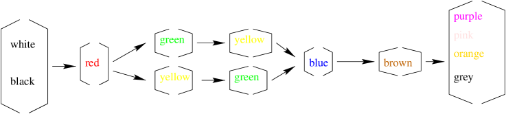
Figure 16: The Berlin-Kay Universal Colour Partial Ordering

CP4) Focal colours are more memorable and easier to recognize than any other colours, whether or not the subject speak a language having a name for the colour.
CP5) The structure of the colour space determined by multi-dimensional scaling of perceptual data is probably the same for all human communities and it is unrelated to the space yielded by naming data.
Again there is a culturally determined linguistic partial ordering (or hierarchy). On this occasion it determines the semantic content of individual words rather than syntax rules. Again there appears to be nothing known on how the skill develops in an individual, or any timing tests on the possession of a colour name strategy. The existence of two separate hierarchical partial orderings suggests that there is a general mechanism for there construction. Most members of a community seem to develop these culturally determined skills suggesting that the capacity to develop them is usually innate but their manifestation depends on environment.

References

-
[1]
Baldi,P. and BaumE.B.(1986)
Bounds on the Size of Ultrametric Structures.
Phys.Rev.Lett. 56, 1598-1600. -
[2]
Brekke,L. and Freund,P.G.O.(1993)
P-adelic numbers in Physics.
Math.Rev.94h:11115 Phys.Rep. 233, 1-66,
especially sections 10 and 13.4. -
[3]
Berlin,B and Kay,P.(1969)
Basic Colour Terms,
University of California Press. -
[4]
Bjorken,J.D. and Drell,S.D.(1965)
Relativistic Quantum Fields,
Math.Rev.66:5092
McGraw Hill, New York. p.378. -
[5]
Boettcher,S. and Paczuski,M.(1997)
Aging in a model of Self-Organized Criticality.
cond-mat/9603120 Phys.Rev.Lett. 79, 889. -
[6]
Chomsky, N.(1986a)
Knowledge of Language, Its Nature, Orgin and Use.
Praeger Publishers, New York. -
[7]
Chomsky, N.(1986b)
Barriers,
MIT Press, Cambridge, MA. -
[8]
Christiansen, Henning(2001)
CHR as Grammar Formalism.
http://arXiv.org/abs/cs.PL/0106059 -
[9]
Cowan, Nelson.(2001)
The Magical Number 4 in Short-term Memory:
A Reconsideration of Mental Storage Capacity.
Behavioral & Brain Sciences24 (1): XXX-XXX. -
[10]
Delon,F.(1984)
Espaces Ultramétriques.
Math.Rev.85i:03116 J. Symbolic Logic 49, 405. -
[11]
Guénoche,A.(1997)
Order distance associated with hierarchy.
Math.Rev.98d:62108 J.Classification 14, 101. -
[12]
Frazier,Lyn(1987)
Sentence Processing: A Tutorial Review.
Attention & PerformanceXII,p559-586
The Psychology of Reading, edited Max Coltheart. -
[13]
Haegeman, L.(1994)
Introduction to Government and Binding Theory,
First Edition (1991), Second Edition (1994), Blackwell, Oxford. -
[14]
Hammer,H.(1998)
Tree structure, Entropy, and the
Action Principle for Neighbourhood Topologies.
hep-th/9811118 -
[15]
Higgs,P.G.(1996)
Overlaps between RNA Secondary Structure.
Phys.Rev.Lett. 76, 704-707. -
[16]
Jackendoff,R.S(1977)
X̄ Syntax. A Study of Phrase Structure.
MIT Press, Cambridge, Mass. -
[17]
Jardine,N. and Sibson,R.(1971)
Mathematical Taxonomy,
John Wiley and Sons. -
[18]
Karwowski,W. and Mendes,R.V.(1994)
Hierarchical structures and asymmetric stochastic processes
on p-adics and adeles.
Math.Rev.95h:60166 J.Math.Phys. 35, 4637. -
[19]
Kayne,R.S.(1981)
Unambiguous Paths, Ch.5 in
Levels of Syntactic Representation,
Edited by Robert May and Jan Koster,
Foris Publications, Dordrecht. -
[20]
Keenan,E.L. and Comrie,B.(1977)
Noun Phrase Accessibility and Universal Grammar.
Linguistic Inquiry 8, 63-99. -
[21]
Lockward,D.G.(1972)
Introduction to Stratification Grammar.
Harcourt Brace Jovanovich Inc.,New York. -
[22]
McCloskey,J.(1988)
Syntatic Theory,
p.18 in Linguistics: The Cambridge Survey,
Cambridge University Press, Cambridge. -
[23]
Miller,G.A.(1956)
The magical number seven, plus or minus two:
some limits on our capacity to process information.
http://cogprints.soton.ac.uk/abs/psy/199807022
Psy.Rev. 63,81-97. -
[24]
Ogielchi,A.T. and Stein,D.L.(1985)
Dynamics on Ultrametric Spaces.
Math.Rev.86j:82051
Phys.Rev.Lett. 55, 1634-1637. -
[25]
Parga,N. and Virasoro,M.A.(1986)
The Ultrametric Organization of Neural Net Memories.
J.de Physique 47, 1857. -
[26]
Perlman,E.M. and Schwarz,M.(1992)
The Directed Polymer Problem.
Europhys.Lett. 17, 227. -
[27]
Prince,A. and Smolensky,P.(1997)
Optimality: From Neural Networks to Universal Grammar.
Science 275,1604. -
[28]
Rammal,R., Toulouse,G. and Virasoro,M.A.(1986)
Ultrametricity for Physicists.
Math.Rev.87k:82105 Rev.Mod.Phys. 58, 765-788. -
[29]
Rissanen,Jorma(1983)
A universal prior for integers and estimation
by minimum description lenght.
Math.Rev.85i:62002
Annals of Statistics 11,416-431. -
[30]
Roberts.Mark D.
P-model Alternative to the T-model.
http://arXiv.org/abs/cs.CL/9811018 -
[31]
Roberts.Mark D.
Name Strategy: Its Existence and Implications.
http://arXiv.org/abs/cs.CL/9812004 -
[32]
Rutten,J.,J.,M.,M.,(1996)
Elements of Generalized Ultrametric Domain Theory.
Theor.Comp.Sci. 170, 349. -
[33]
Shepard,R.N. and Arabie,P.(1979)
Additive Clustering: Representative of Similarities
as Combinations of Discrete Overlapping Properties.
Psychological Review 86, 87-123, especially page 90. -
[34]
Sneath,P.H. and Sokal,R.R.(1973)
The Principles and Practice of Numerical Classification.
W.H.Freeman and Company, San Francisco. -
[35]
Sorton, George(1947)
Introduction to the History of Science, Vol.III, page552
The Williams and Wilkins Company, Baltimore. -
[36]
Vlad, M.O.(1994)
Fractal time, ultrametric topology and fast relation.
Math.Rev.95a:82061
Phys.Lett. A189, 299-303. -
[37]
Weissman,M.,B.(1993)
What is Spin Glass.
Rev.Mod.Phys. 65, 829. -
[38]
Young,M.R. and DeSarbo,W.S.(1995)
A Parametric procedure for Ultrametric tree estimation from conditional rank order proximity data.
Psychometrika 60,47. -
[39]
Zadrozny,Wlodek (2000)
Minimum Description Lenght and Compositionality.
http://arXiv.org/abs/cs.CL/0001002
H.Blunt and R.Muskens (Eds) Computing Meaning Vol. 1, Kluwer 1999, pp113-128.