A Linear Shift Invariant Multiscale Transform

Abstract

This paper presents a multiscale decomposition algorithm. Unlike standard wavelet transforms, the proposed operator is both linear and shift invariant. The central idea is to obtain shift invariance by averaging the aligned wavelet transform projections over all circular shifts of the signal. It is shown how the same transform can be obtained by a linear filter bank.

1 Introduction

Images typically contain information at many different scales. For applications such as image retrieval, it is therefore highly desirable to decompose images orthogonally into subbands. This can be done using wavelet transforms [8].

However, the standard wavelet transforms are shift variant, i.e. a small shift of the signal can change the wavelet transform coefficients quite dramatically. As a result, those coefficients cannot be used for image retrieval when shifts of the original image can occur.

Several schemes have been proposed recently to introduce shift invariance into the framework of wavelet transforms. An early approach was to look at the extrema only of the wavelet transform modulus [9]. Several authors suggested the introduction of a cost function in order to come up with a unique best basis [2, 4, 7]. A cost function that figures prominently is the entropy cost function used in [3]. Note that the best basis of a structure might change if it is embedded into a larger structure. Filter oriented approaches have been introduced in [5] and [14].

Most approaches cited above use a notion of shift invariance, called $\mu-translation-invariance$ in [7] and near shift invariance in [5], that is different from the standard usage. They take shift invariance to imply that the wavelet transform coefficients do not change at all if the signal is shifted. However, they extract the different delays of translated signals. By contrast, we stick with the standard definition of shift invariance which means that the operator output is shifted proportionally to the shift of the input signal. In [11], it is shown that shift invariance (referred to as shiftability in that paper) cannot be achieved by a critically sampling transform like the wavelet transform because of aliasing.

In this paper, we propose a decomposition algorithm called the Averaged Wavelet Transform (AWT) that incorporates shift invariance in the standard sense. It delivers a unique representation of a signal without requiring a cost function.

Systems using wavelets for the purpose of classification and retrieval have been described in [6, 10, 13].

2 The Averaged Wavelet Transform

In one dimension, we define the AWT to be a mapping from a discrete signal $SIG$ of length $n$ to $k+1$ vectors of the same length $n$, where $k$ is the number of decomposition levels which is logarithmic in $n$. That is,

$$AWT:R^{n}\rightarrow R^{n}\times R^{n}\times\dots\ \ (\mathrm{k+1\ \ times})$$

The key idea for obtaining a shift invariant signal decomposition is to average the projections of the signal onto the wavelet subspace at each scale over all circular shifts of the input signal. We call the result the scale spectra of the signal. Note that those projections are sometimes also referred to as detail vectors, or reconstructed details, or just details.

More precisely, let $WT$ be a discrete wavelet transform, let $CS_{i}$ be the circular right shift operator (performing $i$ right shifts), with $CS_{i}^{-1}$ analogously being the circular left shift operator, and let $REC_{s}$ be the reconstruction operator that projects the signal onto the wavelet subspace at scale $s,s=0..k$, with the special case $s_{0}$ being the DC component.

Then the AWT at scale $s$ is

$$AWT_{s}=\frac{1}{n}\sum_{i=0}^{n-1}CS_{i}^{-1}(REC_{s}(WT(CS_{i}(SIG))))$$

The left shift operator $CS_{i}^{-1}$ is applied to compensate for the shifting of the signal, i.e. we average over the projections that are aligned to the position of the signal before shifting. The complete AWT is the set of all $AWT_{s},s=0..k$.

The shift invariance of this approach follows directly from the nature of the averaging process: if the input signal is shifted, the AWT is still computed over the same set of $n$ circularly shifted signals. Also, as an inherent property of the averaging operation, the AWT is linear. Like the standard WT, the AWT decomposes a signal into a DC component and scale spectra of zero mean, with some frequency overlap between the scale spectra. Adding a constant to all signal values only changes the DC component, but not the scale spectra.

The AWT is information preserving. The original signal can be easily reconstructed by just adding up the scale spectra, i.e.

$$SIG=\sum_{s=0}^{k}AWT_{s}$$

In this sense, the summation is the inverse transform of the AWT. Note that the AWT is highly redundant. It increases the space requirement by a factor of $k+1$. However, for most applications, the scale spectra will serve only as an intermediate representation. Typically, it suffices to keep only a few features which are derived from the scale spectra.

The generalization from 1-d to 2-d is conceptually straightforward, albeit computationally expensive. The circular shifting has to be done over all shifts along the two axes, and the 1-d wavelet transform is replaced by a 2-d WT. Fortunately, an efficient algorithm to compute the wavelet coefficients of all $n$ circular shifts of a vector of length $n$ in $O(n\ \mathrm{lg}\>n)$ time, rather than the $O(n^{2})$ time of the naive approach, is given in [1], based on the observation that the shift operation is sparse. [7] describes the extension of Beylkin’s algorithm to 2-d.

3 Emulation of the AWT by a Filter Bank

As pointed out above, the AWT is a shift invariant linear transform. As such, the AWT is well defined by a single impulse response for each scale spectrum. This means that we have to compute the underlying set of AWT filters only once, and then the AWT can be computed simply and efficiently by convolution of the signal with those AWT filters.

The filter bank that emulates an AWT depends on the type of wavelet chosen for the wavelet transform and on the size of the signal – each signal size has its own corresponding AWT filter bank. The AWT filters are symmetric and therefore linear phase. By construction, their length is bounded by the signal length, so they are FIR filters.

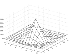
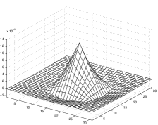
Figure 1: AWT filters (Haar), 1-d and 2-d, consecutive scales, signal length is a power of two

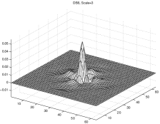
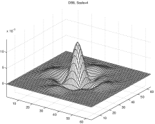
Figure 2: AWT filters (Daub₈), 1-d and 2-d, consecutive scales, signal length is a power of two

The simplest AWT filter bank is obtained for the Haar wavelet with a signal length that is a power of two. They turn out to be dilations of the hat function, shown in fig. 1 for the first three 1-d scales and for two scales in the 2-d case. In the 1-d case, the filter coefficients are (-0.25 0.5 -0.25), (-0.0625 -0.125 0.0625 0.25 0.0625 -0.125 -0.0625) for scale one and two, respectively. The AWT filters $y^{(i)}(x)$ at scale $i$ are easily computed from the filter at scale $1$ by the formula $y^{(i)}(x)=2^{-(i-1)}y^{(1)}(2^{-(i-1)}x)$ which nicely reflects their wavelet transform origin. Although these AWT filters are the solution of a dilation equation, they are not wavelets [12]: they are orthogonal to only some of their translates and dilations. This comes as no surprise, since it was shown in [11] that shiftability can only be achieved by relaxing the orthogonality property of the wavelet transform. Clearly, the AWT is not a pure wavelet transform, and it doesn’t provide for a multiresolution [8]. Note also that the formula for AWT filters for Haar wavelets does not generalize to signal sizes that are not a power of two or to other types of wavelets. Fig. 2 shows some of the AWT filters derived from Daubechies-8 wavelets.

4 Experiments

Figure 3 demonstrates the decomposition of a 1-d signal (it happens to be a cross section of the image in fig. 5) by the AWT, and the shift invariance of the latter: all scale spectra of the circularly shifted signal are also circularly shifted by the same amount. We have chosen Haar wavelets here, but the AWT works for any wavelet. While a standard Haar wavelet transform results in projections that are step functions, the AWT gives a much smoother decomposition.

Figure 3: (top) AWT of a signal,  (bottom) AWT of the same signal, but circularly right shifted by 20 units.

Figure 4: (top) AWT of a substructure of the signal in fig. 3,   (bottom) AWT of the shifted substructure.

Figure 4 demonstrates the usefulness of the AWT for the retrieval of image substructures at various scales. The signal now consists of a small substructure of the signal in fig. 3, with the rest of the signal being set to zero. Again, the AWT decomposition of this signal is given at the top, and the AWT of the same substructure, circularly right shifted, at the bottom.

It can be observed that the AWT of the substructure matches the corresponding part of the AWT of the full signal to a large degree, depending on the scale. At small scales, the filter support is small and therefore localized. By contrast, at large scales, the area of support is large, which means that the filter response to a small substructure is influenced to a large degree by the surrounding signal, i.e. adjacent structures. It is also evident that the substructure cut-off may introduce an edge artifact.

Figure 5 gives an example of applying the 2-d AWT, based on the Haar wavelet, to an image. The six scale spectra plus the DC component add up to the original signal.

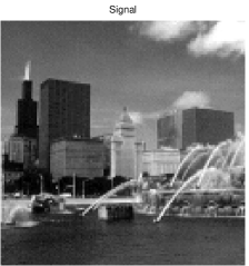
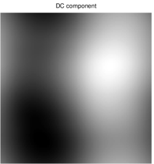
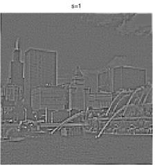
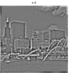
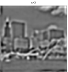
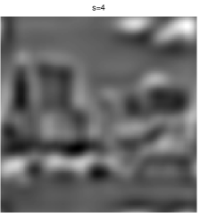
Figure 5: 2-d AWT (Haar, 128$\times$128). Original Image, DC component, six dyadic scales.

Acknowledgements

I would like to thank B. Woodham for his valuable critique.

References

- [1] G. Beylkin, “On the Representation of Operators in Bases of Compactly Supported Wavelets”, SIAM J. Numerical Analysis, Dec.1992.
- [2] I. Cohen, S. Raz, D. Malah, “Shift Invariant Wavelet Packet Bases”, ICASSP-95, Detroit 1995.
- [3] R. Coifman, M. Wickerhauser, “Entropy-Based Algorithms for Best Basis Selection”, IEEE Trans. Information Theory, Vol.38, No.2, pp.713-718, Mar.1992.
- [4] S. Del Marco, P. Heller, J. Weiss, “An M-Band, 2-Dimensional Translation-Invariant Wavelet Transform and Applications”, ICASSP-95, Detroit 1995.
- [5] Y. Hui, C. Kok, T. Nguyen, “Shift-Invariant Filter Banks: Theory, Design, and Applications” submitted to IEEE Trans. Signal Processing.
- [6] C. Jacobs, A. Finkelstein, D. Salesin, “Fast Multiresolution Image Querying”, Computer Graphics Proc., pp.277-286, 1995.
- [7] J. Liang, T. Parks, “A two-dimensional Translation Invariant Wavelet Representation and its Applications”, ICIP-94, Austin 1994.
- [8] S. Mallat, “A Theory for Multiresolution Signal Decomposition: The Wavelet Representation”, IEEE Trans. PAMI, Vol.11, No.7, pp.674-693, July 1989.
- [9] S. Mallat, W. Hwang, “Singularity Detection and Processing with Wavelets”, IEEE Trans. Information Theory, Vol.38, No.2, pp.617-643, Mar.1992.
- [10] M. Oren, C. Papageorgiou, P. Sinha, E. Osuna, T. Poggio, “Pedestrian Detection Using Wavelet Templates”, CVPR ’97, Puerto Rico 1997.
- [11] E. Simoncelli, W. Freeman, E. Adelson, D. Heeger, “Shiftable Multiscale Transforms”, IEEE Trans. Information Theory, Vol.38, No.2, pp.587-607, Mar.1992.
- [12] G. Strang, “Wavelets and Dilation Equations: A Brief Introduction”, SIAM Review, Vol.31, No.4, pp.613-627, Dec.1989.
- [13] B. Telfer et al., “Adaptive wavelet classification of acoustic backscatter and imagery”, Optical Engineering, Vol.33, No.7, pp.2192-2203, July 1994.
- [14] J. Zhou, X. Fang, B. Ghosh, “Image Segmentation based on Multiresolution Filtering”, ICIP-94, Austin 1994.